

Compact Muon Solenoid
LHC, CERN
| CMS-PAS-TOP-23-004 | ||
| Inclusive and differential measurement of top quark cross sections in association with a Z boson | ||
| CMS Collaboration | ||
| 27 March 2024 | ||
| Abstract: A measurement is presented of the inclusive and differential cross sections for top quark production in association with a Z boson, in pairs ($ \mathrm{t\bar{t}Z} $) or with a single top quark ($ \mathrm{tZq} $ and $ \mathrm{tWZ} $). The data were recorded in pp collisions at a center-of-mass energy of 13 TeV, corresponding to an integrated luminosity of 138 fb$ ^{-1} $. Events with exactly three leptons, electrons or muons, are selected. A deep neural network is trained to separate the signal processes and the backgrounds. The $ \mathrm{t\bar{t}Z} $ and $ \mathrm{tWZ} $ processes are measured together due to their similar experimental signature and significant interference beyond leading order. A combined profile likelihood approach is used to unfold the differential cross sections, to account for systematic uncertainties, and to determine the correlations between the two signal categories in one global fit. The inclusive cross sections for a dilepton invariant mass within 70 and 110 GeV are measured to be 1.14 $ \pm $ 0.07 pb for the sum of $ \mathrm{t\bar{t}Z} $ and $ \mathrm{tWZ} $, and 0.81 $ \pm $ 0.10 pb for $ \mathrm{tZq} $. While good agreement of the data with the standard model prediction is found for the $ \mathrm{tZq} $ process, the measured inclusive cross section for $ \mathrm{t\bar{t}Z}+\mathrm{tWZ} $ has a ratio to the central value of the prediction of 1.17 $ \pm $ 0.07. | ||
| Links: CDS record (PDF) ; Physics Briefing ; CADI line (restricted) ; | ||
| Figures | |

png pdf |
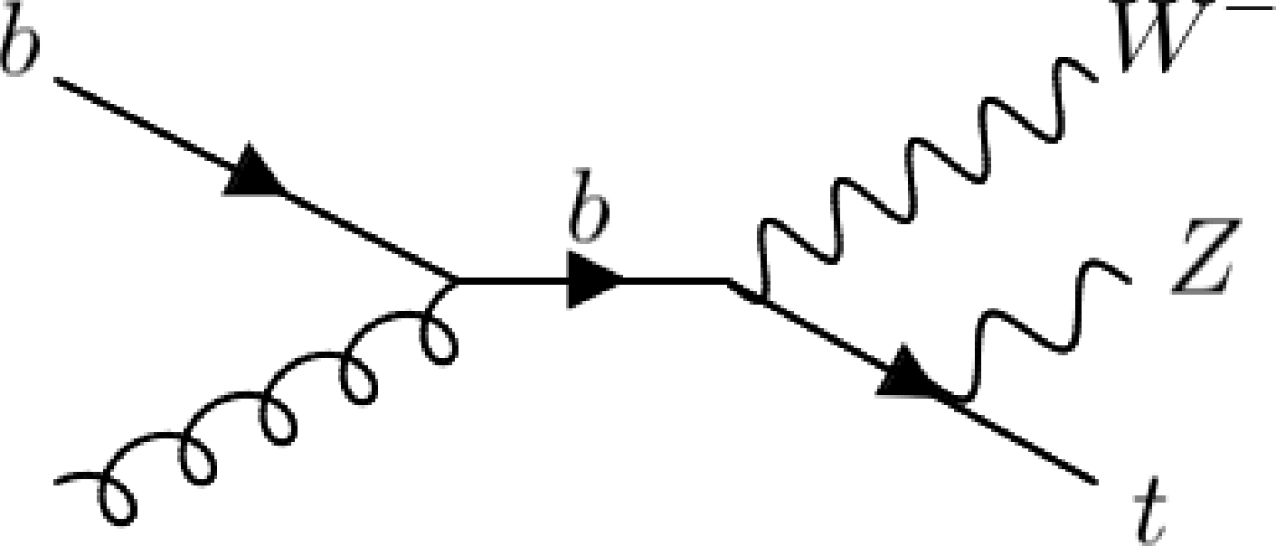
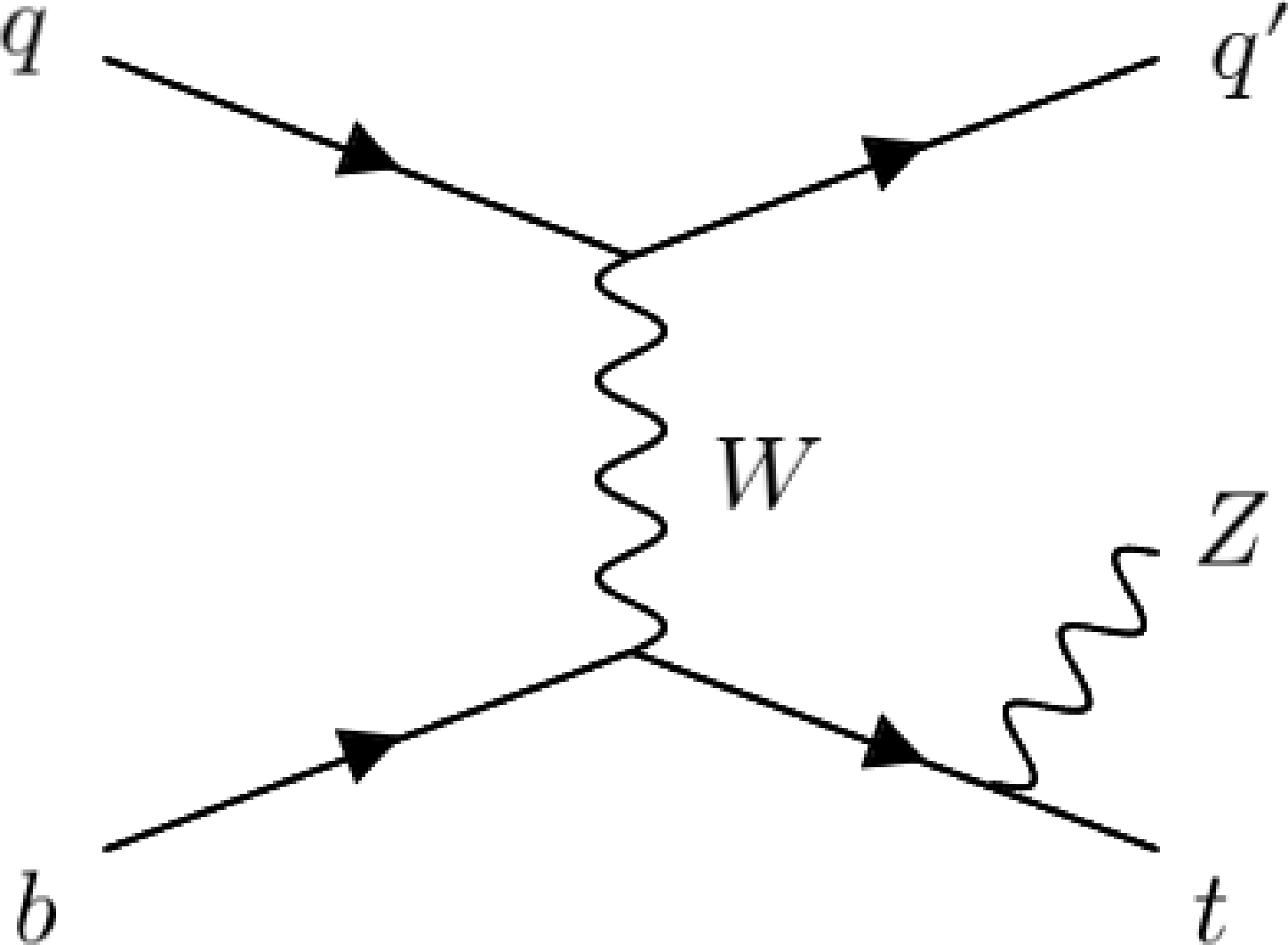
Figure 1:
Leading order diagrams for the $ {\mathrm{t}\overline{\mathrm{t}}} \mathrm{Z} $ (left), $ \mathrm{t}\mathrm{W}\mathrm{Z} $ (middle), and $ \mathrm{t}\mathrm{Z}\mathrm{q} $ (right) processes. |

png pdf |
Figure 1-a:
Leading order diagrams for the $ {\mathrm{t}\overline{\mathrm{t}}} \mathrm{Z} $ (left), $ \mathrm{t}\mathrm{W}\mathrm{Z} $ (middle), and $ \mathrm{t}\mathrm{Z}\mathrm{q} $ (right) processes. |
png pdf |
Figure 1-b:
Leading order diagrams for the $ {\mathrm{t}\overline{\mathrm{t}}} \mathrm{Z} $ (left), $ \mathrm{t}\mathrm{W}\mathrm{Z} $ (middle), and $ \mathrm{t}\mathrm{Z}\mathrm{q} $ (right) processes. |
png pdf |
Figure 1-c:
Leading order diagrams for the $ {\mathrm{t}\overline{\mathrm{t}}} \mathrm{Z} $ (left), $ \mathrm{t}\mathrm{W}\mathrm{Z} $ (middle), and $ \mathrm{t}\mathrm{Z}\mathrm{q} $ (right) processes. |
png pdf |
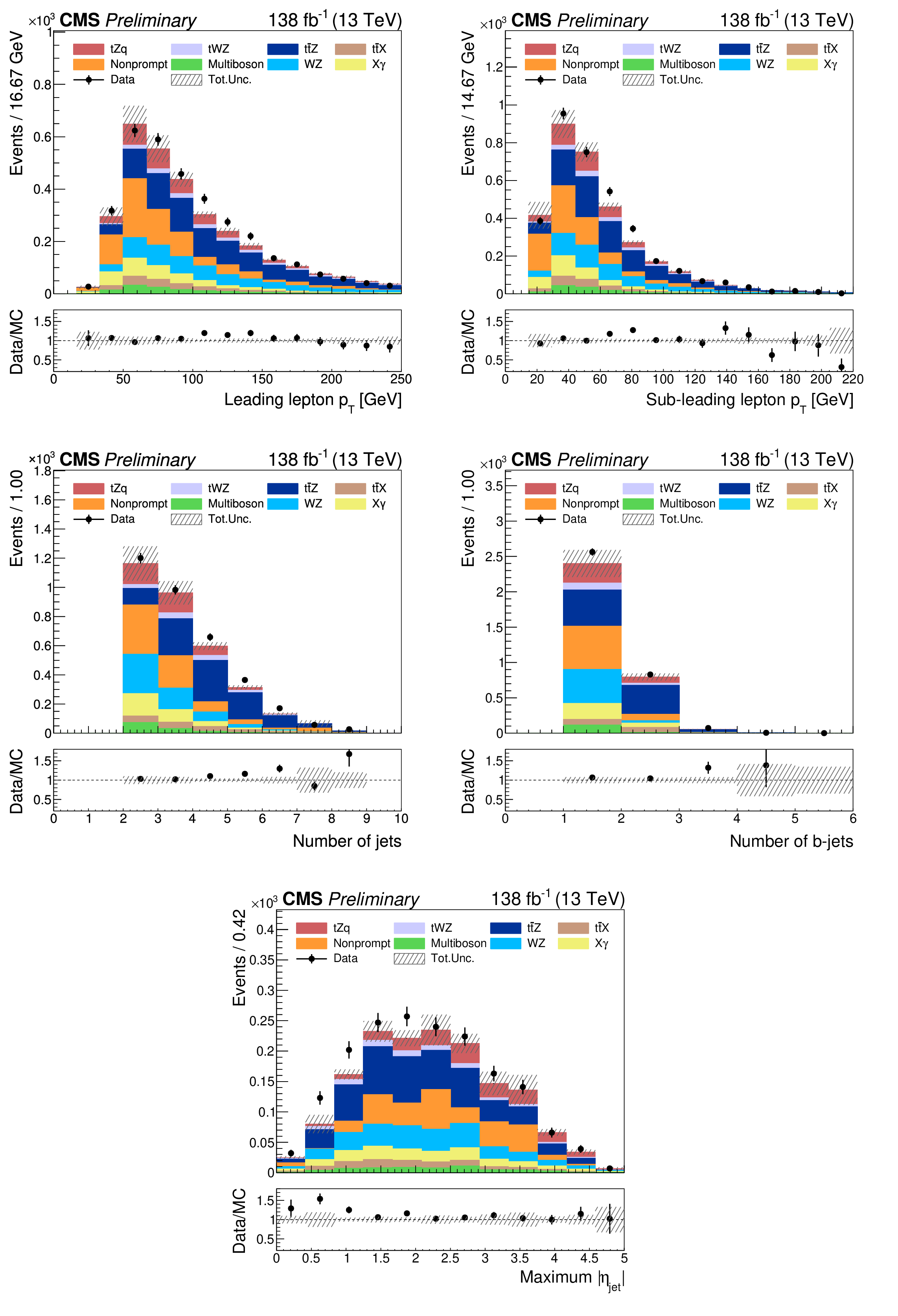
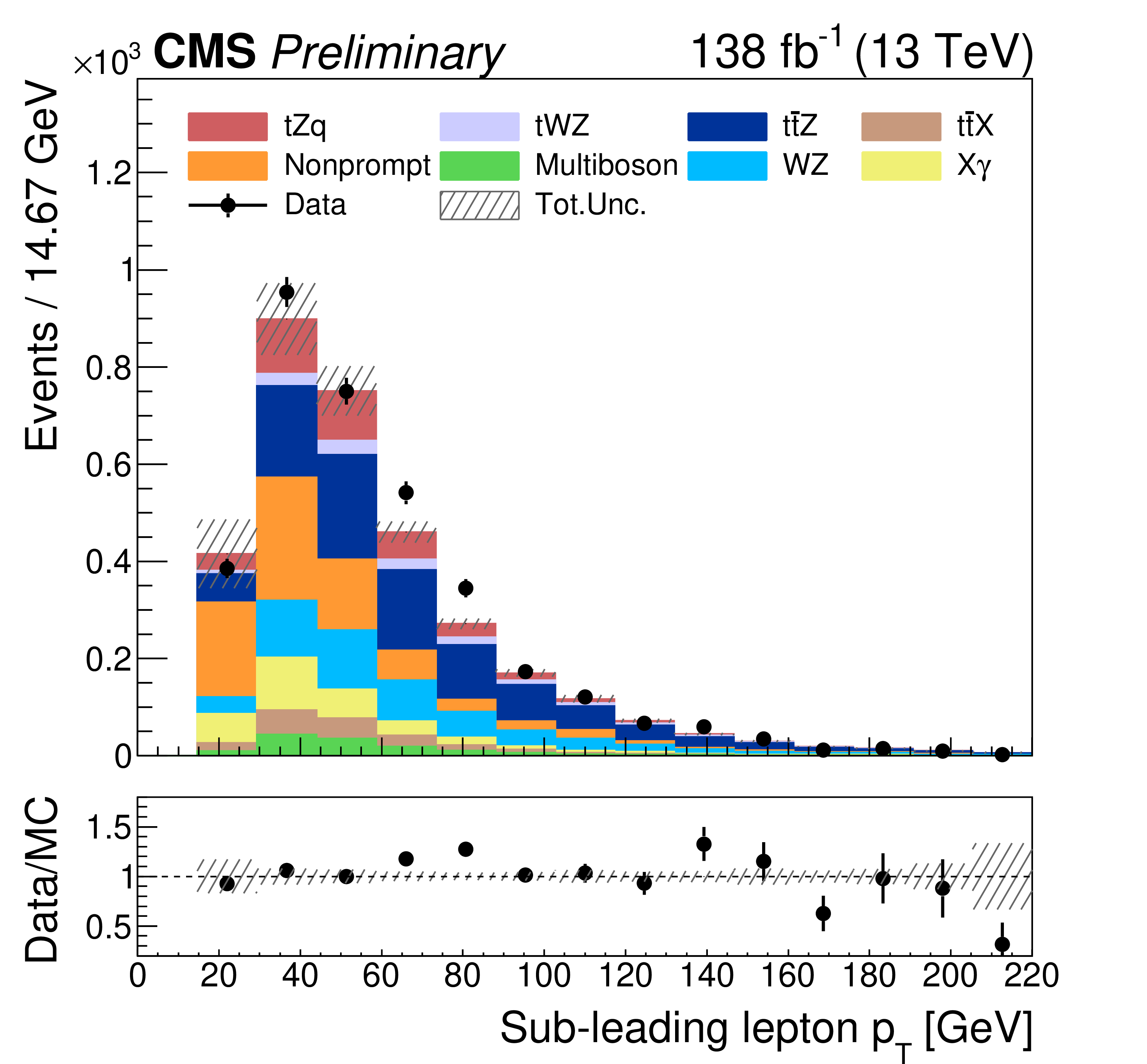
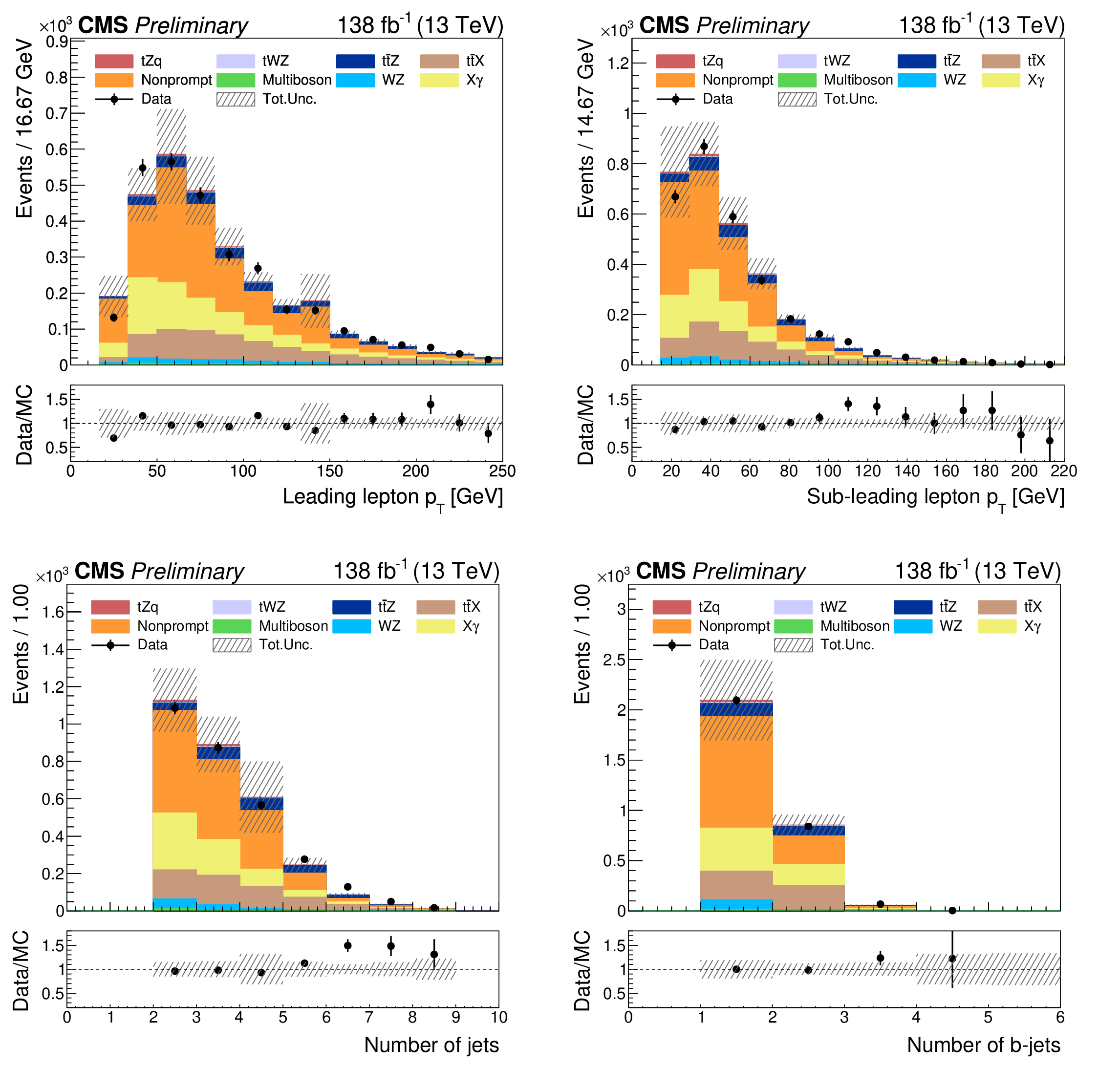
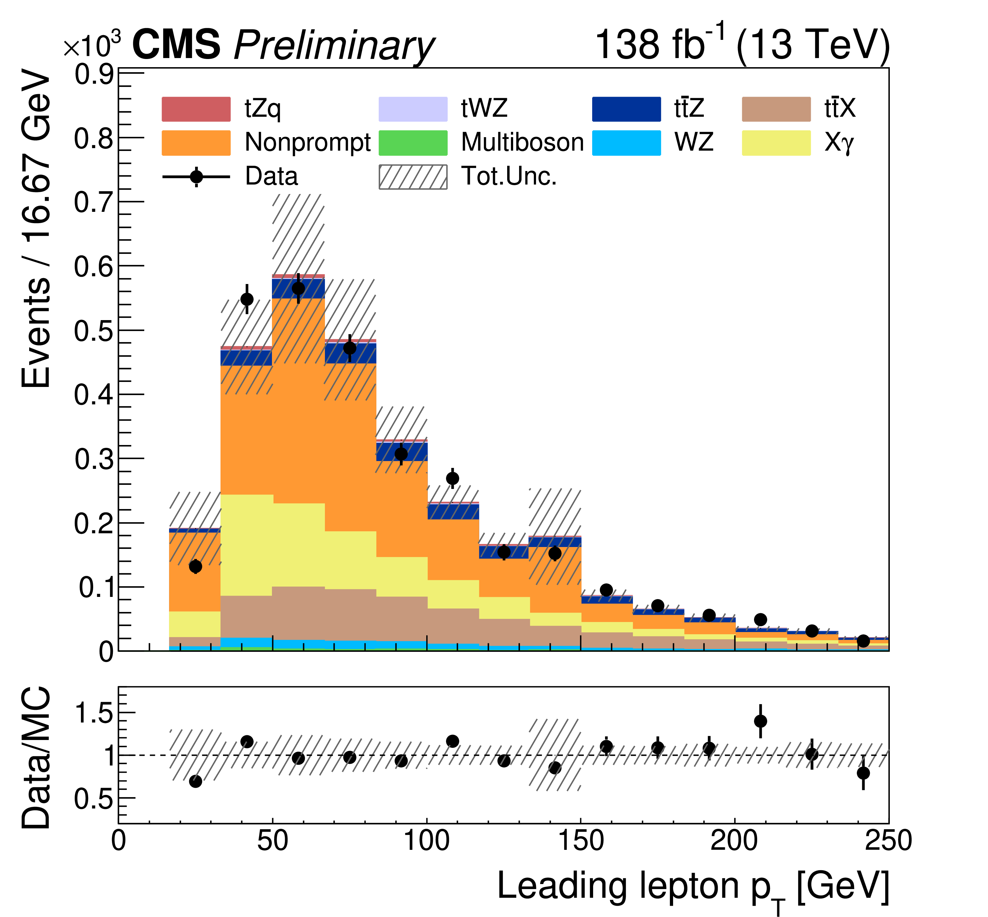
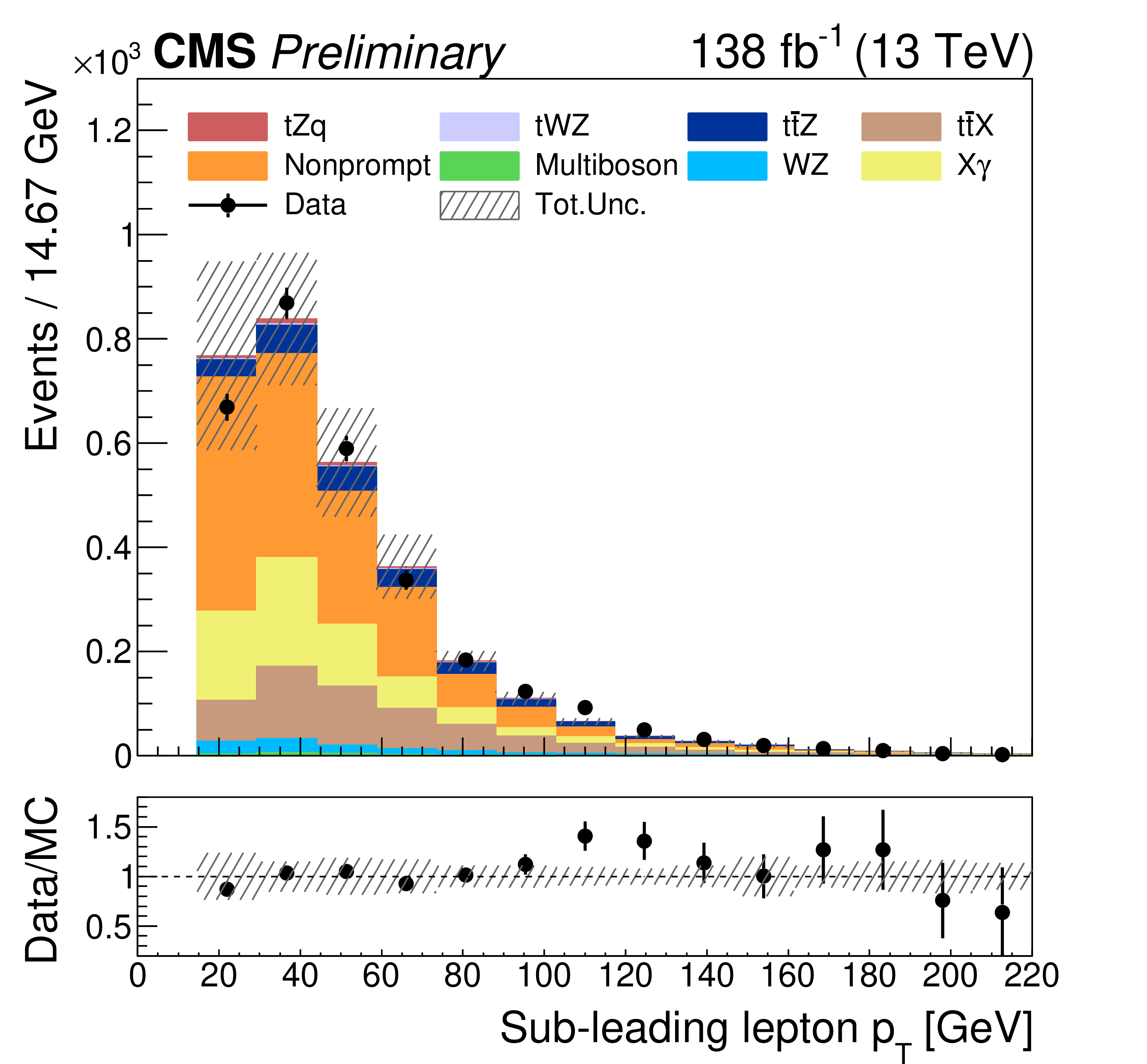
Figure 2:
Distributions after final event selection for: the $ p_{\mathrm{T}} $ of the lepton with the highest (upper left) and second highest (upper right) transverse momentum, the number of jets (middle left), the number of b jets (middle right), and the $ |\eta| $ of the jet with the highest pseudorapidity. The data and their statistical uncertainties are indicated by bullets and error bars. The hatched area indicates the systematic uncertainty in the expectation, including the statistical uncertainty of the MC samples. In the legend, "$ {\mathrm{t}\overline{\mathrm{t}}} $X" refers to backgrounds involving the associated production of top quarks with bosons (e.g., $ {\mathrm{t}\overline{\mathrm{t}}} \mathrm{W} $, $ {\mathrm{t}\overline{\mathrm{t}}} \mathrm{H} $), and "X$ \gamma $" denotes the associated production of bosons and photons. |
png pdf |
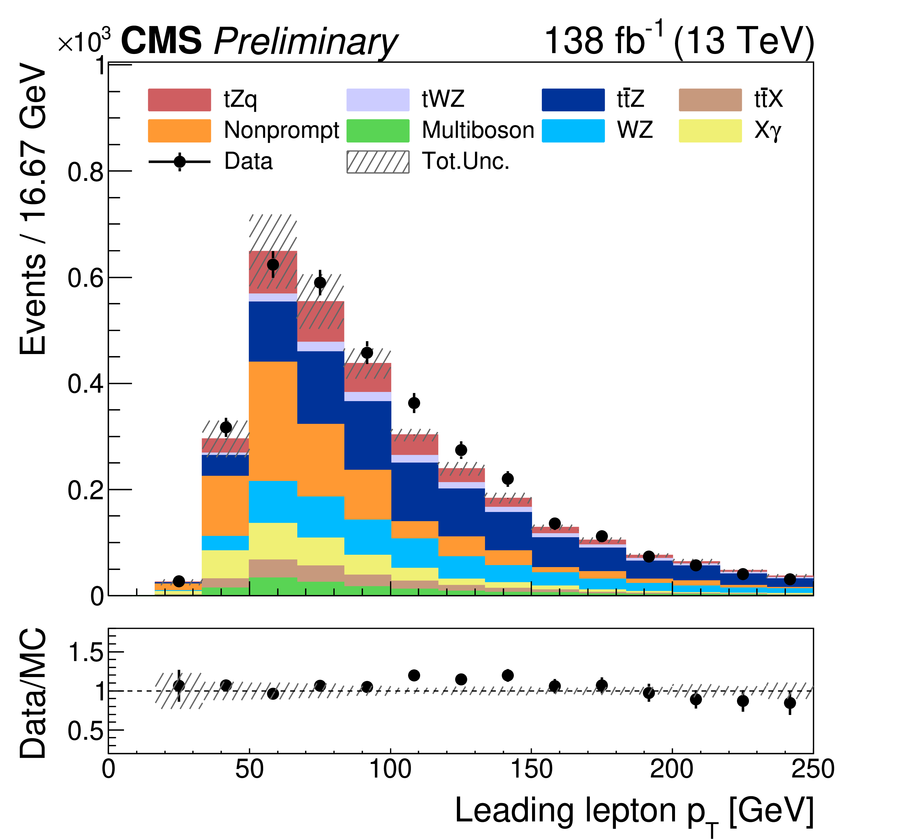
Figure 2-a:
Distributions after final event selection for: the $ p_{\mathrm{T}} $ of the lepton with the highest (upper left) and second highest (upper right) transverse momentum, the number of jets (middle left), the number of b jets (middle right), and the $ |\eta| $ of the jet with the highest pseudorapidity. The data and their statistical uncertainties are indicated by bullets and error bars. The hatched area indicates the systematic uncertainty in the expectation, including the statistical uncertainty of the MC samples. In the legend, "$ {\mathrm{t}\overline{\mathrm{t}}} $X" refers to backgrounds involving the associated production of top quarks with bosons (e.g., $ {\mathrm{t}\overline{\mathrm{t}}} \mathrm{W} $, $ {\mathrm{t}\overline{\mathrm{t}}} \mathrm{H} $), and "X$ \gamma $" denotes the associated production of bosons and photons. |
png pdf |
Figure 2-b:
Distributions after final event selection for: the $ p_{\mathrm{T}} $ of the lepton with the highest (upper left) and second highest (upper right) transverse momentum, the number of jets (middle left), the number of b jets (middle right), and the $ |\eta| $ of the jet with the highest pseudorapidity. The data and their statistical uncertainties are indicated by bullets and error bars. The hatched area indicates the systematic uncertainty in the expectation, including the statistical uncertainty of the MC samples. In the legend, "$ {\mathrm{t}\overline{\mathrm{t}}} $X" refers to backgrounds involving the associated production of top quarks with bosons (e.g., $ {\mathrm{t}\overline{\mathrm{t}}} \mathrm{W} $, $ {\mathrm{t}\overline{\mathrm{t}}} \mathrm{H} $), and "X$ \gamma $" denotes the associated production of bosons and photons. |

png pdf |
Figure 2-c:
Distributions after final event selection for: the $ p_{\mathrm{T}} $ of the lepton with the highest (upper left) and second highest (upper right) transverse momentum, the number of jets (middle left), the number of b jets (middle right), and the $ |\eta| $ of the jet with the highest pseudorapidity. The data and their statistical uncertainties are indicated by bullets and error bars. The hatched area indicates the systematic uncertainty in the expectation, including the statistical uncertainty of the MC samples. In the legend, "$ {\mathrm{t}\overline{\mathrm{t}}} $X" refers to backgrounds involving the associated production of top quarks with bosons (e.g., $ {\mathrm{t}\overline{\mathrm{t}}} \mathrm{W} $, $ {\mathrm{t}\overline{\mathrm{t}}} \mathrm{H} $), and "X$ \gamma $" denotes the associated production of bosons and photons. |

png pdf |
Figure 2-d:
Distributions after final event selection for: the $ p_{\mathrm{T}} $ of the lepton with the highest (upper left) and second highest (upper right) transverse momentum, the number of jets (middle left), the number of b jets (middle right), and the $ |\eta| $ of the jet with the highest pseudorapidity. The data and their statistical uncertainties are indicated by bullets and error bars. The hatched area indicates the systematic uncertainty in the expectation, including the statistical uncertainty of the MC samples. In the legend, "$ {\mathrm{t}\overline{\mathrm{t}}} $X" refers to backgrounds involving the associated production of top quarks with bosons (e.g., $ {\mathrm{t}\overline{\mathrm{t}}} \mathrm{W} $, $ {\mathrm{t}\overline{\mathrm{t}}} \mathrm{H} $), and "X$ \gamma $" denotes the associated production of bosons and photons. |

png pdf |
Figure 2-e:
Distributions after final event selection for: the $ p_{\mathrm{T}} $ of the lepton with the highest (upper left) and second highest (upper right) transverse momentum, the number of jets (middle left), the number of b jets (middle right), and the $ |\eta| $ of the jet with the highest pseudorapidity. The data and their statistical uncertainties are indicated by bullets and error bars. The hatched area indicates the systematic uncertainty in the expectation, including the statistical uncertainty of the MC samples. In the legend, "$ {\mathrm{t}\overline{\mathrm{t}}} $X" refers to backgrounds involving the associated production of top quarks with bosons (e.g., $ {\mathrm{t}\overline{\mathrm{t}}} \mathrm{W} $, $ {\mathrm{t}\overline{\mathrm{t}}} \mathrm{H} $), and "X$ \gamma $" denotes the associated production of bosons and photons. |

png pdf |
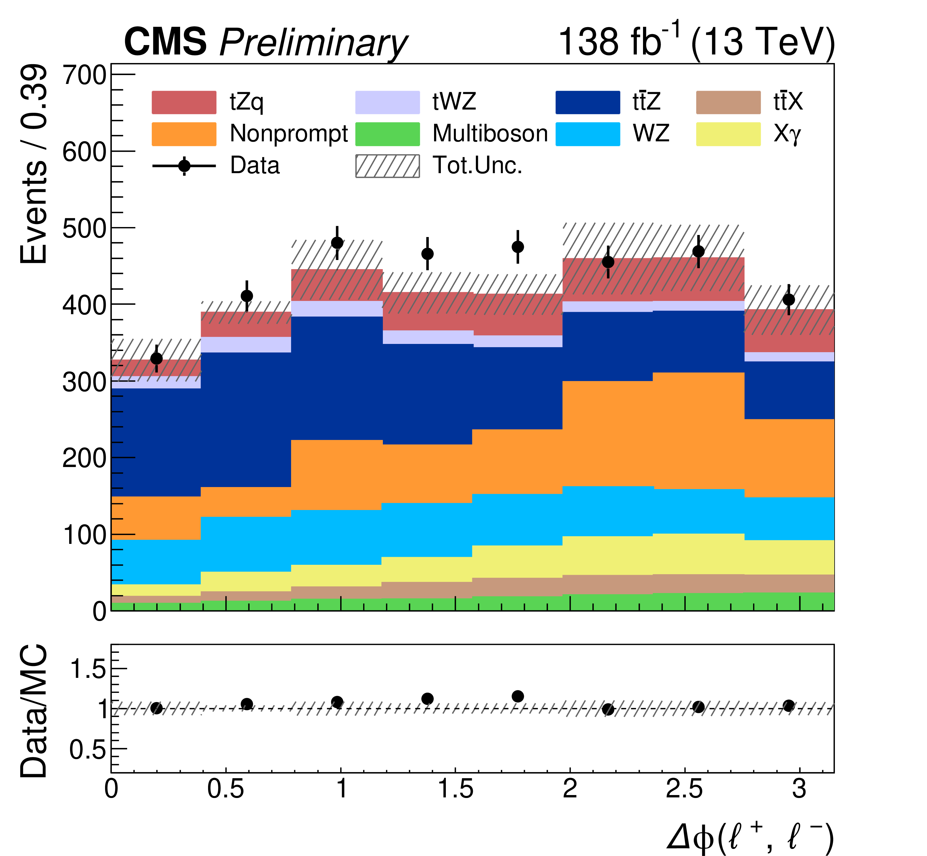
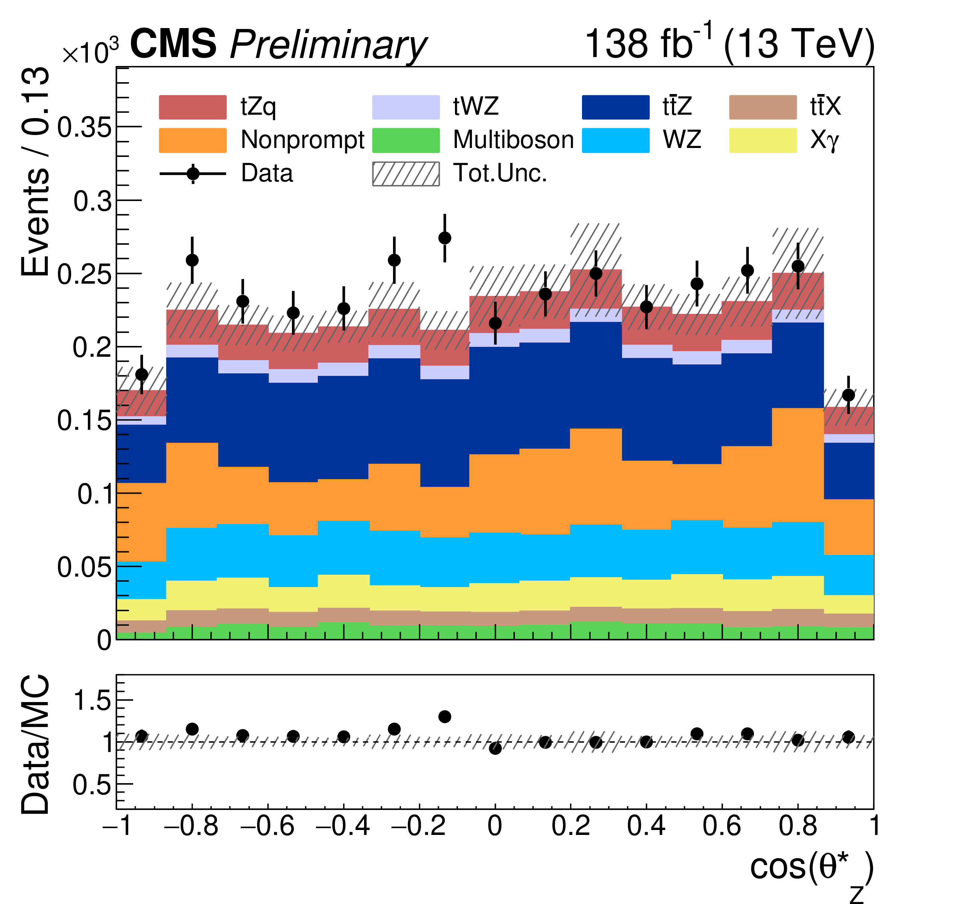
Figure 3:
Distributions after final event selection for: the $ p_{\mathrm{T}} $ of the reconstructed Z boson (upper left), the $ p_{\mathrm{T}} $ of the lepton arising from the W boson $ p_{\mathrm{T}}(\ell_\mathrm{W}) $ (upper right), $ \Delta R(\mathrm{Z}, \ell_\mathrm{W}) $ (middle left), $ \Delta \phi(\ell^{+}, \ell^{-}) $ (middle right), and the cosine of the polar angle between the Z boson and its negatively charged decay lepton, boosted into the Z boson rest frame (lower). Further details are described in the caption of Fig. 2. |

png pdf |
Figure 3-a:
Distributions after final event selection for: the $ p_{\mathrm{T}} $ of the reconstructed Z boson (upper left), the $ p_{\mathrm{T}} $ of the lepton arising from the W boson $ p_{\mathrm{T}}(\ell_\mathrm{W}) $ (upper right), $ \Delta R(\mathrm{Z}, \ell_\mathrm{W}) $ (middle left), $ \Delta \phi(\ell^{+}, \ell^{-}) $ (middle right), and the cosine of the polar angle between the Z boson and its negatively charged decay lepton, boosted into the Z boson rest frame (lower). Further details are described in the caption of Fig. 2. |

png pdf |
Figure 3-b:
Distributions after final event selection for: the $ p_{\mathrm{T}} $ of the reconstructed Z boson (upper left), the $ p_{\mathrm{T}} $ of the lepton arising from the W boson $ p_{\mathrm{T}}(\ell_\mathrm{W}) $ (upper right), $ \Delta R(\mathrm{Z}, \ell_\mathrm{W}) $ (middle left), $ \Delta \phi(\ell^{+}, \ell^{-}) $ (middle right), and the cosine of the polar angle between the Z boson and its negatively charged decay lepton, boosted into the Z boson rest frame (lower). Further details are described in the caption of Fig. 2. |

png pdf |
Figure 3-c:
Distributions after final event selection for: the $ p_{\mathrm{T}} $ of the reconstructed Z boson (upper left), the $ p_{\mathrm{T}} $ of the lepton arising from the W boson $ p_{\mathrm{T}}(\ell_\mathrm{W}) $ (upper right), $ \Delta R(\mathrm{Z}, \ell_\mathrm{W}) $ (middle left), $ \Delta \phi(\ell^{+}, \ell^{-}) $ (middle right), and the cosine of the polar angle between the Z boson and its negatively charged decay lepton, boosted into the Z boson rest frame (lower). Further details are described in the caption of Fig. 2. |
png pdf |
Figure 3-d:
Distributions after final event selection for: the $ p_{\mathrm{T}} $ of the reconstructed Z boson (upper left), the $ p_{\mathrm{T}} $ of the lepton arising from the W boson $ p_{\mathrm{T}}(\ell_\mathrm{W}) $ (upper right), $ \Delta R(\mathrm{Z}, \ell_\mathrm{W}) $ (middle left), $ \Delta \phi(\ell^{+}, \ell^{-}) $ (middle right), and the cosine of the polar angle between the Z boson and its negatively charged decay lepton, boosted into the Z boson rest frame (lower). Further details are described in the caption of Fig. 2. |
png pdf |
Figure 3-e:
Distributions after final event selection for: the $ p_{\mathrm{T}} $ of the reconstructed Z boson (upper left), the $ p_{\mathrm{T}} $ of the lepton arising from the W boson $ p_{\mathrm{T}}(\ell_\mathrm{W}) $ (upper right), $ \Delta R(\mathrm{Z}, \ell_\mathrm{W}) $ (middle left), $ \Delta \phi(\ell^{+}, \ell^{-}) $ (middle right), and the cosine of the polar angle between the Z boson and its negatively charged decay lepton, boosted into the Z boson rest frame (lower). Further details are described in the caption of Fig. 2. |
png pdf |
Figure 4:
Distributions for events selected in the region with $ |m(\ell^{+}\ell^{-}) - m(\mathrm{Z})| > $ 20 GeV for: the $ p_{\mathrm{T}} $ of the lepton with the highest (upper left) and second highest (upper right) transverse momentum, the number of jets (lower left), and the number of b jets (lower right). Further details are described in the caption of Fig. 2. |
png pdf |
Figure 4-a:
Distributions for events selected in the region with $ |m(\ell^{+}\ell^{-}) - m(\mathrm{Z})| > $ 20 GeV for: the $ p_{\mathrm{T}} $ of the lepton with the highest (upper left) and second highest (upper right) transverse momentum, the number of jets (lower left), and the number of b jets (lower right). Further details are described in the caption of Fig. 2. |
png pdf |
Figure 4-b:
Distributions for events selected in the region with $ |m(\ell^{+}\ell^{-}) - m(\mathrm{Z})| > $ 20 GeV for: the $ p_{\mathrm{T}} $ of the lepton with the highest (upper left) and second highest (upper right) transverse momentum, the number of jets (lower left), and the number of b jets (lower right). Further details are described in the caption of Fig. 2. |

png pdf |
Figure 4-c:
Distributions for events selected in the region with $ |m(\ell^{+}\ell^{-}) - m(\mathrm{Z})| > $ 20 GeV for: the $ p_{\mathrm{T}} $ of the lepton with the highest (upper left) and second highest (upper right) transverse momentum, the number of jets (lower left), and the number of b jets (lower right). Further details are described in the caption of Fig. 2. |

png pdf |
Figure 4-d:
Distributions for events selected in the region with $ |m(\ell^{+}\ell^{-}) - m(\mathrm{Z})| > $ 20 GeV for: the $ p_{\mathrm{T}} $ of the lepton with the highest (upper left) and second highest (upper right) transverse momentum, the number of jets (lower left), and the number of b jets (lower right). Further details are described in the caption of Fig. 2. |
png pdf |
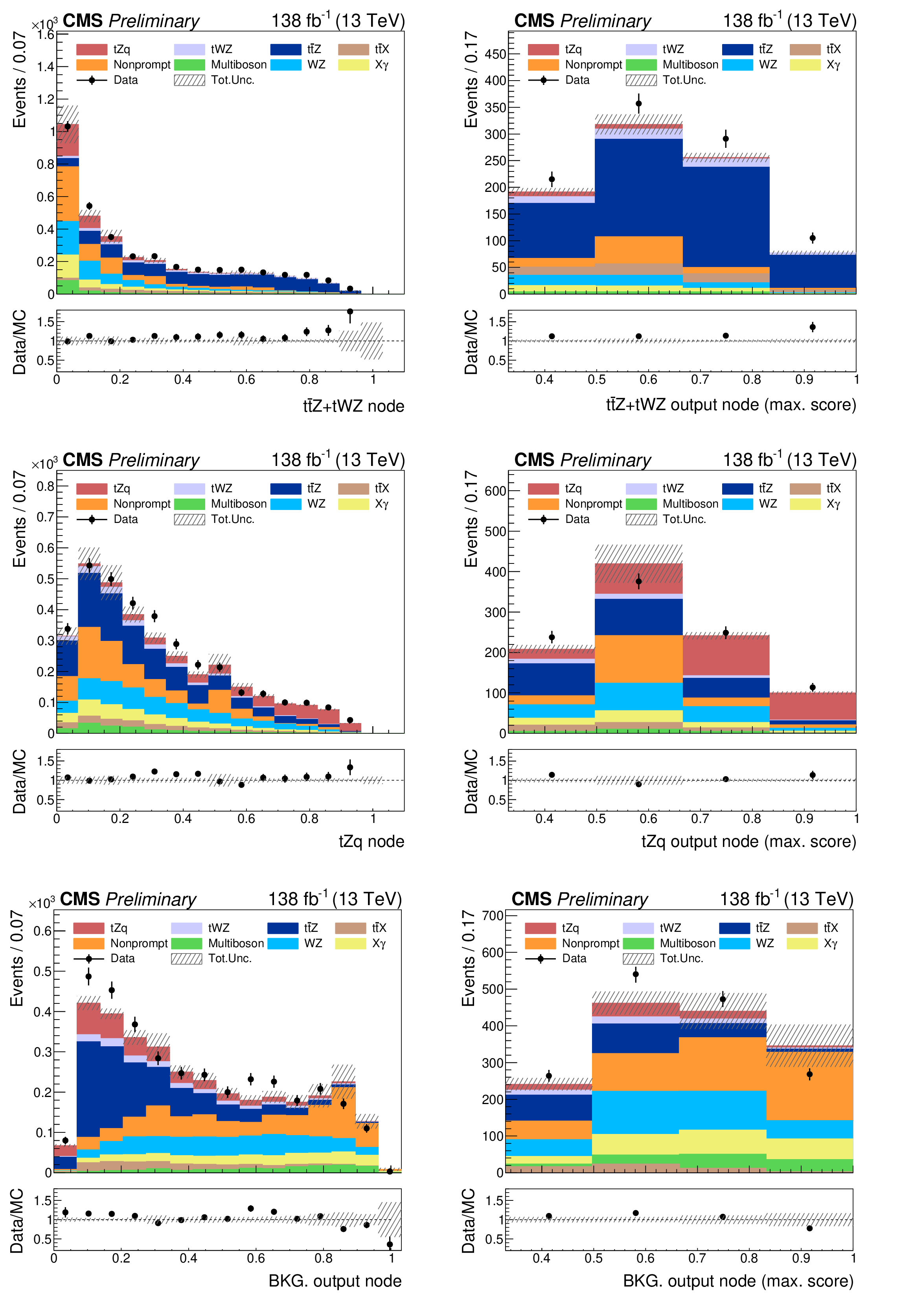
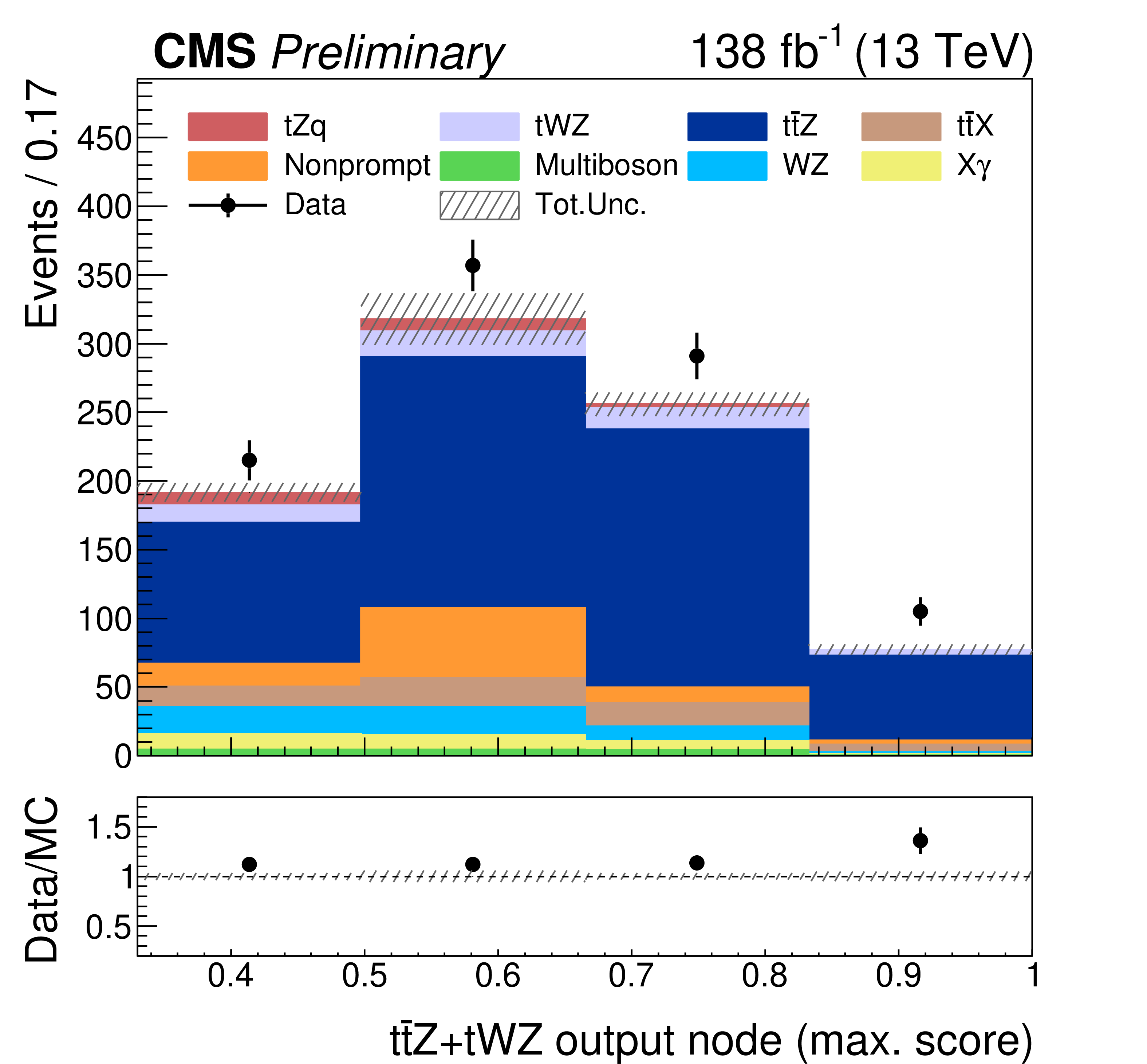
Figure 5:
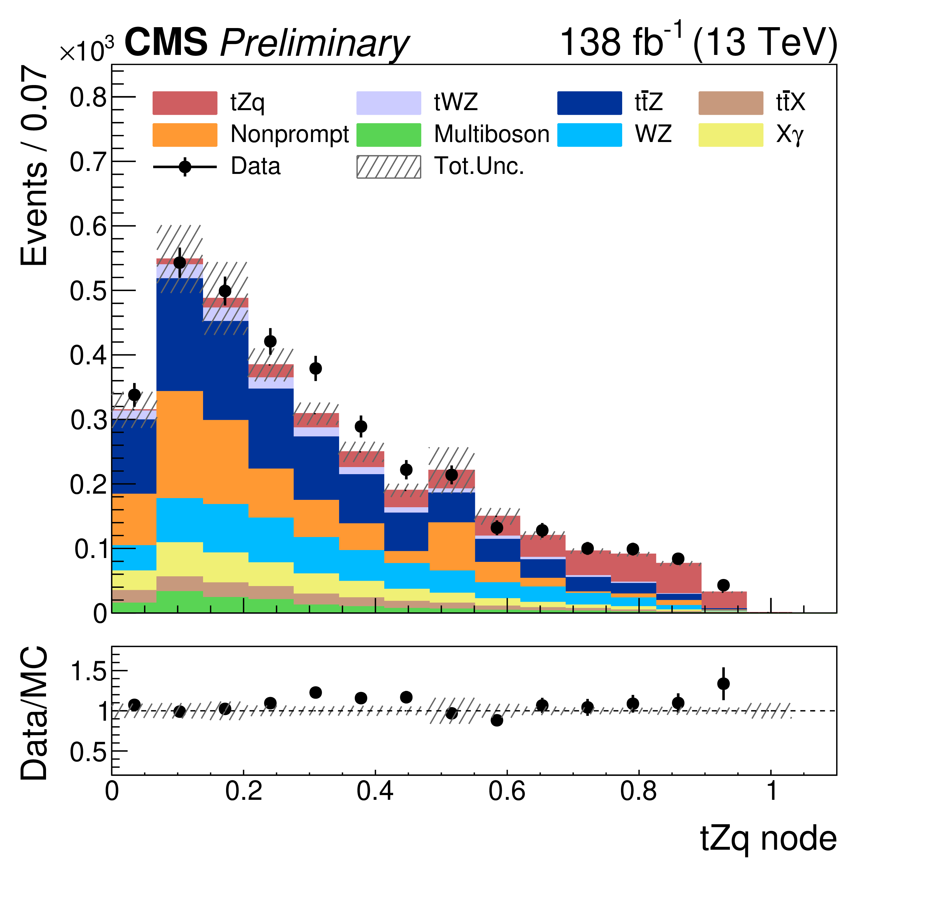
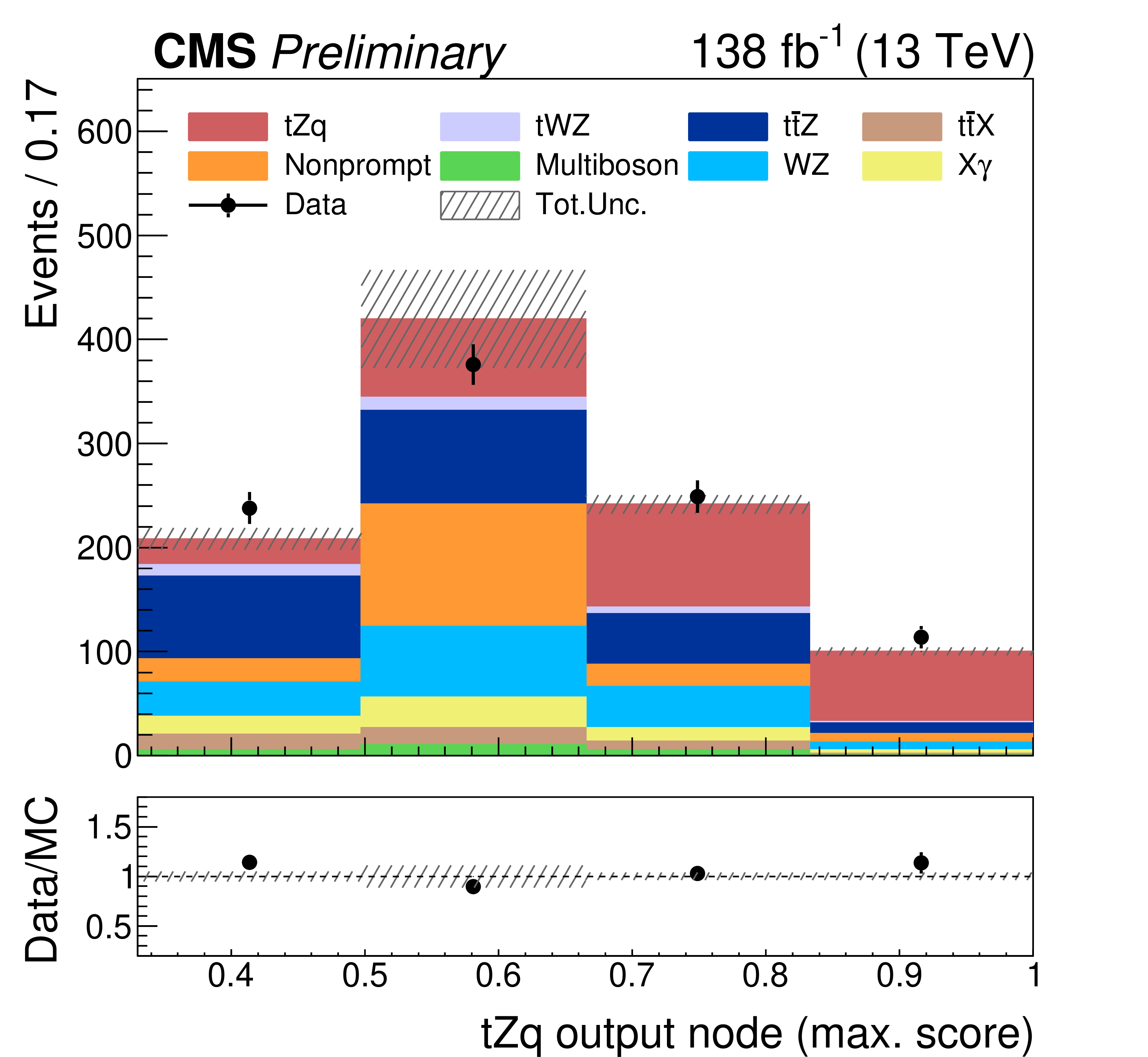
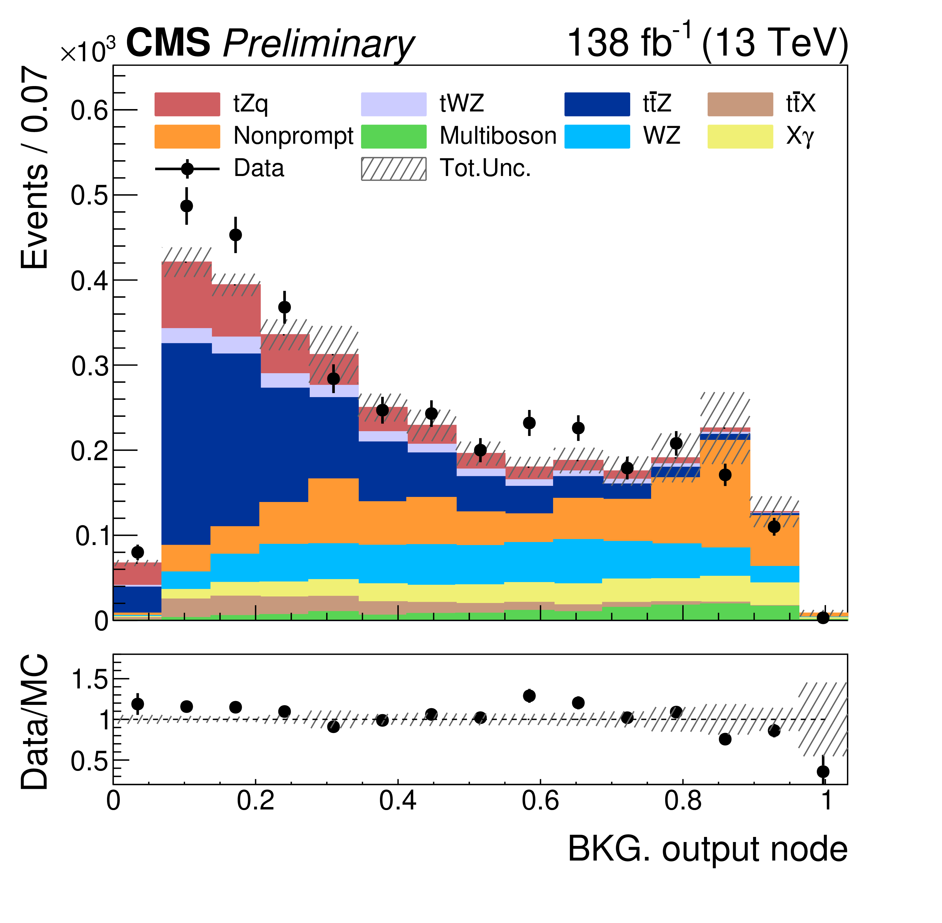
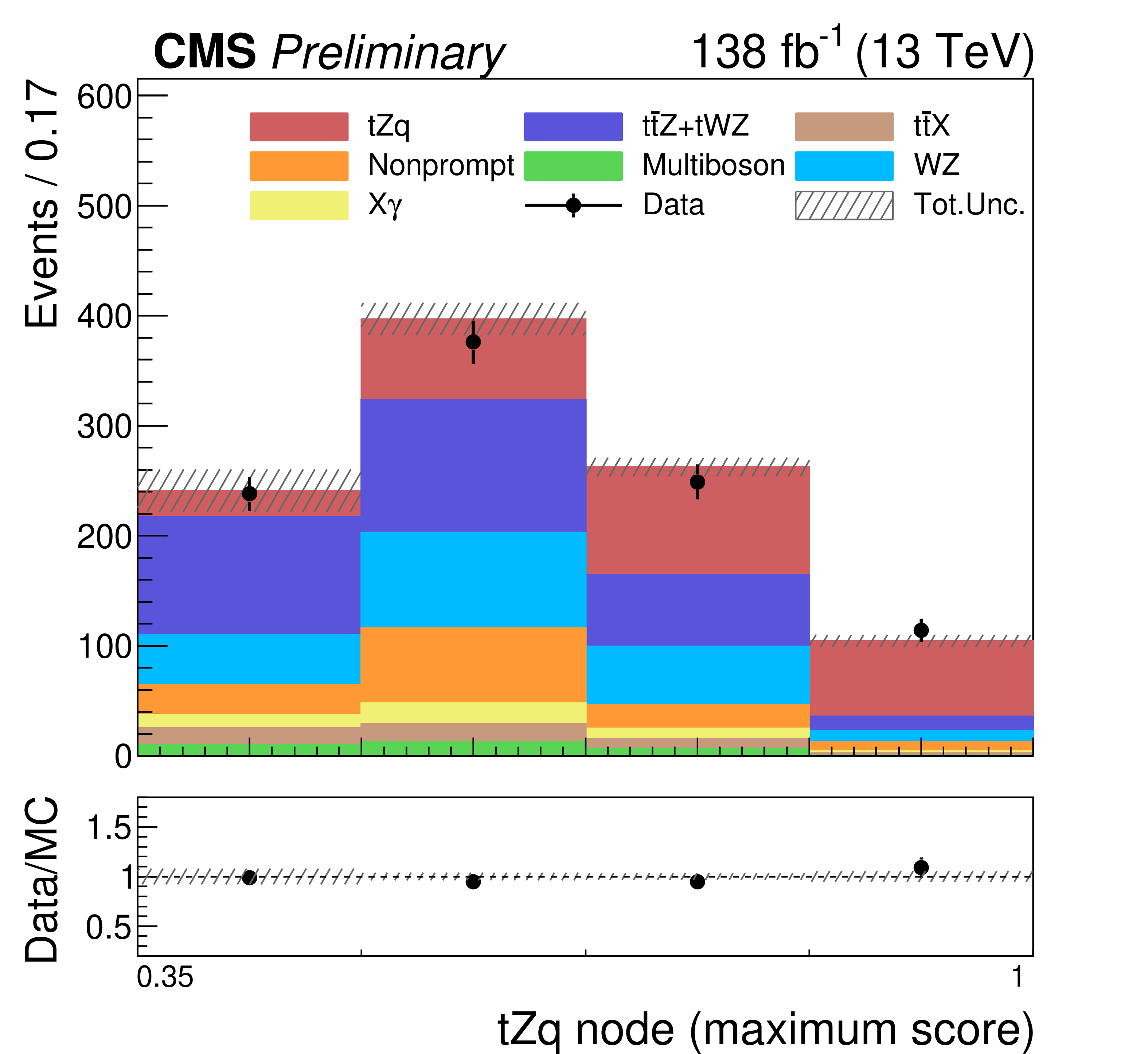
Distributions of output values in the three DNN output nodes for the sum of $ {\mathrm{t}\overline{\mathrm{t}}} \mathrm{Z} $ and $ \mathrm{t}\mathrm{W}\mathrm{Z} $ (upper), $ \mathrm{t}\mathrm{Z}\mathrm{q} $ (middle), and background (lower). In the left column, the inclusive distributions are shown, i.e.,, each selected event enters each of the output nodes. In the right column, each event enters exactly one of the three distributions, namely the one for which the output score is largest. These distributions, which by construction can not have entries below 1/3, are the templates that will be used for the signal extraction. Further details are described in the caption of Fig. 2. |

png pdf |
Figure 5-a:
Distributions of output values in the three DNN output nodes for the sum of $ {\mathrm{t}\overline{\mathrm{t}}} \mathrm{Z} $ and $ \mathrm{t}\mathrm{W}\mathrm{Z} $ (upper), $ \mathrm{t}\mathrm{Z}\mathrm{q} $ (middle), and background (lower). In the left column, the inclusive distributions are shown, i.e.,, each selected event enters each of the output nodes. In the right column, each event enters exactly one of the three distributions, namely the one for which the output score is largest. These distributions, which by construction can not have entries below 1/3, are the templates that will be used for the signal extraction. Further details are described in the caption of Fig. 2. |
png pdf |
Figure 5-b:
Distributions of output values in the three DNN output nodes for the sum of $ {\mathrm{t}\overline{\mathrm{t}}} \mathrm{Z} $ and $ \mathrm{t}\mathrm{W}\mathrm{Z} $ (upper), $ \mathrm{t}\mathrm{Z}\mathrm{q} $ (middle), and background (lower). In the left column, the inclusive distributions are shown, i.e.,, each selected event enters each of the output nodes. In the right column, each event enters exactly one of the three distributions, namely the one for which the output score is largest. These distributions, which by construction can not have entries below 1/3, are the templates that will be used for the signal extraction. Further details are described in the caption of Fig. 2. |
png pdf |
Figure 5-c:
Distributions of output values in the three DNN output nodes for the sum of $ {\mathrm{t}\overline{\mathrm{t}}} \mathrm{Z} $ and $ \mathrm{t}\mathrm{W}\mathrm{Z} $ (upper), $ \mathrm{t}\mathrm{Z}\mathrm{q} $ (middle), and background (lower). In the left column, the inclusive distributions are shown, i.e.,, each selected event enters each of the output nodes. In the right column, each event enters exactly one of the three distributions, namely the one for which the output score is largest. These distributions, which by construction can not have entries below 1/3, are the templates that will be used for the signal extraction. Further details are described in the caption of Fig. 2. |
png pdf |
Figure 5-d:
Distributions of output values in the three DNN output nodes for the sum of $ {\mathrm{t}\overline{\mathrm{t}}} \mathrm{Z} $ and $ \mathrm{t}\mathrm{W}\mathrm{Z} $ (upper), $ \mathrm{t}\mathrm{Z}\mathrm{q} $ (middle), and background (lower). In the left column, the inclusive distributions are shown, i.e.,, each selected event enters each of the output nodes. In the right column, each event enters exactly one of the three distributions, namely the one for which the output score is largest. These distributions, which by construction can not have entries below 1/3, are the templates that will be used for the signal extraction. Further details are described in the caption of Fig. 2. |
png pdf |
Figure 5-e:
Distributions of output values in the three DNN output nodes for the sum of $ {\mathrm{t}\overline{\mathrm{t}}} \mathrm{Z} $ and $ \mathrm{t}\mathrm{W}\mathrm{Z} $ (upper), $ \mathrm{t}\mathrm{Z}\mathrm{q} $ (middle), and background (lower). In the left column, the inclusive distributions are shown, i.e.,, each selected event enters each of the output nodes. In the right column, each event enters exactly one of the three distributions, namely the one for which the output score is largest. These distributions, which by construction can not have entries below 1/3, are the templates that will be used for the signal extraction. Further details are described in the caption of Fig. 2. |

png pdf |
Figure 5-f:
Distributions of output values in the three DNN output nodes for the sum of $ {\mathrm{t}\overline{\mathrm{t}}} \mathrm{Z} $ and $ \mathrm{t}\mathrm{W}\mathrm{Z} $ (upper), $ \mathrm{t}\mathrm{Z}\mathrm{q} $ (middle), and background (lower). In the left column, the inclusive distributions are shown, i.e.,, each selected event enters each of the output nodes. In the right column, each event enters exactly one of the three distributions, namely the one for which the output score is largest. These distributions, which by construction can not have entries below 1/3, are the templates that will be used for the signal extraction. Further details are described in the caption of Fig. 2. |

png pdf |
Figure 6:
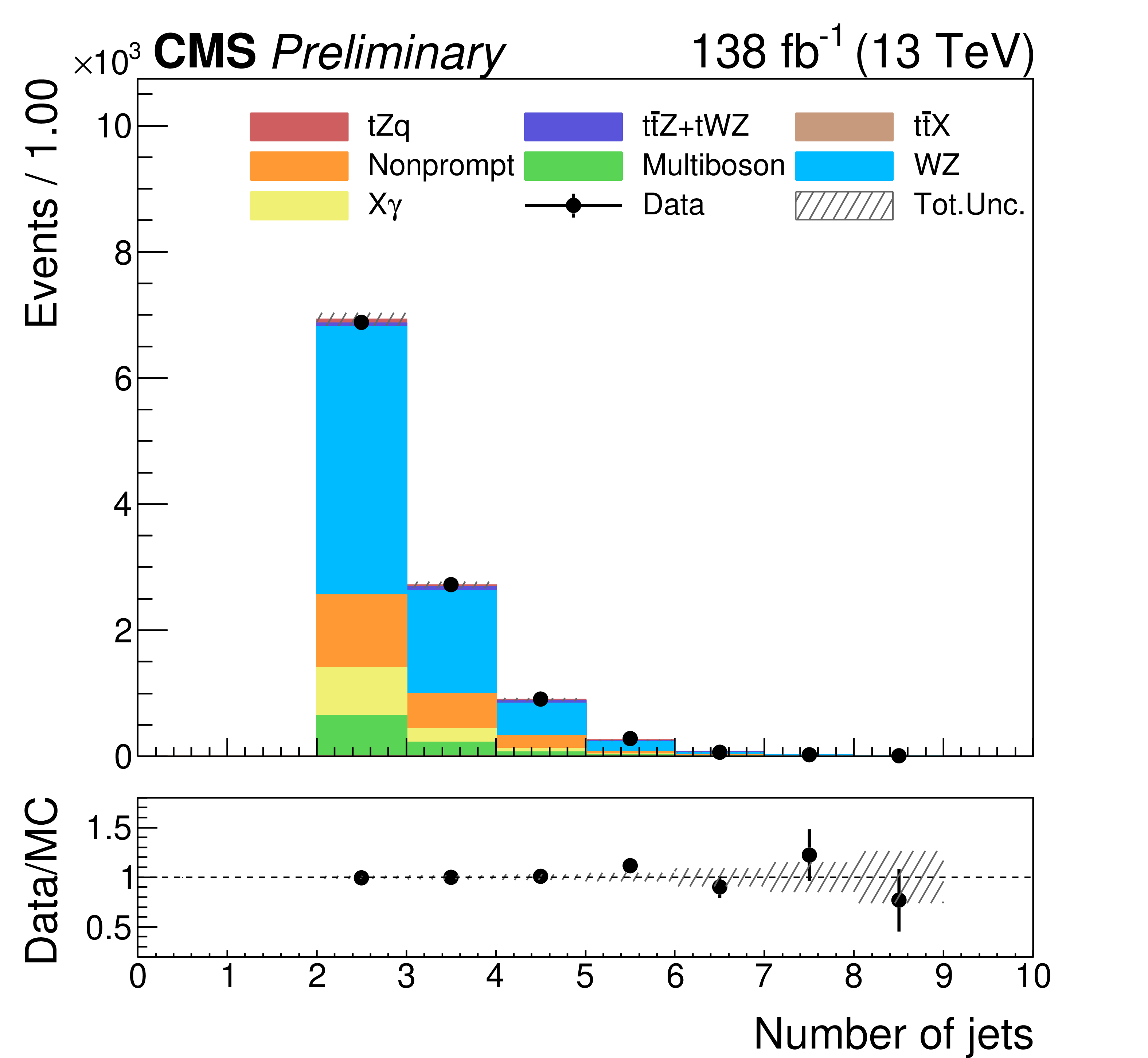
Distributions of the b-jet multiplicity in the four lepton region (left) and the jet multiplicity in the zero b-jet control region (right). These distributions are added to the fit for the inclusive measurements. |

png pdf |
Figure 6-a:
Distributions of the b-jet multiplicity in the four lepton region (left) and the jet multiplicity in the zero b-jet control region (right). These distributions are added to the fit for the inclusive measurements. |

png pdf |
Figure 6-b:
Distributions of the b-jet multiplicity in the four lepton region (left) and the jet multiplicity in the zero b-jet control region (right). These distributions are added to the fit for the inclusive measurements. |

png pdf |
Figure 7:
Likelihood scan of the two measured inclusive cross sections normalized to the SM predictions $ \mu_{{\mathrm{t}\overline{\mathrm{t}}} \mathrm{Z}+\mathrm{t}\mathrm{W}\mathrm{Z}} $ and $ \mu_{\mathrm{t}\mathrm{Z}\mathrm{q}} $. |

png pdf |
Figure 8:
Postfit distributions of the b-jet multiplicity in events with four leptons (upper left) and the jet multiplicity distribution in events with zero b jets (upper right). The corresponding prefit distributions are presented in Fig. 6. Postfit distributions in the output nodes for $ \mathrm{t}\mathrm{Z}\mathrm{q} $ (middle left), $ {\mathrm{t}\overline{\mathrm{t}}} \mathrm{Z}+\mathrm{t}\mathrm{W}\mathrm{Z} $ (middle right), and the background (lower). The corresponding prefit distributions are presented in the right column of Fig. 5. |

png pdf |
Figure 8-a:
Postfit distributions of the b-jet multiplicity in events with four leptons (upper left) and the jet multiplicity distribution in events with zero b jets (upper right). The corresponding prefit distributions are presented in Fig. 6. Postfit distributions in the output nodes for $ \mathrm{t}\mathrm{Z}\mathrm{q} $ (middle left), $ {\mathrm{t}\overline{\mathrm{t}}} \mathrm{Z}+\mathrm{t}\mathrm{W}\mathrm{Z} $ (middle right), and the background (lower). The corresponding prefit distributions are presented in the right column of Fig. 5. |
png pdf |
Figure 8-b:
Postfit distributions of the b-jet multiplicity in events with four leptons (upper left) and the jet multiplicity distribution in events with zero b jets (upper right). The corresponding prefit distributions are presented in Fig. 6. Postfit distributions in the output nodes for $ \mathrm{t}\mathrm{Z}\mathrm{q} $ (middle left), $ {\mathrm{t}\overline{\mathrm{t}}} \mathrm{Z}+\mathrm{t}\mathrm{W}\mathrm{Z} $ (middle right), and the background (lower). The corresponding prefit distributions are presented in the right column of Fig. 5. |
png pdf |
Figure 8-c:
Postfit distributions of the b-jet multiplicity in events with four leptons (upper left) and the jet multiplicity distribution in events with zero b jets (upper right). The corresponding prefit distributions are presented in Fig. 6. Postfit distributions in the output nodes for $ \mathrm{t}\mathrm{Z}\mathrm{q} $ (middle left), $ {\mathrm{t}\overline{\mathrm{t}}} \mathrm{Z}+\mathrm{t}\mathrm{W}\mathrm{Z} $ (middle right), and the background (lower). The corresponding prefit distributions are presented in the right column of Fig. 5. |

png pdf |
Figure 8-d:
Postfit distributions of the b-jet multiplicity in events with four leptons (upper left) and the jet multiplicity distribution in events with zero b jets (upper right). The corresponding prefit distributions are presented in Fig. 6. Postfit distributions in the output nodes for $ \mathrm{t}\mathrm{Z}\mathrm{q} $ (middle left), $ {\mathrm{t}\overline{\mathrm{t}}} \mathrm{Z}+\mathrm{t}\mathrm{W}\mathrm{Z} $ (middle right), and the background (lower). The corresponding prefit distributions are presented in the right column of Fig. 5. |

png pdf |
Figure 8-e:
Postfit distributions of the b-jet multiplicity in events with four leptons (upper left) and the jet multiplicity distribution in events with zero b jets (upper right). The corresponding prefit distributions are presented in Fig. 6. Postfit distributions in the output nodes for $ \mathrm{t}\mathrm{Z}\mathrm{q} $ (middle left), $ {\mathrm{t}\overline{\mathrm{t}}} \mathrm{Z}+\mathrm{t}\mathrm{W}\mathrm{Z} $ (middle right), and the background (lower). The corresponding prefit distributions are presented in the right column of Fig. 5. |

png pdf |
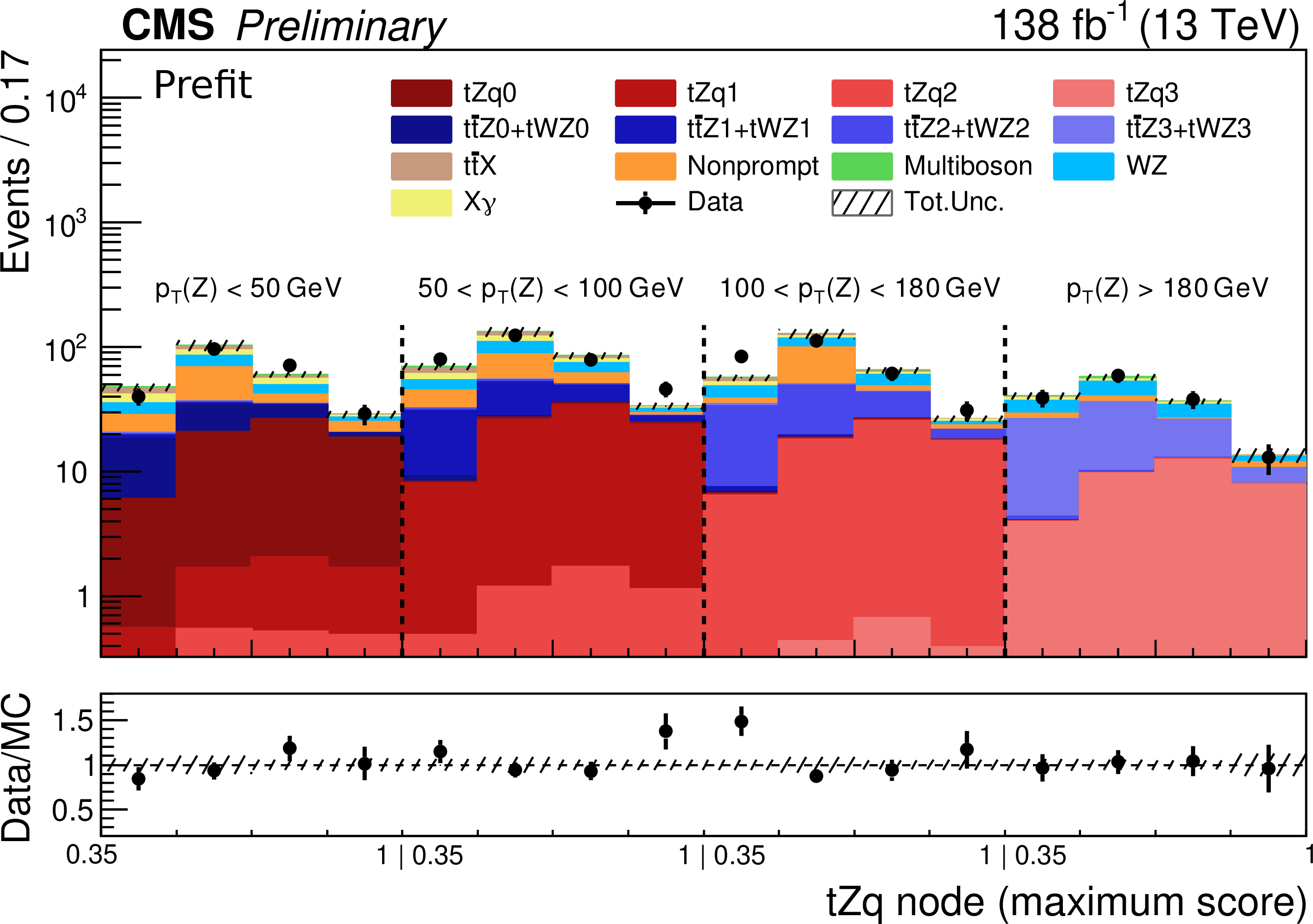
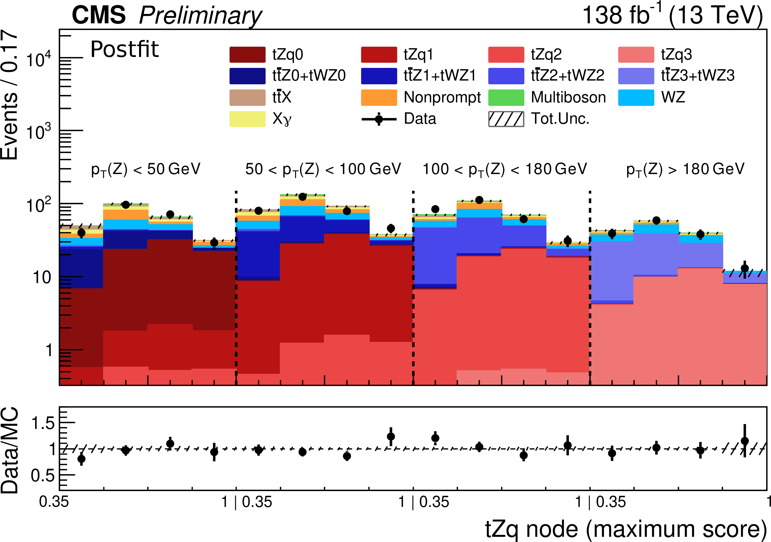
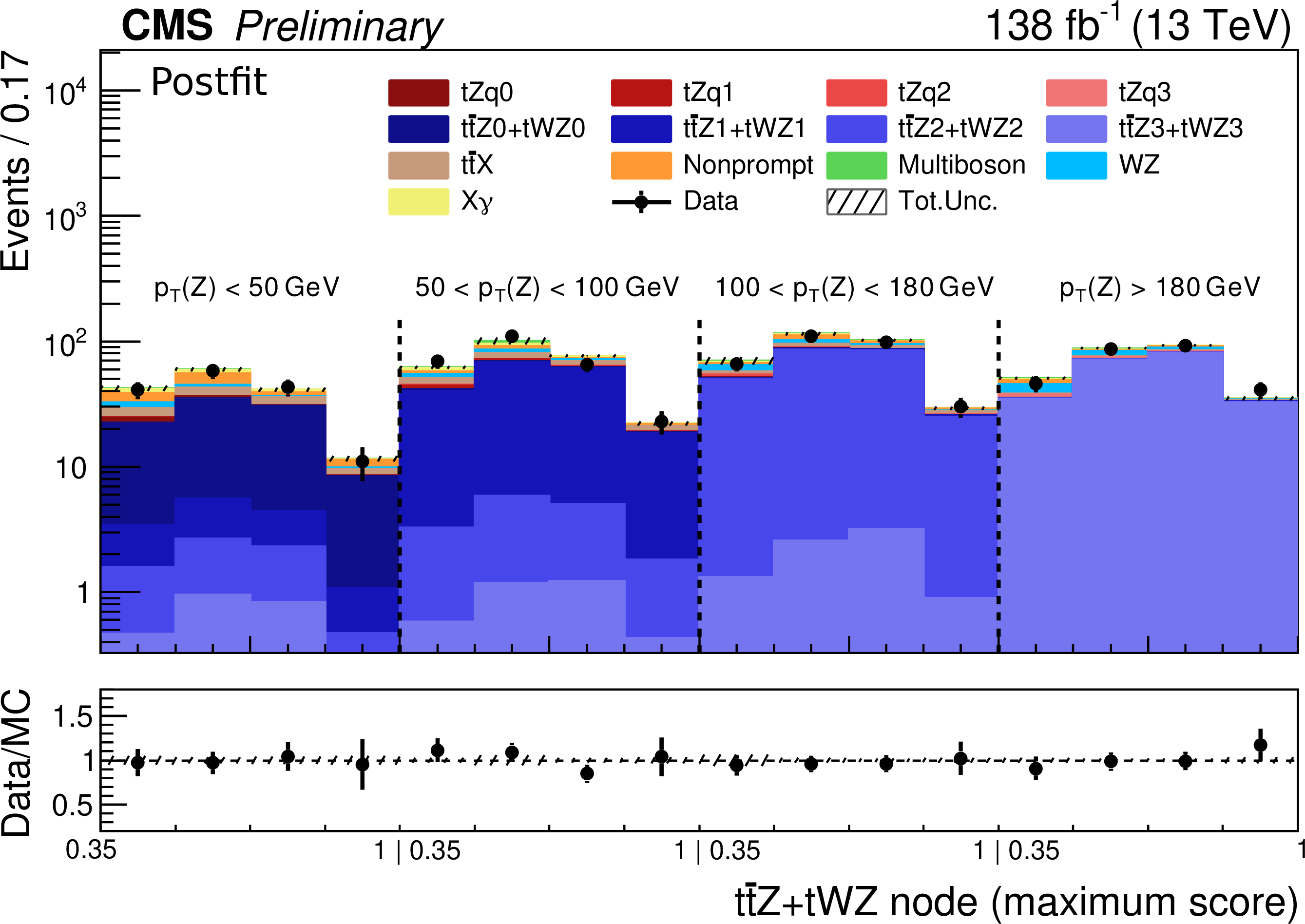
Figure 9:
Prefit (upper) and postfit (lower) output node distributions for $ \mathrm{t}\mathrm{Z}\mathrm{q} $ (left) and the sum of $ {\mathrm{t}\overline{\mathrm{t}}} \mathrm{Z} $ and $ \mathrm{t}\mathrm{W}\mathrm{Z} $ (right). Separate templates are shown for each bin of reconstructed $ p_{\mathrm{T}}(\mathrm{Z}) $. The signal samples are further split into four components each, according to the generator-level bins of $ p_{\mathrm{T}}(\mathrm{Z}) $. In the legend, the numerical suffixes (0, 1, 2, 3) represent bin indices. |
png pdf |
Figure 9-a:
Prefit (upper) and postfit (lower) output node distributions for $ \mathrm{t}\mathrm{Z}\mathrm{q} $ (left) and the sum of $ {\mathrm{t}\overline{\mathrm{t}}} \mathrm{Z} $ and $ \mathrm{t}\mathrm{W}\mathrm{Z} $ (right). Separate templates are shown for each bin of reconstructed $ p_{\mathrm{T}}(\mathrm{Z}) $. The signal samples are further split into four components each, according to the generator-level bins of $ p_{\mathrm{T}}(\mathrm{Z}) $. In the legend, the numerical suffixes (0, 1, 2, 3) represent bin indices. |

png pdf |
Figure 9-b:
Prefit (upper) and postfit (lower) output node distributions for $ \mathrm{t}\mathrm{Z}\mathrm{q} $ (left) and the sum of $ {\mathrm{t}\overline{\mathrm{t}}} \mathrm{Z} $ and $ \mathrm{t}\mathrm{W}\mathrm{Z} $ (right). Separate templates are shown for each bin of reconstructed $ p_{\mathrm{T}}(\mathrm{Z}) $. The signal samples are further split into four components each, according to the generator-level bins of $ p_{\mathrm{T}}(\mathrm{Z}) $. In the legend, the numerical suffixes (0, 1, 2, 3) represent bin indices. |
png pdf |
Figure 9-c:
Prefit (upper) and postfit (lower) output node distributions for $ \mathrm{t}\mathrm{Z}\mathrm{q} $ (left) and the sum of $ {\mathrm{t}\overline{\mathrm{t}}} \mathrm{Z} $ and $ \mathrm{t}\mathrm{W}\mathrm{Z} $ (right). Separate templates are shown for each bin of reconstructed $ p_{\mathrm{T}}(\mathrm{Z}) $. The signal samples are further split into four components each, according to the generator-level bins of $ p_{\mathrm{T}}(\mathrm{Z}) $. In the legend, the numerical suffixes (0, 1, 2, 3) represent bin indices. |
png pdf |
Figure 9-d:
Prefit (upper) and postfit (lower) output node distributions for $ \mathrm{t}\mathrm{Z}\mathrm{q} $ (left) and the sum of $ {\mathrm{t}\overline{\mathrm{t}}} \mathrm{Z} $ and $ \mathrm{t}\mathrm{W}\mathrm{Z} $ (right). Separate templates are shown for each bin of reconstructed $ p_{\mathrm{T}}(\mathrm{Z}) $. The signal samples are further split into four components each, according to the generator-level bins of $ p_{\mathrm{T}}(\mathrm{Z}) $. In the legend, the numerical suffixes (0, 1, 2, 3) represent bin indices. |

png pdf |
Figure 10:
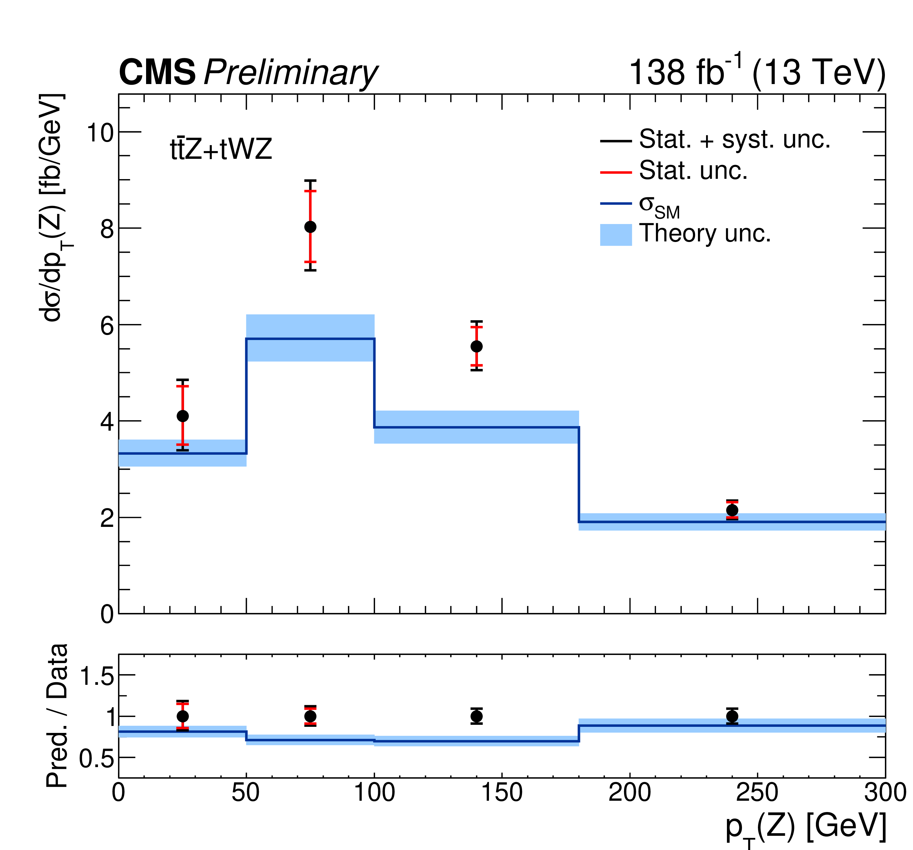
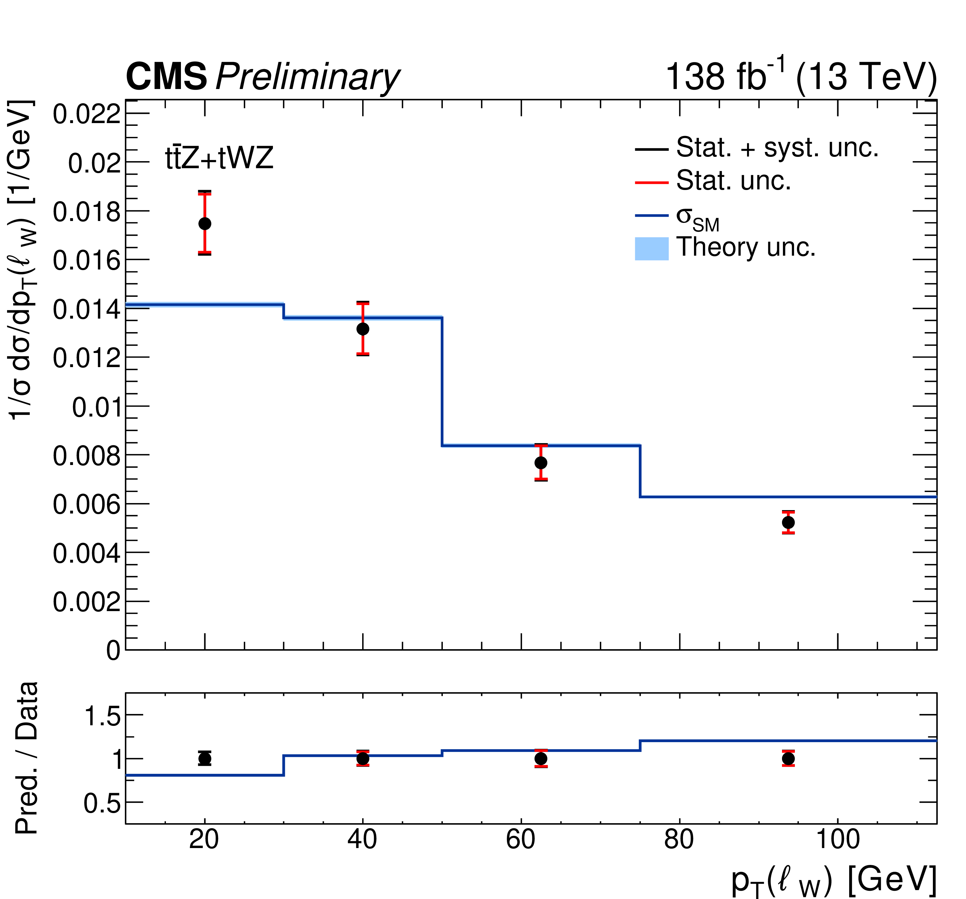
Differential cross sections for $ \mathrm{t}\mathrm{Z}\mathrm{q} $ (left column) and the sum of $ {\mathrm{t}\overline{\mathrm{t}}} \mathrm{Z} $ and $ \mathrm{t}\mathrm{W}\mathrm{Z} $ (right column) as a function of $ p_{\mathrm{T}}(\mathrm{Z}) $ (upper), $ p_{\mathrm{T}}(\ell_\mathrm{W}) $ (middle), and $ \Delta \phi(\ell^{+},\,\ell^{-}) $ (lower). The inner (outer) error bars indicate the statistical (total) uncertainty, while the blue area refers to the uncertainty on the theory prediction. |

png pdf |
Figure 10-a:
Differential cross sections for $ \mathrm{t}\mathrm{Z}\mathrm{q} $ (left column) and the sum of $ {\mathrm{t}\overline{\mathrm{t}}} \mathrm{Z} $ and $ \mathrm{t}\mathrm{W}\mathrm{Z} $ (right column) as a function of $ p_{\mathrm{T}}(\mathrm{Z}) $ (upper), $ p_{\mathrm{T}}(\ell_\mathrm{W}) $ (middle), and $ \Delta \phi(\ell^{+},\,\ell^{-}) $ (lower). The inner (outer) error bars indicate the statistical (total) uncertainty, while the blue area refers to the uncertainty on the theory prediction. |
png pdf |
Figure 10-b:
Differential cross sections for $ \mathrm{t}\mathrm{Z}\mathrm{q} $ (left column) and the sum of $ {\mathrm{t}\overline{\mathrm{t}}} \mathrm{Z} $ and $ \mathrm{t}\mathrm{W}\mathrm{Z} $ (right column) as a function of $ p_{\mathrm{T}}(\mathrm{Z}) $ (upper), $ p_{\mathrm{T}}(\ell_\mathrm{W}) $ (middle), and $ \Delta \phi(\ell^{+},\,\ell^{-}) $ (lower). The inner (outer) error bars indicate the statistical (total) uncertainty, while the blue area refers to the uncertainty on the theory prediction. |

png pdf |
Figure 10-c:
Differential cross sections for $ \mathrm{t}\mathrm{Z}\mathrm{q} $ (left column) and the sum of $ {\mathrm{t}\overline{\mathrm{t}}} \mathrm{Z} $ and $ \mathrm{t}\mathrm{W}\mathrm{Z} $ (right column) as a function of $ p_{\mathrm{T}}(\mathrm{Z}) $ (upper), $ p_{\mathrm{T}}(\ell_\mathrm{W}) $ (middle), and $ \Delta \phi(\ell^{+},\,\ell^{-}) $ (lower). The inner (outer) error bars indicate the statistical (total) uncertainty, while the blue area refers to the uncertainty on the theory prediction. |

png pdf |
Figure 10-d:
Differential cross sections for $ \mathrm{t}\mathrm{Z}\mathrm{q} $ (left column) and the sum of $ {\mathrm{t}\overline{\mathrm{t}}} \mathrm{Z} $ and $ \mathrm{t}\mathrm{W}\mathrm{Z} $ (right column) as a function of $ p_{\mathrm{T}}(\mathrm{Z}) $ (upper), $ p_{\mathrm{T}}(\ell_\mathrm{W}) $ (middle), and $ \Delta \phi(\ell^{+},\,\ell^{-}) $ (lower). The inner (outer) error bars indicate the statistical (total) uncertainty, while the blue area refers to the uncertainty on the theory prediction. |

png pdf |
Figure 10-e:
Differential cross sections for $ \mathrm{t}\mathrm{Z}\mathrm{q} $ (left column) and the sum of $ {\mathrm{t}\overline{\mathrm{t}}} \mathrm{Z} $ and $ \mathrm{t}\mathrm{W}\mathrm{Z} $ (right column) as a function of $ p_{\mathrm{T}}(\mathrm{Z}) $ (upper), $ p_{\mathrm{T}}(\ell_\mathrm{W}) $ (middle), and $ \Delta \phi(\ell^{+},\,\ell^{-}) $ (lower). The inner (outer) error bars indicate the statistical (total) uncertainty, while the blue area refers to the uncertainty on the theory prediction. |

png pdf |
Figure 10-f:
Differential cross sections for $ \mathrm{t}\mathrm{Z}\mathrm{q} $ (left column) and the sum of $ {\mathrm{t}\overline{\mathrm{t}}} \mathrm{Z} $ and $ \mathrm{t}\mathrm{W}\mathrm{Z} $ (right column) as a function of $ p_{\mathrm{T}}(\mathrm{Z}) $ (upper), $ p_{\mathrm{T}}(\ell_\mathrm{W}) $ (middle), and $ \Delta \phi(\ell^{+},\,\ell^{-}) $ (lower). The inner (outer) error bars indicate the statistical (total) uncertainty, while the blue area refers to the uncertainty on the theory prediction. |

png pdf |
Figure 11:
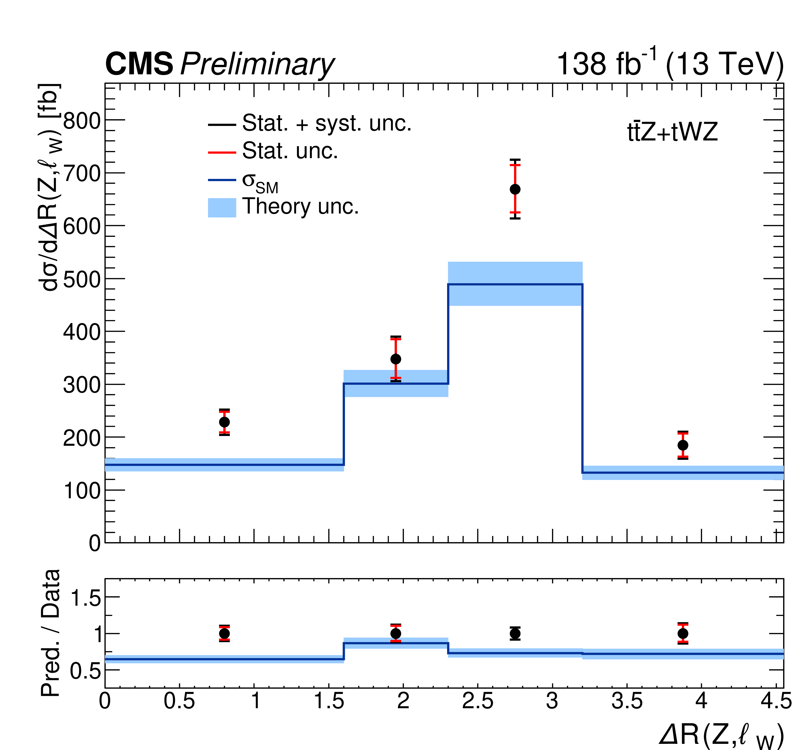
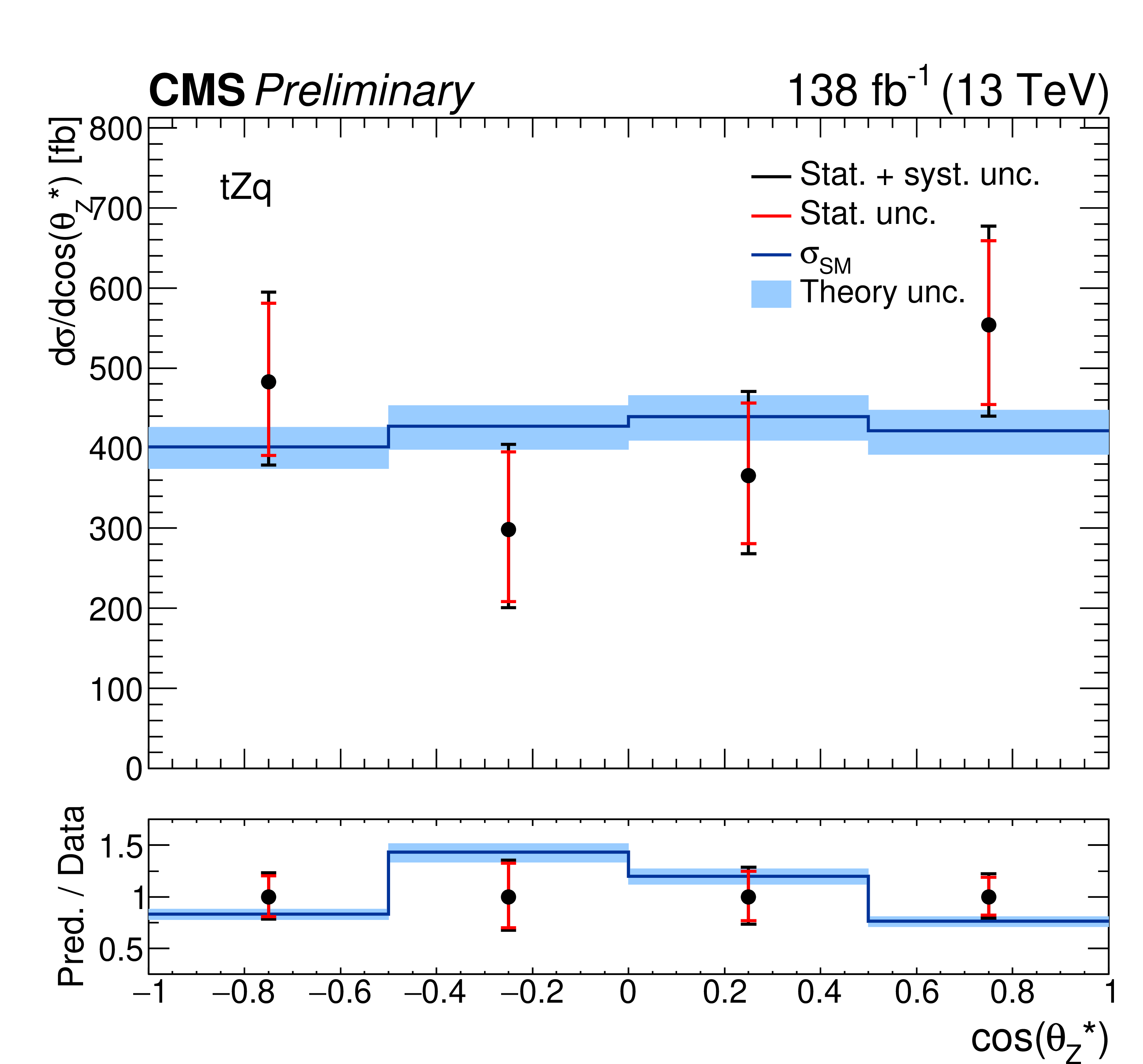
Differential cross sections for $ \mathrm{t}\mathrm{Z}\mathrm{q} $ (left column) and the sum of $ {\mathrm{t}\overline{\mathrm{t}}} \mathrm{Z} $ and $ \mathrm{t}\mathrm{W}\mathrm{Z} $ (right column) differential cross sections as a function of $ \Delta R $ (Z,t) (upper), and $ \cos\theta^\ast_{\mathrm{Z}} $ (lower). The inner (outer) error bars indicate the statistical (total) uncertainty, while the blue area refers to the uncertainty on the theory prediction. |

png pdf |
Figure 11-a:
Differential cross sections for $ \mathrm{t}\mathrm{Z}\mathrm{q} $ (left column) and the sum of $ {\mathrm{t}\overline{\mathrm{t}}} \mathrm{Z} $ and $ \mathrm{t}\mathrm{W}\mathrm{Z} $ (right column) differential cross sections as a function of $ \Delta R $ (Z,t) (upper), and $ \cos\theta^\ast_{\mathrm{Z}} $ (lower). The inner (outer) error bars indicate the statistical (total) uncertainty, while the blue area refers to the uncertainty on the theory prediction. |
png pdf |
Figure 11-b:
Differential cross sections for $ \mathrm{t}\mathrm{Z}\mathrm{q} $ (left column) and the sum of $ {\mathrm{t}\overline{\mathrm{t}}} \mathrm{Z} $ and $ \mathrm{t}\mathrm{W}\mathrm{Z} $ (right column) differential cross sections as a function of $ \Delta R $ (Z,t) (upper), and $ \cos\theta^\ast_{\mathrm{Z}} $ (lower). The inner (outer) error bars indicate the statistical (total) uncertainty, while the blue area refers to the uncertainty on the theory prediction. |
png pdf |
Figure 11-c:
Differential cross sections for $ \mathrm{t}\mathrm{Z}\mathrm{q} $ (left column) and the sum of $ {\mathrm{t}\overline{\mathrm{t}}} \mathrm{Z} $ and $ \mathrm{t}\mathrm{W}\mathrm{Z} $ (right column) differential cross sections as a function of $ \Delta R $ (Z,t) (upper), and $ \cos\theta^\ast_{\mathrm{Z}} $ (lower). The inner (outer) error bars indicate the statistical (total) uncertainty, while the blue area refers to the uncertainty on the theory prediction. |

png pdf |
Figure 11-d:
Differential cross sections for $ \mathrm{t}\mathrm{Z}\mathrm{q} $ (left column) and the sum of $ {\mathrm{t}\overline{\mathrm{t}}} \mathrm{Z} $ and $ \mathrm{t}\mathrm{W}\mathrm{Z} $ (right column) differential cross sections as a function of $ \Delta R $ (Z,t) (upper), and $ \cos\theta^\ast_{\mathrm{Z}} $ (lower). The inner (outer) error bars indicate the statistical (total) uncertainty, while the blue area refers to the uncertainty on the theory prediction. |

png pdf |
Figure 12:
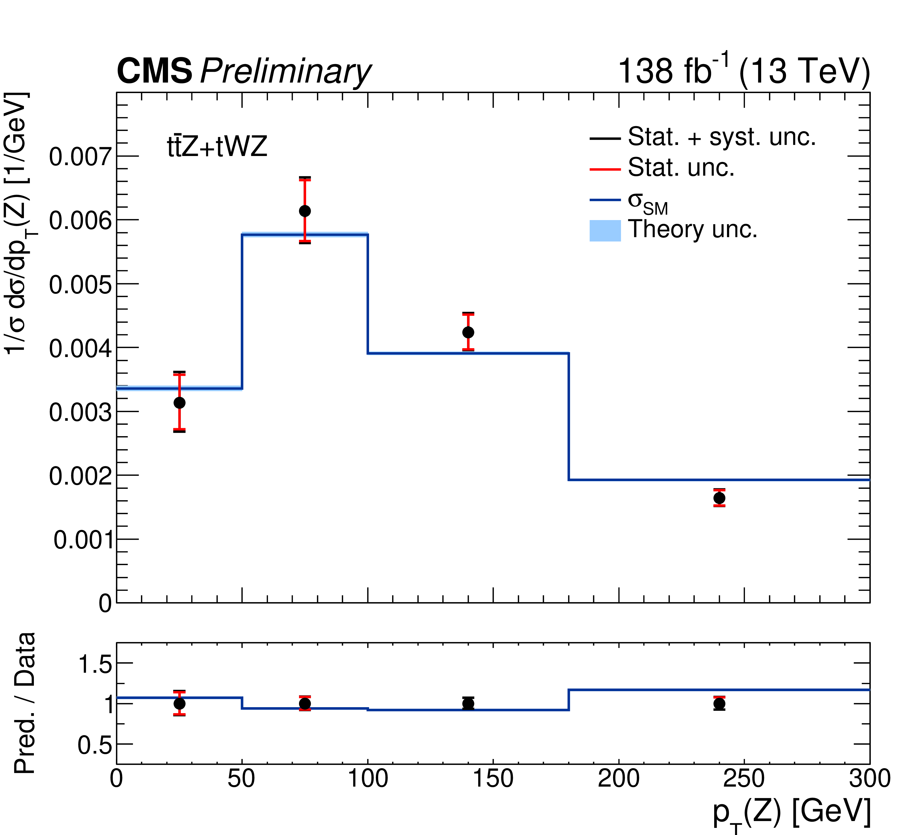
Normalized differential cross sections for $ \mathrm{t}\mathrm{Z}\mathrm{q} $ (left column) and the sum of $ {\mathrm{t}\overline{\mathrm{t}}} \mathrm{Z} $ and $ \mathrm{t}\mathrm{W}\mathrm{Z} $ (right column) as a function of $ p_{\mathrm{T}}(\mathrm{Z}) $ (upper), $ p_{\mathrm{T}}(\ell_\mathrm{W}) $ (middle), and $ \Delta \phi(\ell^{+},\,\ell^{-}) $ (lower). The inner (outer) error bars indicate the statistical (total) uncertainty, while the blue area refers to the uncertainty on the theory prediction. |

png pdf |
Figure 12-a:
Normalized differential cross sections for $ \mathrm{t}\mathrm{Z}\mathrm{q} $ (left column) and the sum of $ {\mathrm{t}\overline{\mathrm{t}}} \mathrm{Z} $ and $ \mathrm{t}\mathrm{W}\mathrm{Z} $ (right column) as a function of $ p_{\mathrm{T}}(\mathrm{Z}) $ (upper), $ p_{\mathrm{T}}(\ell_\mathrm{W}) $ (middle), and $ \Delta \phi(\ell^{+},\,\ell^{-}) $ (lower). The inner (outer) error bars indicate the statistical (total) uncertainty, while the blue area refers to the uncertainty on the theory prediction. |
png pdf |
Figure 12-b:
Normalized differential cross sections for $ \mathrm{t}\mathrm{Z}\mathrm{q} $ (left column) and the sum of $ {\mathrm{t}\overline{\mathrm{t}}} \mathrm{Z} $ and $ \mathrm{t}\mathrm{W}\mathrm{Z} $ (right column) as a function of $ p_{\mathrm{T}}(\mathrm{Z}) $ (upper), $ p_{\mathrm{T}}(\ell_\mathrm{W}) $ (middle), and $ \Delta \phi(\ell^{+},\,\ell^{-}) $ (lower). The inner (outer) error bars indicate the statistical (total) uncertainty, while the blue area refers to the uncertainty on the theory prediction. |

png pdf |
Figure 12-c:
Normalized differential cross sections for $ \mathrm{t}\mathrm{Z}\mathrm{q} $ (left column) and the sum of $ {\mathrm{t}\overline{\mathrm{t}}} \mathrm{Z} $ and $ \mathrm{t}\mathrm{W}\mathrm{Z} $ (right column) as a function of $ p_{\mathrm{T}}(\mathrm{Z}) $ (upper), $ p_{\mathrm{T}}(\ell_\mathrm{W}) $ (middle), and $ \Delta \phi(\ell^{+},\,\ell^{-}) $ (lower). The inner (outer) error bars indicate the statistical (total) uncertainty, while the blue area refers to the uncertainty on the theory prediction. |
png pdf |
Figure 12-d:
Normalized differential cross sections for $ \mathrm{t}\mathrm{Z}\mathrm{q} $ (left column) and the sum of $ {\mathrm{t}\overline{\mathrm{t}}} \mathrm{Z} $ and $ \mathrm{t}\mathrm{W}\mathrm{Z} $ (right column) as a function of $ p_{\mathrm{T}}(\mathrm{Z}) $ (upper), $ p_{\mathrm{T}}(\ell_\mathrm{W}) $ (middle), and $ \Delta \phi(\ell^{+},\,\ell^{-}) $ (lower). The inner (outer) error bars indicate the statistical (total) uncertainty, while the blue area refers to the uncertainty on the theory prediction. |

png pdf |
Figure 12-e:
Normalized differential cross sections for $ \mathrm{t}\mathrm{Z}\mathrm{q} $ (left column) and the sum of $ {\mathrm{t}\overline{\mathrm{t}}} \mathrm{Z} $ and $ \mathrm{t}\mathrm{W}\mathrm{Z} $ (right column) as a function of $ p_{\mathrm{T}}(\mathrm{Z}) $ (upper), $ p_{\mathrm{T}}(\ell_\mathrm{W}) $ (middle), and $ \Delta \phi(\ell^{+},\,\ell^{-}) $ (lower). The inner (outer) error bars indicate the statistical (total) uncertainty, while the blue area refers to the uncertainty on the theory prediction. |

png pdf |
Figure 12-f:
Normalized differential cross sections for $ \mathrm{t}\mathrm{Z}\mathrm{q} $ (left column) and the sum of $ {\mathrm{t}\overline{\mathrm{t}}} \mathrm{Z} $ and $ \mathrm{t}\mathrm{W}\mathrm{Z} $ (right column) as a function of $ p_{\mathrm{T}}(\mathrm{Z}) $ (upper), $ p_{\mathrm{T}}(\ell_\mathrm{W}) $ (middle), and $ \Delta \phi(\ell^{+},\,\ell^{-}) $ (lower). The inner (outer) error bars indicate the statistical (total) uncertainty, while the blue area refers to the uncertainty on the theory prediction. |

png pdf |
Figure 13:
Normalized differential cross sections for $ \mathrm{t}\mathrm{Z}\mathrm{q} $ (left column) and the sum of $ {\mathrm{t}\overline{\mathrm{t}}} \mathrm{Z} $ and $ \mathrm{t}\mathrm{W}\mathrm{Z} $ (right column) differential cross sections as a function of $ \Delta R $ (Z,t) (upper), and $ \cos\theta^\ast_{\mathrm{Z}} $ (lower). The inner (outer) error bars indicate the statistical (total) uncertainty, while the blue area refers to the uncertainty on the theory prediction. |

png pdf |
Figure 13-a:
Normalized differential cross sections for $ \mathrm{t}\mathrm{Z}\mathrm{q} $ (left column) and the sum of $ {\mathrm{t}\overline{\mathrm{t}}} \mathrm{Z} $ and $ \mathrm{t}\mathrm{W}\mathrm{Z} $ (right column) differential cross sections as a function of $ \Delta R $ (Z,t) (upper), and $ \cos\theta^\ast_{\mathrm{Z}} $ (lower). The inner (outer) error bars indicate the statistical (total) uncertainty, while the blue area refers to the uncertainty on the theory prediction. |

png pdf |
Figure 13-b:
Normalized differential cross sections for $ \mathrm{t}\mathrm{Z}\mathrm{q} $ (left column) and the sum of $ {\mathrm{t}\overline{\mathrm{t}}} \mathrm{Z} $ and $ \mathrm{t}\mathrm{W}\mathrm{Z} $ (right column) differential cross sections as a function of $ \Delta R $ (Z,t) (upper), and $ \cos\theta^\ast_{\mathrm{Z}} $ (lower). The inner (outer) error bars indicate the statistical (total) uncertainty, while the blue area refers to the uncertainty on the theory prediction. |

png pdf |
Figure 13-c:
Normalized differential cross sections for $ \mathrm{t}\mathrm{Z}\mathrm{q} $ (left column) and the sum of $ {\mathrm{t}\overline{\mathrm{t}}} \mathrm{Z} $ and $ \mathrm{t}\mathrm{W}\mathrm{Z} $ (right column) differential cross sections as a function of $ \Delta R $ (Z,t) (upper), and $ \cos\theta^\ast_{\mathrm{Z}} $ (lower). The inner (outer) error bars indicate the statistical (total) uncertainty, while the blue area refers to the uncertainty on the theory prediction. |

png pdf |
Figure 13-d:
Normalized differential cross sections for $ \mathrm{t}\mathrm{Z}\mathrm{q} $ (left column) and the sum of $ {\mathrm{t}\overline{\mathrm{t}}} \mathrm{Z} $ and $ \mathrm{t}\mathrm{W}\mathrm{Z} $ (right column) differential cross sections as a function of $ \Delta R $ (Z,t) (upper), and $ \cos\theta^\ast_{\mathrm{Z}} $ (lower). The inner (outer) error bars indicate the statistical (total) uncertainty, while the blue area refers to the uncertainty on the theory prediction. |

png pdf |
Figure 14:
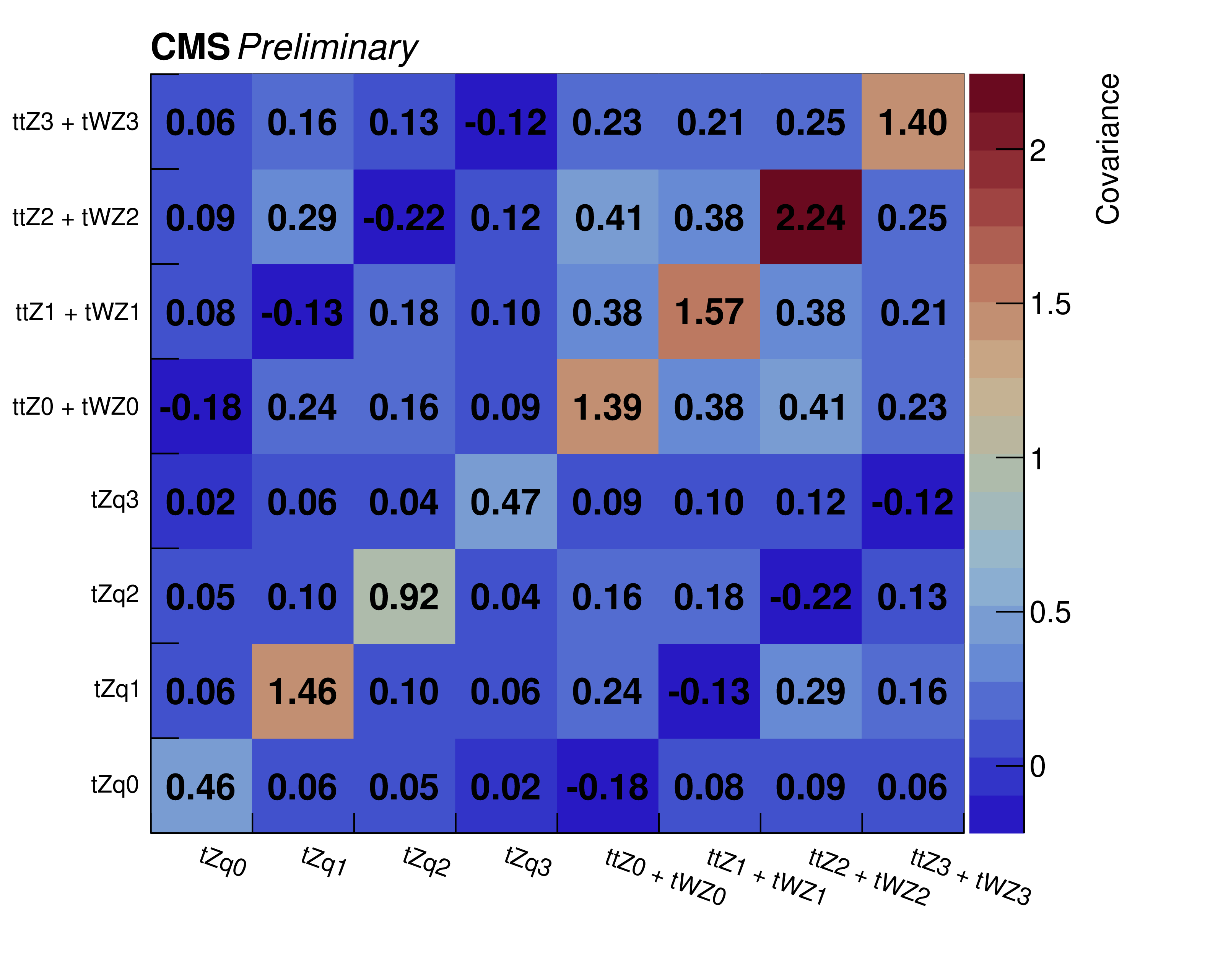
Covariance matrices for the simultaneous fit. The plot refers to the case where the measurement is performed as a function of $ p_{\mathrm{T}}(\mathrm{Z}) $, (upper left), $ p_{\mathrm{T}}(\ell_\mathrm{W}) $ (upper right), $ \Delta R (\mathrm{Z}, \ell_\mathrm{W}) $ (middle left), $ \Delta \phi(\ell^{+},\,\ell^{-}) $ (middle right), and $ \cos\theta^\ast_{\mathrm{Z}} $ (lower). |

png pdf |
Figure 14-a:
Covariance matrices for the simultaneous fit. The plot refers to the case where the measurement is performed as a function of $ p_{\mathrm{T}}(\mathrm{Z}) $, (upper left), $ p_{\mathrm{T}}(\ell_\mathrm{W}) $ (upper right), $ \Delta R (\mathrm{Z}, \ell_\mathrm{W}) $ (middle left), $ \Delta \phi(\ell^{+},\,\ell^{-}) $ (middle right), and $ \cos\theta^\ast_{\mathrm{Z}} $ (lower). |

png pdf |
Figure 14-b:
Covariance matrices for the simultaneous fit. The plot refers to the case where the measurement is performed as a function of $ p_{\mathrm{T}}(\mathrm{Z}) $, (upper left), $ p_{\mathrm{T}}(\ell_\mathrm{W}) $ (upper right), $ \Delta R (\mathrm{Z}, \ell_\mathrm{W}) $ (middle left), $ \Delta \phi(\ell^{+},\,\ell^{-}) $ (middle right), and $ \cos\theta^\ast_{\mathrm{Z}} $ (lower). |
png pdf |
Figure 14-c:
Covariance matrices for the simultaneous fit. The plot refers to the case where the measurement is performed as a function of $ p_{\mathrm{T}}(\mathrm{Z}) $, (upper left), $ p_{\mathrm{T}}(\ell_\mathrm{W}) $ (upper right), $ \Delta R (\mathrm{Z}, \ell_\mathrm{W}) $ (middle left), $ \Delta \phi(\ell^{+},\,\ell^{-}) $ (middle right), and $ \cos\theta^\ast_{\mathrm{Z}} $ (lower). |

png pdf |
Figure 14-d:
Covariance matrices for the simultaneous fit. The plot refers to the case where the measurement is performed as a function of $ p_{\mathrm{T}}(\mathrm{Z}) $, (upper left), $ p_{\mathrm{T}}(\ell_\mathrm{W}) $ (upper right), $ \Delta R (\mathrm{Z}, \ell_\mathrm{W}) $ (middle left), $ \Delta \phi(\ell^{+},\,\ell^{-}) $ (middle right), and $ \cos\theta^\ast_{\mathrm{Z}} $ (lower). |

png pdf |
Figure 14-e:
Covariance matrices for the simultaneous fit. The plot refers to the case where the measurement is performed as a function of $ p_{\mathrm{T}}(\mathrm{Z}) $, (upper left), $ p_{\mathrm{T}}(\ell_\mathrm{W}) $ (upper right), $ \Delta R (\mathrm{Z}, \ell_\mathrm{W}) $ (middle left), $ \Delta \phi(\ell^{+},\,\ell^{-}) $ (middle right), and $ \cos\theta^\ast_{\mathrm{Z}} $ (lower). |
| Tables | |

png pdf |
Table 1:
Systematic uncertainty sources and their relative impact on the inclusive $ {\mathrm{t}\overline{\mathrm{t}}} \mathrm{Z}+\mathrm{t}\mathrm{W}\mathrm{Z} $ and $ \mathrm{t}\mathrm{Z}\mathrm{q} $ cross section measurement. |
| Summary |
| The first simultaneous measurement of single and pair production of top quarks in association with a Z boson is performed. The data were recorded by the CMS experiment at the CERN LHC in proton-proton collisions at a center-of-mass energy of 13 TeV, corresponding to an integrated luminosity of 138 fb$ ^{-1} $. Events with three leptons are selected. The separation between the signals is achieved using a deep neural network classifier with three output nodes for the combined $ {\mathrm{t}\overline{\mathrm{t}}} \mathrm{Z} $ and $ \mathrm{t}\mathrm{W}\mathrm{Z} $ processes, the $ \mathrm{t}\mathrm{Z}\mathrm{q} $ process, and backgrounds. The inclusive cross sections are measured to be $ \sigma({\mathrm{t}\overline{\mathrm{t}}} \mathrm{Z}+\mathrm{t}\mathrm{W}\mathrm{Z}) = $ 1.14 $ \pm $ 0.07 pb for the sum of $ \mathrm{t}\mathrm{W}\mathrm{Z} $ and $ {\mathrm{t}\overline{\mathrm{t}}} \mathrm{Z} $, and $ \sigma(\mathrm{t}\mathrm{Z}\mathrm{q})= $ 0.81 $ \pm $ 0.10 pb for $ \mathrm{t}\mathrm{Z}\mathrm{q} $ production. Both results are evaluated for a dilepton invariant mass within 70 and 110 GeV. The cross sections are measured differentially as functions of several observables. Generally good agreement is found for the $ \mathrm{t}\mathrm{Z}\mathrm{q} $ process, while for $ {\mathrm{t}\overline{\mathrm{t}}} \mathrm{Z} $+$ \mathrm{t}\mathrm{W}\mathrm{Z} $, a clear trend is observed as a function of the transverse momentum $ p_{\mathrm{T}} $ of the lepton originating from the top quark, leading to a significant excess of the data over expectation at low values of $ p_{\mathrm{T}} $. |
| References | ||||
| 1 | ATLAS Collaboration | Measurement of the $ t\overline{t}W $ and $ t\overline{t}Z $ production cross sections in pp collisions at $ \sqrt{s}= $ 8 TeV with the ATLAS detector | JHEP 11 (2015) 172 | 1509.05276 |
| 2 | ATLAS Collaboration | Measurement of the $ t\bar{t}Z $ and $ t\bar{t}W $ production cross sections in multilepton final states using 3.2 fb$ ^{-1} $ of $ pp $ collisions at $ \sqrt{s} = $ 13 TeV with the ATLAS detector | EPJC 77 (2017) 40 | 1609.01599 |
| 3 | ATLAS Collaboration | Measurement of the production cross-section of a single top quark in association with a Z boson in proton-proton collisions at 13 TeV with the ATLAS detector | PLB 780 (2018) 557 | 1710.03659 |
| 4 | ATLAS Collaboration | Measurement of the $ t\bar{t}Z $ and $ t\bar{t}W $ cross sections in proton-proton collisions at $ \sqrt{s}= $ 13 TeV with the ATLAS detector | PRD 99 (2019) 072009 | 1901.03584 |
| 5 | ATLAS Collaboration | Observation of the associated production of a top quark and a Z boson in pp collisions at $ \sqrt{s} = $ 13 TeV with the ATLAS detector | JHEP 07 (2020) 124 | 2002.07546 |
| 6 | ATLAS Collaboration | Measurements of the inclusive and differential production cross sections of a top-quark-antiquark pair in association with a Z boson at $ \sqrt{s} = $ 13 TeV with the ATLAS detector | EPJC 81 (2021) 737 | 2103.12603 |
| 7 | CMS Collaboration | Observation of top quark pairs produced in association with a vector boson in pp collisions at $ \sqrt{s}= $ 8 TeV | JHEP 01 (2016) 096 | CMS-TOP-14-021 1510.01131 |
| 8 | CMS Collaboration | Measurement of the cross section for top quark pair production in association with a W or Z boson in proton-proton collisions at $ \sqrt{s} = $ 13 TeV | JHEP 08 (2018) 011 | CMS-TOP-17-005 1711.02547 |
| 9 | CMS Collaboration | Measurement of the associated production of a single top quark and a Z boson in pp collisions at $ \sqrt{s} = $ 13 TeV | PLB 779 (2018) 358 | CMS-TOP-16-020 1712.02825 |
| 10 | CMS Collaboration | Observation of single top quark production in association with a Z boson in proton-proton collisions at $ \sqrt {s} = $ 13 TeV | PRL 122 (2019) 132003 | CMS-TOP-18-008 1812.05900 |
| 11 | CMS Collaboration | Measurement of top quark pair production in association with a Z boson in proton-proton collisions at $ \sqrt{s}= $ 13 TeV | JHEP 03 (2020) 056 | CMS-TOP-18-009 1907.11270 |
| 12 | CMS Collaboration | Inclusive and differential cross section measurements of single top quark production in association with a Z boson in proton-proton collisions at $ \sqrt{s} = $ 13 TeV | JHEP 02 (2022) 107 | CMS-TOP-20-010 2111.02860 |
| 13 | W. Buchmüller and D. Wyler | Effective lagrangian analysis of new interactions and flavour conservation | Nucl. Phys. B 268 () 621, 1986 Nucl. Phys. B 268 (1996) 621 |
|
| 14 | C. P. Burgess | Introduction to Effective Field Theory | Ann. Rev. Nucl. Part. Sci. 57 (2007) 329 | hep-th/0701053 |
| 15 | SMEFiT Collaboration | Combined SMEFT interpretation of Higgs, diboson, and top quark data from the LHC | JHEP 11 (2021) 089 | 2105.00006 |
| 16 | N. Castro et al. | LHC EFT WG Report: Experimental Measurements and Observables | 2211.08353 | |
| 17 | R. Frederix et al. | The automation of next-to-leading order electroweak calculations | JHEP 07 (2018) 185 | 1804.10017 |
| 18 | D. Pagani, I. Tsinikos, and E. Vryonidou | NLO QCD+EW predictions for $ tHj $ and $ tZj $ production at the LHC | JHEP 08 (2020) 082 | 2006.10086 |
| 19 | CMS Collaboration | Evidence for tWZ production in proton-proton collisions at $ \sqrt{s} = $ 13TeV in multilepton final states | submitted to PLB | CMS-TOP-22-008 2312.11668 |
| 20 | H. E. Faham, F. Maltoni, K. Mimasu, and M. Zaro | Single top production in association with a WZ pair at the LHC in the SMEFT | JHEP 01 (2022) 100 | 2111.03080 |
| 21 | CMS Collaboration | The CMS experiment at the CERN LHC | JINST 3 (2008) S08004 | |
| 22 | CMS Collaboration | Development of the CMS detector for the CERN LHC Run 3 | Accepted by JINST, 2023 | CMS-PRF-21-001 2309.05466 |
| 23 | CMS Collaboration | Particle-flow reconstruction and global event description with the CMS detector | JINST 12 (2017) P10003 | CMS-PRF-14-001 1706.04965 |
| 24 | CMS Collaboration | Technical proposal for the Phase-II upgrade of the Compact Muon Solenoid | CMS Technical Proposal CERN-LHCC-2015-010, CMS-TDR-15-02, 2015 CDS |
|
| 25 | M. Cacciari, G. P. Salam, and G. Soyez | The anti-$ k_t $ jet clustering algorithm | JHEP 04 (2008) 063 | 0802.1189 |
| 26 | M. Cacciari, G. P. Salam, and G. Soyez | FastJet user manual | EPJC 72 (2012) 1896 | 1111.6097 |
| 27 | CMS Collaboration | Identification of heavy-flavour jets with the CMS detector in pp collisions at 13 TeV | JINST 13 (2018) P05011 | CMS-BTV-16-002 1712.07158 |
| 28 | CMS Collaboration | Performance of missing transverse momentum reconstruction in proton-proton collisions at $ \sqrt{s} = $ 13 TeV using the CMS detector | JINST 14 (2019) P07004 | CMS-JME-17-001 1903.06078 |
| 29 | J. Alwall et al. | The automated computation of tree-level and next-to-leading order differential cross sections, and their matching to parton shower simulations | JHEP 07 (2014) 079 | 1405.0301 |
| 30 | S. Frixione, P. Nason, and C. Oleari | Matching NLO QCD computations with parton shower simulations: the POWHEG method | JHEP 11 (2007) 070 | 0709.2092 |
| 31 | J. M. Campbell and R. Ellis | MCFM for the Tevatron and the LHC | Loops and Legs in Quantum Field Theory, 2010 NPB Proc. Supp. 205 (2010) 10 |
|
| 32 | T. Sjöstrand et al. | An introduction to PYTHIA 8.2 | Comput. Phys. Commun. 191 (2015) 159 | 1410.3012 |
| 33 | CMS Collaboration | Extraction and validation of a new set of CMS PYTHIA 8 tunes from underlying-event measurements | EPJC 80 (2020) | CMS-GEN-17-001 1903.12179 |
| 34 | R. Frederix and S. Frixione | Merging meets matching in MC@NLO | JHEP 12 (2012) 061 | 1209.6215 |
| 35 | J. Alwall et al. | Comparative study of various algorithms for the merging of parton showers and matrix elements in hadronic collisions | EPJC 53 (2007) 473 | |
| 36 | NNPDF Collaboration | Parton distributions from high-precision collider data | EPJC 77 (2017) 663 | 1706.00428 |
| 37 | S. Frixione et al. | Single-top hadroproduction in association with a W boson | JHEP 07 (2008) 029 | 0805.3067 |
| 38 | F. Demartin et al. | tWH associated production at the LHC | EPJC 77 (2017) 34 | 1607.05862 |
| 39 | CMS Collaboration | Observation of four top quark production in proton-proton collisions at $ \sqrt{s} = $ 13 TeV | PLB 847 (2023) 138290 | CMS-TOP-22-013 2305.13439 |
| 40 | CMS Collaboration | Electron and photon reconstruction and identification with the CMS experiment at the CERN LHC | JINST 16 (2021) P05014 | CMS-EGM-17-001 2012.06888 |
| 41 | CMS Collaboration | Performance of the CMS muon detector and muon reconstruction with proton-proton collisions at $ \sqrt{s}= $ 13 TeV | JINST 13 (2018) P06015 | CMS-MUO-16-001 1804.04528 |
| 42 | M. Abadi et al. | Tensorflow: large-scale machine learning on heterogeneous systems | Software available from tensorflow.org link |
|
| 43 | Particle Data Group Collaboration | Review of Particle Physics | PTEP 2022 (2022) 083C01 | |
| 44 | CMS Collaboration | Precision luminosity measurement in proton-proton collisions at $ \sqrt{s} = $ 13 TeV in 2015 and 2016 at CMS | EPJC 81 (2021) 800 | CMS-LUM-17-003 2104.01927 |
| 45 | CMS Collaboration | CMS luminosity measurement for the 2017 data-taking period at $ \sqrt{s} = $ 13 TeV | CMS Physics Analysis Summary, 2018 link |
CMS-PAS-LUM-17-004 |
| 46 | CMS Collaboration | CMS luminosity measurement for the 2018 data-taking period at $ \sqrt{s} = $ 13 TeV | CMS Physics Analysis Summary, 2019 link |
CMS-PAS-LUM-18-002 |
| 47 | R. Barlow and C. Beeston | Fitting using finite Monte Carlo samples | Computer Physics Communications 77 (1993) 219 | |
| 48 | CMS Collaboration | Probing effective field theory operators in the associated production of top quarks with a Z boson in multilepton final states at $ \sqrt{s} = $ 13 TeV | JHEP 12 (2021) 083 | CMS-TOP-21-001 2107.13896 |
| 49 | C. Degrande et al. | Single-top associated production with a $ Z $ or $ H $ boson at the LHC: the SMEFT interpretation | JHEP 10 (2018) 005 | 1804.07773 |
| 50 | D. Spitzbart | Search for supersymmetric partners and anomalous couplings of the top quark with the CMS experiment | PhD thesis, TU Wien, Austria, 2019 link |
|
|
|
Compact Muon Solenoid LHC, CERN |
|

|

|

|

|

|