

Compact Muon Solenoid
LHC, CERN
| CMS-EGM-13-001 ; CERN-PH-EP-2015-004 | ||
| Performance of electron reconstruction and selection with the CMS detector in proton-proton collisions at $\sqrt{s}$ = 8 TeV | ||
| CMS Collaboration | ||
| 10 February 2015 | ||
| JINST 10 (2015) P06005 | ||
| Abstract: The performance and strategies used in electron reconstruction and selection at CMS are presented based on data corresponding to an integrated luminosity of 19.7 fb$^{-1}$, collected in proton-proton collisions at $ \sqrt{s} = $ 8 TeV at the CERN LHC. The paper focuses on prompt isolated electrons with transverse momenta ranging from about 5 to a few 100 GeV. A detailed description is given of the algorithms used to cluster energy in the electromagnetic calorimeter and to reconstruct electron trajectories in the tracker. The electron momentum is estimated by combining the energy measurement in the calorimeter with the momentum measurement in the tracker. Benchmark selection criteria are presented, and their performances assessed using Z, $\Upsilon$, and $\mathrm{ J } / \psi$ decays into $\mathrm{ e }^+ \mathrm{ e }^-$ pairs. The spectra of the observables relevant to electron reconstruction and selection as well as their global efficiencies are well reproduced by Monte Carlo simulations. The momentum scale is calibrated with an uncertainty smaller than 0.3%. The momentum resolution for electrons produced in Z boson decays ranges from 1.7 to 4.5%, depending on electron pseudorapidity and energy loss through bremsstrahlung in the detector material. | ||
| Links: e-print arXiv:1502.02701 [physics.ins-det] (PDF) ; CDS record ; inSPIRE record ; CADI line (restricted) ; | ||
| Figures | |

png pdf |
Figure 1:
Two-electron invariant mass spectrum for data collected with dielectron triggers. Electron momenta are obtained by combining information from the tracker and the ECAL. |

png pdf |
Figure 2:
Total thickness of tracker material traversed by a particle produced at the centre of the detector expressed in units of $ {\mathrm {X}_0} $, as a function of particle pseudorapidity $\eta $ in the $ {| \eta | }\leq $ 2.5 acceptance region. The contribution to the total material of each of the subsystems that comprise the CMS tracker is given separately for the pixel tracker, strip tracker consisting of the tracker endcap (TEC), the tracker outer barrel (TOB), the tracker inner barrel (TIB), and the tracker inner disks (TID), together with contributions from the support tube that surrounds the tracker, and from the beam pipe, which is visible as a thin line at the bottom of the figure [5]. |

png pdf |
Figure 3-a:
Comparison of the distributions of the ratio of reconstructed over generated energy for simulated electrons from Z boson decays in a) the barrel, and b) the endcaps, for energies reconstructed using superclustering (solid histogram) and a matrix of 5$\times $5 crystals (dashed histogram). No energy correction is applied to any of the distributions. |
png pdf |
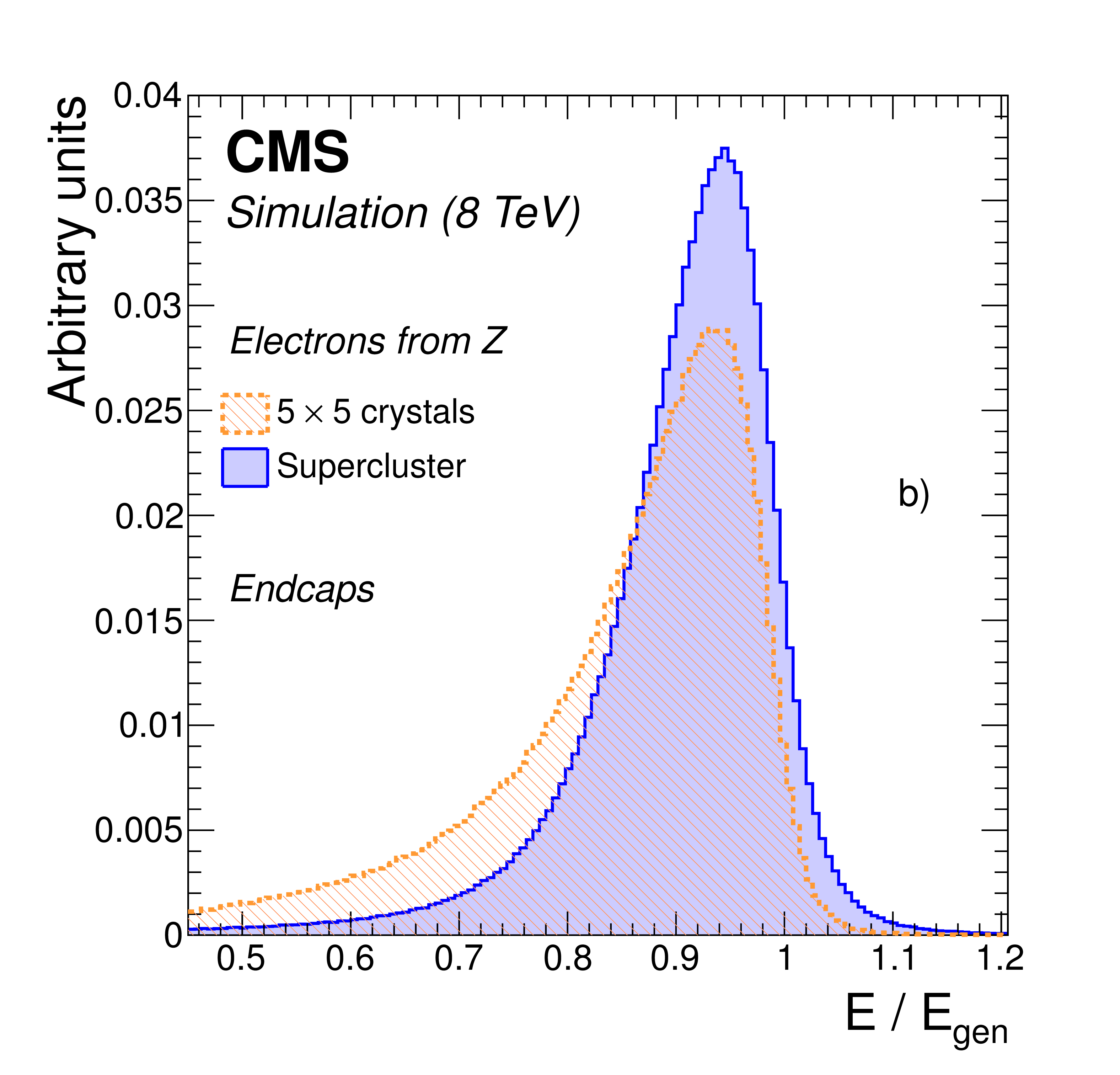
Figure 3-b:
Comparison of the distributions of the ratio of reconstructed over generated energy for simulated electrons from Z boson decays in a) the barrel, and b) the endcaps, for energies reconstructed using superclustering (solid histogram) and a matrix of 5$\times $5 crystals (dashed histogram). No energy correction is applied to any of the distributions. |
png pdf |
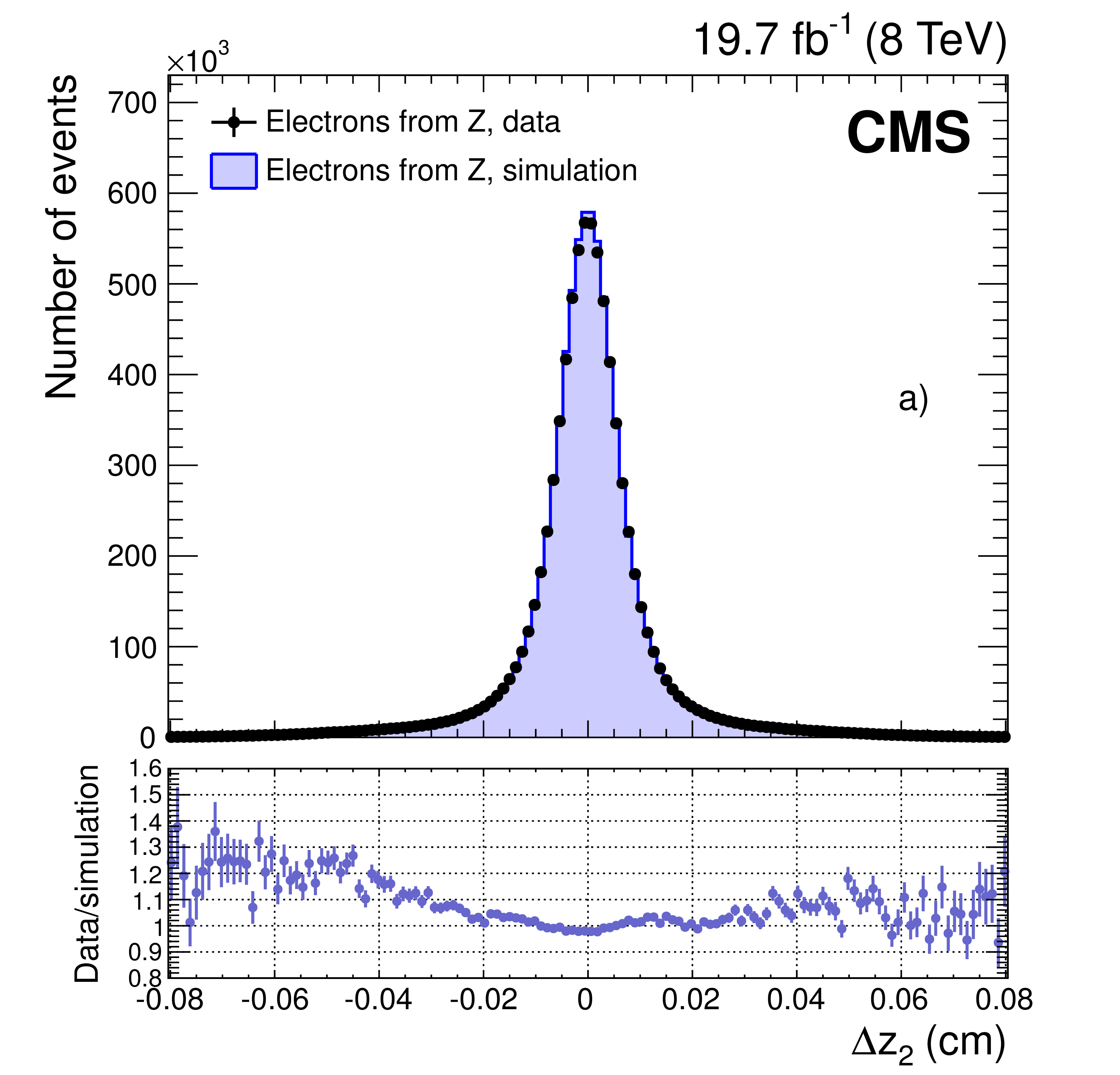
Figure 4-a:
Distributions of the difference between predicted and measured values of the $z_2$ and $\phi _2$ variables for hits in the second window of the ECAL-based seeding, for electrons from ${\mathrm{ Z } } \to \mathrm{ e }^+ \mathrm{ e }^- $ decays in data (dots) and simulation (histograms): a) $\Delta z_2$ (barrel pixel), and b) $\Delta \phi _2$ (all tracker subdetectors). The data-to-simulation ratios are shown below the main panels. |
png pdf |
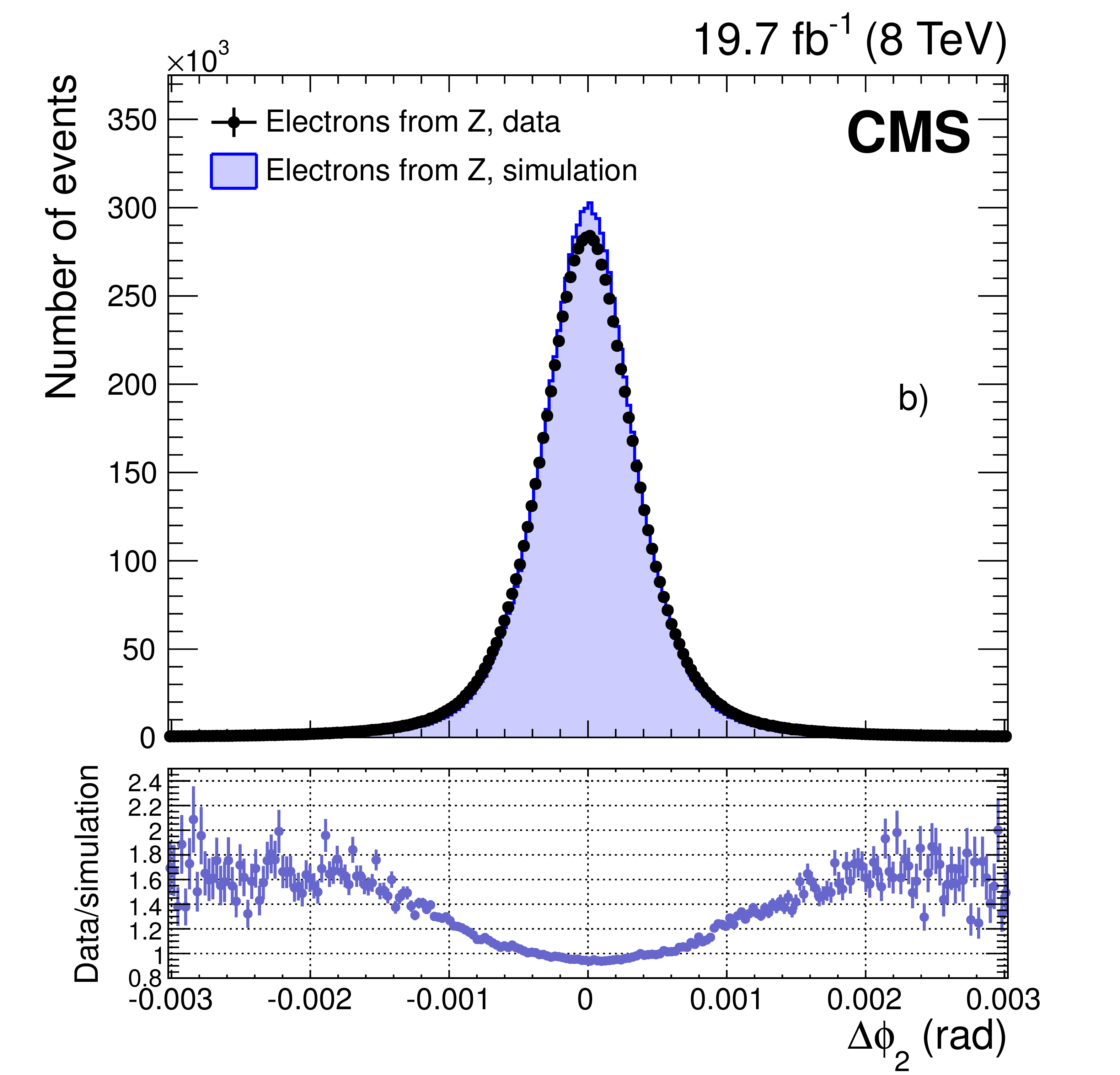
Figure 4-b:
Distributions of the difference between predicted and measured values of the $z_2$ and $\phi _2$ variables for hits in the second window of the ECAL-based seeding, for electrons from ${\mathrm{ Z } } \to \mathrm{ e }^+ \mathrm{ e }^- $ decays in data (dots) and simulation (histograms): a) $\Delta z_2$ (barrel pixel), and b) $\Delta \phi _2$ (all tracker subdetectors). The data-to-simulation ratios are shown below the main panels. |
png pdf |
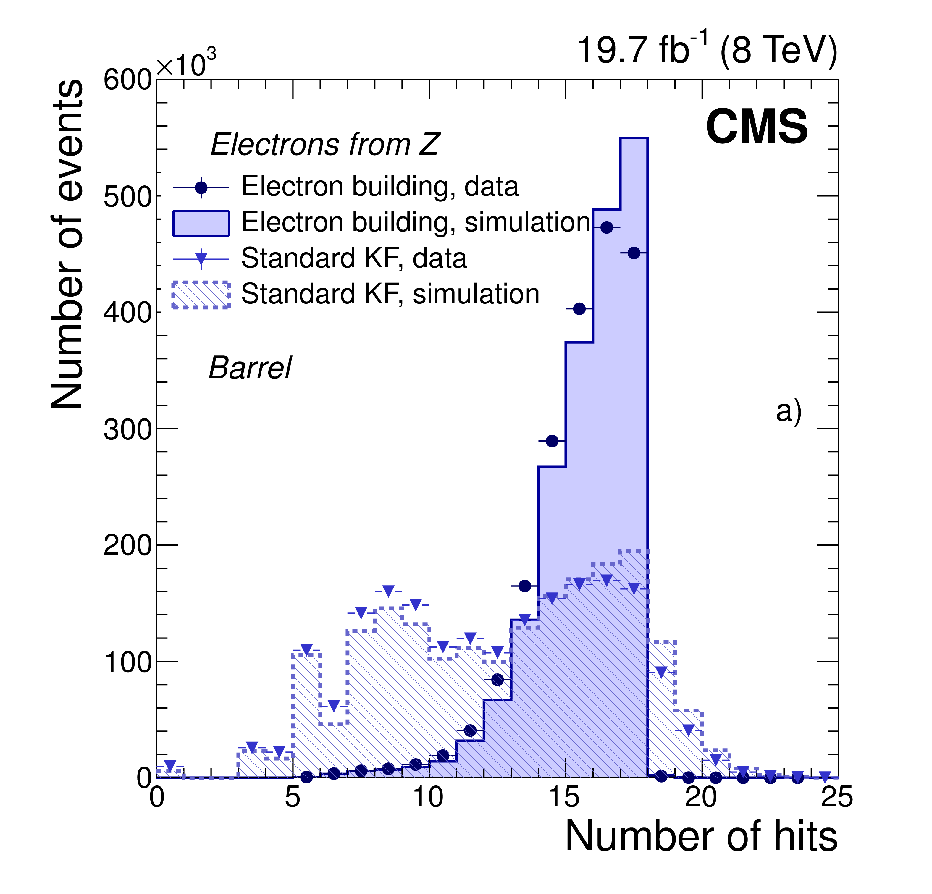
Figure 5-a:
Comparison of the number of hits collected with the dedicated electron building and KF procedures in data (symbols) and in simulation (histograms), for electrons obtained using a ${\mathrm{ Z } } \to \mathrm{ e }^+ \mathrm{ e }^- $ selection, a) in the barrel, and b) in the endcaps. |

png pdf |
Figure 5-b:
Comparison of the number of hits collected with the dedicated electron building and KF procedures in data (symbols) and in simulation (histograms), for electrons obtained using a ${\mathrm{ Z } } \to \mathrm{ e }^+ \mathrm{ e }^- $ selection, a) in the barrel, and b) in the endcaps. |
png pdf |
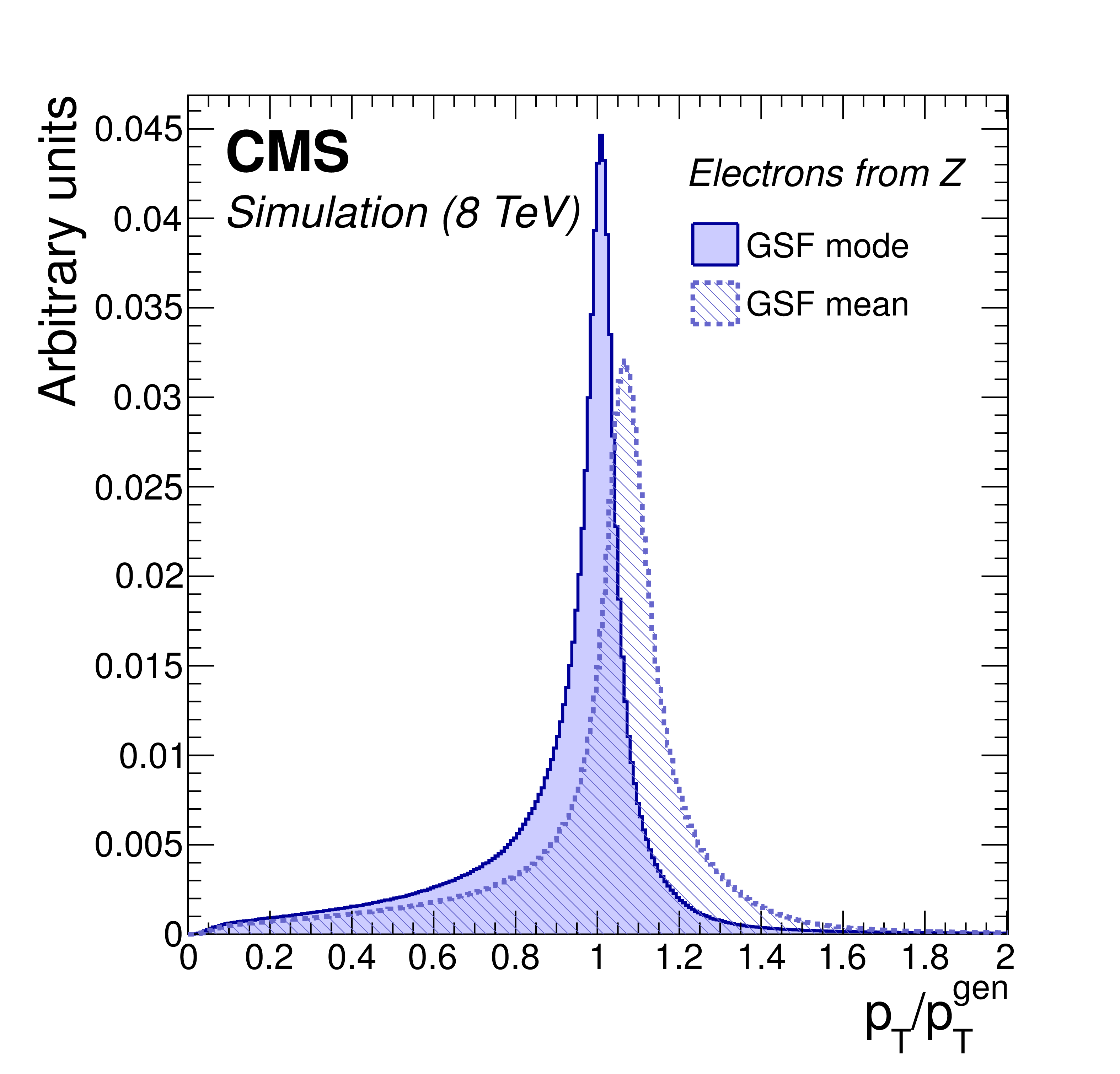
Figure 6:
Distribution of the ratio of reconstructed over generated electron ${p_{\mathrm {T}}}$ in simulated ${\mathrm{ Z } } \to \mathrm{ e }^+ \mathrm{ e }^- $ events, reconstructed through the most probable value of the GSF track components (solid histogram), and its weighted mean (dashed histogram). |
png pdf |
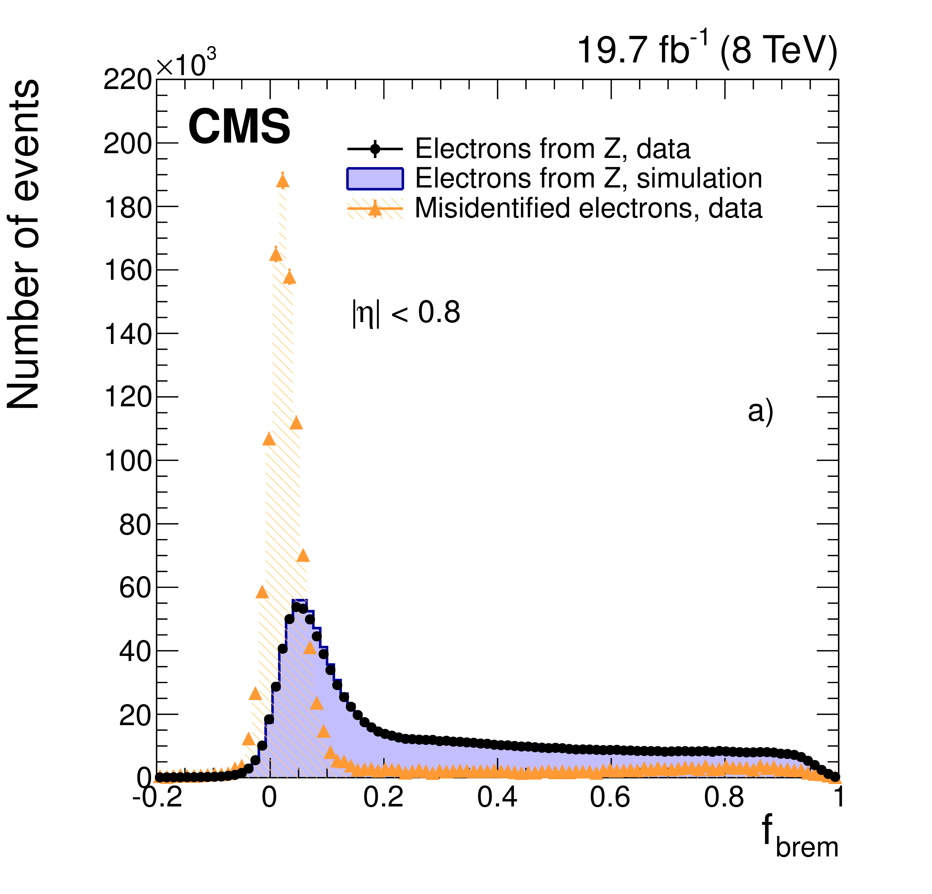
Figure 7-a:
Distribution of $f_{\text {brem}}$ for electrons from ${\mathrm{ Z } } \to \mathrm{ e }^+ \mathrm{ e }^- $ data (dots) and simulated (solid histograms) events, and from background-enriched events in data (triangles), in a) the central barrel $ {| \eta | } <$ 0.8, b) outer barrel 0.8 $< {| \eta | } <$ 1.44, c) endcaps 1.57 $< {| \eta | } <$ 2, and d) endcaps $ {| \eta | } >$ 2. The distributions are normalized to the area of the ${\mathrm{ Z } } \to \mathrm{ e }^+ \mathrm{ e }^- $ data distributions. |
png pdf |
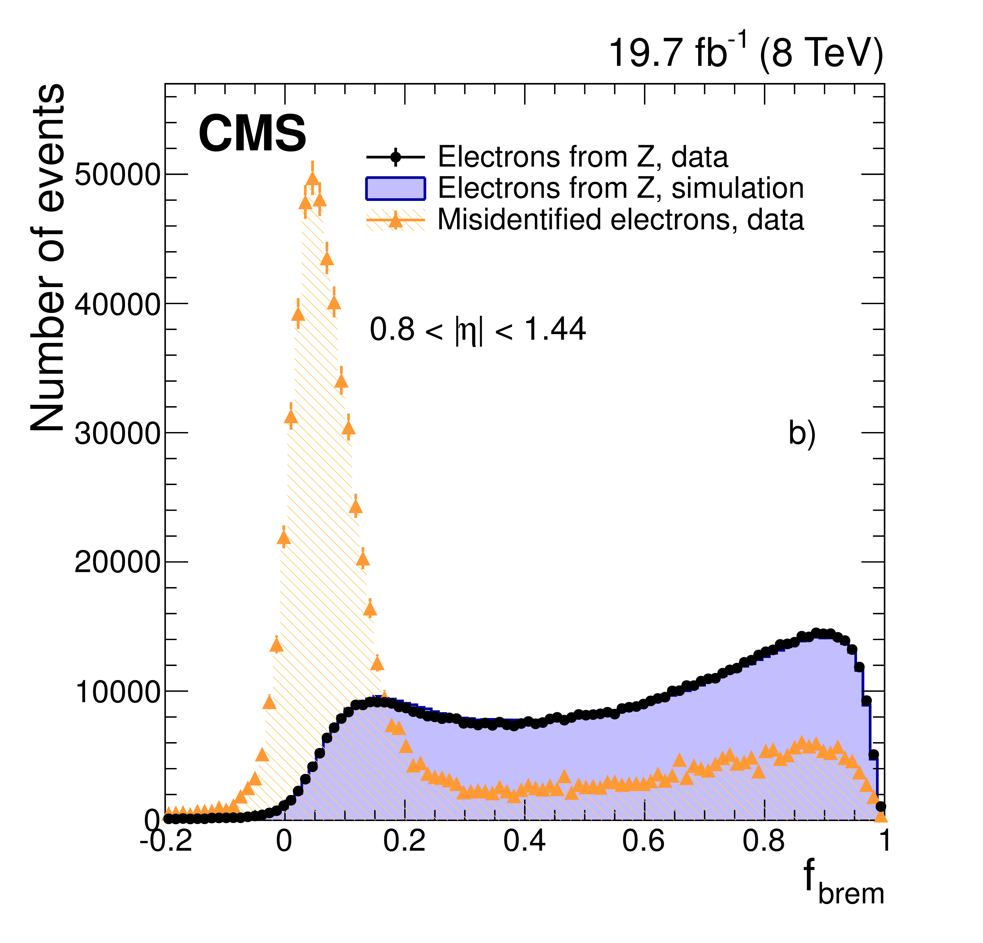
Figure 7-b:
Distribution of $f_{\text {brem}}$ for electrons from ${\mathrm{ Z } } \to \mathrm{ e }^+ \mathrm{ e }^- $ data (dots) and simulated (solid histograms) events, and from background-enriched events in data (triangles), in a) the central barrel $ {| \eta | } <$ 0.8, b) outer barrel 0.8 $< {| \eta | } <$ 1.44, c) endcaps 1.57 $< {| \eta | } <$ 2, and d) endcaps $ {| \eta | } >$ 2. The distributions are normalized to the area of the ${\mathrm{ Z } } \to \mathrm{ e }^+ \mathrm{ e }^- $ data distributions. |
png pdf |
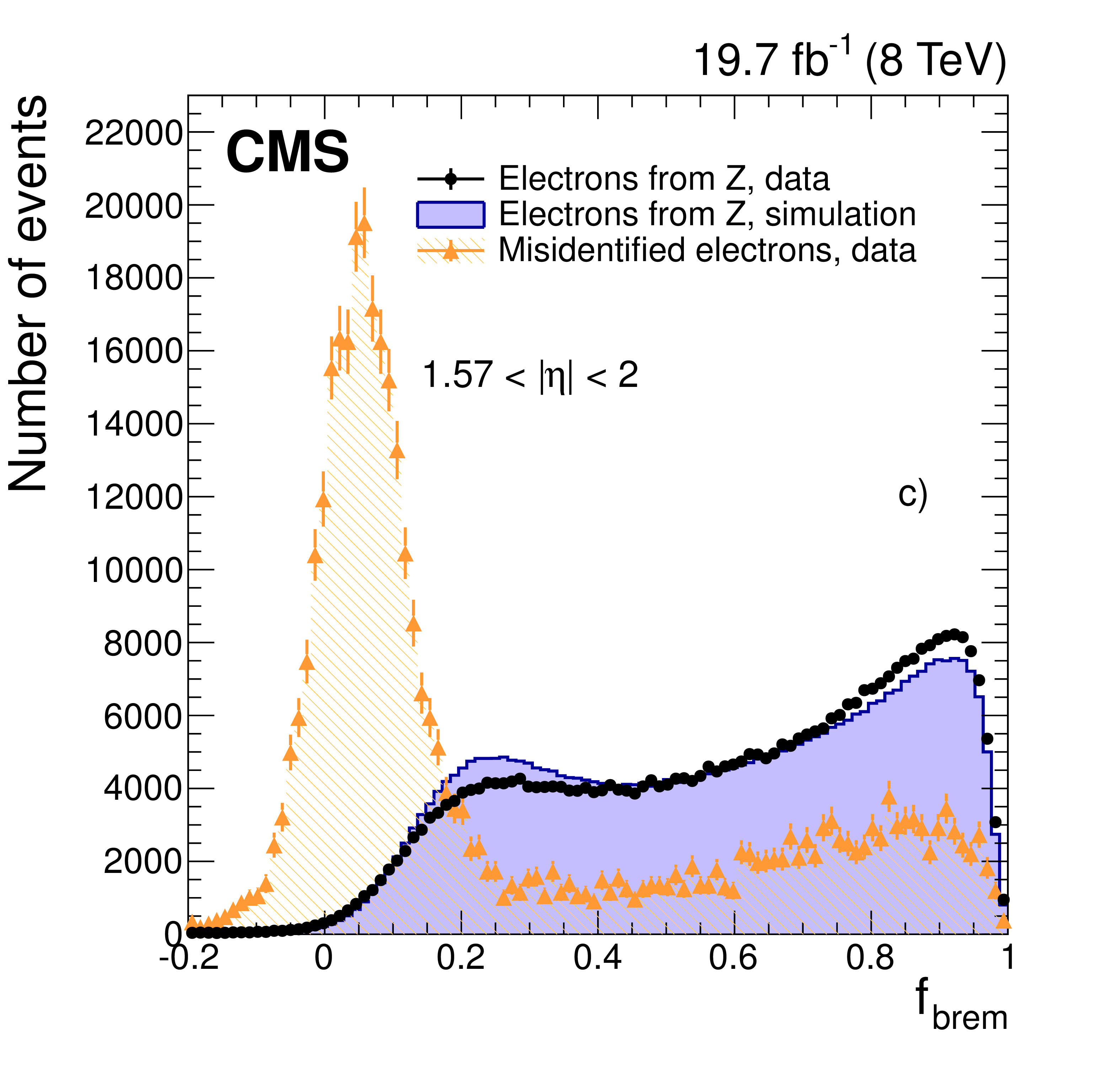
Figure 7-c:
Distribution of $f_{\text {brem}}$ for electrons from ${\mathrm{ Z } } \to \mathrm{ e }^+ \mathrm{ e }^- $ data (dots) and simulated (solid histograms) events, and from background-enriched events in data (triangles), in a) the central barrel $ {| \eta | } <$ 0.8, b) outer barrel 0.8 $< {| \eta | } <$ 1.44, c) endcaps 1.57 $< {| \eta | } <$ 2, and d) endcaps $ {| \eta | } >$ 2. The distributions are normalized to the area of the ${\mathrm{ Z } } \to \mathrm{ e }^+ \mathrm{ e }^- $ data distributions. |
png pdf |
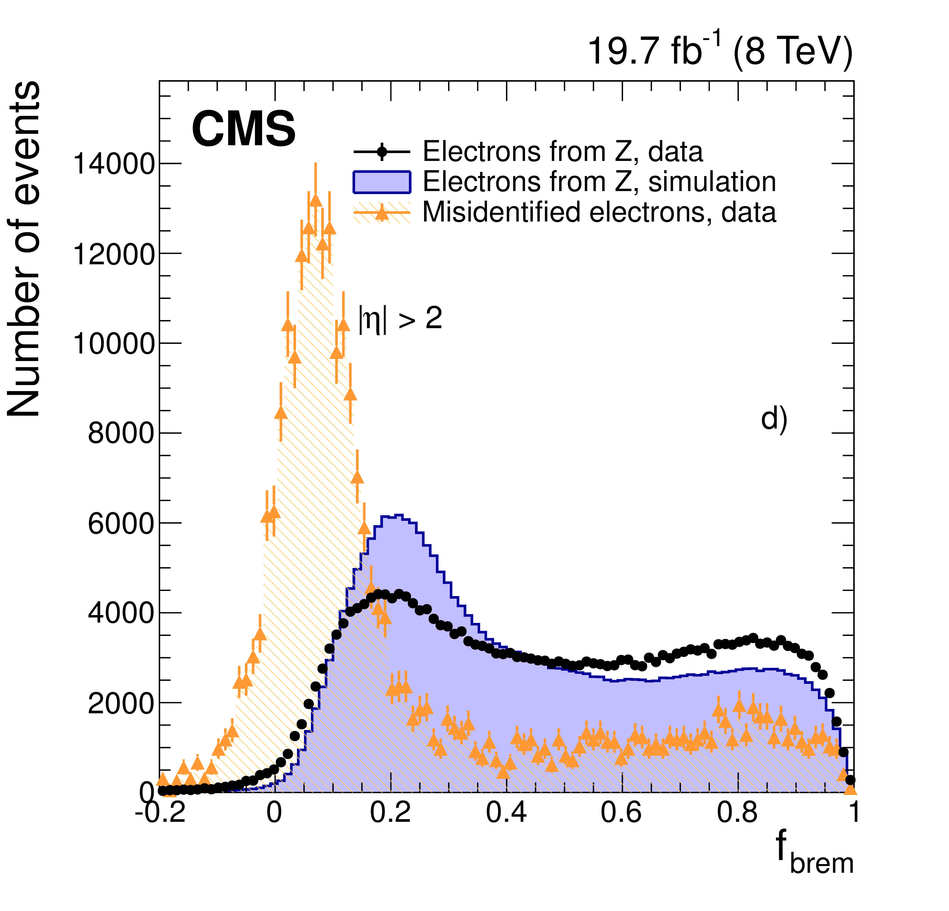
Figure 7-d:
Distribution of $f_{\text {brem}}$ for electrons from ${\mathrm{ Z } } \to \mathrm{ e }^+ \mathrm{ e }^- $ data (dots) and simulated (solid histograms) events, and from background-enriched events in data (triangles), in a) the central barrel $ {| \eta | } <$ 0.8, b) outer barrel 0.8 $< {| \eta | } <$ 1.44, c) endcaps 1.57 $< {| \eta | } <$ 2, and d) endcaps $ {| \eta | } >$ 2. The distributions are normalized to the area of the ${\mathrm{ Z } } \to \mathrm{ e }^+ \mathrm{ e }^- $ data distributions. |

png pdf |
Figure 8-a:
a) Fraction of population in different classes of electrons from Z boson decays as a function of $ {| \eta | }$, for data (dots) and simulated (histograms) events, and b) distribution of $E_{\mathrm {SC}}/E_{\text {gen}}$ for the different classes of simulated electrons. Crack electrons are not shown in either plot. |
png pdf |
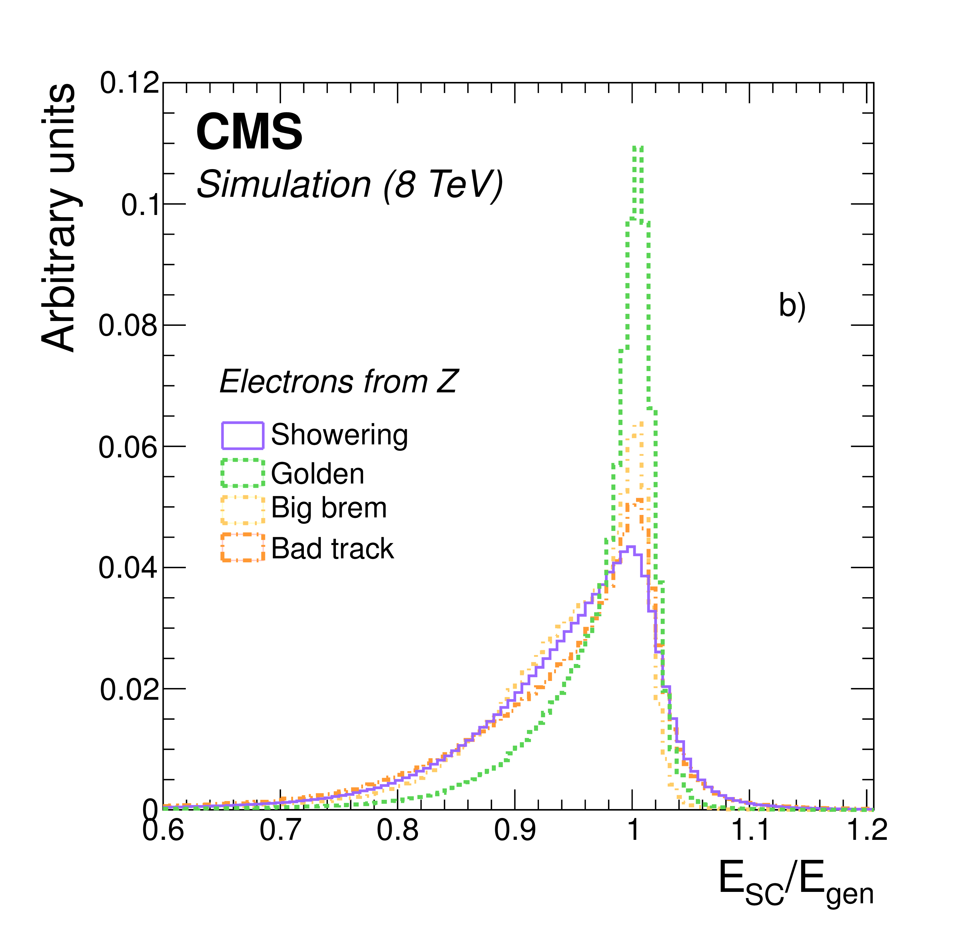
Figure 8-b:
a) Fraction of population in different classes of electrons from Z boson decays as a function of $ {| \eta | }$, for data (dots) and simulated (histograms) events, and b) distribution of $E_{\mathrm {SC}}/E_{\text {gen}}$ for the different classes of simulated electrons. Crack electrons are not shown in either plot. |

png pdf |
Figure 9-a:
Example distributions of the ratio of corrected over generated supercluster energies ($E_{\mathrm {SC}}^{\text {cor}} / E_{\text {gen}}$) and their (double Crystal Ball) fits, in two regions of $\eta $ and ${p_{\mathrm {T}}}$ after implementing the regression corrections: for electrons a) with 7 $\leq {p_{\mathrm {T}}} ^{\text {gen}} < $ 10 GeV and $ {| \eta _{\mathrm {SC}} | } <$ 1, and b) with 30 $\leq {p_{\mathrm {T}}} ^{\text {gen}} < $ 35 GeV and 2 $\leq {| \eta _{\mathrm {SC}} | } <$ 2.5, $\eta _{\mathrm {SC}}$ being defined relative to the centre of CMS. Electrons are generated with uniform distributions in $\eta $ and ${p_{\mathrm {T}}}$ . |
png pdf |
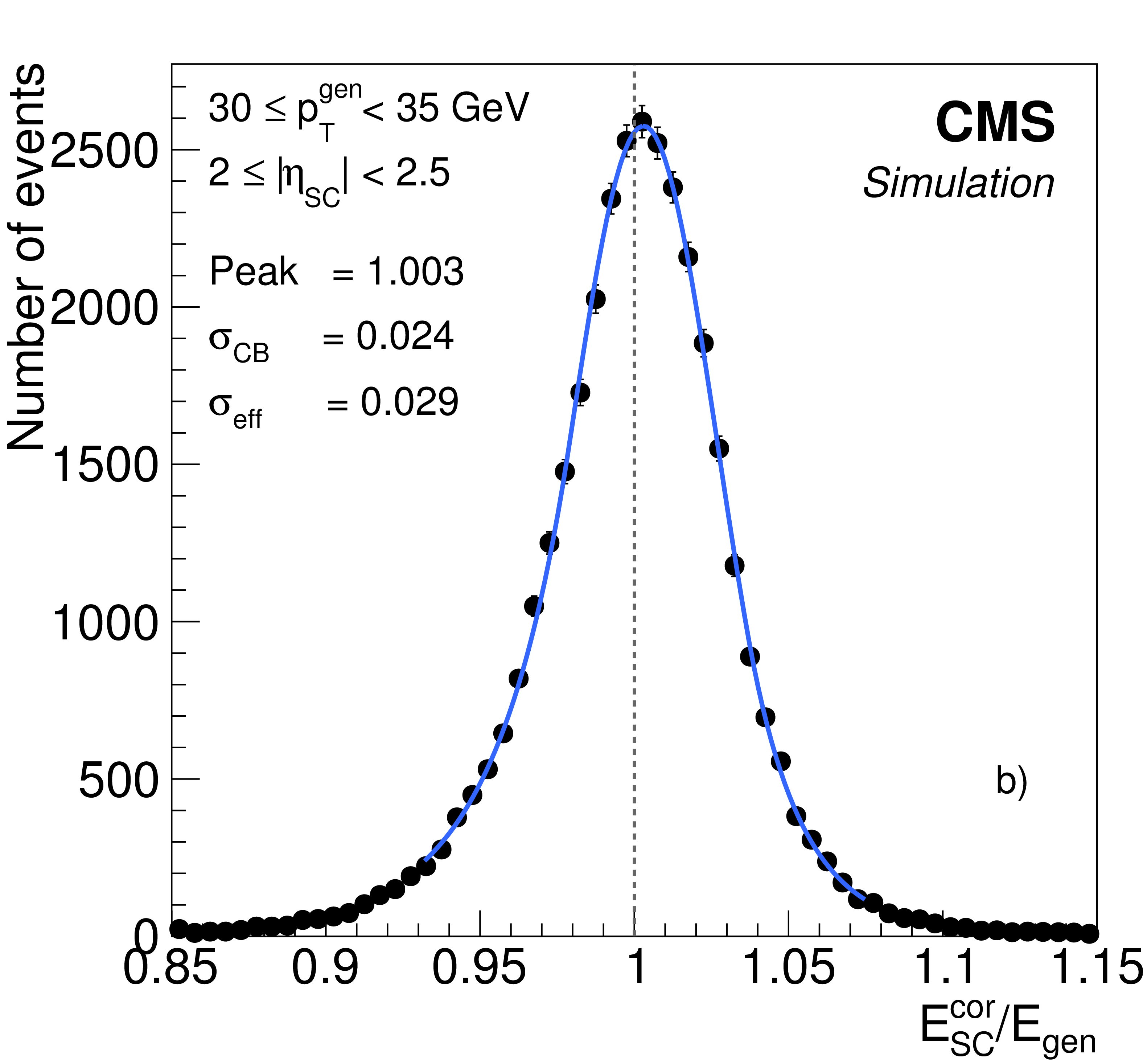
Figure 9-b:
Example distributions of the ratio of corrected over generated supercluster energies ($E_{\mathrm {SC}}^{\text {cor}} / E_{\text {gen}}$) and their (double Crystal Ball) fits, in two regions of $\eta $ and ${p_{\mathrm {T}}}$ after implementing the regression corrections: for electrons a) with 7 $\leq {p_{\mathrm {T}}} ^{\text {gen}} < $ 10 GeV and $ {| \eta _{\mathrm {SC}} | } <$ 1, and b) with 30 $\leq {p_{\mathrm {T}}} ^{\text {gen}} < $ 35 GeV and 2 $\leq {| \eta _{\mathrm {SC}} | } <$ 2.5, $\eta _{\mathrm {SC}}$ being defined relative to the centre of CMS. Electrons are generated with uniform distributions in $\eta $ and ${p_{\mathrm {T}}}$ . |
png pdf |
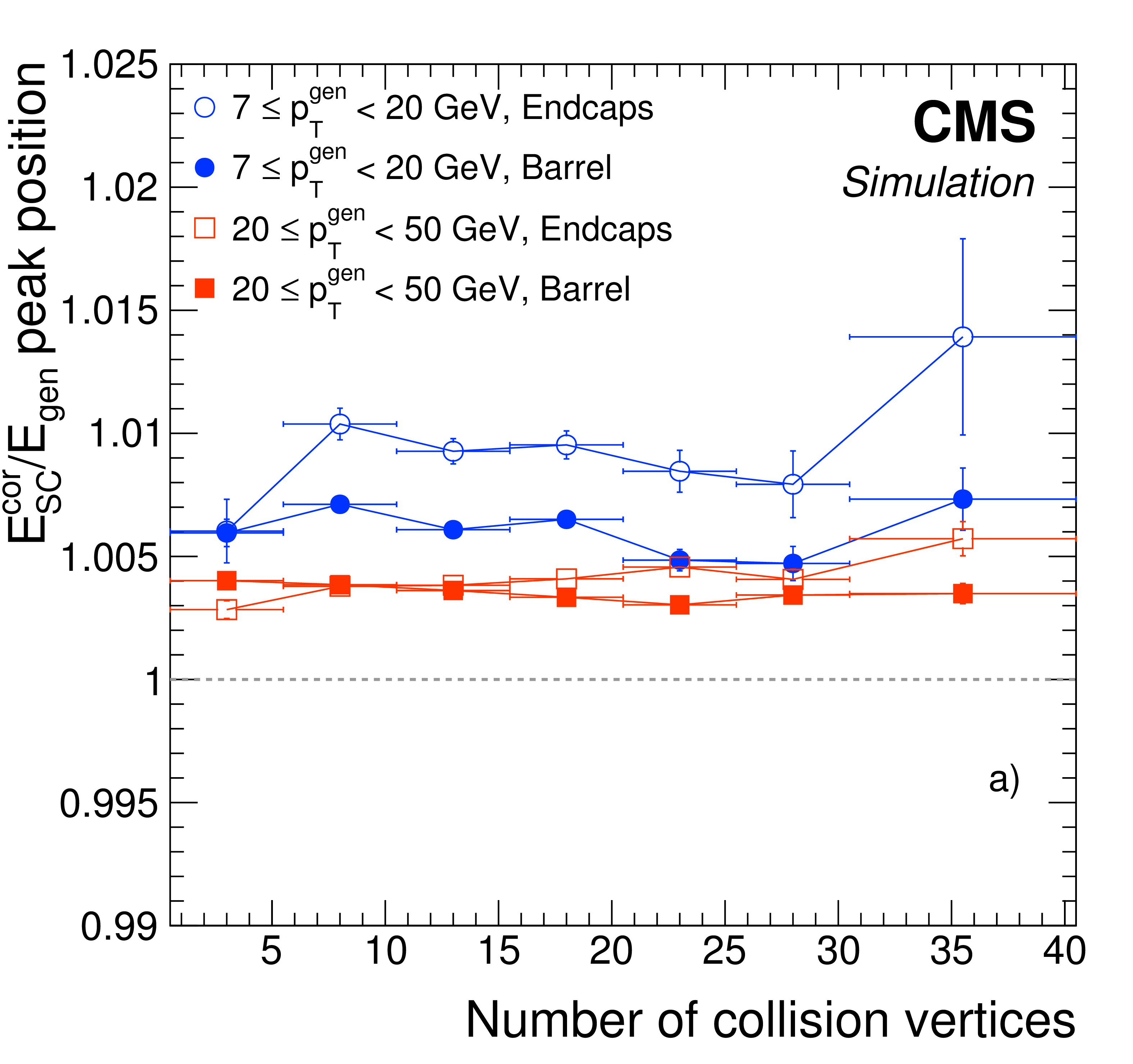
Figure 10-a:
a) Peak position of $E_{\mathrm {SC}}^{\text {cor}} / E_{\text {gen}}$, and b) effective resolution of $E_{\mathrm {SC}}^{\text {cor}}$, as a function of the number of reconstructed interaction vertices, for electrons in the barrel (solid symbols) and endcaps (open symbols) with 7 $\leq {p_{\mathrm {T}}} ^{\text {gen}} < $ 20 GeV (circles), and 20 $\leq {p_{\mathrm {T}}} ^{\text {gen}} <$ 50 GeV (squares). Electrons are generated with uniform distributions in $\eta $ and ${p_{\mathrm {T}}}$ . |
png pdf |
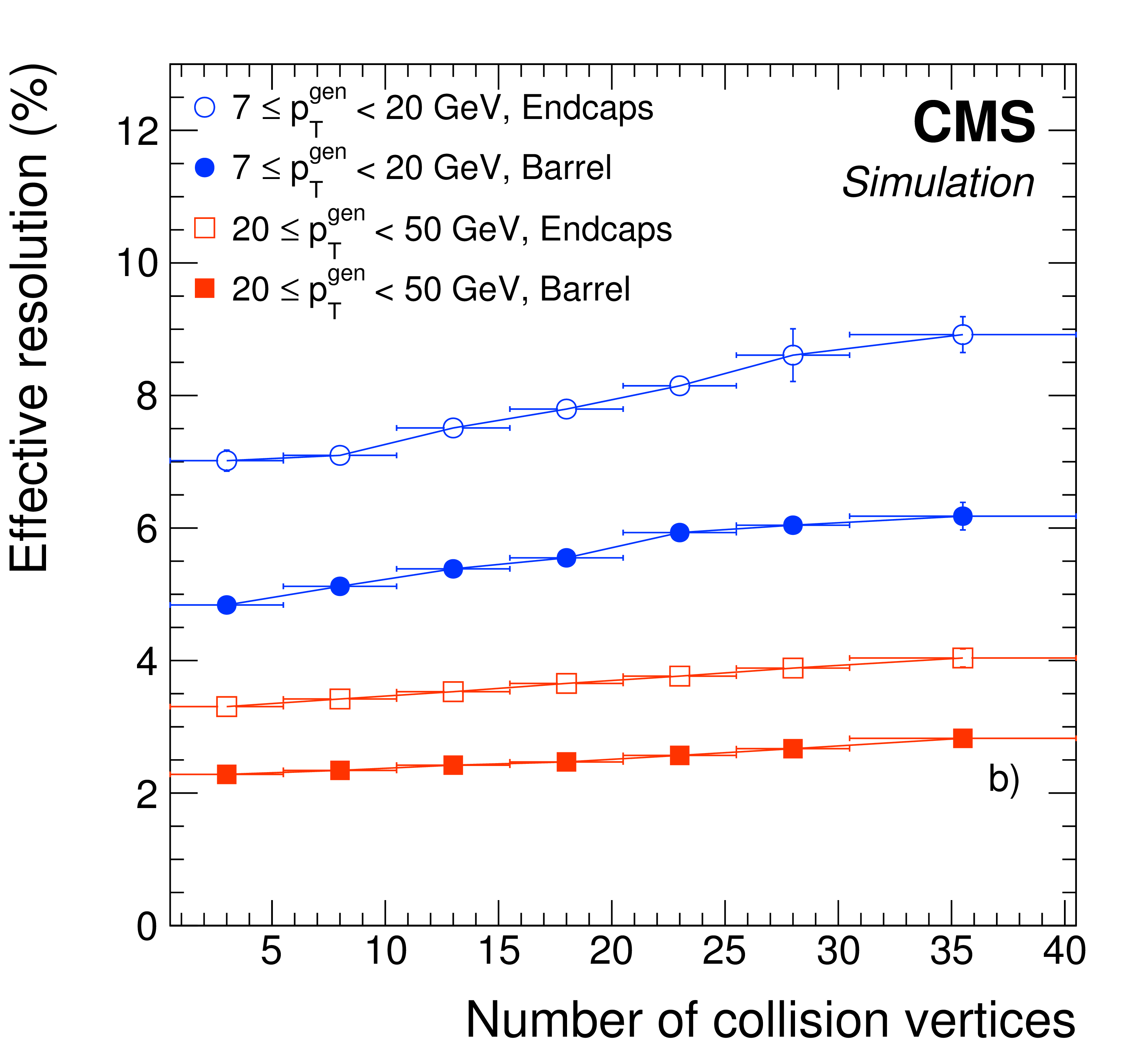
Figure 10-b:
a) Peak position of $E_{\mathrm {SC}}^{\text {cor}} / E_{\text {gen}}$, and b) effective resolution of $E_{\mathrm {SC}}^{\text {cor}}$, as a function of the number of reconstructed interaction vertices, for electrons in the barrel (solid symbols) and endcaps (open symbols) with 7 $\leq {p_{\mathrm {T}}} ^{\text {gen}} < $ 20 GeV (circles), and 20 $\leq {p_{\mathrm {T}}} ^{\text {gen}} <$ 50 GeV (squares). Electrons are generated with uniform distributions in $\eta $ and ${p_{\mathrm {T}}}$ . |
png pdf |
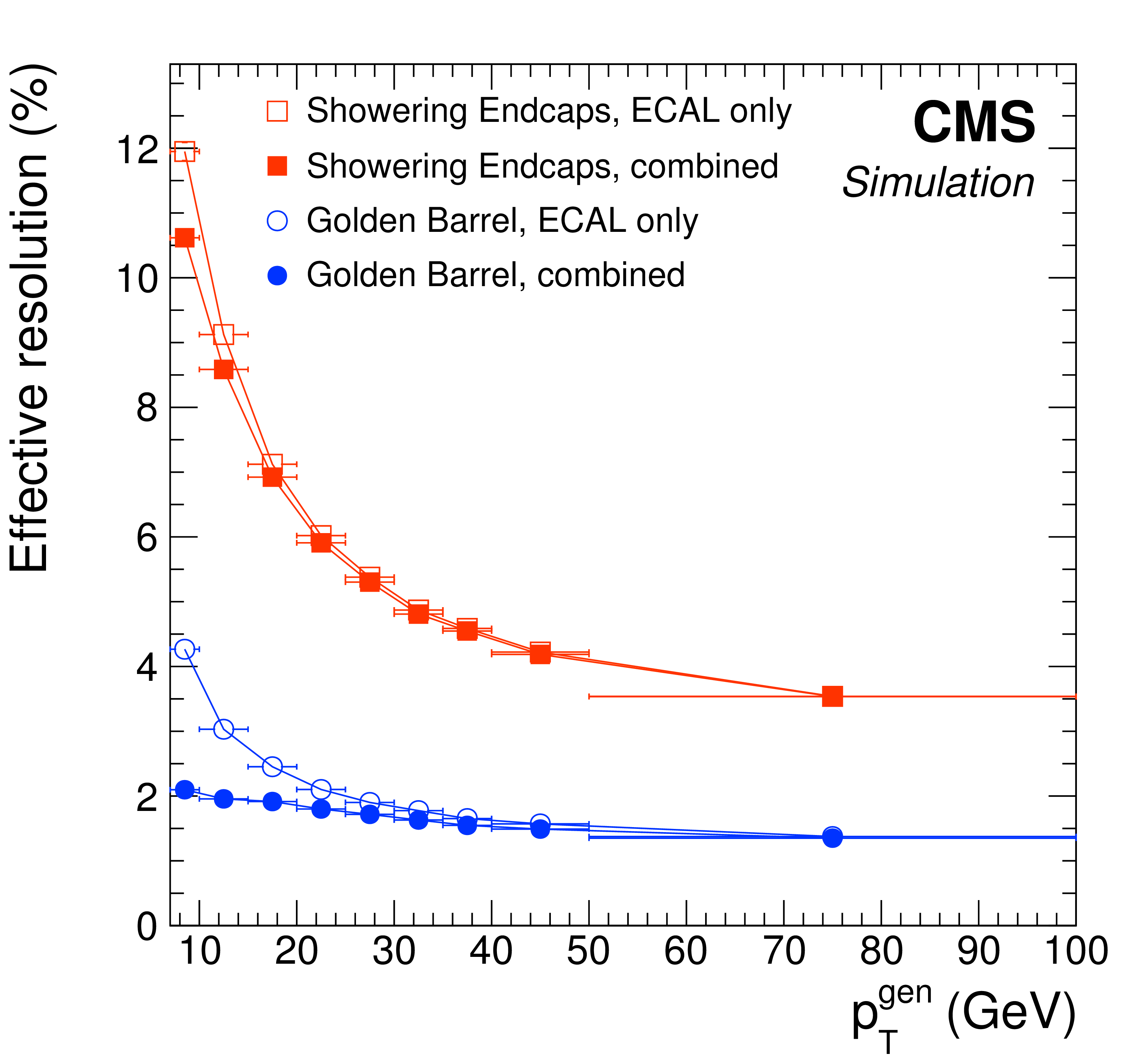
Figure 11:
Effective resolution in electron momentum after combining the $E_{\mathrm {SC}}$ and $p$ estimates (solid symbols), compared to that of the corrected SC energy (open symbols), as a function of the generated electron ${p_{\mathrm {T}}} $. Golden electrons in the barrel (circles) and showering electrons in the endcaps (squares) are shown as examples. Electrons are generated with uniform distributions in $\eta $ and ${p_{\mathrm {T}}}$ , and the resolution is shown after applying the resolution broadening. |
png pdf |
Figure 12-a:
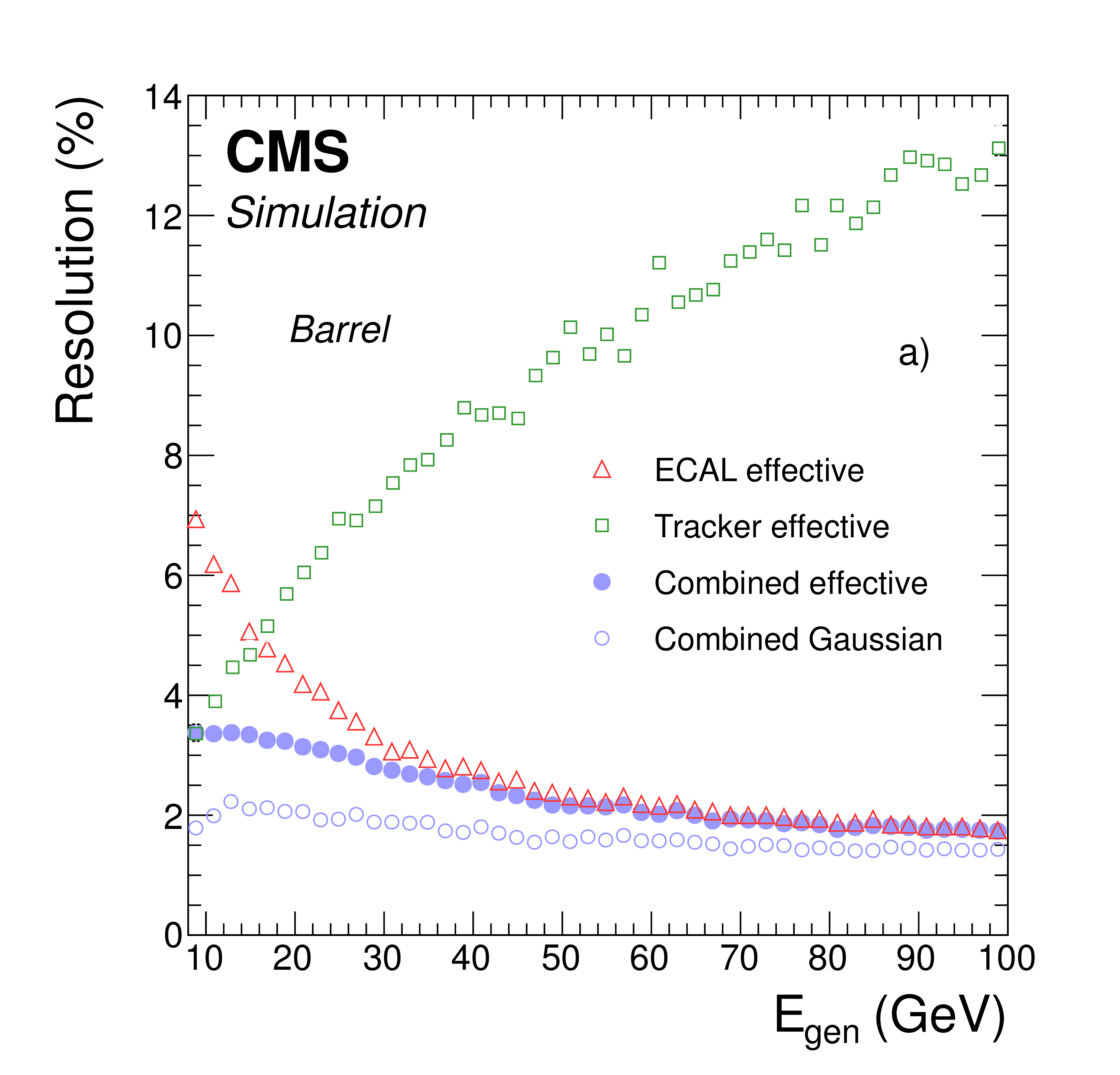
a) Effective resolution in electron momentum after combining $E_{\mathrm {SC}}$ and $p$ estimates (solid circles), compared to those using the corrected SC energy (triangles), and the track momentum (squares), as a function of the generated energy for electrons in the barrel. Also shown is the resolution in momentum after combining $E_{\mathrm {SC}}$ and $p$ estimates in terms of $\sigma _{\mathrm {CB}}$ (open circles), to illustrate the contribution of the Gaussian core of the distribution. Electrons are generated with uniform distributions in $\eta $ and ${p_{\mathrm {T}}} $. b) Reconstructed mass of the Higgs boson for $\mathrm{ H } (126) \to \mathrm{ Z } {\mathrm{ Z } } ^* \to 4\mathrm{ e } $ simulated events, using either the corrected SC energy (open triangles) or the electron momentum after combining $E_{\mathrm {SC}}$ and $p$ estimates (solid dots) [9]. |

png pdf |
Figure 12-b:
a) Effective resolution in electron momentum after combining $E_{\mathrm {SC}}$ and $p$ estimates (solid circles), compared to those using the corrected SC energy (triangles), and the track momentum (squares), as a function of the generated energy for electrons in the barrel. Also shown is the resolution in momentum after combining $E_{\mathrm {SC}}$ and $p$ estimates in terms of $\sigma _{\mathrm {CB}}$ (open circles), to illustrate the contribution of the Gaussian core of the distribution. Electrons are generated with uniform distributions in $\eta $ and ${p_{\mathrm {T}}} $. b) Reconstructed mass of the Higgs boson for $\mathrm{ H } (126) \to \mathrm{ Z } {\mathrm{ Z } } ^* \to 4\mathrm{ e } $ simulated events, using either the corrected SC energy (open triangles) or the electron momentum after combining $E_{\mathrm {SC}}$ and $p$ estimates (solid dots) [9]. |

png pdf |
Figure 13-a:
Dielectron invariant mass distribution from ${\mathrm{ Z } } \to \mathrm{ e }^+ \mathrm{ e }^- $ events in data (solid squares) compared to simulation (open circles) fitted with a convolution of a Breit-Wigner function and a Crystal Ball function, a) for the best-resolved event category with two well-measured single-cluster electrons in the barrel (BGBG), and b) for the worst-resolved category with two more-difficult patterns or multi-cluster electrons in the endcaps (ESES). The masses at which the fitting functions have their maximum values, termed $m_{\text {peak}}$, and the effective standard deviations $\sigma _{\text {eff}}$ are given in the plots. The data-to-simulation factors are shown below the main panels. |
png pdf |
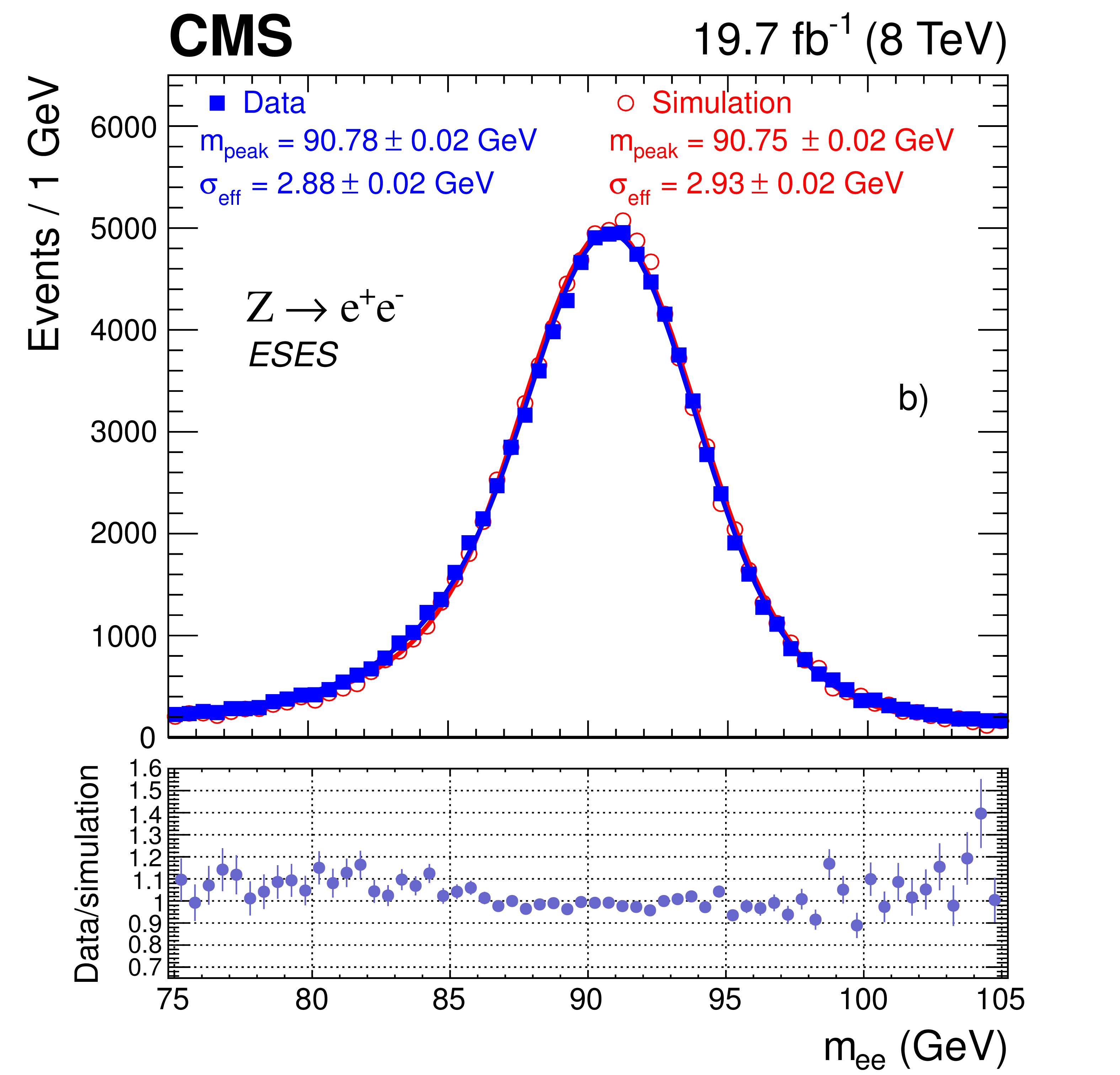
Figure 13-b:
Dielectron invariant mass distribution from ${\mathrm{ Z } } \to \mathrm{ e }^+ \mathrm{ e }^- $ events in data (solid squares) compared to simulation (open circles) fitted with a convolution of a Breit-Wigner function and a Crystal Ball function, a) for the best-resolved event category with two well-measured single-cluster electrons in the barrel (BGBG), and b) for the worst-resolved category with two more-difficult patterns or multi-cluster electrons in the endcaps (ESES). The masses at which the fitting functions have their maximum values, termed $m_{\text {peak}}$, and the effective standard deviations $\sigma _{\text {eff}}$ are given in the plots. The data-to-simulation factors are shown below the main panels. |
png pdf |
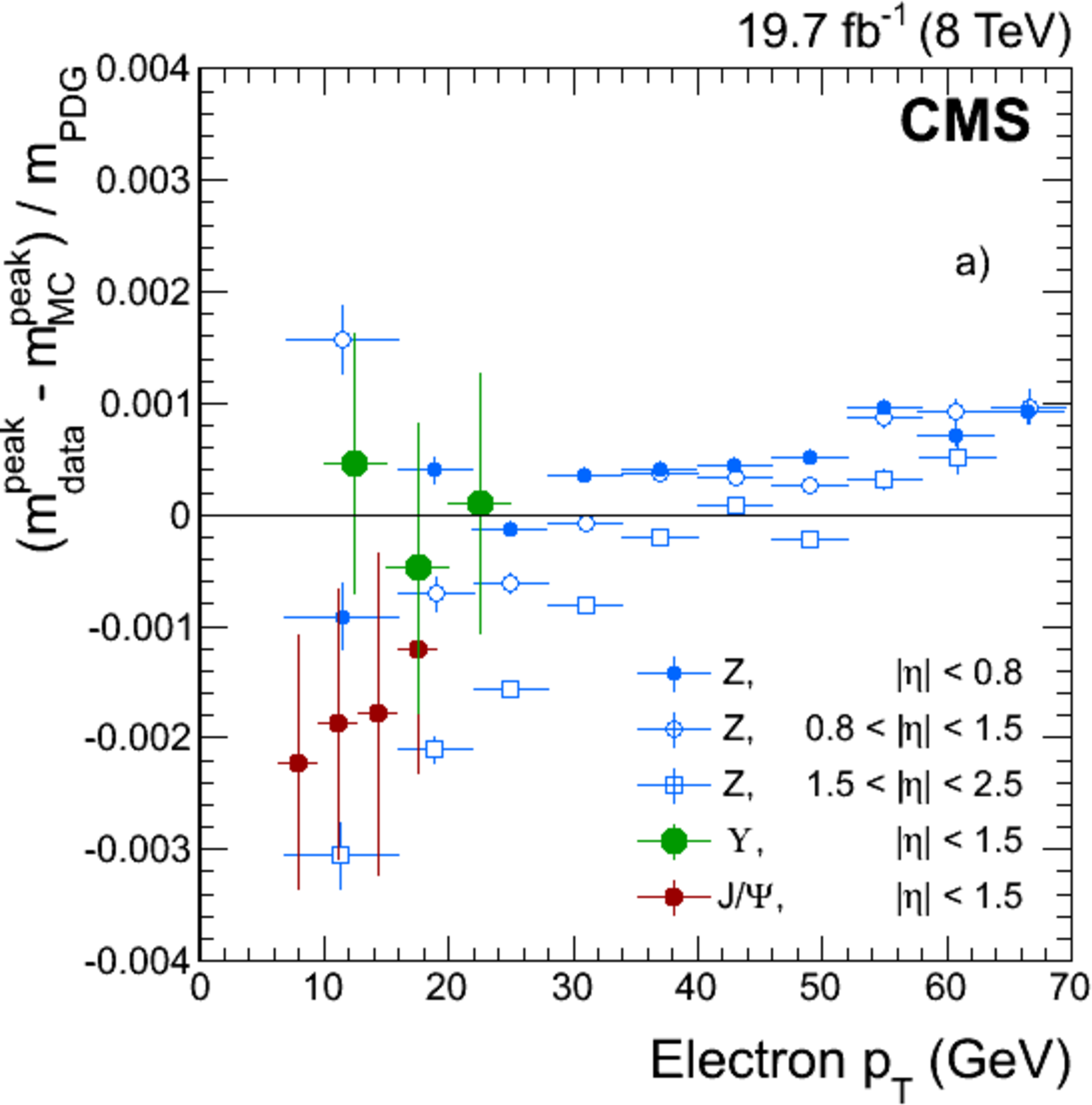
Figure 14-a:
Relative differences between data and simulation as a function of electron ${p_{\mathrm {T}}}$ for different $ {| \eta | }$ regions, a) for the momentum scale measured using ${\mathrm{ J } / \psi } \to \mathrm{ e }^+ \mathrm{ e }^- $, $\Upsilon \to \mathrm{ e }^+ \mathrm{ e }^- $, and ${\mathrm{ Z } } \to \mathrm{ e }^+ \mathrm{ e }^- $ events [9], and b) for the effective momentum resolution of ${\mathrm{ Z } } \to \mathrm{ e }^+ \mathrm{ e }^- $ and ${\mathrm{ J } / \psi } \to \mathrm{ e }^+ \mathrm{ e }^- $ events for different electron categories. |
png pdf |
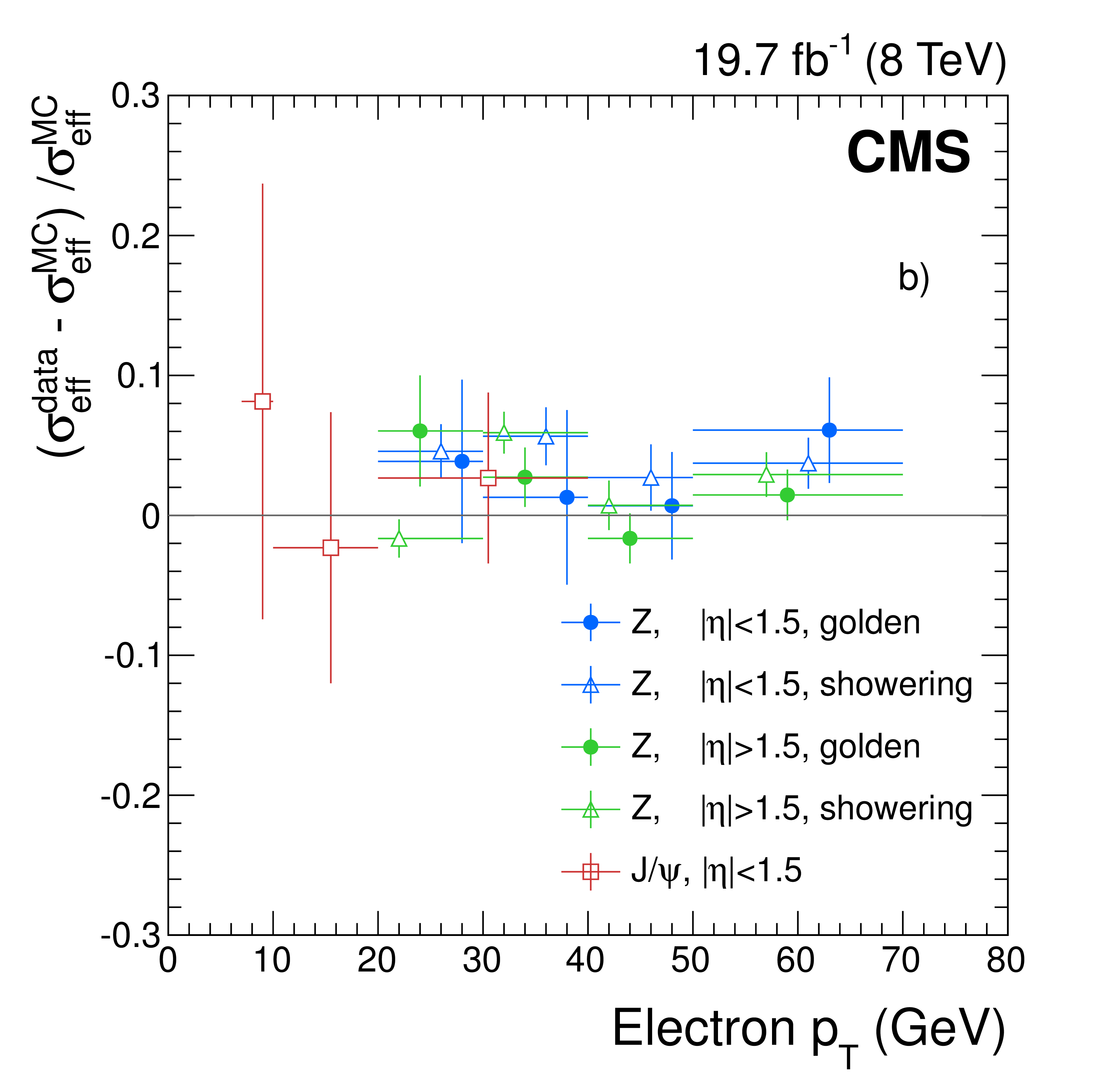
Figure 14-b:
Relative differences between data and simulation as a function of electron ${p_{\mathrm {T}}}$ for different $ {| \eta | }$ regions, a) for the momentum scale measured using ${\mathrm{ J } / \psi } \to \mathrm{ e }^+ \mathrm{ e }^- $, $\Upsilon \to \mathrm{ e }^+ \mathrm{ e }^- $, and ${\mathrm{ Z } } \to \mathrm{ e }^+ \mathrm{ e }^- $ events [9], and b) for the effective momentum resolution of ${\mathrm{ Z } } \to \mathrm{ e }^+ \mathrm{ e }^- $ and ${\mathrm{ J } / \psi } \to \mathrm{ e }^+ \mathrm{ e }^- $ events for different electron categories. |
png pdf |
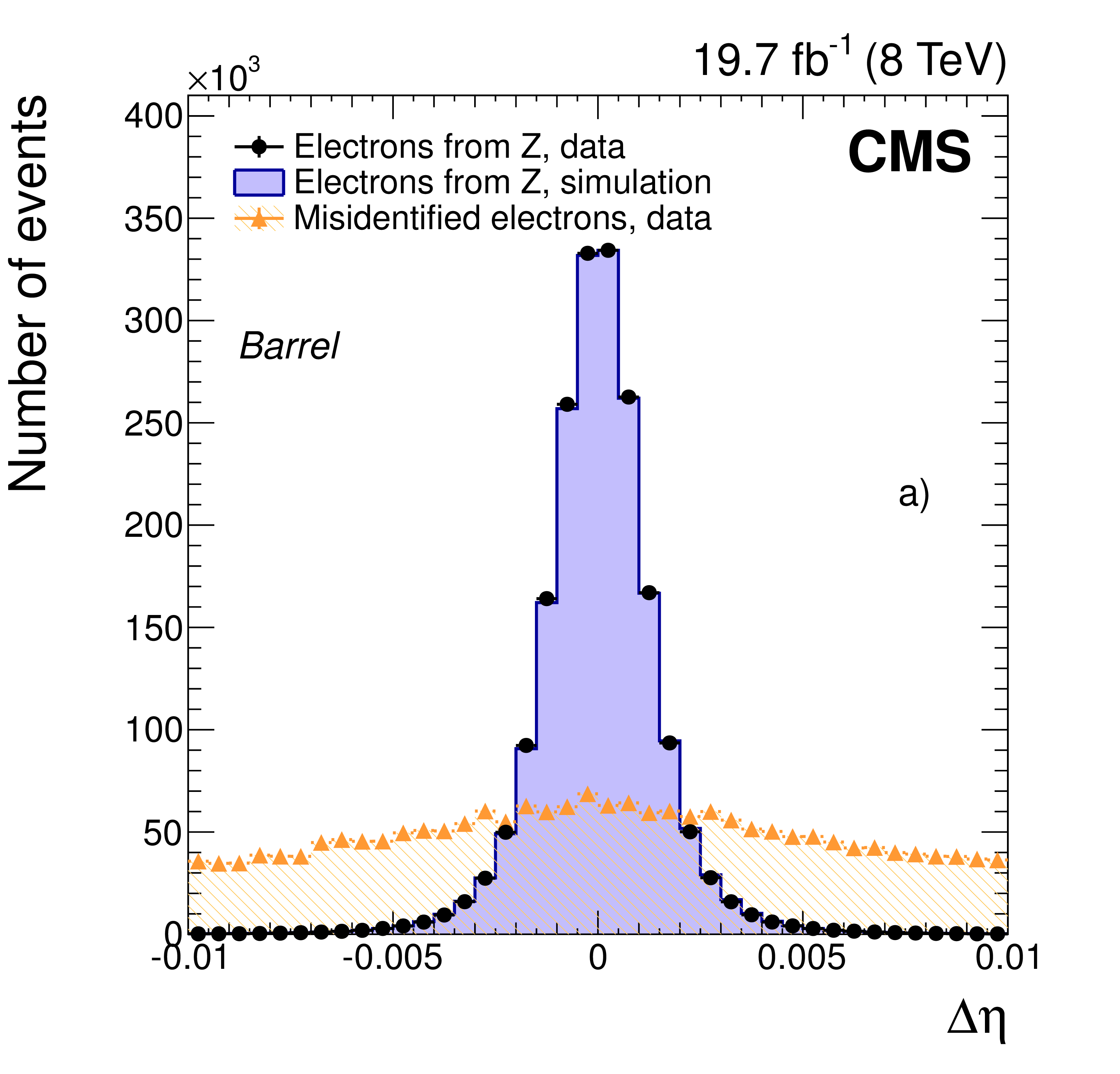
Figure 15-a:
Distributions in the distance $\Delta \eta $ between the position of the SC and the track extrapolated to the point of closest approach to the SC are shown for a) the barrel and b) the endcaps. Distributions in the shower-shape variable $\sigma _{\eta \eta }$, defined in the text, are shown in c) and d). Distributions in energy-momentum matching $1/E_{\mathrm {SC}}- 1/p$, as defined in the text, are shown in e) and f). Distributions are shown for electrons from ${\mathrm{ Z } } \to \mathrm{ e }^+ \mathrm{ e }^- $ data (dots) and simulated (solid histograms) events, and from background-enriched events in data (triangles). All distributions are normalized to their respective areas of the ${\mathrm{ Z } } \to \mathrm{ e }^+ \mathrm{ e }^- $ data. (See text for details on the samples composition.) |
png pdf |
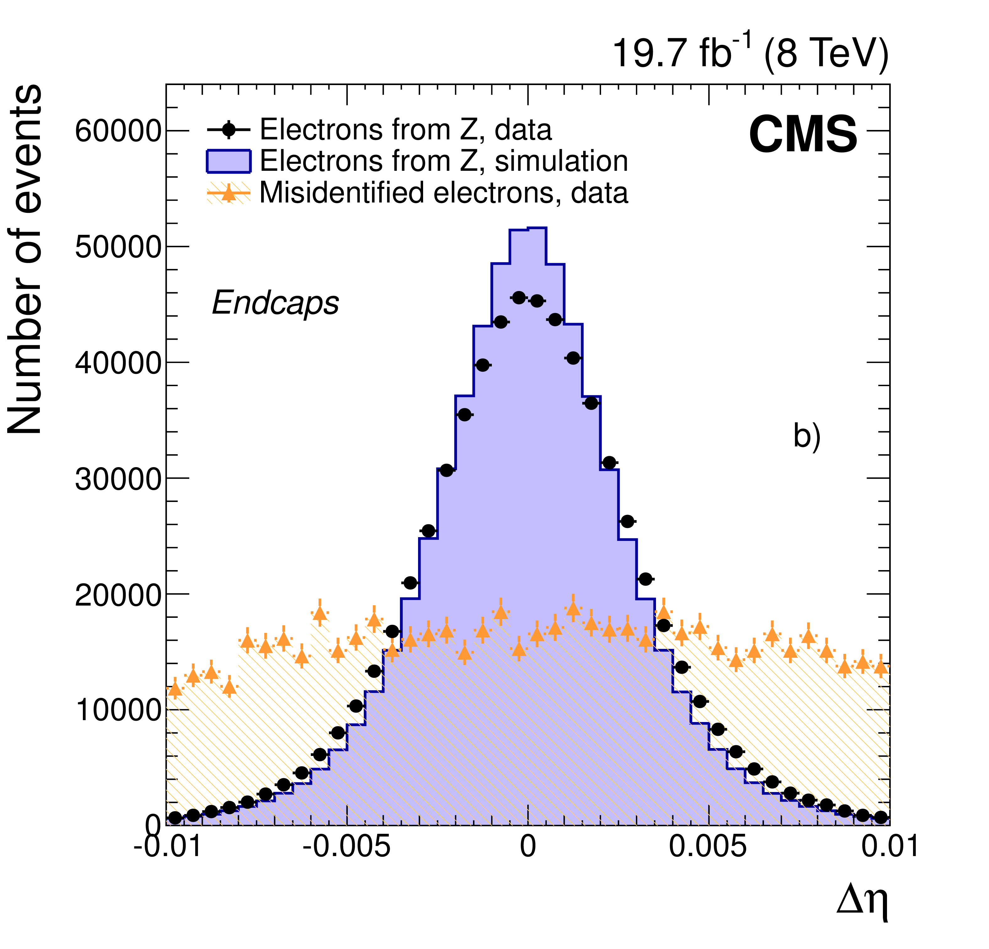
Figure 15-b:
Distributions in the distance $\Delta \eta $ between the position of the SC and the track extrapolated to the point of closest approach to the SC are shown for a) the barrel and b) the endcaps. Distributions in the shower-shape variable $\sigma _{\eta \eta }$, defined in the text, are shown in c) and d). Distributions in energy-momentum matching $1/E_{\mathrm {SC}}- 1/p$, as defined in the text, are shown in e) and f). Distributions are shown for electrons from ${\mathrm{ Z } } \to \mathrm{ e }^+ \mathrm{ e }^- $ data (dots) and simulated (solid histograms) events, and from background-enriched events in data (triangles). All distributions are normalized to their respective areas of the ${\mathrm{ Z } } \to \mathrm{ e }^+ \mathrm{ e }^- $ data. (See text for details on the samples composition.) |

png pdf |
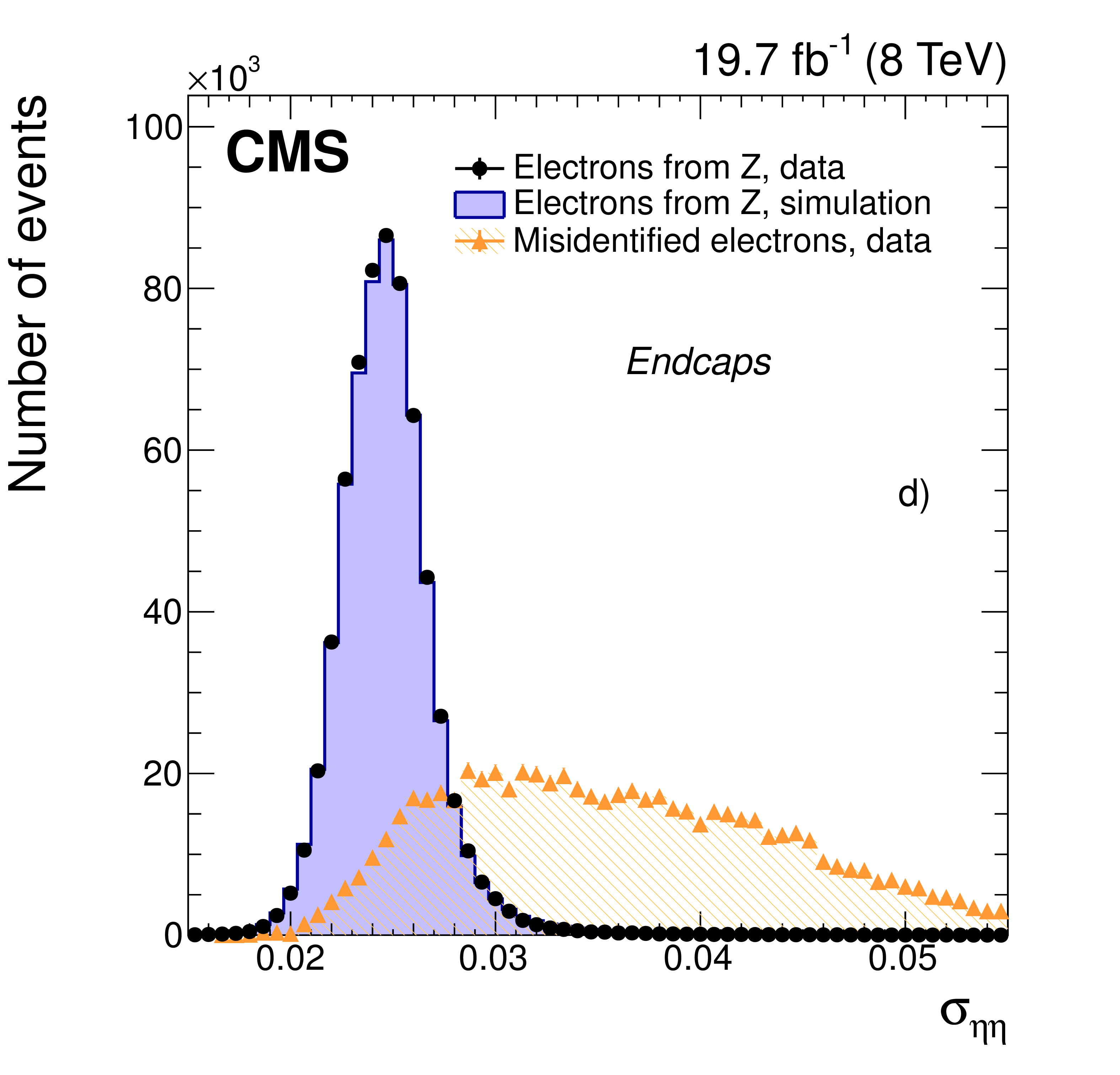
Figure 15-c:
Distributions in the distance $\Delta \eta $ between the position of the SC and the track extrapolated to the point of closest approach to the SC are shown for a) the barrel and b) the endcaps. Distributions in the shower-shape variable $\sigma _{\eta \eta }$, defined in the text, are shown in c) and d). Distributions in energy-momentum matching $1/E_{\mathrm {SC}}- 1/p$, as defined in the text, are shown in e) and f). Distributions are shown for electrons from ${\mathrm{ Z } } \to \mathrm{ e }^+ \mathrm{ e }^- $ data (dots) and simulated (solid histograms) events, and from background-enriched events in data (triangles). All distributions are normalized to their respective areas of the ${\mathrm{ Z } } \to \mathrm{ e }^+ \mathrm{ e }^- $ data. (See text for details on the samples composition.) |
png pdf |
Figure 15-d:
Distributions in the distance $\Delta \eta $ between the position of the SC and the track extrapolated to the point of closest approach to the SC are shown for a) the barrel and b) the endcaps. Distributions in the shower-shape variable $\sigma _{\eta \eta }$, defined in the text, are shown in c) and d). Distributions in energy-momentum matching $1/E_{\mathrm {SC}}- 1/p$, as defined in the text, are shown in e) and f). Distributions are shown for electrons from ${\mathrm{ Z } } \to \mathrm{ e }^+ \mathrm{ e }^- $ data (dots) and simulated (solid histograms) events, and from background-enriched events in data (triangles). All distributions are normalized to their respective areas of the ${\mathrm{ Z } } \to \mathrm{ e }^+ \mathrm{ e }^- $ data. (See text for details on the samples composition.) |
png pdf |
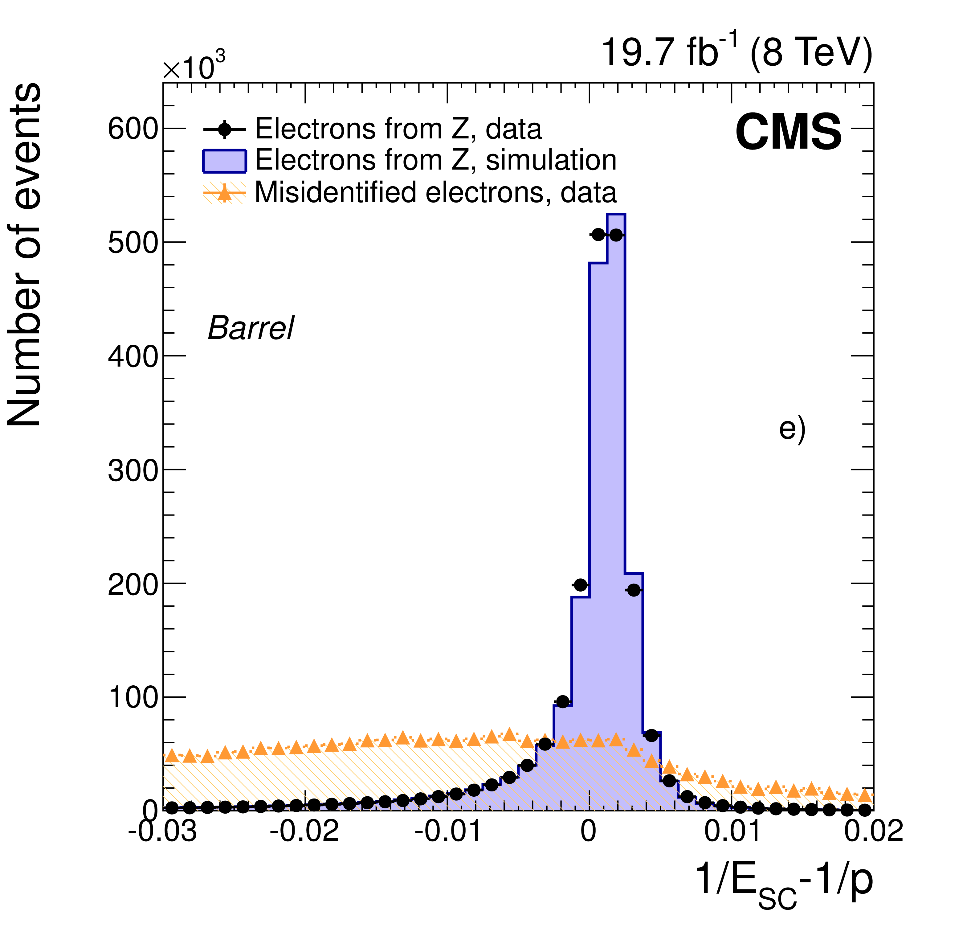
Figure 15-e:
Distributions in the distance $\Delta \eta $ between the position of the SC and the track extrapolated to the point of closest approach to the SC are shown for a) the barrel and b) the endcaps. Distributions in the shower-shape variable $\sigma _{\eta \eta }$, defined in the text, are shown in c) and d). Distributions in energy-momentum matching $1/E_{\mathrm {SC}}- 1/p$, as defined in the text, are shown in e) and f). Distributions are shown for electrons from ${\mathrm{ Z } } \to \mathrm{ e }^+ \mathrm{ e }^- $ data (dots) and simulated (solid histograms) events, and from background-enriched events in data (triangles). All distributions are normalized to their respective areas of the ${\mathrm{ Z } } \to \mathrm{ e }^+ \mathrm{ e }^- $ data. (See text for details on the samples composition.) |
png pdf |
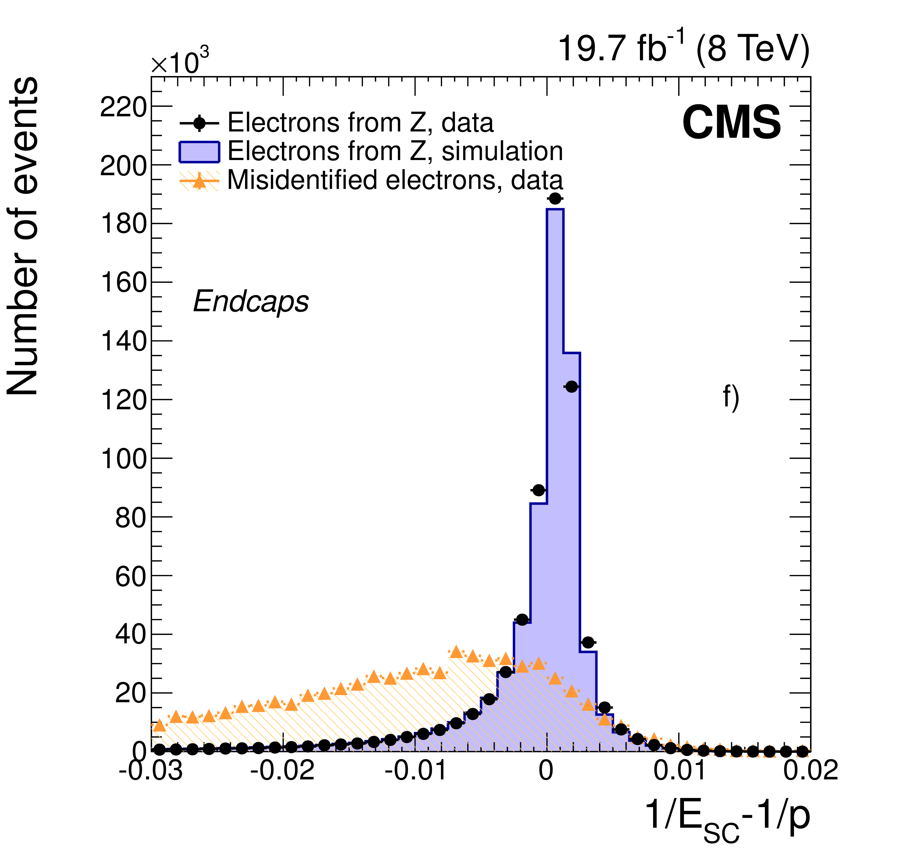
Figure 15-f:
Distributions in the distance $\Delta \eta $ between the position of the SC and the track extrapolated to the point of closest approach to the SC are shown for a) the barrel and b) the endcaps. Distributions in the shower-shape variable $\sigma _{\eta \eta }$, defined in the text, are shown in c) and d). Distributions in energy-momentum matching $1/E_{\mathrm {SC}}- 1/p$, as defined in the text, are shown in e) and f). Distributions are shown for electrons from ${\mathrm{ Z } } \to \mathrm{ e }^+ \mathrm{ e }^- $ data (dots) and simulated (solid histograms) events, and from background-enriched events in data (triangles). All distributions are normalized to their respective areas of the ${\mathrm{ Z } } \to \mathrm{ e }^+ \mathrm{ e }^- $ data. (See text for details on the samples composition.) |
png pdf |
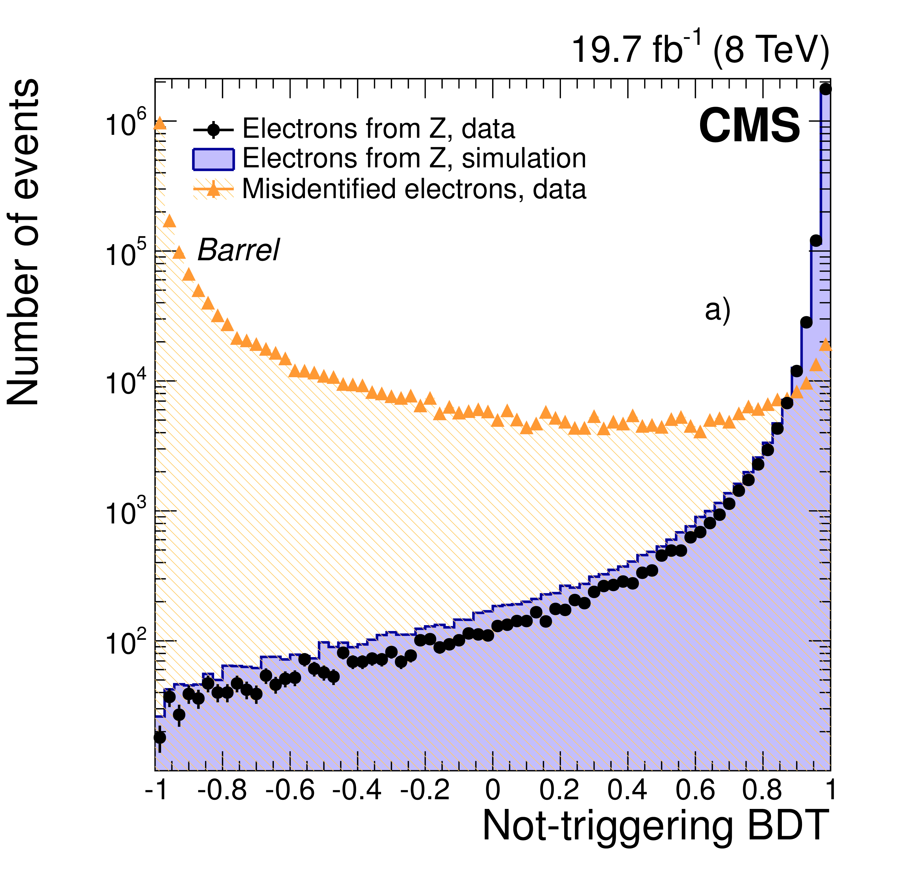
Figure 16-a:
Output of the electron-identification BDT for electrons from ${\mathrm{ Z } } \to \mathrm{ e }^+ \mathrm{ e }^- $ data (dots) and simulated (solid histograms) events, and from background-enriched events in data (triangles), in the ECAL a) barrel, and b) endcaps. All the distributions are normalized to the area of the respective ${\mathrm{ Z } } \to \mathrm{ e }^+ \mathrm{ e }^- $ data. (See text for details on the samples composition.) |
png pdf |
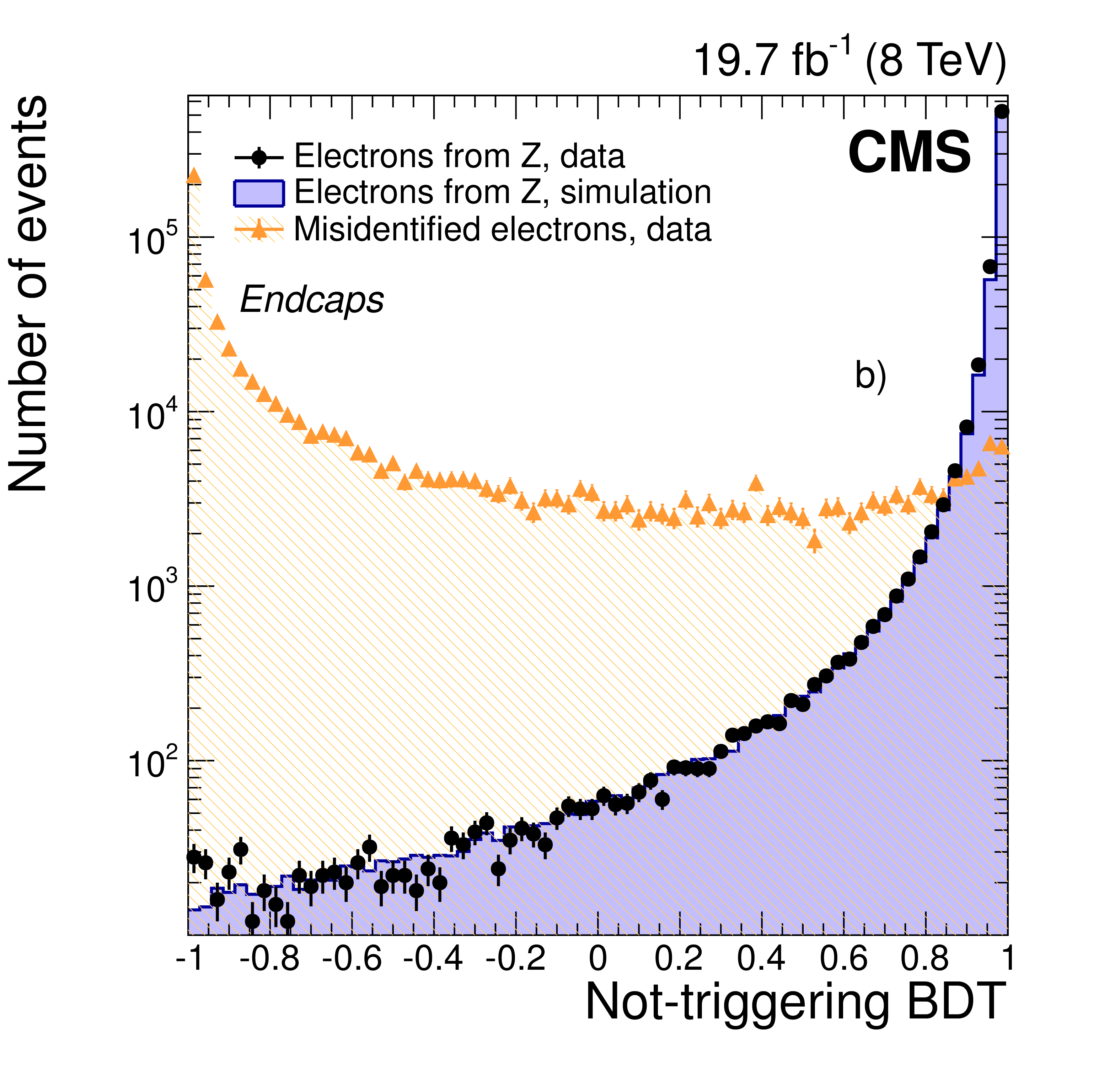
Figure 16-b:
Output of the electron-identification BDT for electrons from ${\mathrm{ Z } } \to \mathrm{ e }^+ \mathrm{ e }^- $ data (dots) and simulated (solid histograms) events, and from background-enriched events in data (triangles), in the ECAL a) barrel, and b) endcaps. All the distributions are normalized to the area of the respective ${\mathrm{ Z } } \to \mathrm{ e }^+ \mathrm{ e }^- $ data. (See text for details on the samples composition.) |
png |
Figure 17-a:
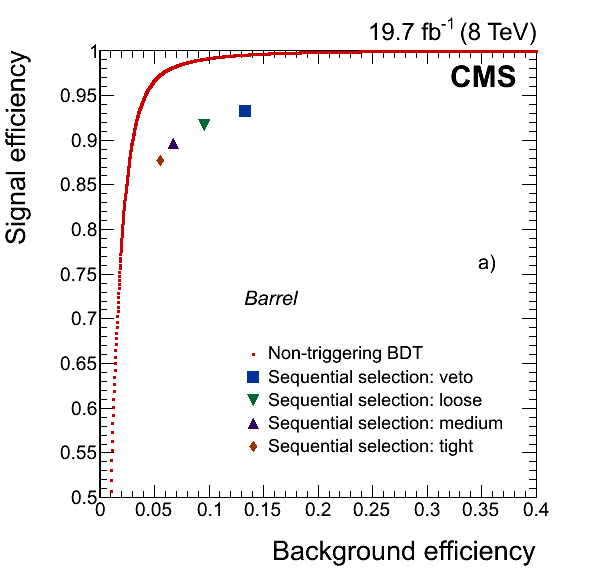
Performance of the electron BDT-based identification algorithm (red dots) compared with results from working points of the sequential selection (only the identification part) for electron candidates in the ECAL a) barrel, and b) endcaps. (See text for details on the samples composition.) |
png |
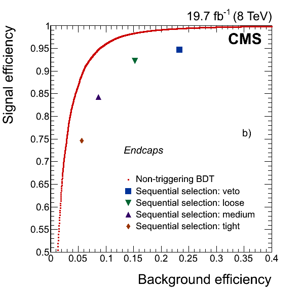
Figure 17-b:
Performance of the electron BDT-based identification algorithm (red dots) compared with results from working points of the sequential selection (only the identification part) for electron candidates in the ECAL a) barrel, and b) endcaps. (See text for details on the samples composition.) |
png pdf |
Figure 18-a:
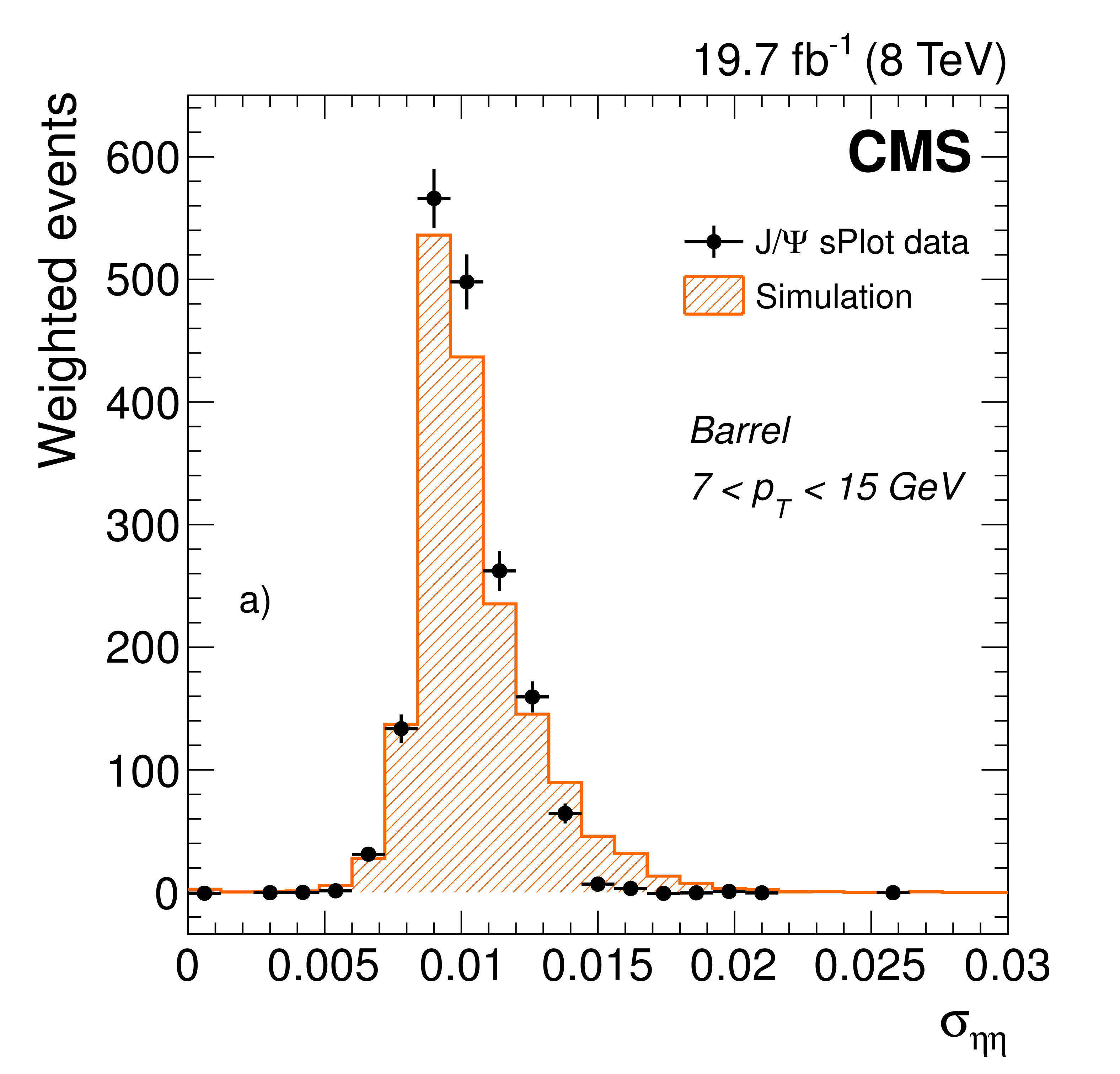
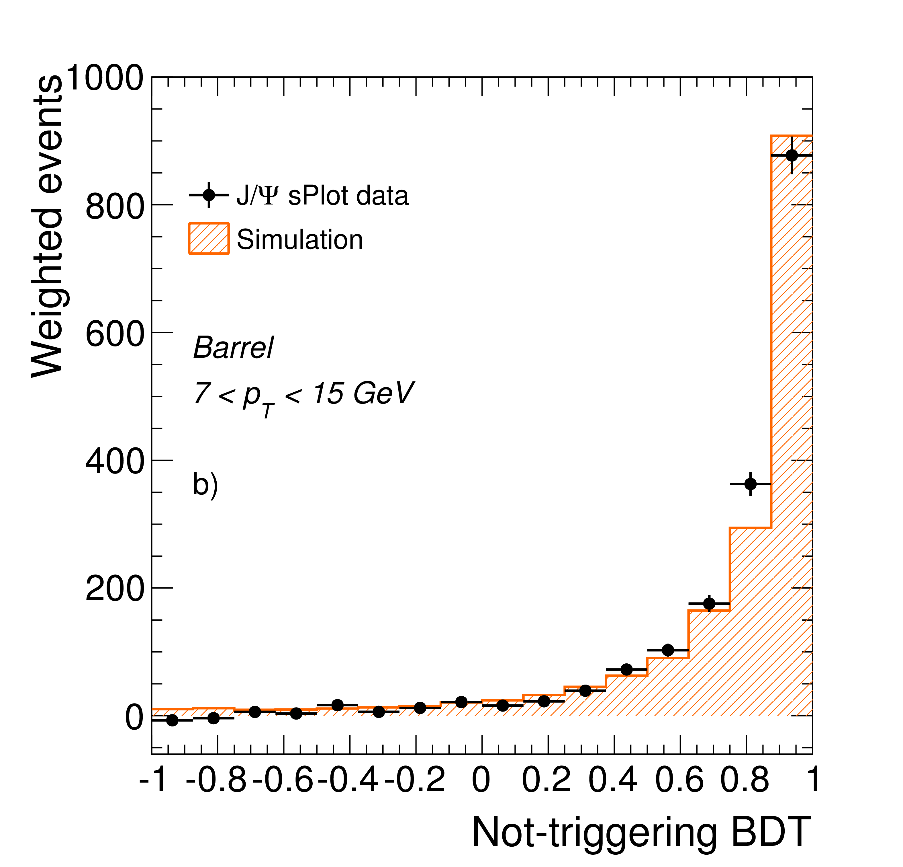
Distribution of a) the shower-shape variable $\sigma _{\eta \eta }$, defined in the text, and b) the output of the BDT electron identification algorithm for electron candidates in the ECAL barrel, in data (symbols) and simulation (histograms). A statistical subtraction of the background is applied using the sPlot technique. (See text for details.) |
png pdf |
Figure 18-b:
Distribution of a) the shower-shape variable $\sigma _{\eta \eta }$, defined in the text, and b) the output of the BDT electron identification algorithm for electron candidates in the ECAL barrel, in data (symbols) and simulation (histograms). A statistical subtraction of the background is applied using the sPlot technique. (See text for details.) |
png |
Figure 19-a:
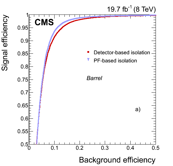
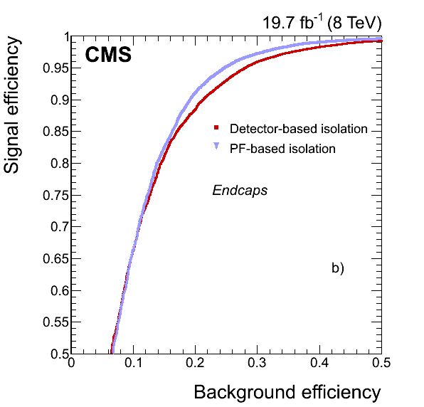
Performance of the detector-based isolation algorithm (red squares) compared with that using PF (blue triangles) in the ECAL a) barrel, and b) endcaps. (See text for the definition of the samples.) |
png |
Figure 19-b:
Performance of the detector-based isolation algorithm (red squares) compared with that using PF (blue triangles) in the ECAL a) barrel, and b) endcaps. (See text for the definition of the samples.) |
png pdf |
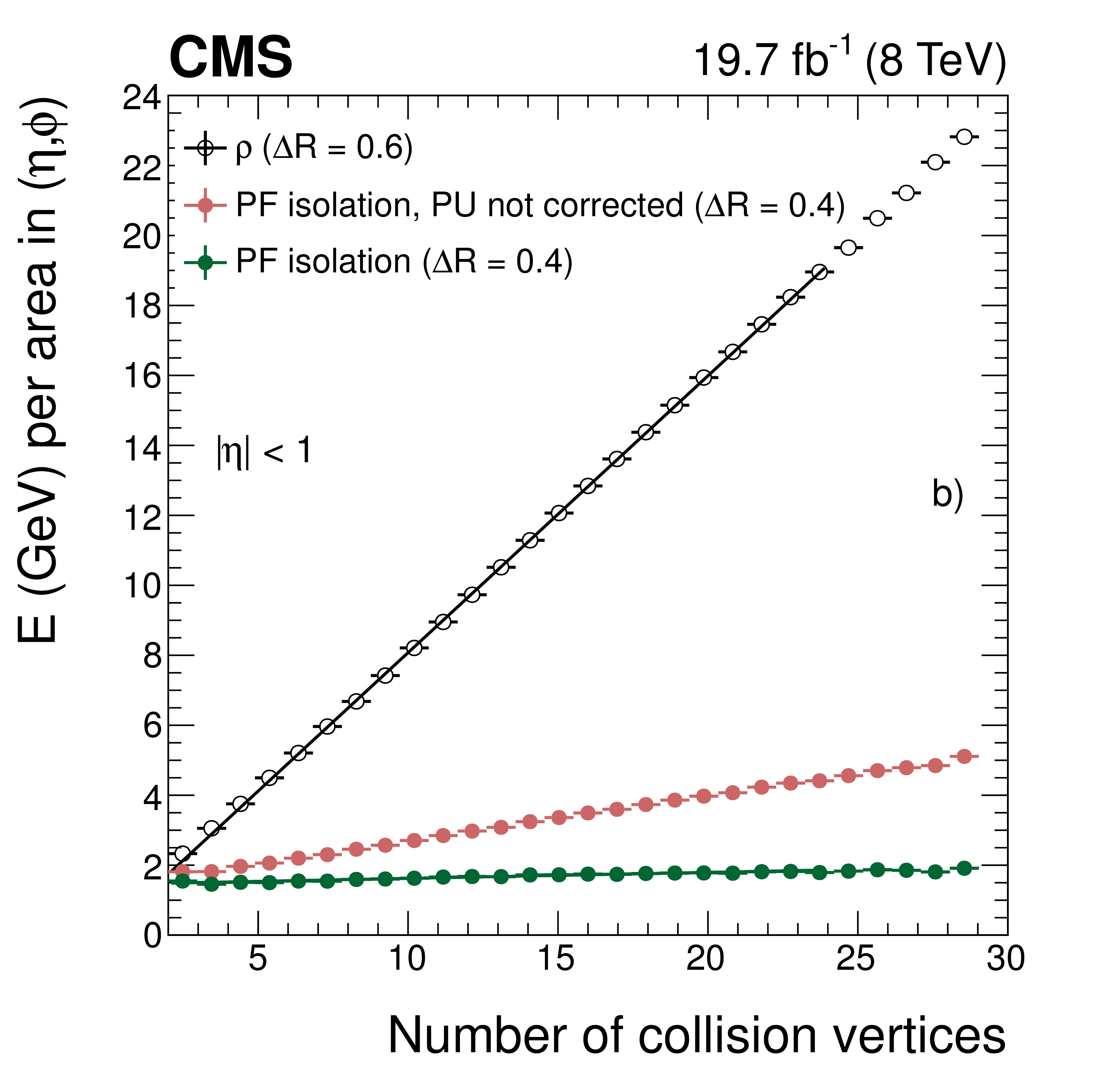
Figure 20-a:
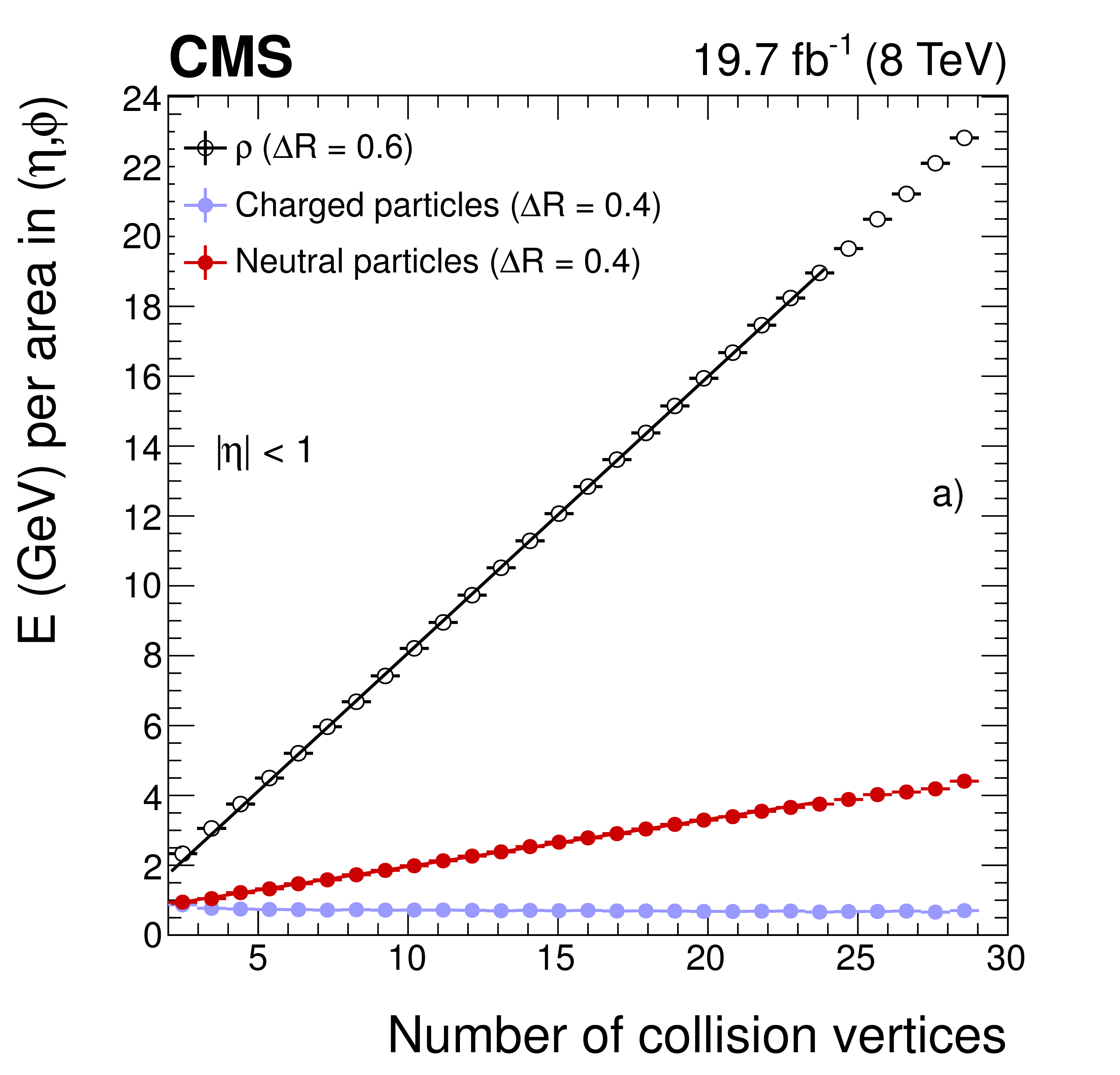
Average energy density as a function of the number of reconstructed proton-proton collision vertices, for electron candidates with $ {p_{\mathrm {T}}} >$ 20 GeV and $ {| \eta | }< $ 1 from data dominated by ${\mathrm{ Z } } \to \mathrm{ e }^+ \mathrm{ e }^- $ events. The energy density $\rho $ (open dots) is shown, along with each component of the particle isolation: a) neutral particles (red dots) and charged particles associated with the vertex (blue dots), and b) before (pink dots) and after (green dots) the correction for pileup on PF isolation. |
png pdf |
Figure 20-b:
Average energy density as a function of the number of reconstructed proton-proton collision vertices, for electron candidates with $ {p_{\mathrm {T}}} >$ 20 GeV and $ {| \eta | }< $ 1 from data dominated by ${\mathrm{ Z } } \to \mathrm{ e }^+ \mathrm{ e }^- $ events. The energy density $\rho $ (open dots) is shown, along with each component of the particle isolation: a) neutral particles (red dots) and charged particles associated with the vertex (blue dots), and b) before (pink dots) and after (green dots) the correction for pileup on PF isolation. |
png pdf |
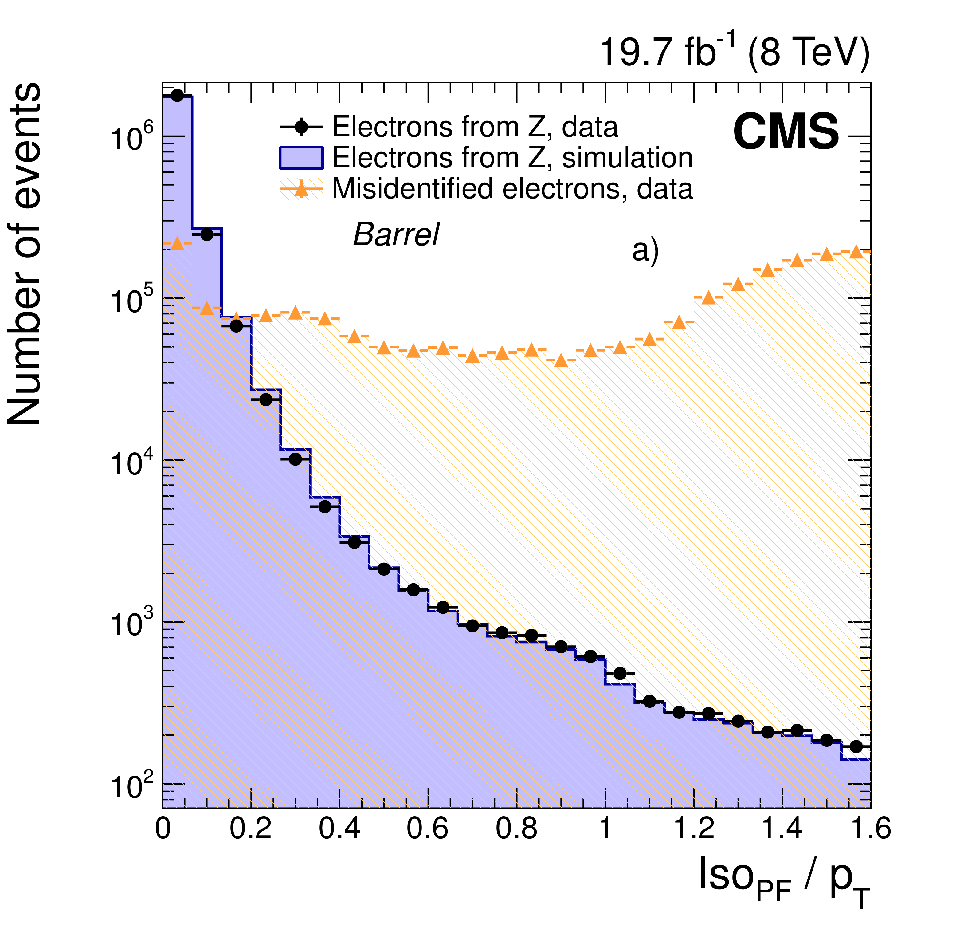
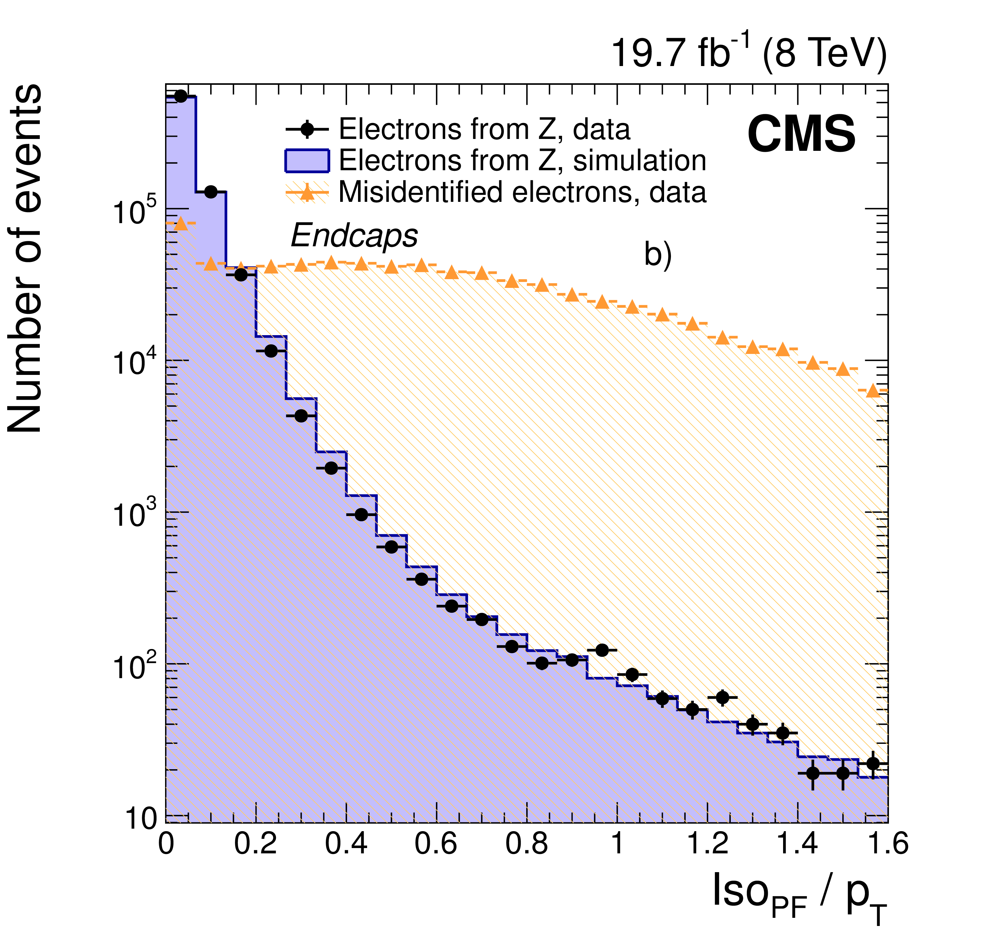
Figure 21-a:
Distributions of PF isolation divided by electron ${p_{\mathrm {T}}} $, after applying the pileup correction discussed in the text, for electrons from ${\mathrm{ Z } } \to \mathrm{ e }^+ \mathrm{ e }^- $ data (dots) and simulated (solid histograms) events, and from background-enriched events in data (triangles), in the ECAL a) barrel, and b) endcaps. (See text for more details on the compositions of the samples.) |
png pdf |
Figure 21-b:
Distributions of PF isolation divided by electron ${p_{\mathrm {T}}} $, after applying the pileup correction discussed in the text, for electrons from ${\mathrm{ Z } } \to \mathrm{ e }^+ \mathrm{ e }^- $ data (dots) and simulated (solid histograms) events, and from background-enriched events in data (triangles), in the ECAL a) barrel, and b) endcaps. (See text for more details on the compositions of the samples.) |
png pdf |
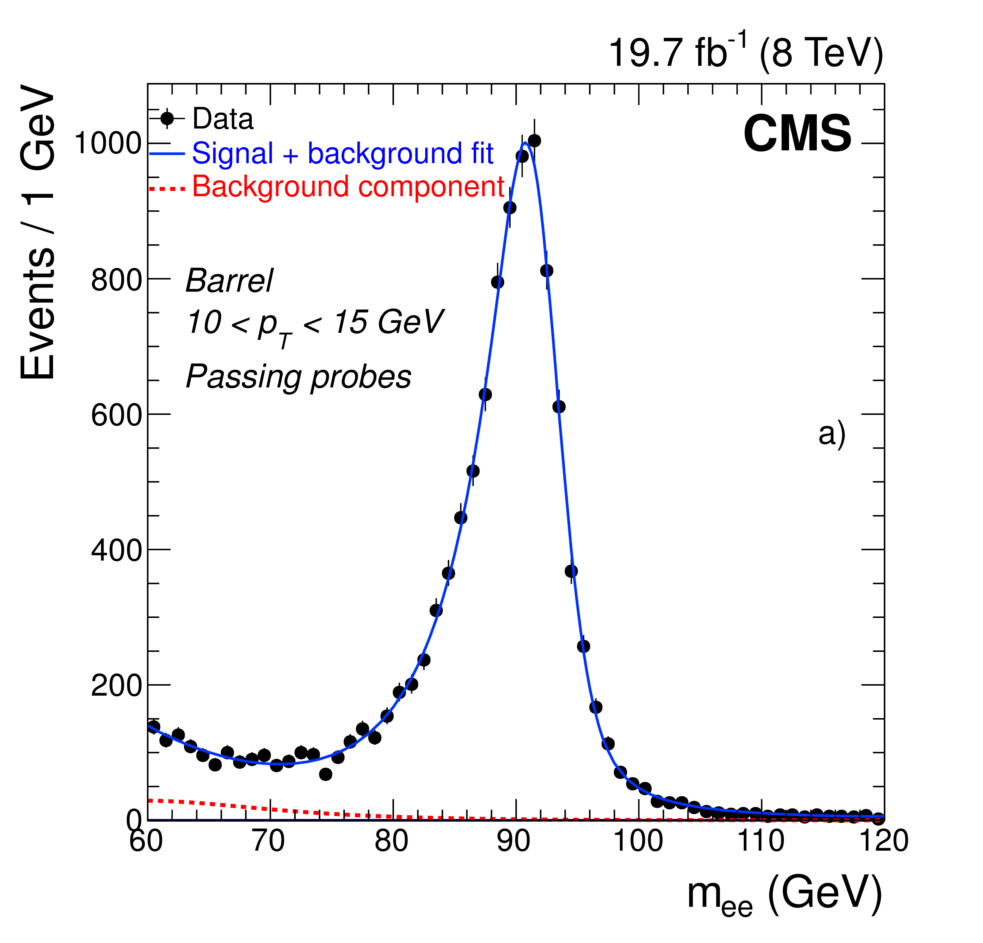
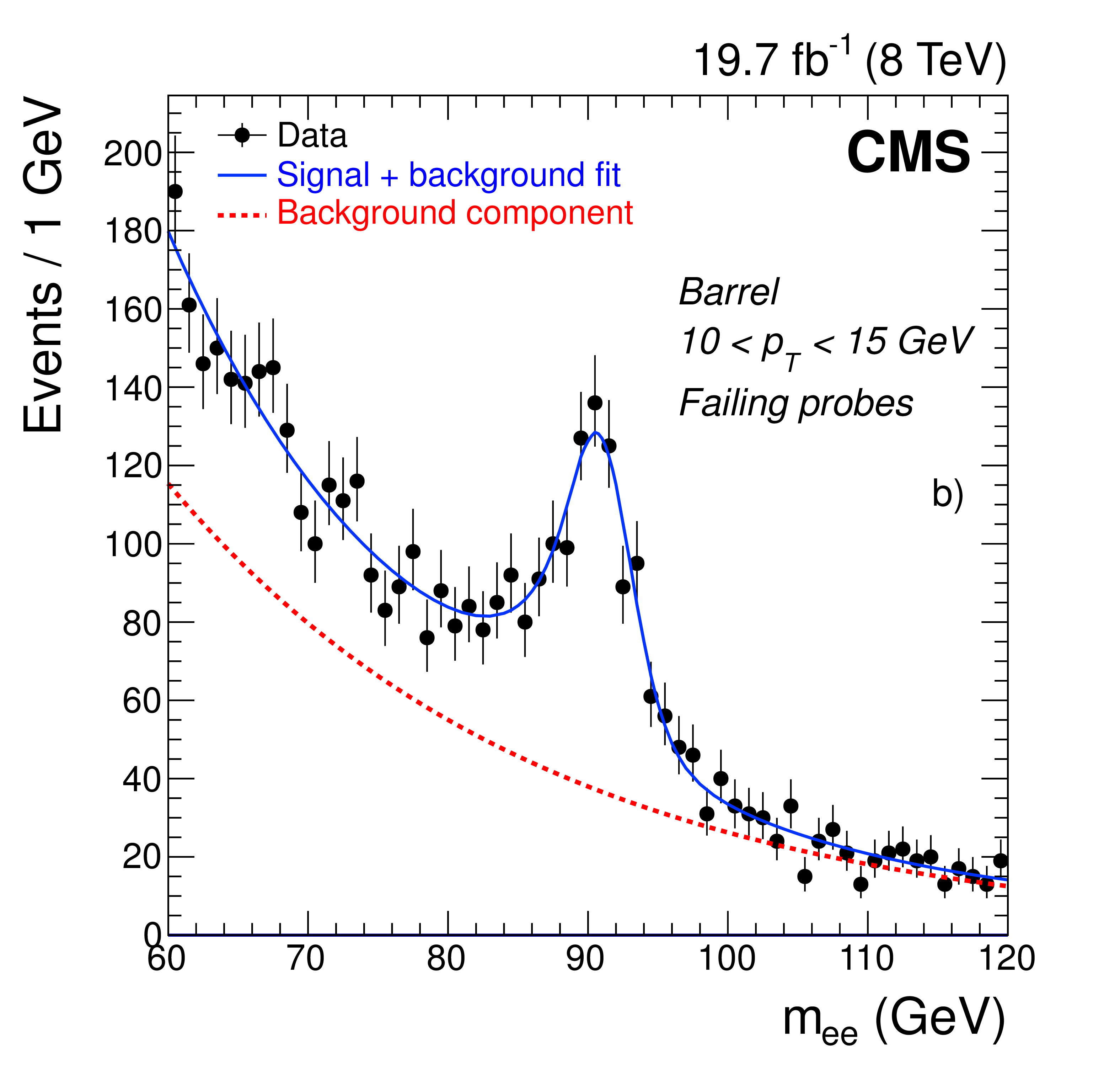
Figure 22-a:
Example of fits to dielectron invariant mass distributions for probe electrons with 10 $< {p_{\mathrm {T}}} <$ 15 GeV in the ECAL barrel that a) pass or b) fail the selections on isolation and impact parameter of the MVA selection used in Ref. [9]. Fits are shown for the signal+background hypothesis (full line), and for the background component alone (dashed line). |
png pdf |
Figure 22-b:
Example of fits to dielectron invariant mass distributions for probe electrons with 10 $< {p_{\mathrm {T}}} <$ 15 GeV in the ECAL barrel that a) pass or b) fail the selections on isolation and impact parameter of the MVA selection used in Ref. [9]. Fits are shown for the signal+background hypothesis (full line), and for the background component alone (dashed line). |
png pdf |
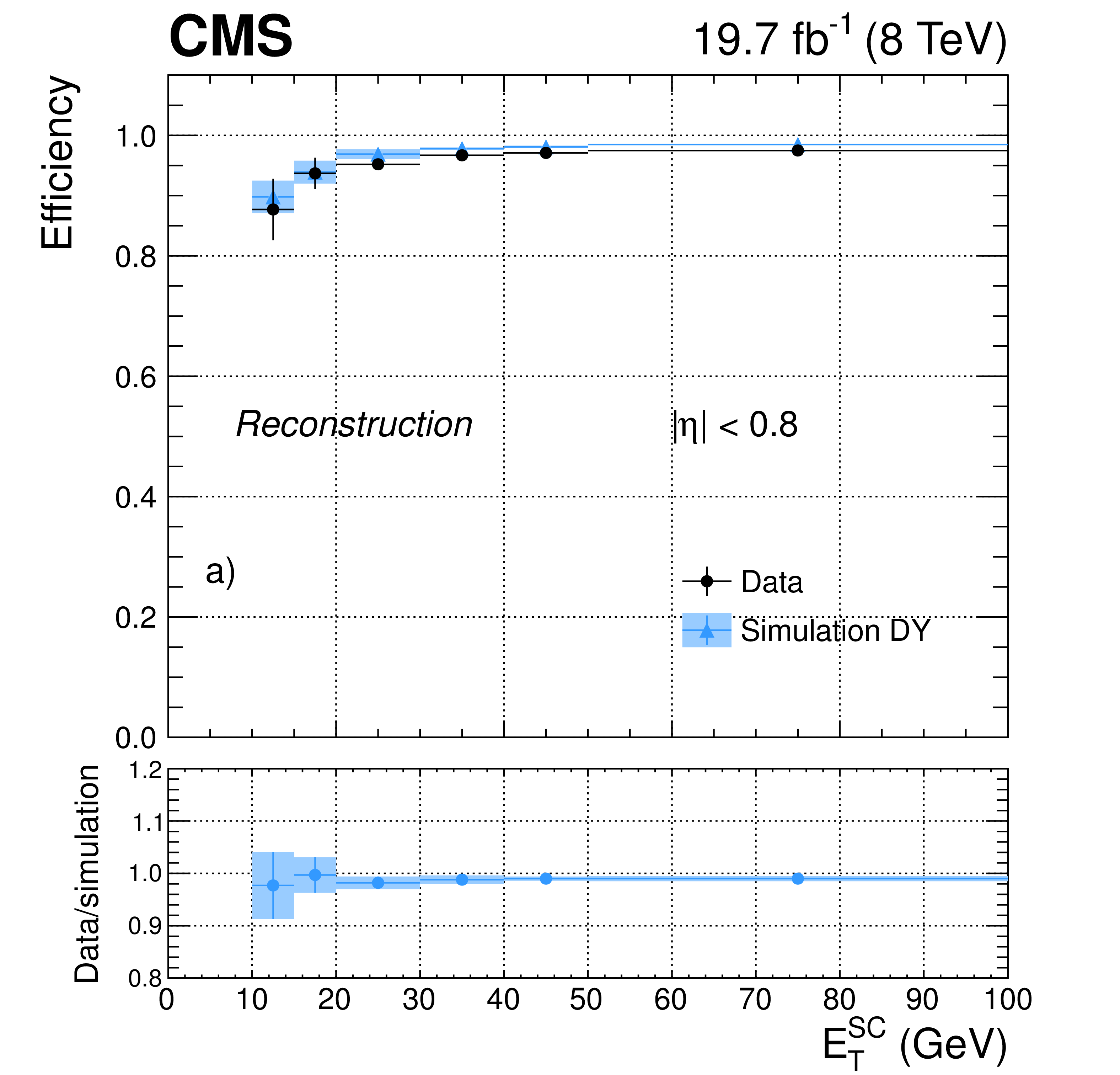
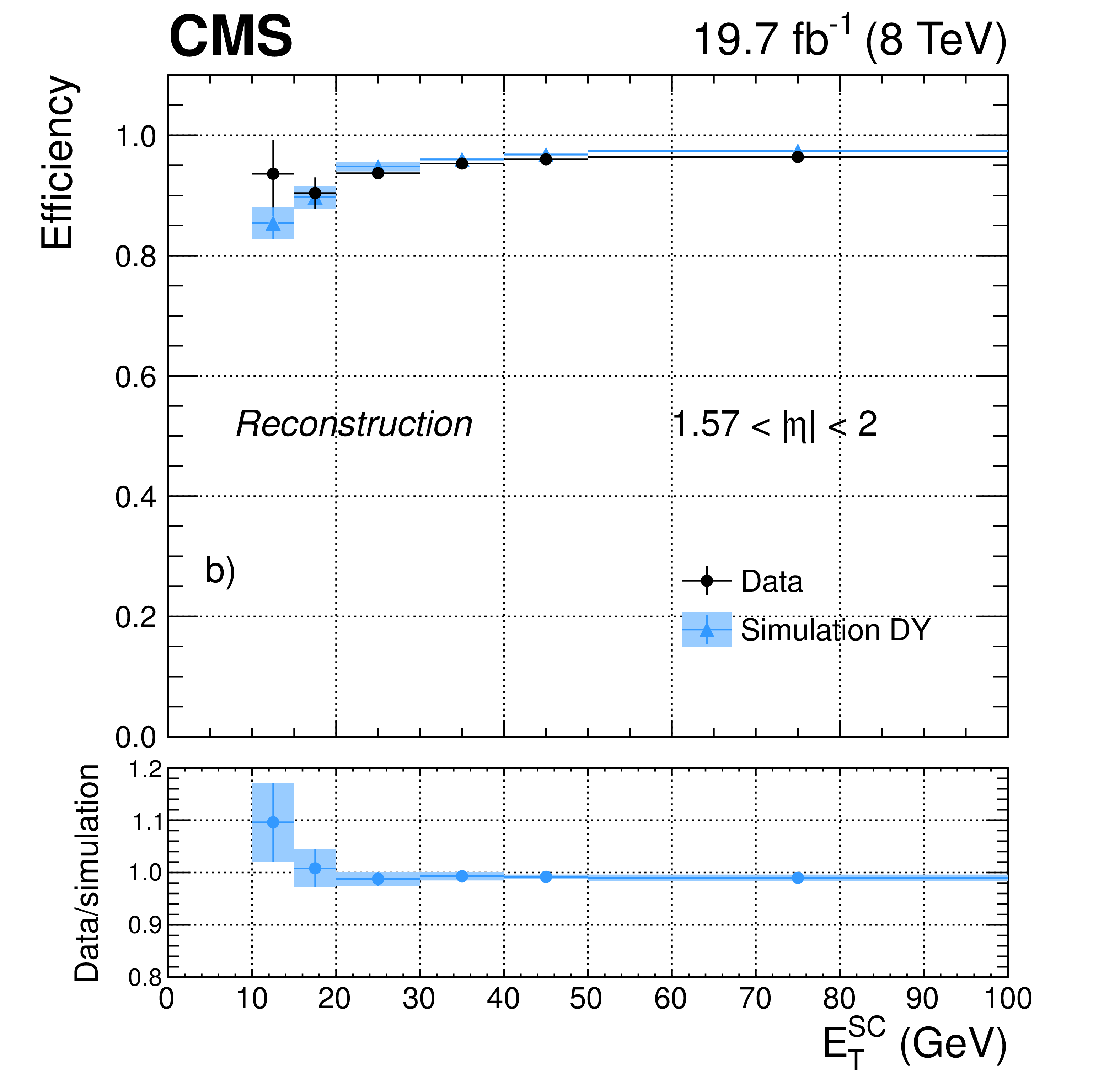
Figure 23-a:
Electron reconstruction efficiency measured in dielectron events in data (dots) and DY simulation (triangles), as a function of the electron $ {E_{\mathrm {T}}} ^{\mathrm {SC}}$ for a) $ {| \eta | }<$ 0.8, and b) 1.57 $< {| \eta | }<$ 2. The bottom panels show the corresponding data-to-simulation scale factors. The uncertainties shown in the plots correspond to the quadratic sum of the statistical and systematic contributions. |
png pdf |
Figure 23-b:
Electron reconstruction efficiency measured in dielectron events in data (dots) and DY simulation (triangles), as a function of the electron $ {E_{\mathrm {T}}} ^{\mathrm {SC}}$ for a) $ {| \eta | }<$ 0.8, and b) 1.57 $< {| \eta | }<$ 2. The bottom panels show the corresponding data-to-simulation scale factors. The uncertainties shown in the plots correspond to the quadratic sum of the statistical and systematic contributions. |
png pdf |
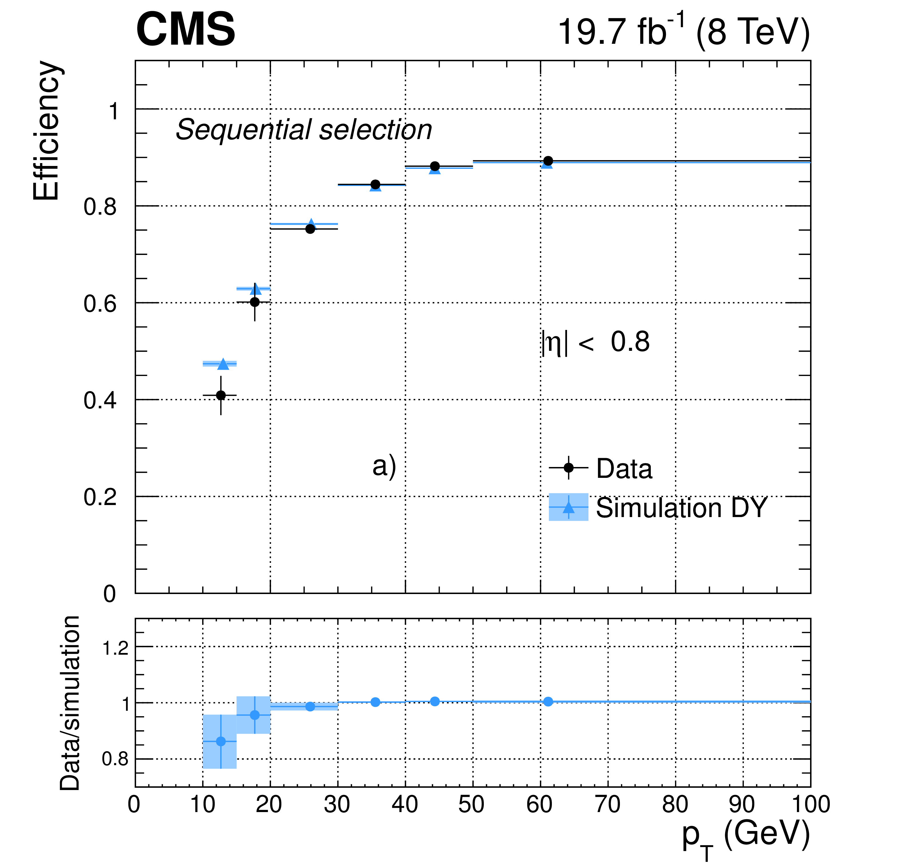
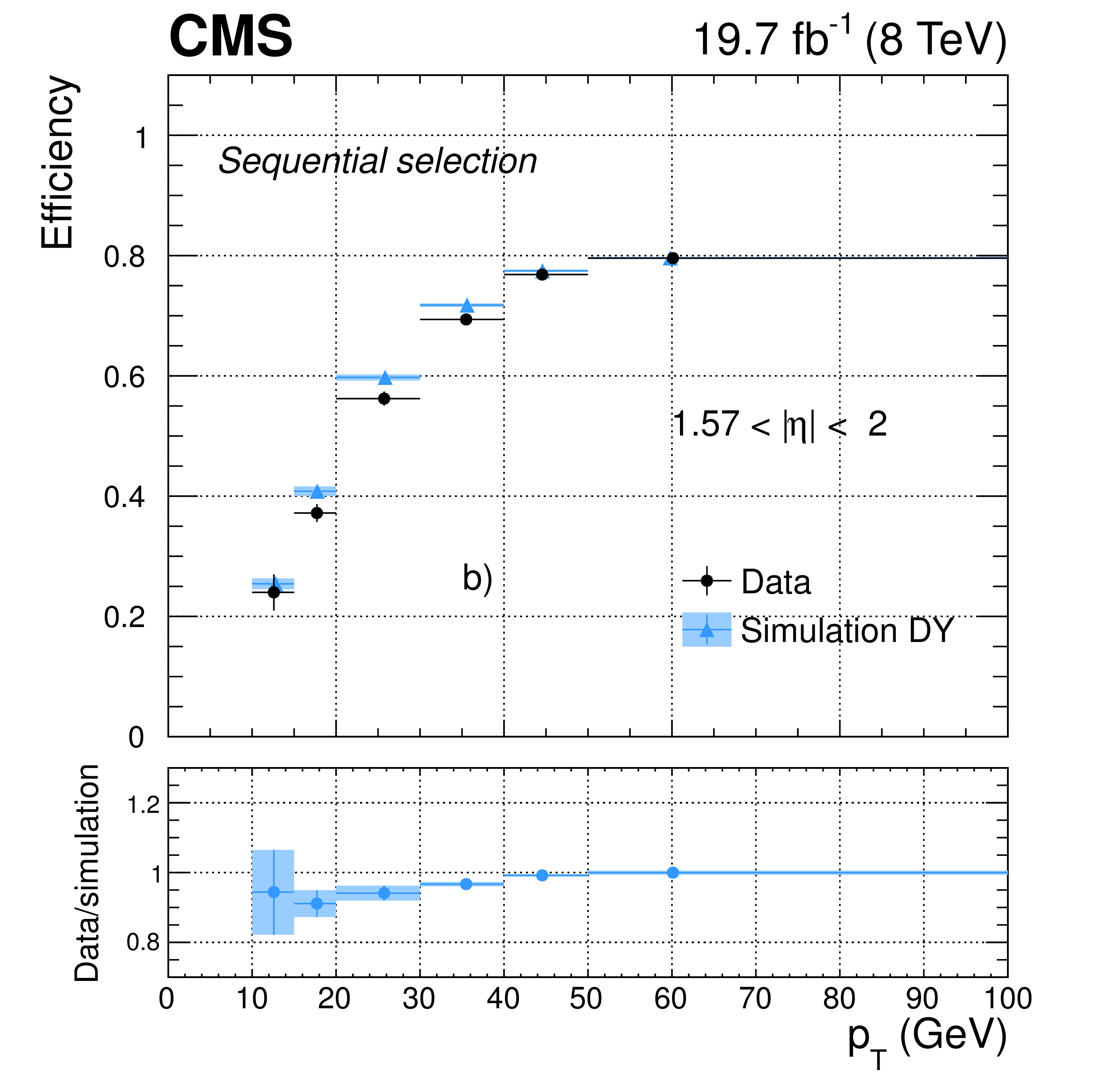
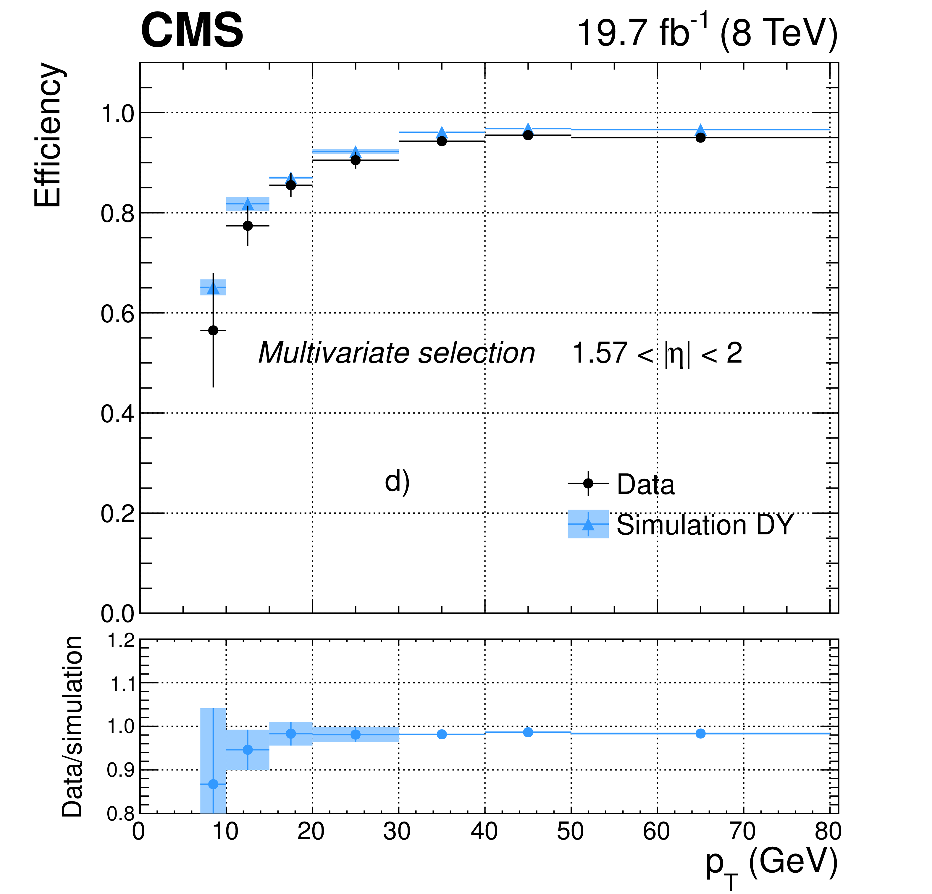
Figure 24-a:
Efficiency as a function of electron $ {p_{\mathrm {T}}} $ for dielectron events in data (dots) and DY simulation (triangles), for the medium working point of the sequential selection in a) $ {| \eta | }<$ 0.8, and b) 1.57 $< {| \eta | }<$ 2; and for the MVA selection used in Ref. [9] in c) $ {| \eta | }<$ 0.8, and d) 1.57 $< {| \eta | }<$ 2. The corresponding data-to-simulation scale factors are shown in the bottom panels of each plot. The uncertainties shown in the plots correspond to the quadratic sum of the statistical and systematic contributions. |
png pdf |
Figure 24-b:
Efficiency as a function of electron $ {p_{\mathrm {T}}} $ for dielectron events in data (dots) and DY simulation (triangles), for the medium working point of the sequential selection in a) $ {| \eta | }<$ 0.8, and b) 1.57 $< {| \eta | }<$ 2; and for the MVA selection used in Ref. [9] in c) $ {| \eta | }<$ 0.8, and d) 1.57 $< {| \eta | }<$ 2. The corresponding data-to-simulation scale factors are shown in the bottom panels of each plot. The uncertainties shown in the plots correspond to the quadratic sum of the statistical and systematic contributions. |

png pdf |
Figure 24-c:
Efficiency as a function of electron $ {p_{\mathrm {T}}} $ for dielectron events in data (dots) and DY simulation (triangles), for the medium working point of the sequential selection in a) $ {| \eta | }<$ 0.8, and b) 1.57 $< {| \eta | }<$ 2; and for the MVA selection used in Ref. [9] in c) $ {| \eta | }<$ 0.8, and d) 1.57 $< {| \eta | }<$ 2. The corresponding data-to-simulation scale factors are shown in the bottom panels of each plot. The uncertainties shown in the plots correspond to the quadratic sum of the statistical and systematic contributions. |
png pdf |
Figure 24-d:
Efficiency as a function of electron $ {p_{\mathrm {T}}} $ for dielectron events in data (dots) and DY simulation (triangles), for the medium working point of the sequential selection in a) $ {| \eta | }<$ 0.8, and b) 1.57 $< {| \eta | }<$ 2; and for the MVA selection used in Ref. [9] in c) $ {| \eta | }<$ 0.8, and d) 1.57 $< {| \eta | }<$ 2. The corresponding data-to-simulation scale factors are shown in the bottom panels of each plot. The uncertainties shown in the plots correspond to the quadratic sum of the statistical and systematic contributions. |
png pdf |
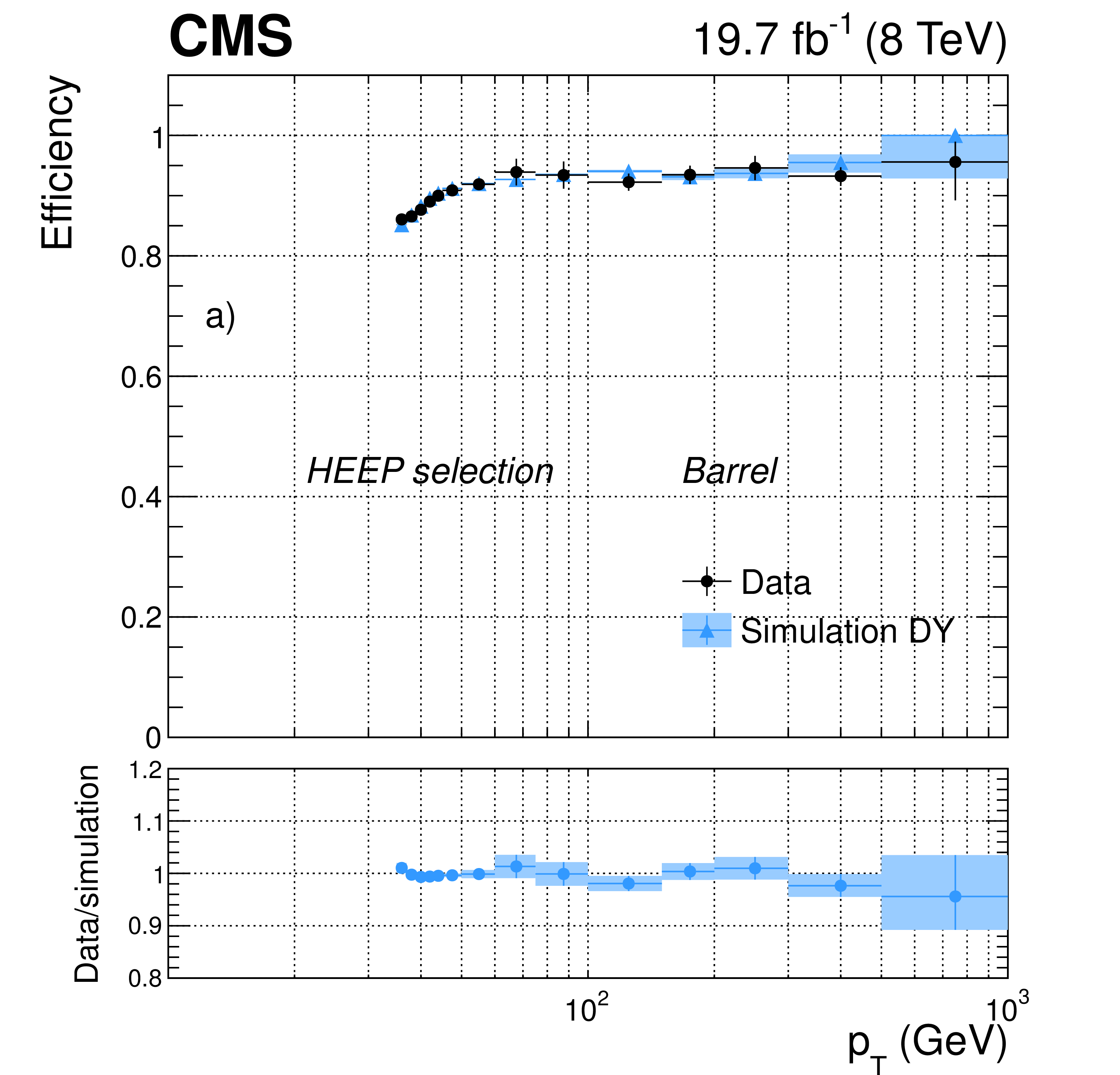
Figure 25-a:
Efficiency of the HEEP selection as a function of electron $ {p_{\mathrm {T}}} $ for dielectron events in data (dots) and DY simulation (triangles) in the ECAL a) barrel, and b) endcaps. The uncertainties shown in the plots correspond to the quadratic sum of the statistical and systematic contributions. |
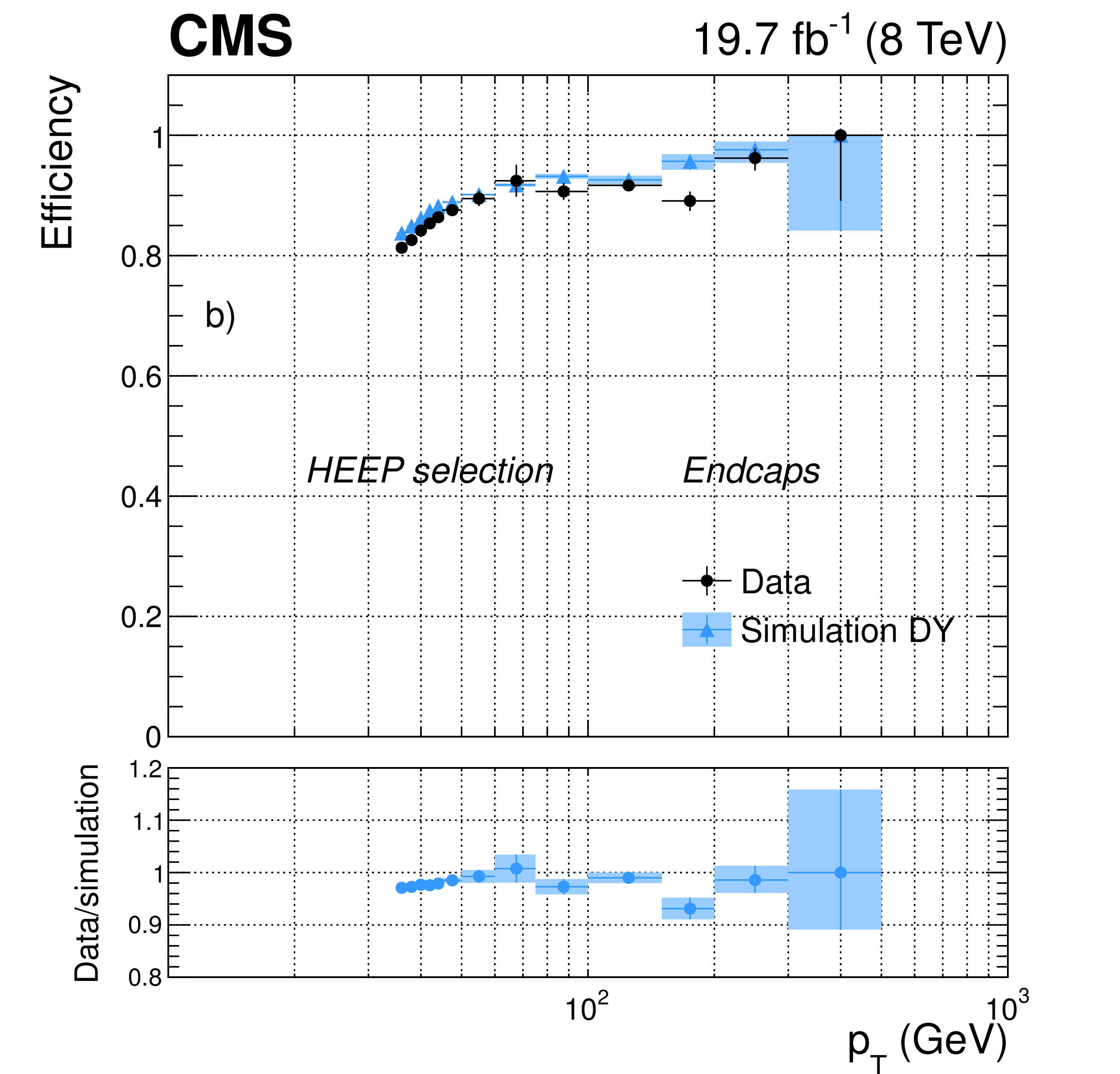
png pdf |
Figure 25-b:
Efficiency of the HEEP selection as a function of electron $ {p_{\mathrm {T}}} $ for dielectron events in data (dots) and DY simulation (triangles) in the ECAL a) barrel, and b) endcaps. The uncertainties shown in the plots correspond to the quadratic sum of the statistical and systematic contributions. |
png pdf |
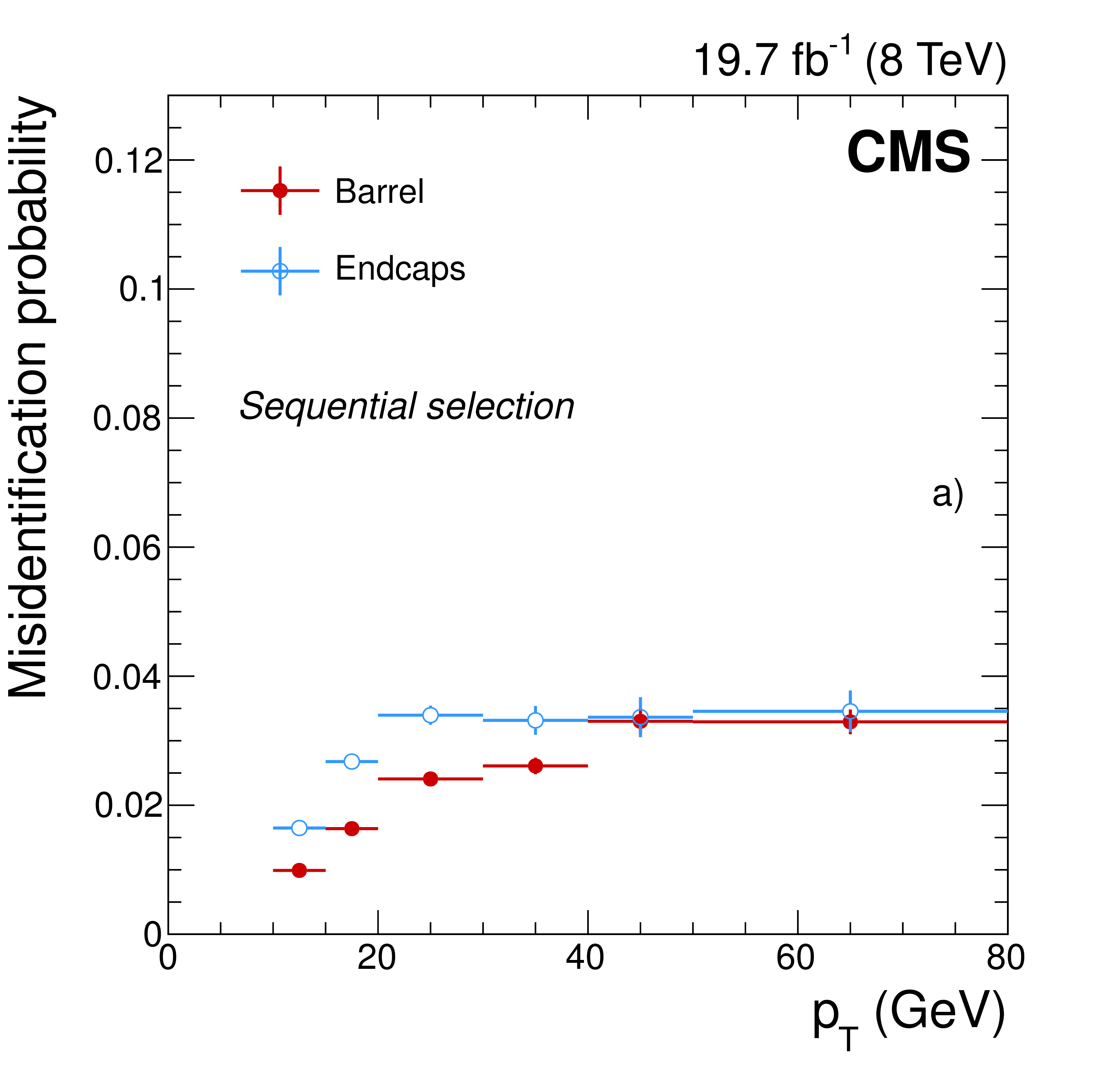
Figure 26-a:
Misidentification probability, measured in data as described in the text, as a function of the electron $ {p_{\mathrm {T}}} $ in the barrel (red dots) and endcaps (blue dots) for candidates passing a) the medium working point of the sequential selection, and b) the working point of the MVA selection used in Ref. [9]. The uncertainties shown in the plots correspond to just the statistical contributions. |
png pdf |
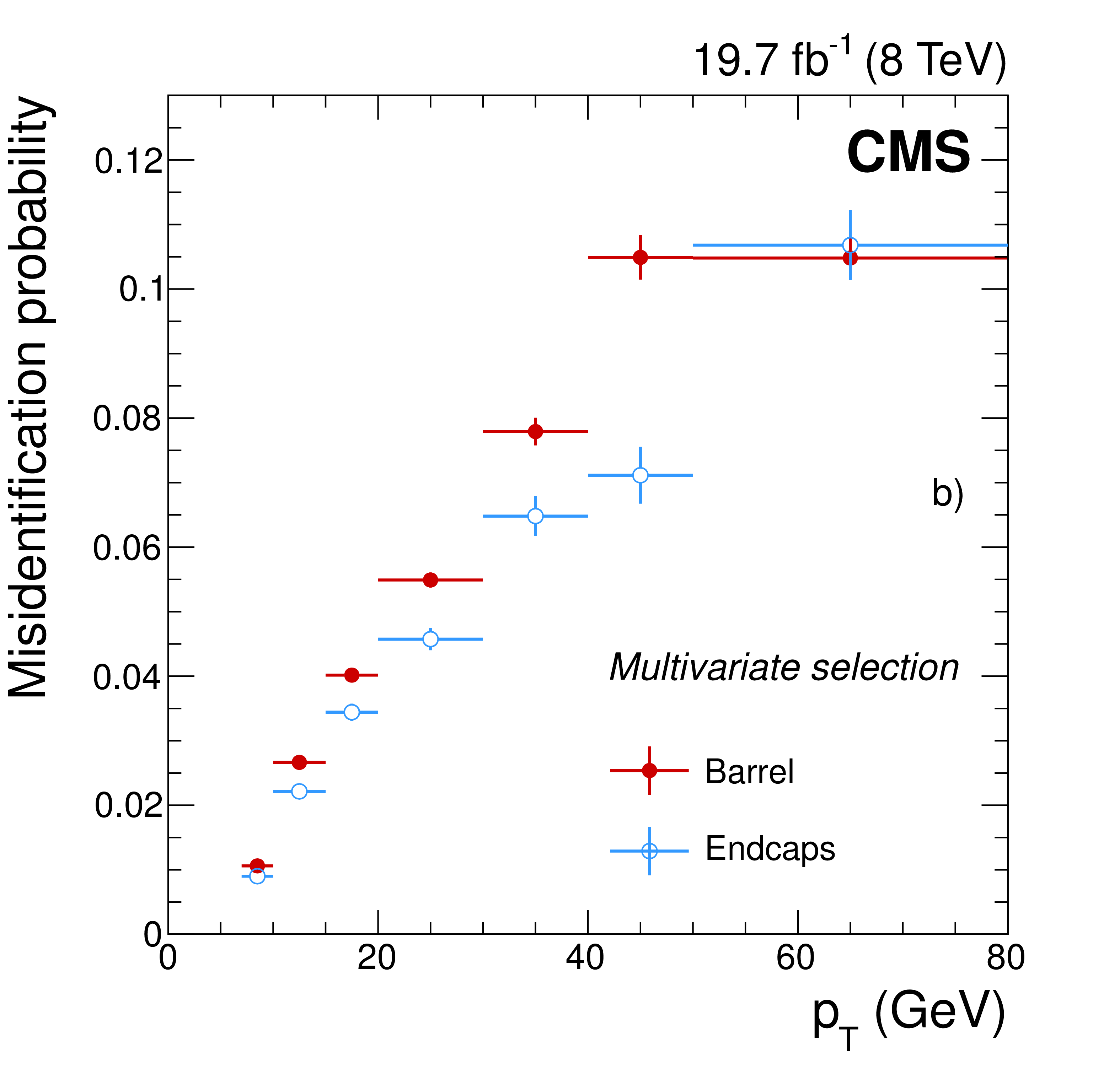
Figure 26-b:
Misidentification probability, measured in data as described in the text, as a function of the electron $ {p_{\mathrm {T}}} $ in the barrel (red dots) and endcaps (blue dots) for candidates passing a) the medium working point of the sequential selection, and b) the working point of the MVA selection used in Ref. [9]. The uncertainties shown in the plots correspond to just the statistical contributions. |
| Tables | |
png pdf |
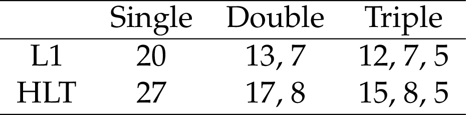
Table 1:
Lowest, unprescaled $ {E_{\mathrm {T}}} $ threshold values in GeV used for the L1 and HLT single-, double- and triple-electron triggers. |
png pdf |
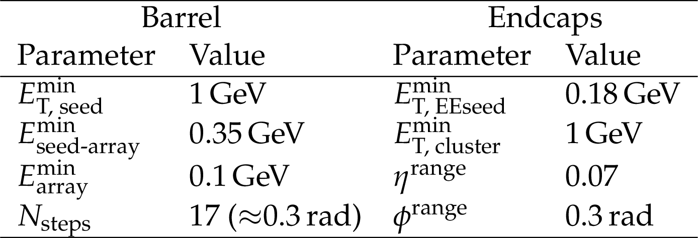
Table 2:
Threshold values of parameters used in the hybrid superclustering algorithm in the barrel, and in the multi-5$\times $5 superclustering algorithm in the endcaps. |
png pdf |
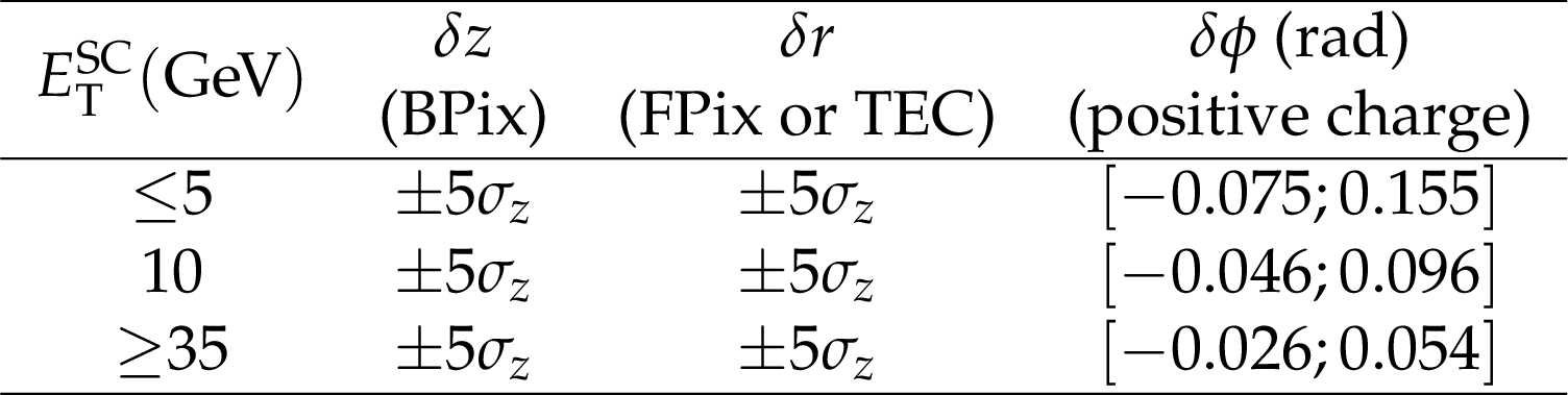
Table 3:
Values of the $\delta z$, $\delta r$ and $\delta \phi $ parameters used for the first window of seed selection, for three ranges of $ {E_{\mathrm {T}}} ^{\mathrm {SC}}$, with $\sigma _z$ being the standard deviation of the beam spot along the $z$ axis. For electron candidates with negative charge, the same $\delta \phi $ window is used, but with opposite signs. |
png pdf |
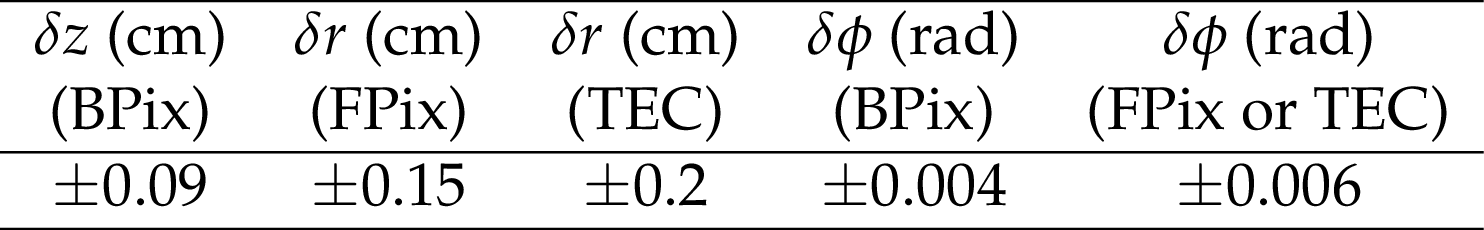
Table 4:
Values of the $\delta z$, $\delta r$ and $\delta \phi $ parameters used in different regions of the tracker for the second window of seed selection. |
png pdf |
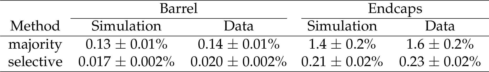
Table 5:
Charge misidentification probability for a tight selection of electrons from ${\mathrm{ Z } } \to \mathrm{ e }^+ \mathrm{ e }^- $ decays in the barrel and in the endcaps, for the majority and for the selective methods used to estimate electron charge. Only statistical uncertainties are shown in the table. |
png pdf |
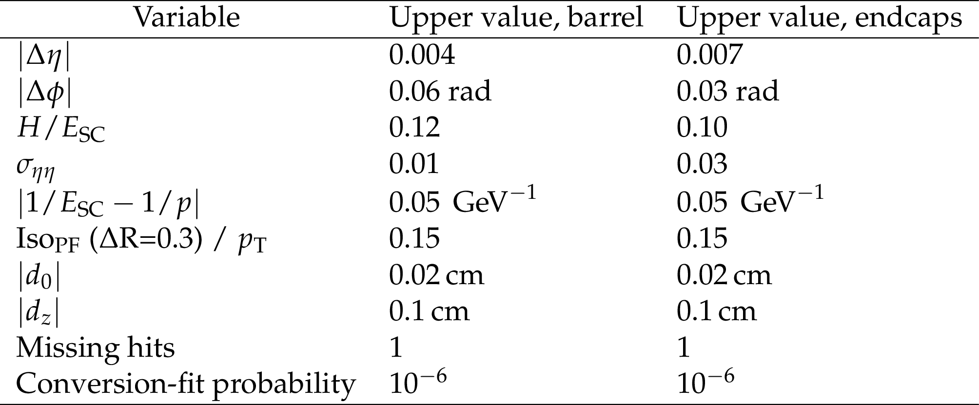
Table 6:
Requirements corresponding to the medium working point of the sequential selection for electrons in the ECAL barrel and endcaps. At most one missing hit is allowed. |
| Summary |
|
The performance of electron reconstruction and selection in CMS has been studied using data collected in proton-proton collisions at $ \sqrt{s} = $ 8 TeV corresponding to an integrated luminosity of 19.7 fb$^{-1}$. Algorithms used to reconstruct electron trajectories and energy deposits in the tracker and ECAL respectively, have been presented. A Gaussian sum filter algorithm used for track reconstruction provides a way to follow the track curvature and to account for bremsstrahlung loss up to the entrance into the ECAL. The strategies for finding seeds for electron tracks, constructing trajectories, and fitting track parameters are optimized to reconstruct the electrons down to small $p_\mathrm{T}$ values with high efficiency and accuracy. Moreover, the clustering of energy in the ECAL and its optimization to recover bremsstrahlung photons are discussed. Dedicated algorithms are used to correct the energy measured in the ECAL as well as to estimate the electron momentum by combining independent measurements in the ECAL and in the tracker. The overall momentum scale is calibrated with an uncertainty smaller than 0.3% in the $p_\mathrm{T}$ range from 7 to 70 GeV. For electrons from Z boson decays, the effective momentum resolution varies from 1.7%, for well-measured electrons with a single-cluster supercluster in the barrel, to 4.5% for electrons with a multi-cluster supercluster, or poorly measured, in the endcaps. The electron momentum resolution is modelled in simulation with a precision better than 10% up to a $p_\mathrm{T}$ of 70 GeV. The performance of the reconstruction algorithms in data is studied together with those of several benchmark selections designed to cover the needs of the physics programme of the CMS experiment. Good agreement is observed between data and predictions from simulation for most of the variables relevant to electron reconstruction and selection. The origin of small remaining discrepancies is understood and corrections will be implemented in the future. The reconstruction efficiency as well as the efficiency of all the selections are measured using $\mathrm{ Z } \to \mathrm{ e }^+\mathrm{ e }^-$ samples in data and in simulation. The reconstruction efficiency in the data ranges from 88% to 98% in the barrel and from 90% to 96% in the endcaps in the $p_\mathrm{T}$ range from 10 to 100 GeV. The ratios of efficiencies of data to simulation, both for reconstruction and for the different proposed selections, are found to be in general compatible with unity within the respective uncertainties, over the full $p_\mathrm{T}$ range, down to a $p_\mathrm{T}$ as low as 7 GeV. Differences of up to 5% between data and simulation are observed in most cases, while differences of up to 15% are measured for a few points at small $p_\mathrm{T}$ values. The analysis of electron performance with data has shown that, despite the challenging conditions of pileup at the LHC and the significant level of bremsstrahlung in the tracker, using dedicated algorithms and a large number of recorded $\mathrm{Z} to \mathrm{ e }^+\mathrm{ e }^-$ decays provided successful means of reconstructing and identifying electrons in CMS. The quality of simulation at the beginning of the experiment was sufficiently good to require only a few adjustments to the originally conceived reconstruction algorithms, and also enabled quick deployment of sophisticated developments, such as PF reconstruction and the use of MVA methods for electron identification and, later, for momentum correction. The reconstruction and selection of electrons at low $p_\mathrm{T}$ have been achieved with a performance level close to that anticipated at the time the detector was designed. These achievements, especially for low-$p_\mathrm{T}$ electrons, played an essential role in the discovery of the Higgs boson at CMS [43,44], and in the measurement of its properties [45] in the $\mathrm{ H \to ZZ* \to 4 \ell }$ channel. |
| References | ||||
| 1 | CMS Collaboration | CMS: The TriDAS project. Technical design report, Vol.2: Data acquisition and high-level trigger | link | |
| 2 | CMS Collaboration | CMS physics: Technical design report volume 1: Detector performance | link | |
| 3 | S. Baffioni et al. | Electron reconstruction in CMS | EPJC 49 (2007) 1099 | |
| 4 | CMS Collaboration | Energy calibration and resolution of the CMS electromagnetic calorimeter in pp collisions at $ \sqrt{s} $ = 7 TeV | JINST 8 (2013) P09009 | CMS-EGM-11-001 1306.2016 |
| 5 | CMS Collaboration | Description and performance of track and primary vertex reconstruction with the CMS tracker | JINST 9 (2014) P10009 | CMS-TRK-11-001 1405.6569 |
| 6 | CMS Collaboration | Electron Reconstruction and Identification at $ \sqrt{s} = 7 $ TeV | CDS | |
| 7 | CMS Collaboration | Electron commissioning results at $ \sqrt{s} $ = 7 TeV | link | |
| 8 | CMS Collaboration | Electron performance with 19.6 fb$ ^{-1} $ of data collected at $ \sqrt{s} $ = 8 TeV with the CMS detector | link | |
| 9 | CMS Collaboration | Measurement of the properties of a Higgs boson in the four-lepton final state | PRD 89 (2014) 092007 | hep-ex/1312.5353 |
| 10 | CMS Collaboration | Search for heavy narrow dilepton resonances in pp collisions at $ \sqrt{s}=7 $ TeV and $ \sqrt{s}=8 $ TeV | PLB 720 (2013) 63 | CMS-EXO-12-015 1212.6175 |
| 11 | CMS Collaboration | The CMS experiment at the CERN LHC | JINST 3 (2008) S08004 | CMS-00-001 |
| 12 | CMS Collaboration | CMS Luminosity Based on Pixel Cluster Counting - Summer 2013 Update | CDS | CMS-PAS-LUM-13-001 |
| 13 | CMS Collaboration | Alignment of the CMS tracker with LHC and cosmic ray data | JINST 9 (2014) P06009 | CMS-TRK-11-002 1403.2286 |
| 14 | J. Alwall et al. | The automated computation of tree-level and next-to-leading order differential cross sections, and their matching to parton shower simulations | JHEP 07 (2014) 079 | 1405.0301 |
| 15 | P. Nason | A New method for combining NLO QCD with shower Monte Carlo algorithms | JHEP 11 (2004) 040 | hep-ph/0409146 |
| 16 | S. Frixione, P. Nason, and C. Oleari | Matching NLO QCD computations with parton shower simulations: the POWHEG method | JHEP 11 (2007) 070 | 0709.2092 |
| 17 | S. Alioli, P. Nason, C. Oleari, and E. Re | A general framework for implementing NLO calculations in shower Monte Carlo programs: the POWHEG BOX | JHEP 06 (2010) 043 | 1002.2581 |
| 18 | T. Sjostrand, S. Mrenna, and P. Z. Skands | PYTHIA 6.4 physics and manual | JHEP 05 (2006) 026 | hep-ph/0603175 |
| 19 | CMS Collaboration | Study of the underlying event at foward rapidity in pp collisions at $ \sqrt{s} $ = 0.9, 2.76, and 7 TeV | JHEP 04 (2013) 072 | 1302.2394v2 |
| 20 | GEANT4 Collaboration | GEANT4---a simulation toolkit | NIMA 506 (2003) 250 | |
| 21 | J. Allison et al. | GEANT4 developments and applications | IEEE Trans. Nucl. Sci. 53 (2006) 270 | |
| 22 | CMS Collaboration | Particle--Flow Event Reconstruction in CMS and Performance for Jets, Taus, and \MET | CDS | |
| 23 | CMS Collaboration | Commissioning of the Particle-flow Event Reconstruction with the first LHC collisions recorded in the CMS detector | CDS | |
| 24 | P. Adzic et al. | Energy resolution of the barrel of the CMS Electromagnetic Calorimeter | JINST 2 (2007) P04004 | |
| 25 | W. Adam, R. Fruhwirth, A. Strandlie, and T. Todorov | Reconstruction of electrons with the Gaussian-sum filter in the CMS tracker at LHC | JPG 31 (2005) N9 | |
| 26 | H. Voss, A. Hocker, J. Stelzer, and F. Tegenfeldt | TMVA, the Toolkit for Multivariate Data Analysis with ROOT | link | physics/0703039 |
| 27 | CMS Collaboration | Performance of photon reconstruction and identification with the CMS detector in proton-proton collisions at $ \sqrt{s}= $ 8 TeV | JINST 10 (2015) P08010 | CMS-EGM-14-001 1502.02702 |
| 28 | CMS Collaboration | Measurement of the electron charge asymmetry in inclusive $ W $ production in pp collisions at $ \sqrt{s} $ = 7 TeV | PRL 109 (2012) 111806 | CMS-SMP-12-001 1206.2598 |
| 29 | CMS Collaboration | Search for new physics in events with same-sign dileptons and jets in pp collisions at $ \sqrt{s} $ = 8 TeV | JHEP 01 (2014) 163 | CMS-SUS-13-013 1311.6736 |
| 30 | M. Anfreville et al. | Laser monitoring system for the CMS lead tungstate crystal calorimeter | NIMA 594 (2008) 292 | |
| 31 | L.-Y. Zhang et al. | Performance of the monitoring light source for the CMS lead tungstate crystal calorimeter | IEEE Trans. Nucl. Sci. 52 (2005) 1123 | |
| 32 | J. H. Friedman | Greedy function approximation: A gradient boosting machine | Ann. of Stat. 29 (2001) 1189 | |
| 33 | S. Catani, Y. L. Dokshitzer, M. H. Seymour, and B. R. Webber | Longitudinally invariant $ k_{\perp} $ clustering algorithms for hadron-hadron collisions | Nucl. Phys. B 406 (1993) 187 | |
| 34 | S. D. Ellis and D. E. Soper | Successive combination jet algorithm for hadron collisions | PRD 48 (1993) 3160 | hep-ph/9305266 |
| 35 | M. Oreglia | A study of the reactions $\psi^\prime \to \gamma \gamma \psi$ | PhD thesis, Stanford University, 1980. SLAC-R-236 | |
| 36 | Particle Data Group, K. A. Olive et al. | The Review of Particle Physics | CPC 38 (2014) 090001 | |
| 37 | GEANT4 Collaboration | GEANT4 10.0 Release Notes | link | |
| 38 | M. Pivk and F. R. Le Diberder | sPlot: a statistical tool to unfold data distributions | NIMA 555 (2005) 356 | physics/0402083 |
| 39 | M. Cacciari and G. P. Salam | Pileup subtraction using jet areas | PLB 659 (2008) 119 | 0707.1378 |
| 40 | M. Cacciari, G. P. Salam, and G. Soyez | The catchment area of jets | JHEP 04 (2008) 005 | 0802.1188 |
| 41 | M. Cacciari, G. P. Salam, and G. Soyez | FastJet user manual | EPJC 72 (2012) 1896 | 1111.6097 |
| 42 | CMS Collaboration | Measurements of Inclusive W and Z Cross Sections in pp Collisions at $ \sqrt{s} $ = 7 TeV | JHEP 01 (2011) 080 | CMS-EWK-10-002 1012.2466 |
| 43 | CMS Collaboration | Observation of a new boson at a mass of 125 GeV with the CMS experiment at the LHC | PLB 716 (2012) 30 | |
| 44 | CMS Collaboration | Observation of a new boson with mass near 125 GeV in pp collisions at $ \sqrt{s} $ = 7 and 8 TeV | JHEP 06 (2013) 081 | CMS-HIG-12-036 1303.4571 |
| 45 | CMS Collaboration | Precise determination of the mass of the Higgs boson and tests of compatibility of its couplings with the standard model predictions using proton collisions at 7 and 8 TeV | CMS-HIG-14-009 1412.8662 |
|
|
|
Compact Muon Solenoid LHC, CERN |
|

|

|

|

|

|