

Compact Muon Solenoid
LHC, CERN
| CMS-MUO-10-004 ; CERN-PH-EP-2012-173 | ||
| Performance of CMS muon reconstruction in pp collision events at $\sqrt{s} = $ 7 TeV | ||
| CMS Collaboration | ||
| 19 June 2012 | ||
| J. Instrum. 7 (2012) P10002 | ||
| Abstract: The performance of muon reconstruction, identification, and triggering in CMS has been studied using 40 pb$^{-1}$ of data collected in pp collisions at $\sqrt{s} = $ 7 TeV at the LHC in 2010. A few benchmark sets of selection criteria covering a wide range of physics analysis needs have been examined. For all considered selections, the efficiency to reconstruct and identify a muon with a transverse momentum $p_{\mathrm{T}}$ larger than a few GeVc is above 95% over the whole region of pseudorapidity covered by the CMS muon system, $|\eta|< $ 2.4, while the probability to misidentify a hadron as a muon is well below 1%. The efficiency to trigger on single muons with $p_{\mathrm{T}}$ above a few GeVc is higher than 90% over the full $\eta$ range, and typically substantially better. The overall momentum scale is measured to a precision of 0.2% with muons from Z decays. The transverse momentum resolution varies from 1% to 6% depending on pseudorapidity for muons with $p_{\mathrm{T}}$ below 100 GeV/$c$ and, using cosmic rays, it is shown to be better than 10% in the central region up to $p_{\mathrm{T}} = $ 1 TeV/$c$. Observed distributions of all quantities are well reproduced by the Monte Carlo simulation. | ||
| Links: e-print arXiv:1206.4071 [physics.ins-det] (PDF) ; CDS record ; inSPIRE record ; CADI line (restricted) ; | ||
| Figures | |

png pdf |
Figure 1:
Longitudinal layout of one quadrant of the CMS detector. The four DT stations in the barrel (MB1-MB4, green), the four CSC stations in the endcap (ME1-ME4, blue), and the RPC stations (red) are shown. |

png pdf |
Figure 2:
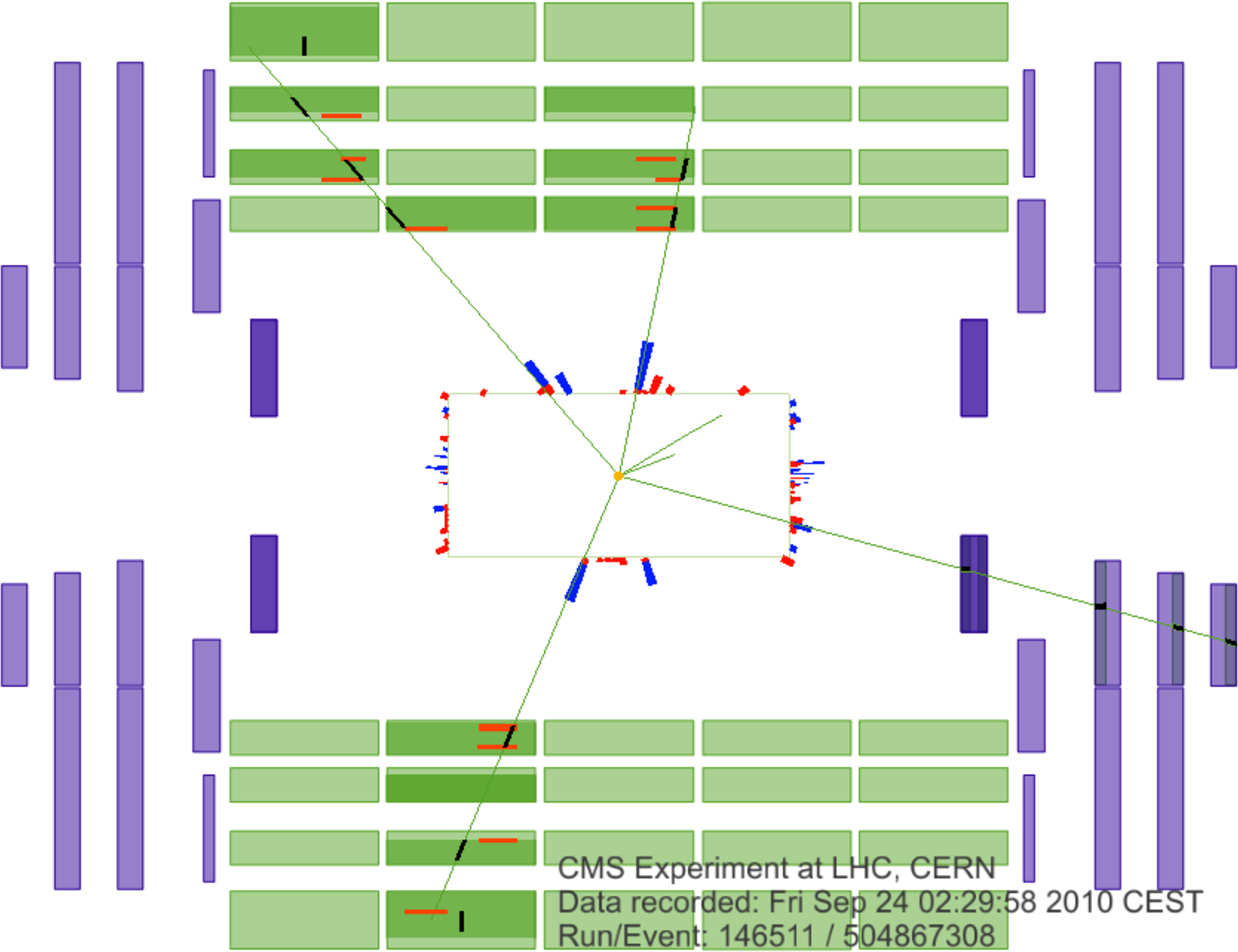
(a) The longitudinal ($r$-$z$) and b) the transverse ($r$-$\phi $) views of a collision event in which four muons were reconstructed. The green (thin) curves in the inner cylinder represent tracks of charged particles reconstructed in the inner tracker with transverse momentum $ {p_{\mathrm {T}}} > $ 1 GeV/$c$; those extending to the muon system represent tracks of muons reconstructed using hits in both inner tracker and the muon system. Three muons were identified by the DTs and RPCs, the fourth one by the CSCs. Short black stubs in the muon system show fitted muon-track segments; as the $z$ position is not measured in the outer barrel station, the segments in it are drawn at the $z$ centre of the wheel, with their directions perpendicular to the chamber. Short red (light) horizontal lines in the $r$-$z$ view indicate positions of RPC hits; energy depositions in the ECAL and HCAL are shown as red (light) and blue (dark) bars, respectively. |
png pdf |
Figure 2-a:
(a) The longitudinal ($r$-$z$) and b) the transverse ($r$-$\phi $) views of a collision event in which four muons were reconstructed. The green (thin) curves in the inner cylinder represent tracks of charged particles reconstructed in the inner tracker with transverse momentum $ {p_{\mathrm {T}}} > $ 1 GeV/$c$; those extending to the muon system represent tracks of muons reconstructed using hits in both inner tracker and the muon system. Three muons were identified by the DTs and RPCs, the fourth one by the CSCs. Short black stubs in the muon system show fitted muon-track segments; as the $z$ position is not measured in the outer barrel station, the segments in it are drawn at the $z$ centre of the wheel, with their directions perpendicular to the chamber. Short red (light) horizontal lines in the $r$-$z$ view indicate positions of RPC hits; energy depositions in the ECAL and HCAL are shown as red (light) and blue (dark) bars, respectively. |

png pdf |
Figure 2-b:
(a) The longitudinal ($r$-$z$) and b) the transverse ($r$-$\phi $) views of a collision event in which four muons were reconstructed. The green (thin) curves in the inner cylinder represent tracks of charged particles reconstructed in the inner tracker with transverse momentum $ {p_{\mathrm {T}}} > $ 1 GeV/$c$; those extending to the muon system represent tracks of muons reconstructed using hits in both inner tracker and the muon system. Three muons were identified by the DTs and RPCs, the fourth one by the CSCs. Short black stubs in the muon system show fitted muon-track segments; as the $z$ position is not measured in the outer barrel station, the segments in it are drawn at the $z$ centre of the wheel, with their directions perpendicular to the chamber. Short red (light) horizontal lines in the $r$-$z$ view indicate positions of RPC hits; energy depositions in the ECAL and HCAL are shown as red (light) and blue (dark) bars, respectively. |
png pdf |
Figure 3:
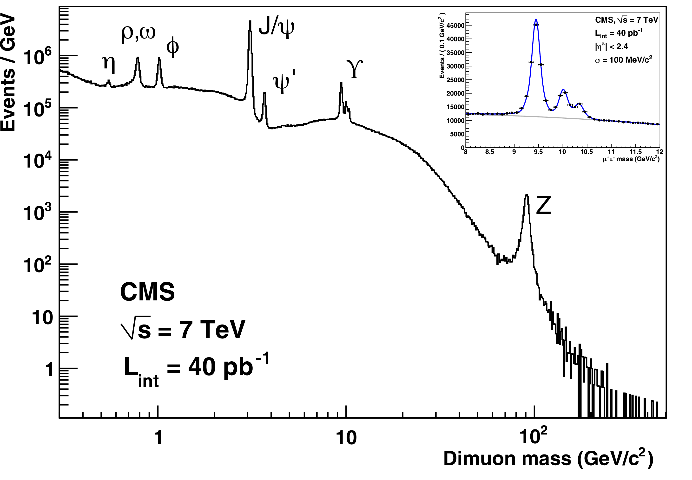
Invariant mass spectrum of dimuons in events collected with the loose double-muon trigger in 2010. The inset is a zoom of the 8-12 GeV/$c^2$ region, showing the three $\Upsilon (nS)$ peaks clearly resolved owing to a good mass resolution, about 100 MeV/$c^2$ in the entire pseudorapidity range and 70 MeV/$c^2$ when both muons are within the range $|\eta | < 1$. |
png pdf |
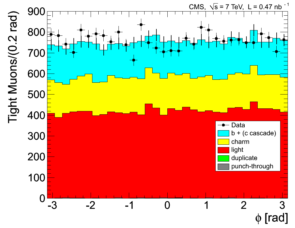
Figure 4:
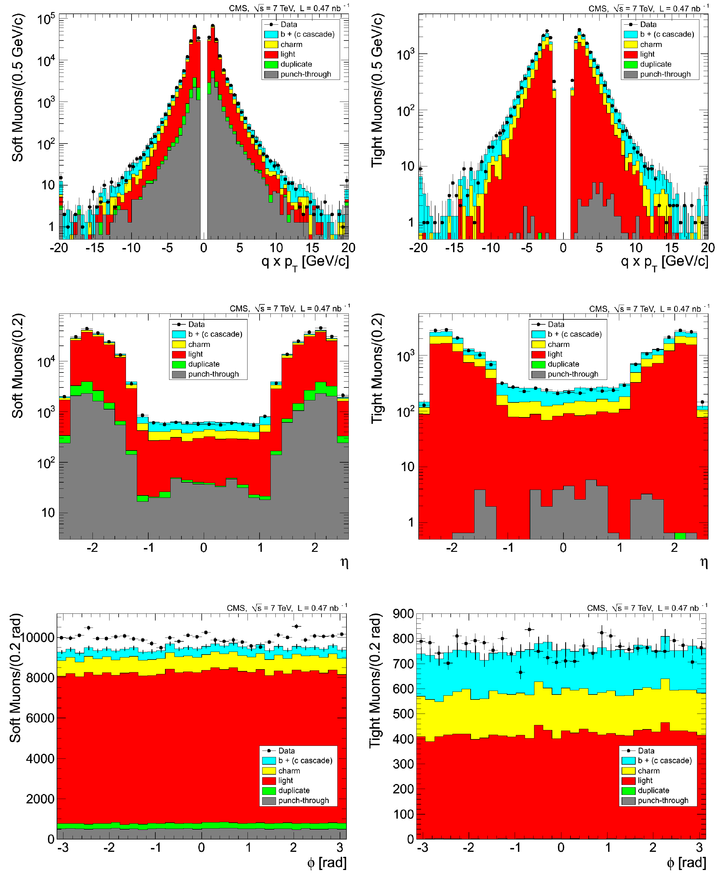
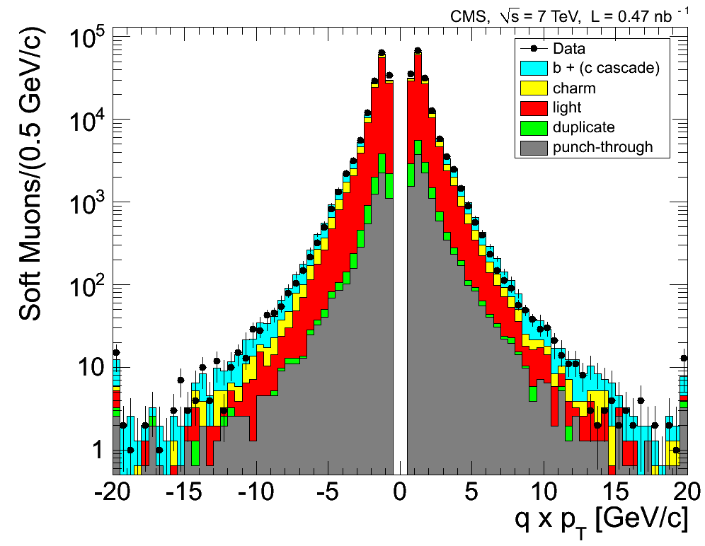
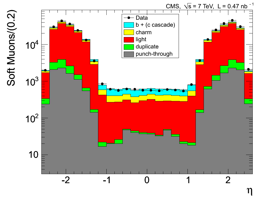
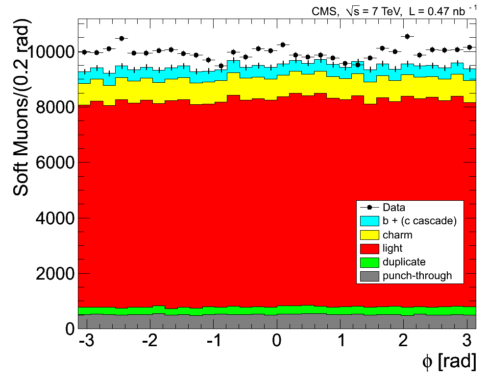
Distributions of kinematic variables for a sample of muons selected by the zero-bias trigger, for data (points) and for simulation subdivided into the different categories of contributing muons (histograms). The kinematic variables are the muon transverse momentum multiplied by the charge (top), pseudorapidity (middle), and azimuthal angle (bottom). For each variable, the left plot shows the distribution for Soft Muons, and the right plot that for Tight Muons. The first (last) bin in the $q \times {p_{\mathrm {T}}} $ distributions includes the underflow (the overflow). The error bars indicate the statistical uncertainty, for both data and MC samples. |
png |
Figure 4-a:
Distributions of kinematic variables for a sample of muons selected by the zero-bias trigger, for data (points) and for simulation subdivided into the different categories of contributing muons (histograms). The kinematic variables are the muon transverse momentum multiplied by the charge (top), pseudorapidity (middle), and azimuthal angle (bottom). For each variable, the left plot shows the distribution for Soft Muons, and the right plot that for Tight Muons. The first (last) bin in the $q \times {p_{\mathrm {T}}} $ distributions includes the underflow (the overflow). The error bars indicate the statistical uncertainty, for both data and MC samples. |
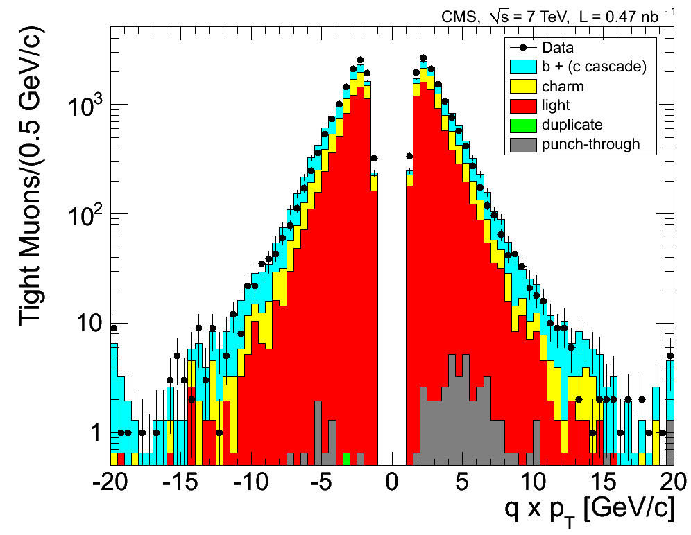
png |
Figure 4-b:
Distributions of kinematic variables for a sample of muons selected by the zero-bias trigger, for data (points) and for simulation subdivided into the different categories of contributing muons (histograms). The kinematic variables are the muon transverse momentum multiplied by the charge (top), pseudorapidity (middle), and azimuthal angle (bottom). For each variable, the left plot shows the distribution for Soft Muons, and the right plot that for Tight Muons. The first (last) bin in the $q \times {p_{\mathrm {T}}} $ distributions includes the underflow (the overflow). The error bars indicate the statistical uncertainty, for both data and MC samples. |
png |
Figure 4-c:
Distributions of kinematic variables for a sample of muons selected by the zero-bias trigger, for data (points) and for simulation subdivided into the different categories of contributing muons (histograms). The kinematic variables are the muon transverse momentum multiplied by the charge (top), pseudorapidity (middle), and azimuthal angle (bottom). For each variable, the left plot shows the distribution for Soft Muons, and the right plot that for Tight Muons. The first (last) bin in the $q \times {p_{\mathrm {T}}} $ distributions includes the underflow (the overflow). The error bars indicate the statistical uncertainty, for both data and MC samples. |
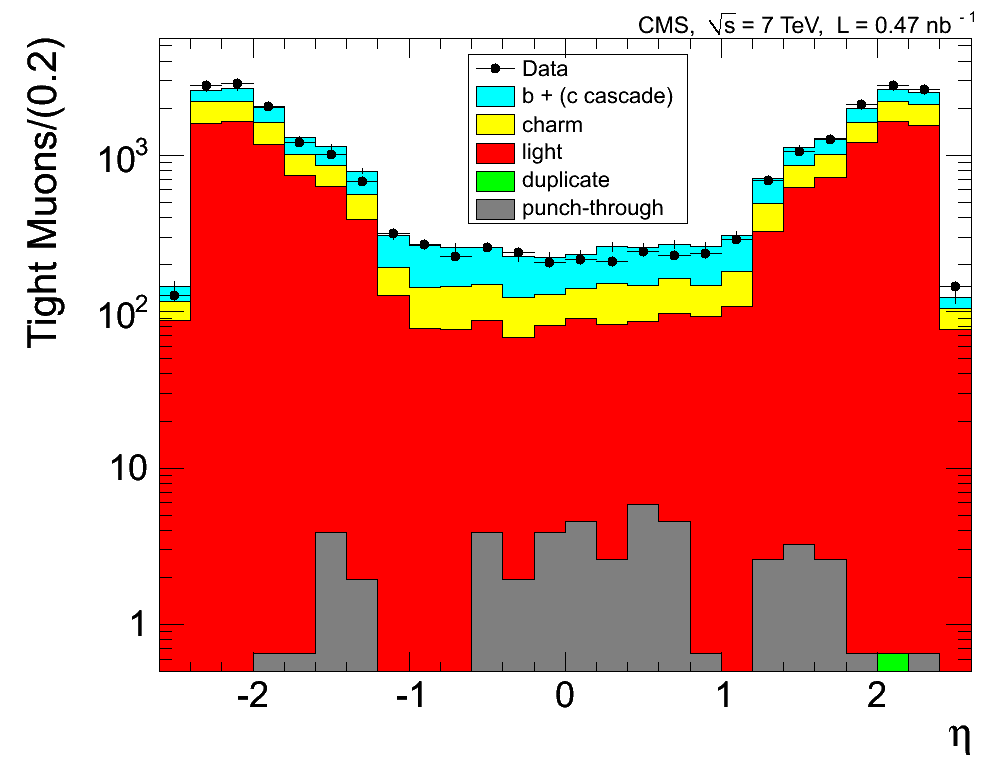
png |
Figure 4-d:
Distributions of kinematic variables for a sample of muons selected by the zero-bias trigger, for data (points) and for simulation subdivided into the different categories of contributing muons (histograms). The kinematic variables are the muon transverse momentum multiplied by the charge (top), pseudorapidity (middle), and azimuthal angle (bottom). For each variable, the left plot shows the distribution for Soft Muons, and the right plot that for Tight Muons. The first (last) bin in the $q \times {p_{\mathrm {T}}} $ distributions includes the underflow (the overflow). The error bars indicate the statistical uncertainty, for both data and MC samples. |
png |
Figure 4-e:
Distributions of kinematic variables for a sample of muons selected by the zero-bias trigger, for data (points) and for simulation subdivided into the different categories of contributing muons (histograms). The kinematic variables are the muon transverse momentum multiplied by the charge (top), pseudorapidity (middle), and azimuthal angle (bottom). For each variable, the left plot shows the distribution for Soft Muons, and the right plot that for Tight Muons. The first (last) bin in the $q \times {p_{\mathrm {T}}} $ distributions includes the underflow (the overflow). The error bars indicate the statistical uncertainty, for both data and MC samples. |
png |
Figure 4-f:
Distributions of kinematic variables for a sample of muons selected by the zero-bias trigger, for data (points) and for simulation subdivided into the different categories of contributing muons (histograms). The kinematic variables are the muon transverse momentum multiplied by the charge (top), pseudorapidity (middle), and azimuthal angle (bottom). For each variable, the left plot shows the distribution for Soft Muons, and the right plot that for Tight Muons. The first (last) bin in the $q \times {p_{\mathrm {T}}} $ distributions includes the underflow (the overflow). The error bars indicate the statistical uncertainty, for both data and MC samples. |

png pdf |
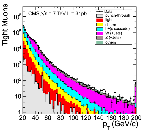
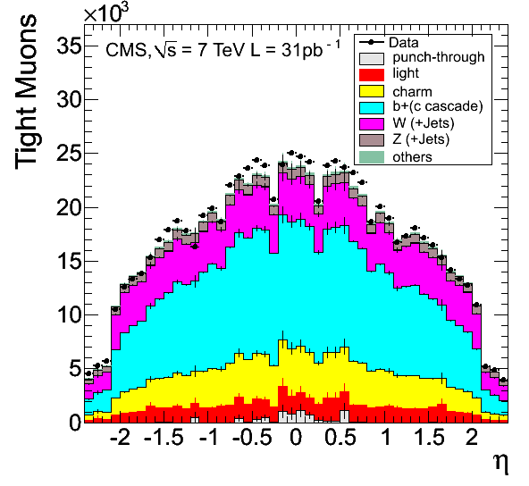
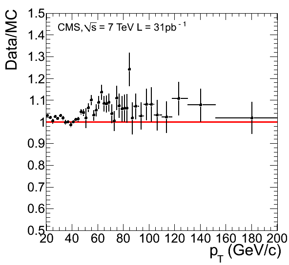
Figure 5:
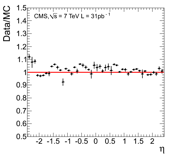
Distributions of transverse momentum (top left) and pseudorapidity (top right) for Tight Muons with $ {p_{\mathrm {T}}} > $ 20 GeV/$c$, comparing data (points with error bars) to Monte Carlo simulation broken down into its different components. The last bin in the $ {p_{\mathrm {T}}} $ distribution includes the overflow. Dips in the $\eta $ distribution are due to inefficiencies related to the muon detector geometry. The corresponding ratios of data and MC distributions are shown in the bottom row. The error bars include statistical uncertainties only. |
png |
Figure 5-a:
Distributions of transverse momentum (top left) and pseudorapidity (top right) for Tight Muons with $ {p_{\mathrm {T}}} > $ 20 GeV/$c$, comparing data (points with error bars) to Monte Carlo simulation broken down into its different components. The last bin in the $ {p_{\mathrm {T}}} $ distribution includes the overflow. Dips in the $\eta $ distribution are due to inefficiencies related to the muon detector geometry. The corresponding ratios of data and MC distributions are shown in the bottom row. The error bars include statistical uncertainties only. |
png |
Figure 5-b:
Distributions of transverse momentum (top left) and pseudorapidity (top right) for Tight Muons with $ {p_{\mathrm {T}}} > $ 20 GeV/$c$, comparing data (points with error bars) to Monte Carlo simulation broken down into its different components. The last bin in the $ {p_{\mathrm {T}}} $ distribution includes the overflow. Dips in the $\eta $ distribution are due to inefficiencies related to the muon detector geometry. The corresponding ratios of data and MC distributions are shown in the bottom row. The error bars include statistical uncertainties only. |
png |
Figure 5-c:
Distributions of transverse momentum (top left) and pseudorapidity (top right) for Tight Muons with $ {p_{\mathrm {T}}} > $ 20 GeV/$c$, comparing data (points with error bars) to Monte Carlo simulation broken down into its different components. The last bin in the $ {p_{\mathrm {T}}} $ distribution includes the overflow. Dips in the $\eta $ distribution are due to inefficiencies related to the muon detector geometry. The corresponding ratios of data and MC distributions are shown in the bottom row. The error bars include statistical uncertainties only. |
png |
Figure 5-d:
Distributions of transverse momentum (top left) and pseudorapidity (top right) for Tight Muons with $ {p_{\mathrm {T}}} > $ 20 GeV/$c$, comparing data (points with error bars) to Monte Carlo simulation broken down into its different components. The last bin in the $ {p_{\mathrm {T}}} $ distribution includes the overflow. Dips in the $\eta $ distribution are due to inefficiencies related to the muon detector geometry. The corresponding ratios of data and MC distributions are shown in the bottom row. The error bars include statistical uncertainties only. |
png pdf |
Figure 6:
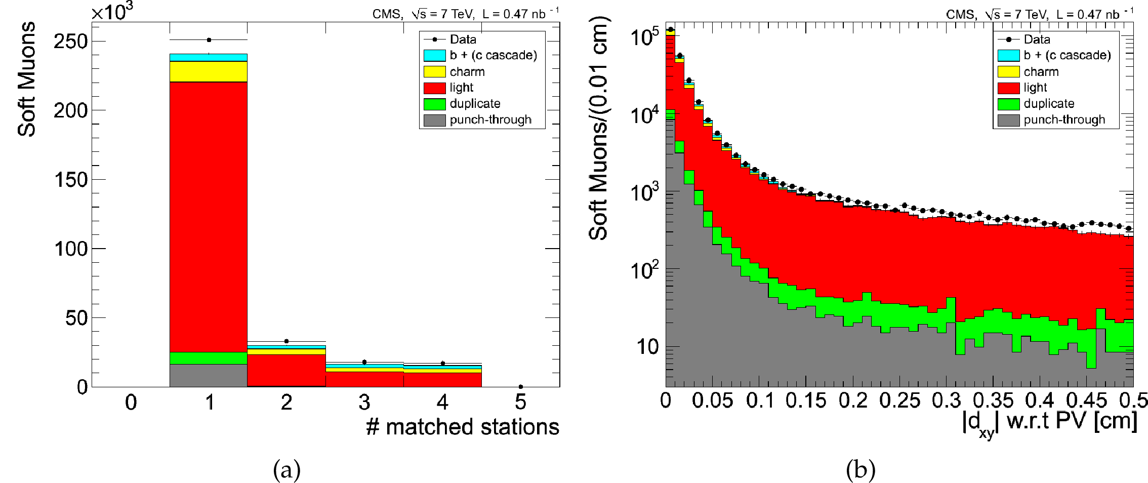
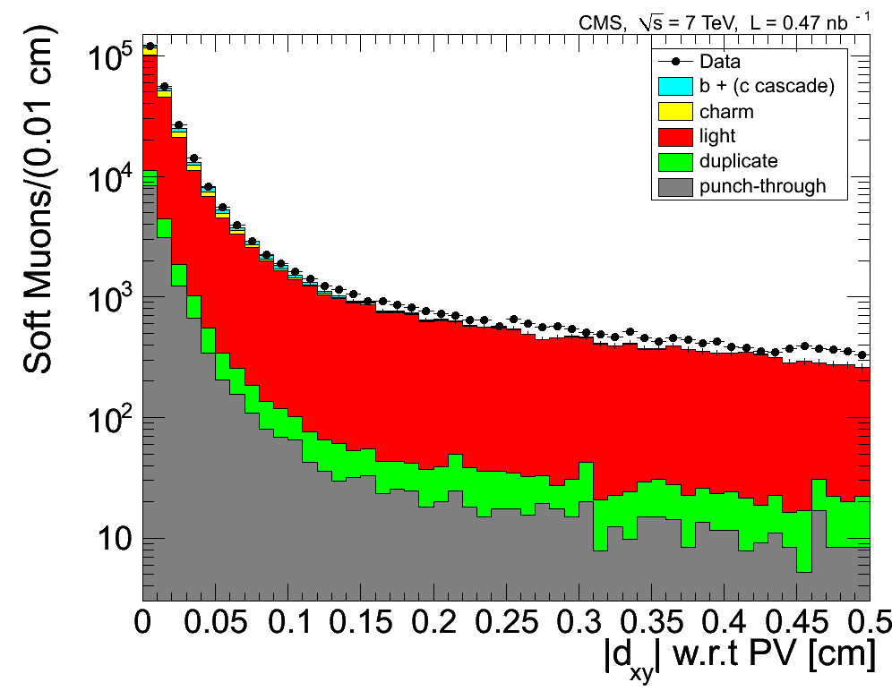
Comparison of data and simulation for distributions of Soft Muons in zero-bias events: (a) number of muon stations with matched segments; (b) transverse impact parameter $d_{\rm xy}$ of the muon with respect to the primary vertex (PV). The MC distributions are normalized to the integrated luminosity of the data sample. The error bars indicate the statistical uncertainty. |

png |
Figure 6-a:
Comparison of data and simulation for distributions of Soft Muons in zero-bias events: (a) number of muon stations with matched segments; (b) transverse impact parameter $d_{\rm xy}$ of the muon with respect to the primary vertex (PV). The MC distributions are normalized to the integrated luminosity of the data sample. The error bars indicate the statistical uncertainty. |
png |
Figure 6-b:
Comparison of data and simulation for distributions of Soft Muons in zero-bias events: (a) number of muon stations with matched segments; (b) transverse impact parameter $d_{\rm xy}$ of the muon with respect to the primary vertex (PV). The MC distributions are normalized to the integrated luminosity of the data sample. The error bars indicate the statistical uncertainty. |

png pdf |
Figure 7:
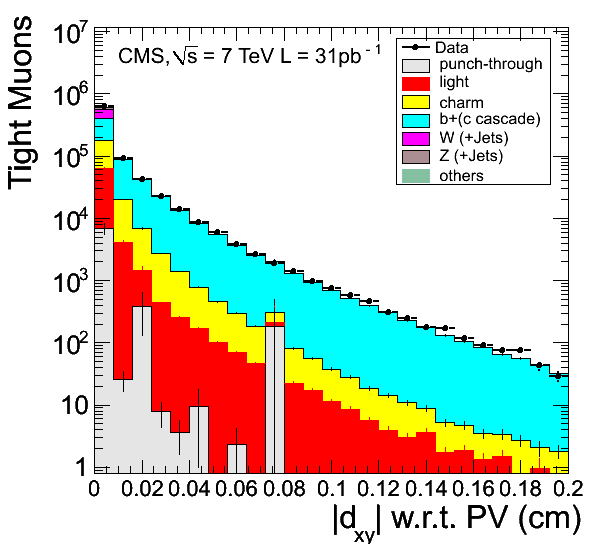
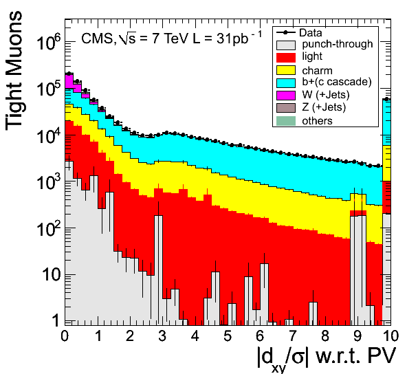
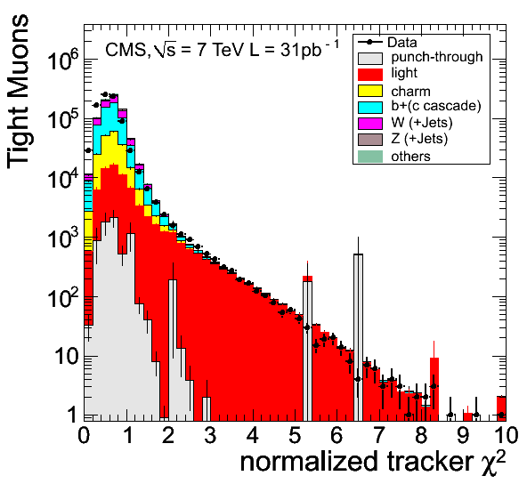
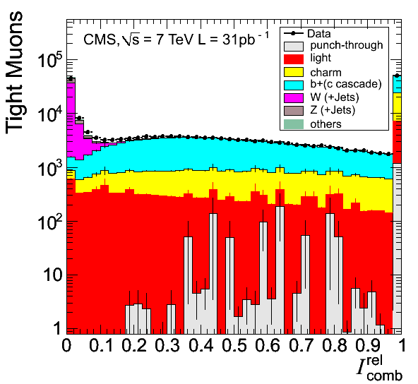
Identification variables for Tight Muons with $ {p_{\mathrm {T}}} > $ 20 GeV/$c$: (a) transverse impact parameter $d_{\rm xy}$ with respect to the primary vertex (PV); (b) significance of the transverse impact parameter; (c) $\chi ^2/d.o.f.$ of the fit of the track in the inner tracker; (d) relative combined isolation (tracker+calorimeters), with a cone size $\Delta R=0.3$, for events with a single reconstructed PV. The MC distributions are normalized to the integrated luminosity of the data sample in (a), (b), and (c), and to the number of events in the data sample in (d). The last bin in (b) and in (d) includes the overflow. Error bars indicate statistical uncertainties. |
png |
Figure 7-a:
Identification variables for Tight Muons with $ {p_{\mathrm {T}}} > $ 20 GeV/$c$: (a) transverse impact parameter $d_{\rm xy}$ with respect to the primary vertex (PV); (b) significance of the transverse impact parameter; (c) $\chi ^2/d.o.f.$ of the fit of the track in the inner tracker; (d) relative combined isolation (tracker+calorimeters), with a cone size $\Delta R=0.3$, for events with a single reconstructed PV. The MC distributions are normalized to the integrated luminosity of the data sample in (a), (b), and (c), and to the number of events in the data sample in (d). The last bin in (b) and in (d) includes the overflow. Error bars indicate statistical uncertainties. |
png |
Figure 7-b:
Identification variables for Tight Muons with $ {p_{\mathrm {T}}} > $ 20 GeV/$c$: (a) transverse impact parameter $d_{\rm xy}$ with respect to the primary vertex (PV); (b) significance of the transverse impact parameter; (c) $\chi ^2/d.o.f.$ of the fit of the track in the inner tracker; (d) relative combined isolation (tracker+calorimeters), with a cone size $\Delta R=0.3$, for events with a single reconstructed PV. The MC distributions are normalized to the integrated luminosity of the data sample in (a), (b), and (c), and to the number of events in the data sample in (d). The last bin in (b) and in (d) includes the overflow. Error bars indicate statistical uncertainties. |
png |
Figure 7-c:
Identification variables for Tight Muons with $ {p_{\mathrm {T}}} > $ 20 GeV/$c$: (a) transverse impact parameter $d_{\rm xy}$ with respect to the primary vertex (PV); (b) significance of the transverse impact parameter; (c) $\chi ^2/d.o.f.$ of the fit of the track in the inner tracker; (d) relative combined isolation (tracker+calorimeters), with a cone size $\Delta R=0.3$, for events with a single reconstructed PV. The MC distributions are normalized to the integrated luminosity of the data sample in (a), (b), and (c), and to the number of events in the data sample in (d). The last bin in (b) and in (d) includes the overflow. Error bars indicate statistical uncertainties. |
png |
Figure 7-d:
Identification variables for Tight Muons with $ {p_{\mathrm {T}}} > $ 20 GeV/$c$: (a) transverse impact parameter $d_{\rm xy}$ with respect to the primary vertex (PV); (b) significance of the transverse impact parameter; (c) $\chi ^2/d.o.f.$ of the fit of the track in the inner tracker; (d) relative combined isolation (tracker+calorimeters), with a cone size $\Delta R=0.3$, for events with a single reconstructed PV. The MC distributions are normalized to the integrated luminosity of the data sample in (a), (b), and (c), and to the number of events in the data sample in (d). The last bin in (b) and in (d) includes the overflow. Error bars indicate statistical uncertainties. |
png pdf |
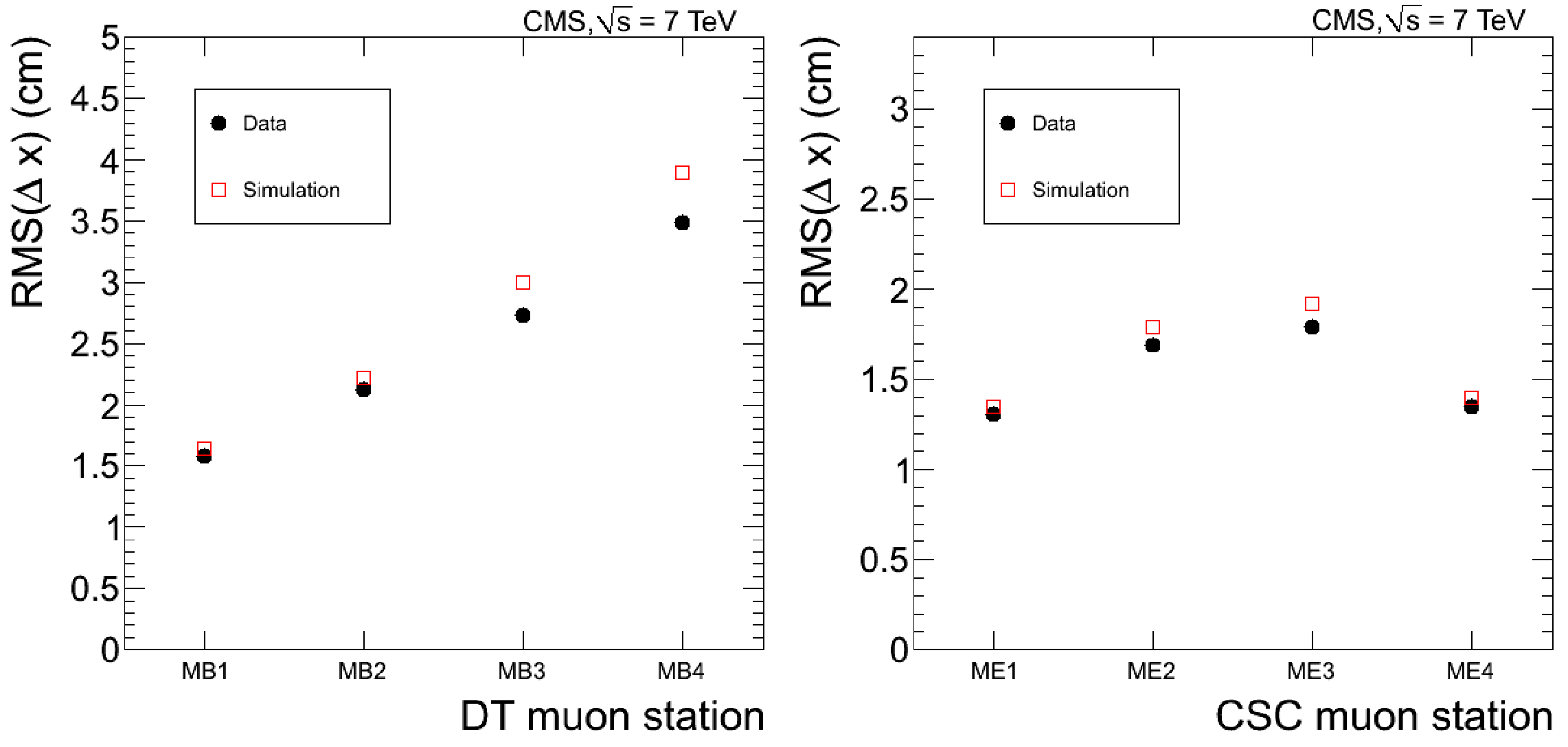
Figure 8:
RMS width of residuals of the local $x$ position, given by the position of the muon segment with respect to the extrapolated tracker track, as a function of the muon station, for DT chambers in the barrel region (left) and CSCs in the endcap regions (right). Data are compared with MC expectations. |
png |
Figure 8-a:
RMS width of residuals of the local $x$ position, given by the position of the muon segment with respect to the extrapolated tracker track, as a function of the muon station, for DT chambers in the barrel region (left) and CSCs in the endcap regions (right). Data are compared with MC expectations. |

png |
Figure 8-b:
RMS width of residuals of the local $x$ position, given by the position of the muon segment with respect to the extrapolated tracker track, as a function of the muon station, for DT chambers in the barrel region (left) and CSCs in the endcap regions (right). Data are compared with MC expectations. |

png pdf |
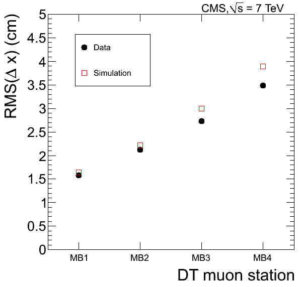
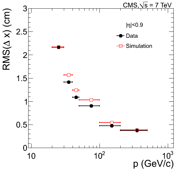
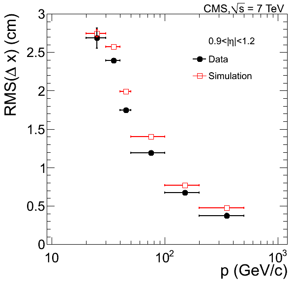
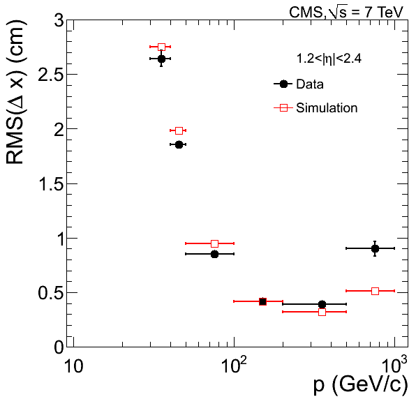
Figure 9:
RMS width of residuals of the local $x$ position for the track-to-segment match in the first muon station (a) as a function of the muon pseudorapidity, with a requirement on momentum $p > $ 90 GeV/$c$, and (b)-(d) as a function of the muon momentum in different angular regions: (b) $|\eta |<0.9$; (c) $0.9<|\eta |<1.2$; (d) $1.2<|\eta |<2.4$. Data are compared with MC expectations. |

png |
Figure 9-a:
RMS width of residuals of the local $x$ position for the track-to-segment match in the first muon station (a) as a function of the muon pseudorapidity, with a requirement on momentum $p > $ 90 GeV/$c$, and (b)-(d) as a function of the muon momentum in different angular regions: (b) $|\eta |<0.9$; (c) $0.9<|\eta |<1.2$; (d) $1.2<|\eta |<2.4$. Data are compared with MC expectations. |
png |
Figure 9-b:
RMS width of residuals of the local $x$ position for the track-to-segment match in the first muon station (a) as a function of the muon pseudorapidity, with a requirement on momentum $p > $ 90 GeV/$c$, and (b)-(d) as a function of the muon momentum in different angular regions: (b) $|\eta |<0.9$; (c) $0.9<|\eta |<1.2$; (d) $1.2<|\eta |<2.4$. Data are compared with MC expectations. |
png |
Figure 9-c:
RMS width of residuals of the local $x$ position for the track-to-segment match in the first muon station (a) as a function of the muon pseudorapidity, with a requirement on momentum $p > $ 90 GeV/$c$, and (b)-(d) as a function of the muon momentum in different angular regions: (b) $|\eta |<0.9$; (c) $0.9<|\eta |<1.2$; (d) $1.2<|\eta |<2.4$. Data are compared with MC expectations. |
png |
Figure 9-d:
RMS width of residuals of the local $x$ position for the track-to-segment match in the first muon station (a) as a function of the muon pseudorapidity, with a requirement on momentum $p > $ 90 GeV/$c$, and (b)-(d) as a function of the muon momentum in different angular regions: (b) $|\eta |<0.9$; (c) $0.9<|\eta |<1.2$; (d) $1.2<|\eta |<2.4$. Data are compared with MC expectations. |
png pdf |
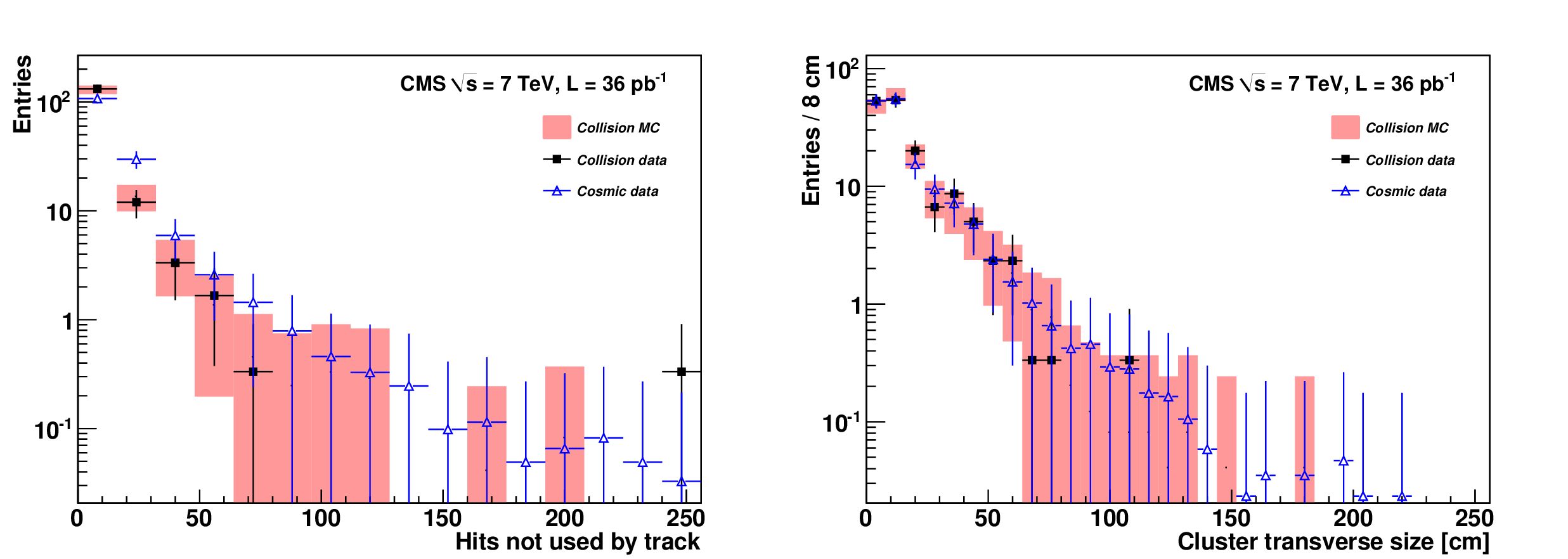
Figure 10:
Comparison of data and simulation for variables characterizing electromagnetic showers, for muons with $p >$ 150 GeV/$c$ in the barrel region: the number of reconstructed muon hits not used in a track fit (left); the transverse size of the cluster of hits around a track (right). All distributions are normalized to the number of muons per muon station in the collision data sample. |
png pdf |
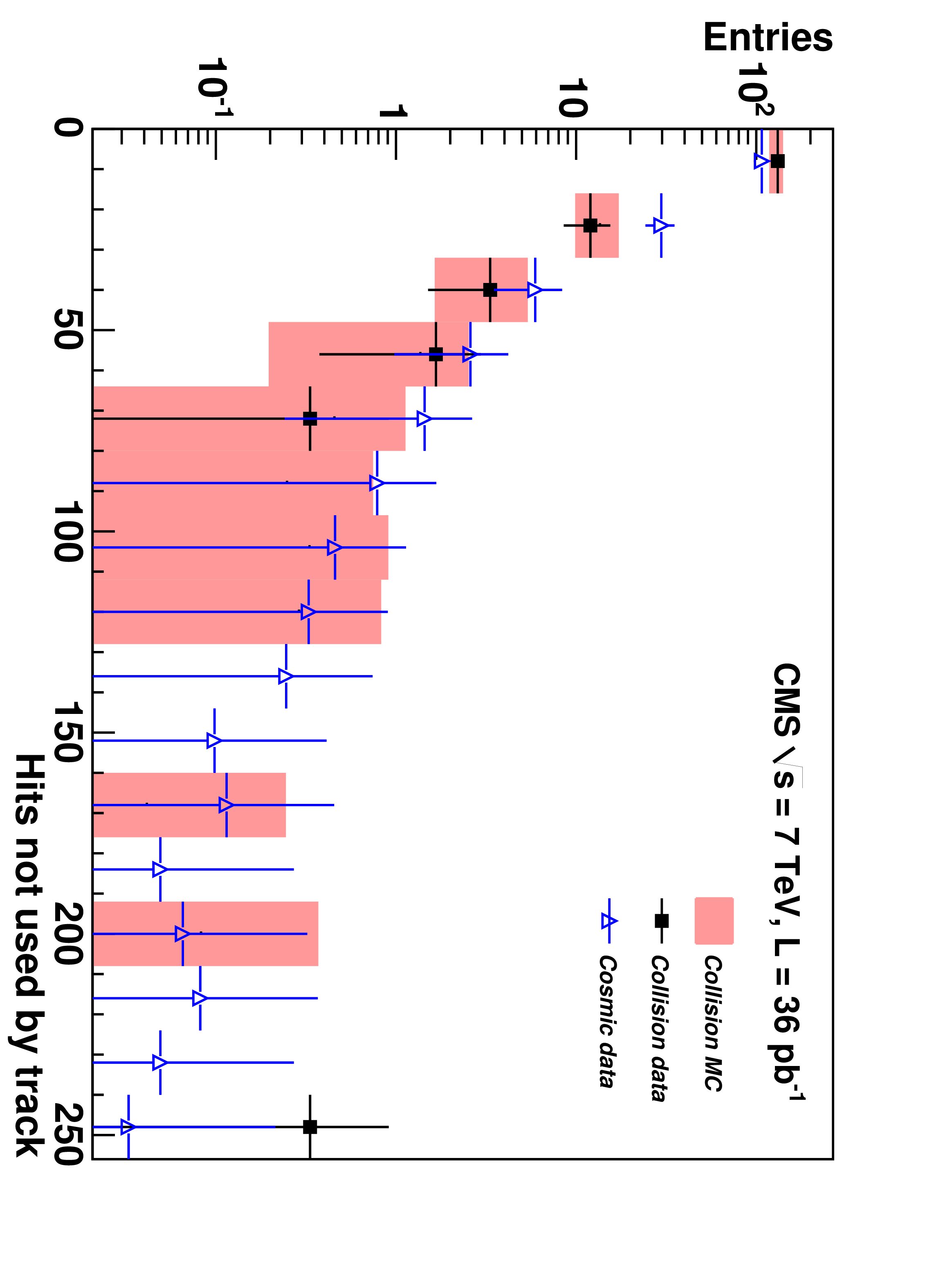
Figure 10-a:
Comparison of data and simulation for variables characterizing electromagnetic showers, for muons with $p >$ 150 GeV/$c$ in the barrel region: the number of reconstructed muon hits not used in a track fit (left); the transverse size of the cluster of hits around a track (right). All distributions are normalized to the number of muons per muon station in the collision data sample. |
png pdf |
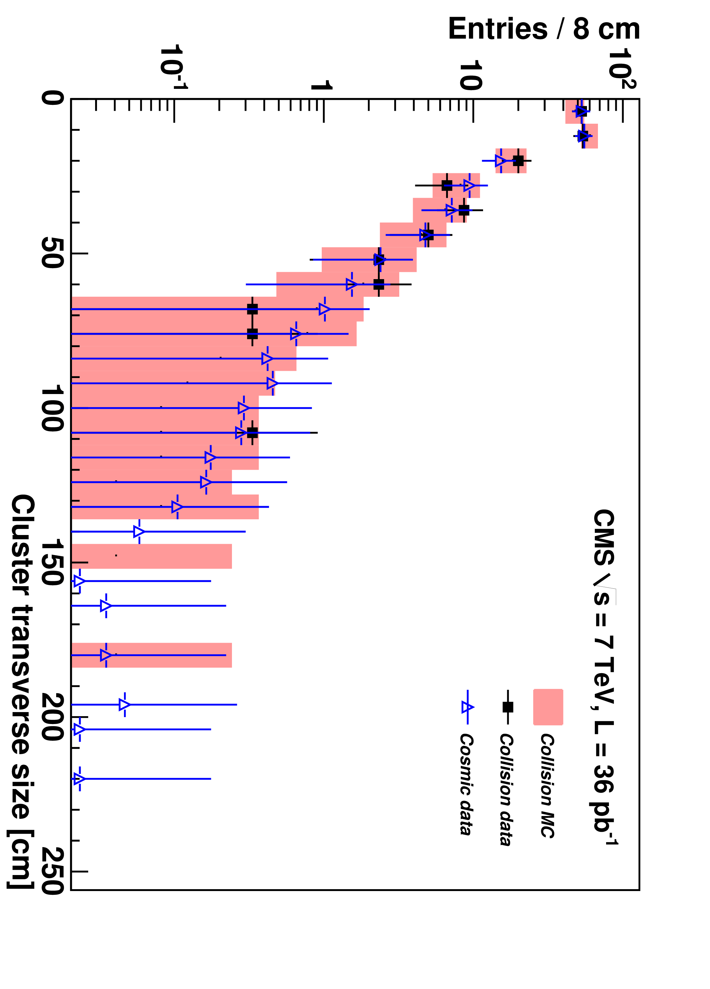
Figure 10-b:
Comparison of data and simulation for variables characterizing electromagnetic showers, for muons with $p >$ 150 GeV/$c$ in the barrel region: the number of reconstructed muon hits not used in a track fit (left); the transverse size of the cluster of hits around a track (right). All distributions are normalized to the number of muons per muon station in the collision data sample. |
png pdf |
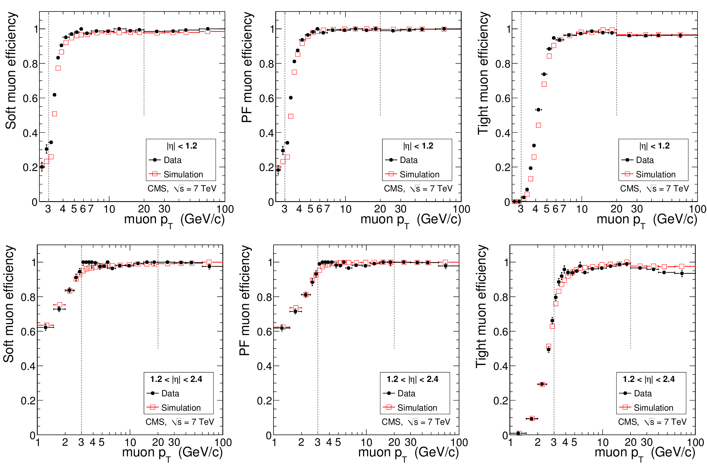
Figure 11:
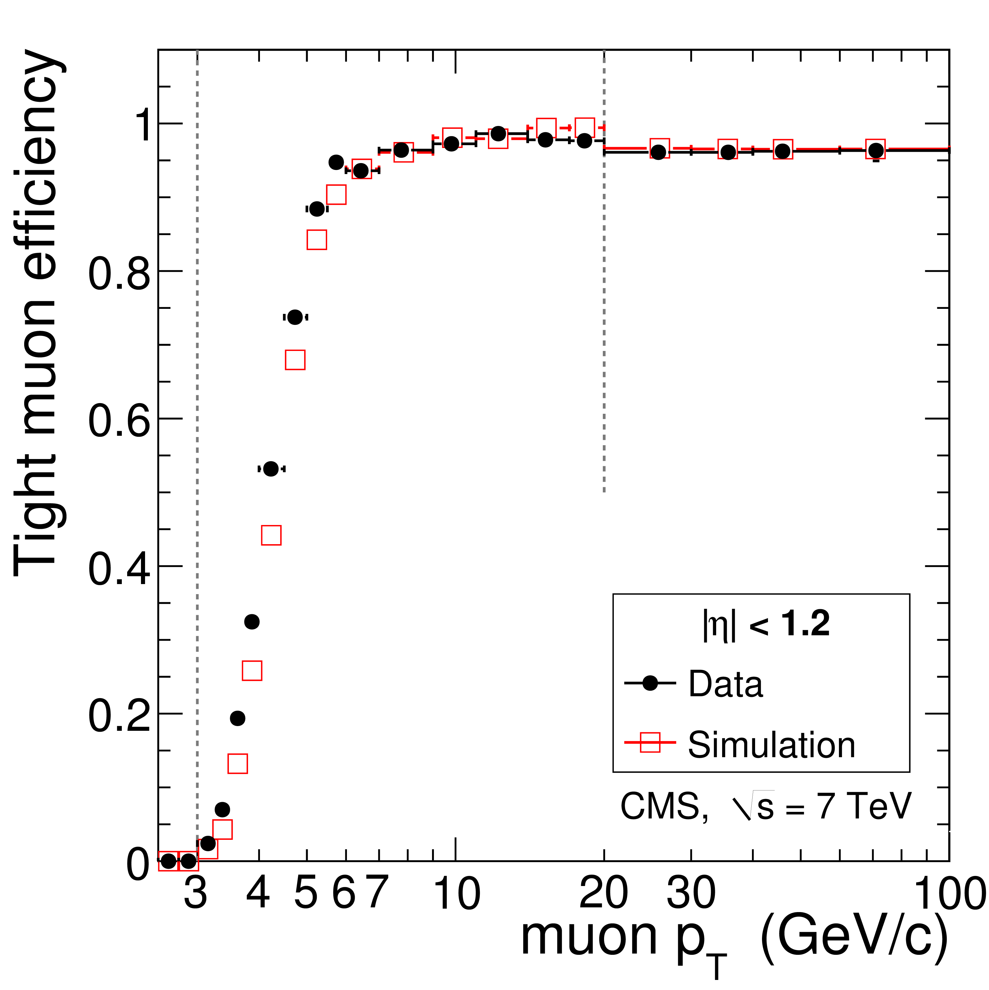
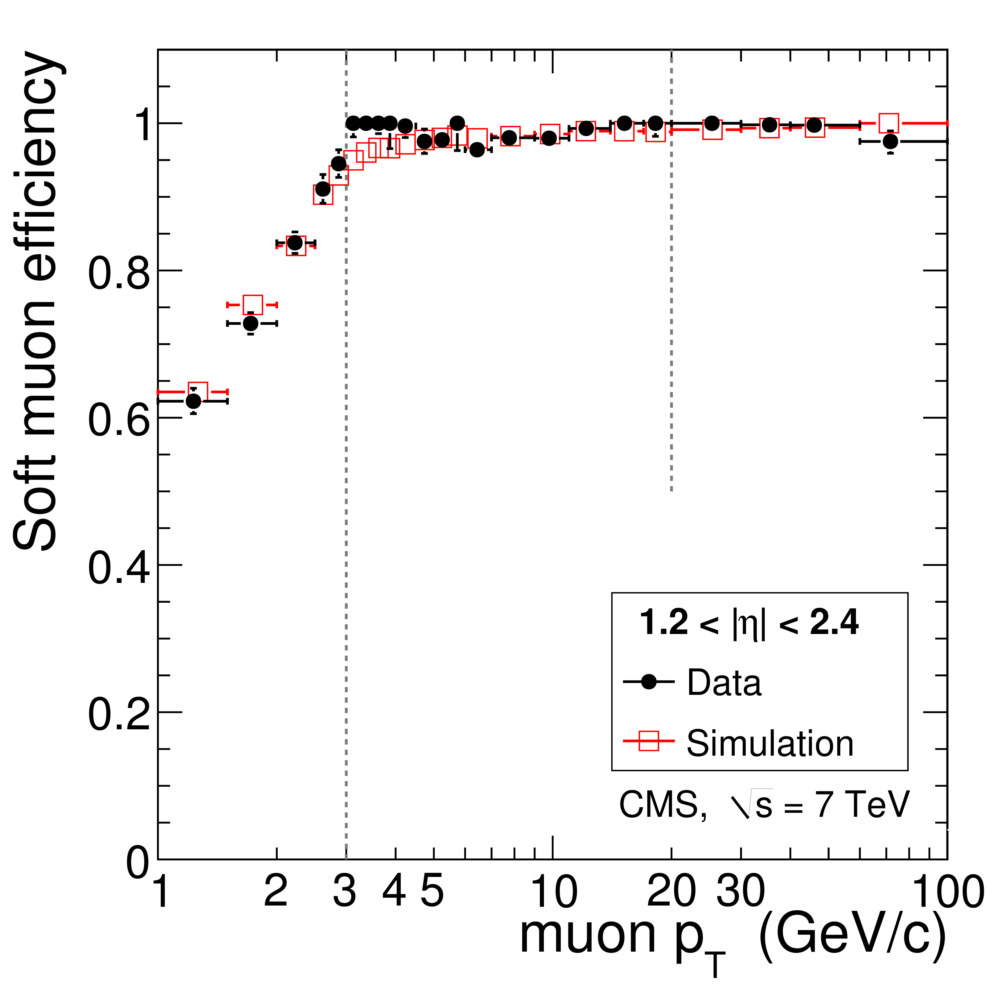
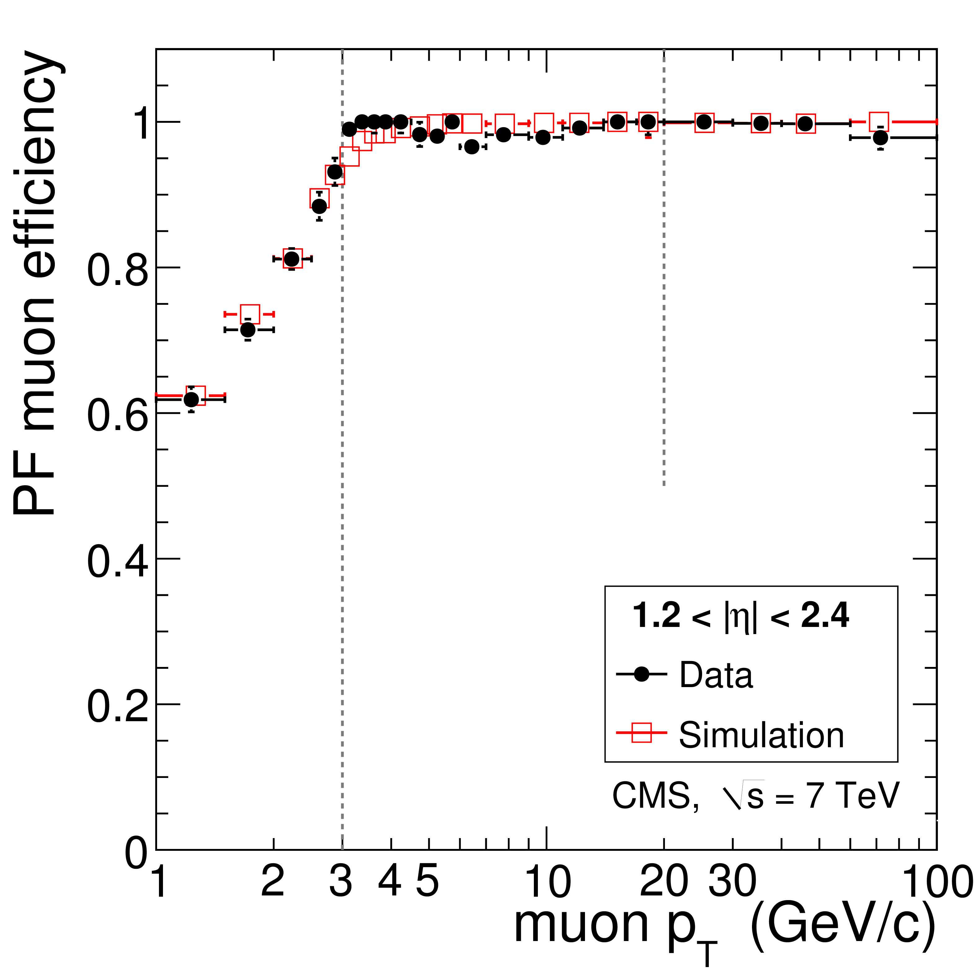
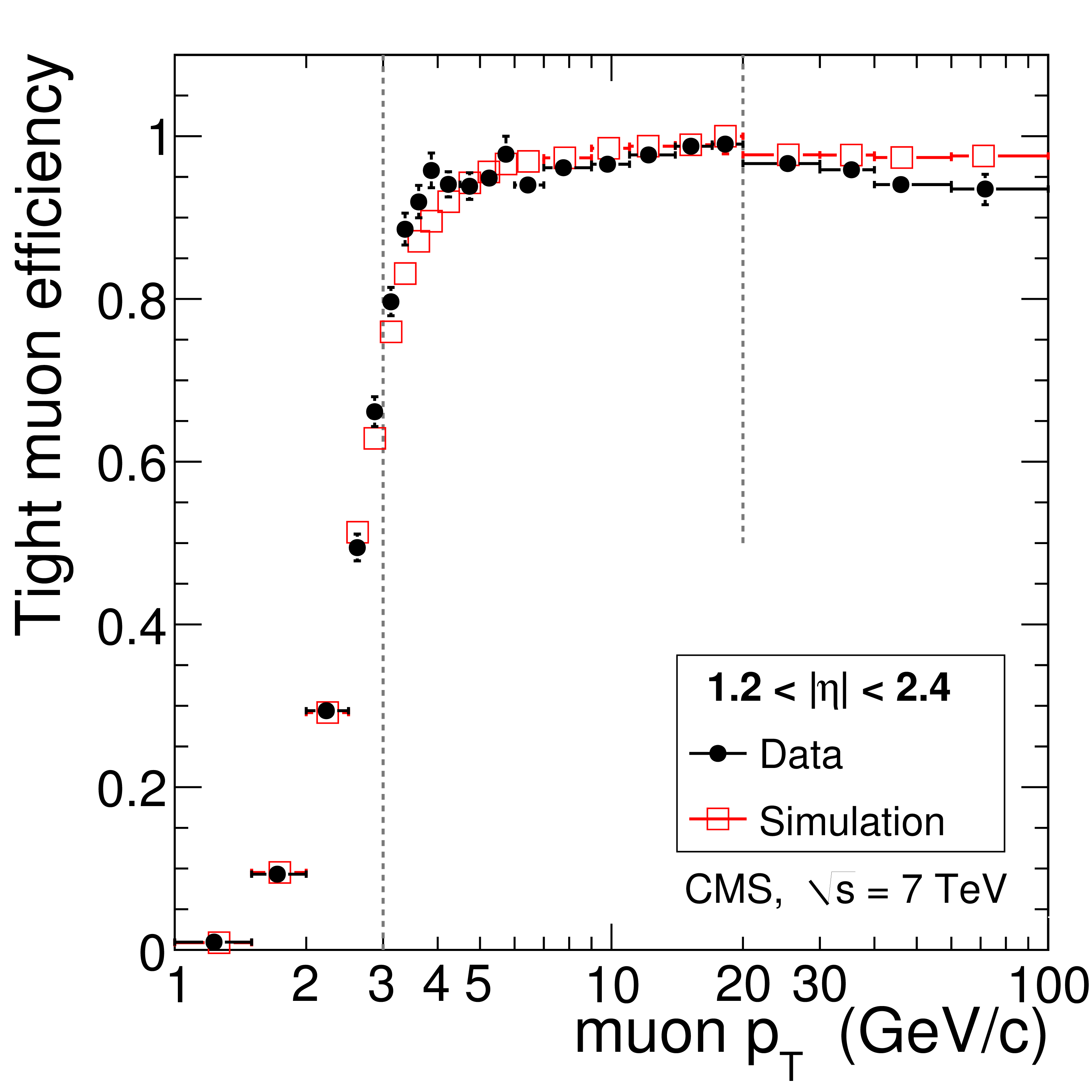
Tag-and-probe results for the muon efficiency $\epsilon _{\mathrm {rec+id}}$ in data compared to simulation. Given that a tracker track exists, the plots show the efficiency as a function of muon $ {p_{\mathrm {T}}} $ for Soft Muons (left), Particle-Flow Muons (middle), and Tight Muons (right) in the barrel and overlap regions (top), and in the endcaps (bottom). The measurement is made using $\mathrm {J}/\psi \to \mu ^+\mu ^-$ events for $ {p_{\mathrm {T}}} < $ 20 GeV/$c$ and $ {\mathrm {Z}}\to \mu ^+\mu ^-$ events for $ {p_{\mathrm {T}}} > $ 20 GeV/$c$. For $ {p_{\mathrm {T}}} < $ 3 GeV/$c$, to reduce the background, only tracks with MIP signature are considered. |

png pdf |
Figure 11-a:
Tag-and-probe results for the muon efficiency $\epsilon _{\mathrm {rec+id}}$ in data compared to simulation. Given that a tracker track exists, the plots show the efficiency as a function of muon $ {p_{\mathrm {T}}} $ for Soft Muons (left), Particle-Flow Muons (middle), and Tight Muons (right) in the barrel and overlap regions (top), and in the endcaps (bottom). The measurement is made using $\mathrm {J}/\psi \to \mu ^+\mu ^-$ events for $ {p_{\mathrm {T}}} < $ 20 GeV/$c$ and $ {\mathrm {Z}}\to \mu ^+\mu ^-$ events for $ {p_{\mathrm {T}}} > $ 20 GeV/$c$. For $ {p_{\mathrm {T}}} < $ 3 GeV/$c$, to reduce the background, only tracks with MIP signature are considered. |

png pdf |
Figure 11-b:
Tag-and-probe results for the muon efficiency $\epsilon _{\mathrm {rec+id}}$ in data compared to simulation. Given that a tracker track exists, the plots show the efficiency as a function of muon $ {p_{\mathrm {T}}} $ for Soft Muons (left), Particle-Flow Muons (middle), and Tight Muons (right) in the barrel and overlap regions (top), and in the endcaps (bottom). The measurement is made using $\mathrm {J}/\psi \to \mu ^+\mu ^-$ events for $ {p_{\mathrm {T}}} < $ 20 GeV/$c$ and $ {\mathrm {Z}}\to \mu ^+\mu ^-$ events for $ {p_{\mathrm {T}}} > $ 20 GeV/$c$. For $ {p_{\mathrm {T}}} < $ 3 GeV/$c$, to reduce the background, only tracks with MIP signature are considered. |
png pdf |
Figure 11-c:
Tag-and-probe results for the muon efficiency $\epsilon _{\mathrm {rec+id}}$ in data compared to simulation. Given that a tracker track exists, the plots show the efficiency as a function of muon $ {p_{\mathrm {T}}} $ for Soft Muons (left), Particle-Flow Muons (middle), and Tight Muons (right) in the barrel and overlap regions (top), and in the endcaps (bottom). The measurement is made using $\mathrm {J}/\psi \to \mu ^+\mu ^-$ events for $ {p_{\mathrm {T}}} < $ 20 GeV/$c$ and $ {\mathrm {Z}}\to \mu ^+\mu ^-$ events for $ {p_{\mathrm {T}}} > $ 20 GeV/$c$. For $ {p_{\mathrm {T}}} < $ 3 GeV/$c$, to reduce the background, only tracks with MIP signature are considered. |
png pdf |
Figure 11-d:
Tag-and-probe results for the muon efficiency $\epsilon _{\mathrm {rec+id}}$ in data compared to simulation. Given that a tracker track exists, the plots show the efficiency as a function of muon $ {p_{\mathrm {T}}} $ for Soft Muons (left), Particle-Flow Muons (middle), and Tight Muons (right) in the barrel and overlap regions (top), and in the endcaps (bottom). The measurement is made using $\mathrm {J}/\psi \to \mu ^+\mu ^-$ events for $ {p_{\mathrm {T}}} < $ 20 GeV/$c$ and $ {\mathrm {Z}}\to \mu ^+\mu ^-$ events for $ {p_{\mathrm {T}}} > $ 20 GeV/$c$. For $ {p_{\mathrm {T}}} < $ 3 GeV/$c$, to reduce the background, only tracks with MIP signature are considered. |
png pdf |
Figure 11-e:
Tag-and-probe results for the muon efficiency $\epsilon _{\mathrm {rec+id}}$ in data compared to simulation. Given that a tracker track exists, the plots show the efficiency as a function of muon $ {p_{\mathrm {T}}} $ for Soft Muons (left), Particle-Flow Muons (middle), and Tight Muons (right) in the barrel and overlap regions (top), and in the endcaps (bottom). The measurement is made using $\mathrm {J}/\psi \to \mu ^+\mu ^-$ events for $ {p_{\mathrm {T}}} < $ 20 GeV/$c$ and $ {\mathrm {Z}}\to \mu ^+\mu ^-$ events for $ {p_{\mathrm {T}}} > $ 20 GeV/$c$. For $ {p_{\mathrm {T}}} < $ 3 GeV/$c$, to reduce the background, only tracks with MIP signature are considered. |
png pdf |
Figure 11-f:
Tag-and-probe results for the muon efficiency $\epsilon _{\mathrm {rec+id}}$ in data compared to simulation. Given that a tracker track exists, the plots show the efficiency as a function of muon $ {p_{\mathrm {T}}} $ for Soft Muons (left), Particle-Flow Muons (middle), and Tight Muons (right) in the barrel and overlap regions (top), and in the endcaps (bottom). The measurement is made using $\mathrm {J}/\psi \to \mu ^+\mu ^-$ events for $ {p_{\mathrm {T}}} < $ 20 GeV/$c$ and $ {\mathrm {Z}}\to \mu ^+\mu ^-$ events for $ {p_{\mathrm {T}}} > $ 20 GeV/$c$. For $ {p_{\mathrm {T}}} < $ 3 GeV/$c$, to reduce the background, only tracks with MIP signature are considered. |

png pdf |
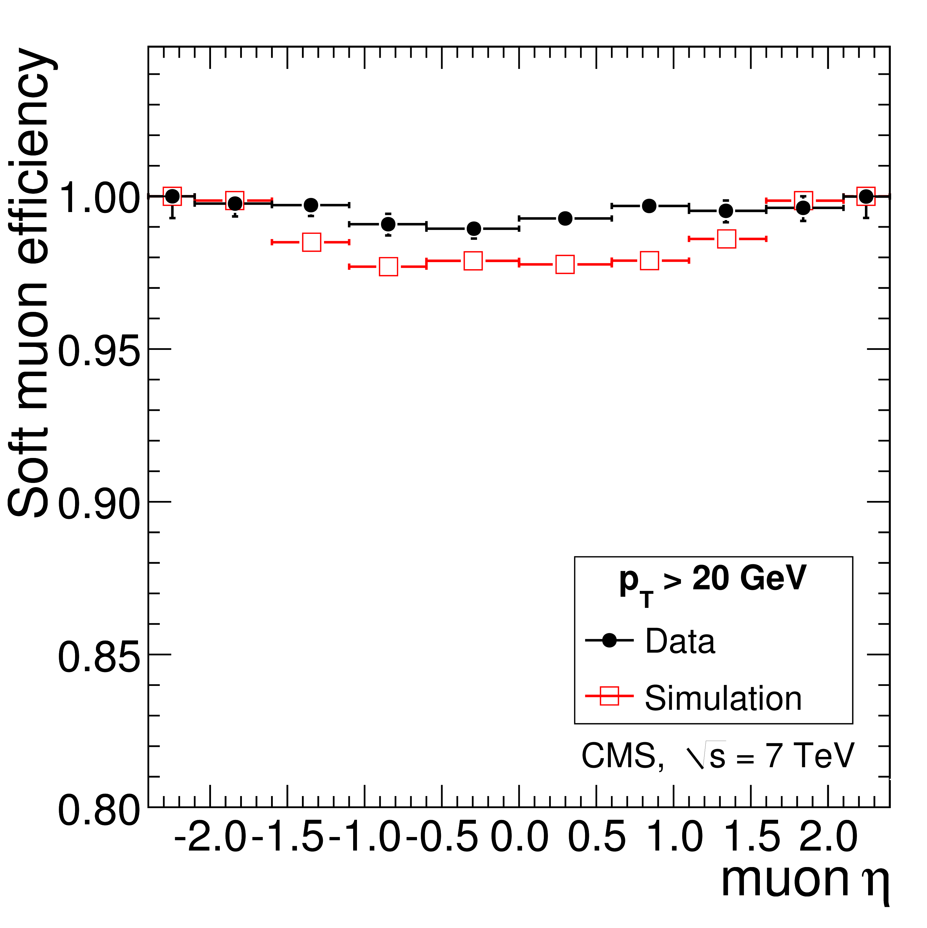
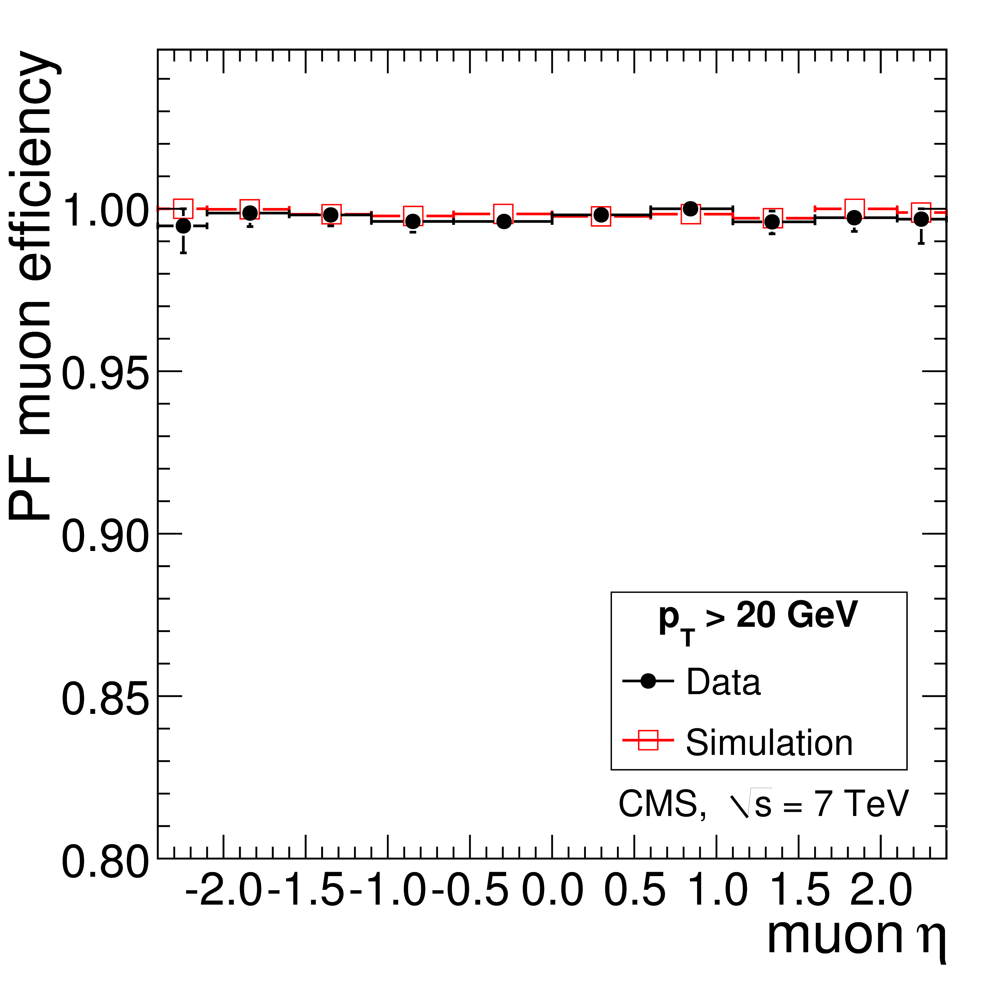
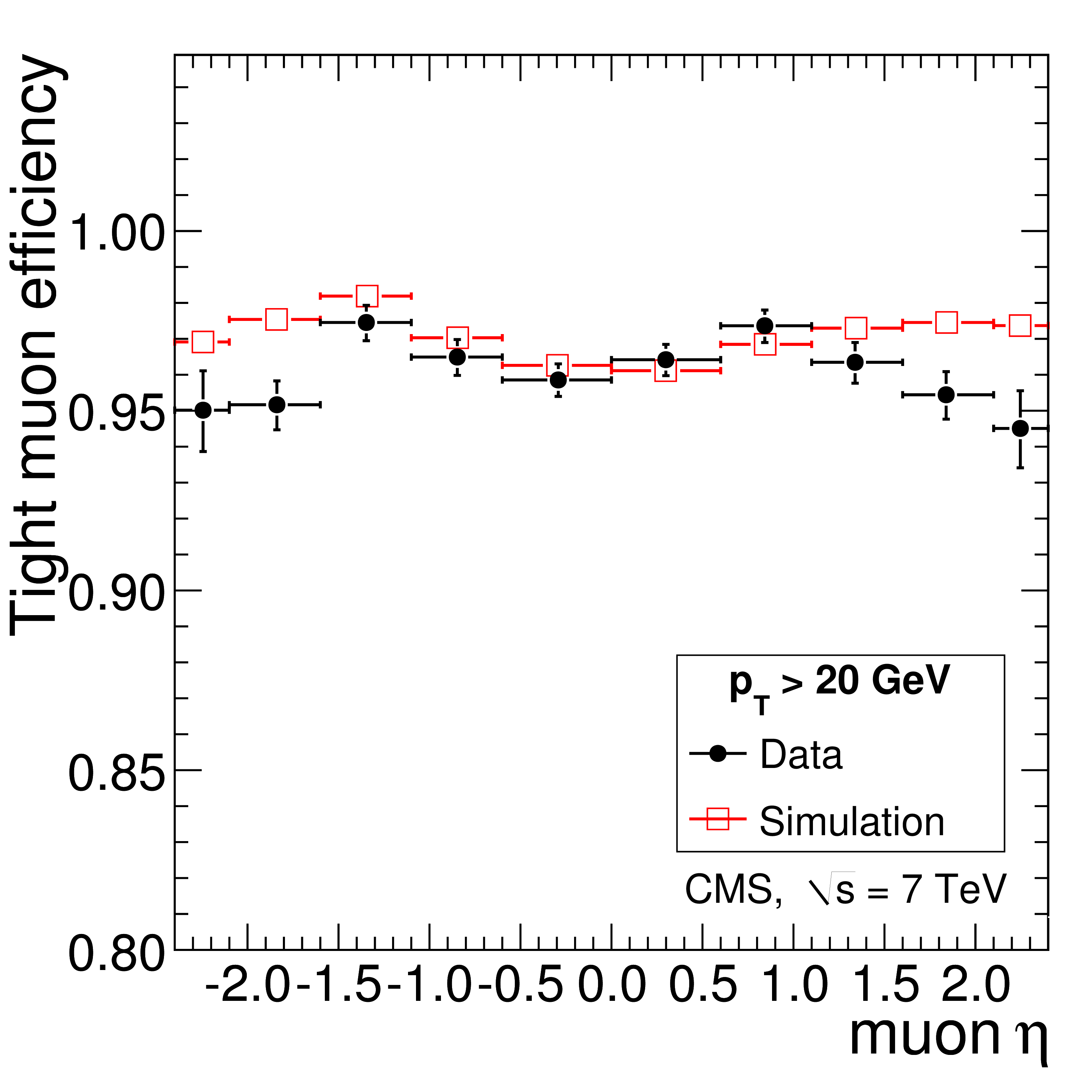
Figure 12:
Muon efficiency $\epsilon _{\mathrm {rec+id}}$ in data and simulation as a function of muon pseudorapidity for Soft Muons (left), Particle-Flow Muons (middle), and Tight Muons (right). The efficiencies were calculated relative to the tracker tracks with $ {p_{\mathrm {T}}} > $ 20 GeV/$c$ by applying the tag-and-probe technique to $ {\mathrm {Z}}\to \mu ^+\mu ^-$ events. |
png pdf |
Figure 12-a:
Muon efficiency $\epsilon _{\mathrm {rec+id}}$ in data and simulation as a function of muon pseudorapidity for Soft Muons (left), Particle-Flow Muons (middle), and Tight Muons (right). The efficiencies were calculated relative to the tracker tracks with $ {p_{\mathrm {T}}} > $ 20 GeV/$c$ by applying the tag-and-probe technique to $ {\mathrm {Z}}\to \mu ^+\mu ^-$ events. |
png pdf |
Figure 12-b:
Muon efficiency $\epsilon _{\mathrm {rec+id}}$ in data and simulation as a function of muon pseudorapidity for Soft Muons (left), Particle-Flow Muons (middle), and Tight Muons (right). The efficiencies were calculated relative to the tracker tracks with $ {p_{\mathrm {T}}} > $ 20 GeV/$c$ by applying the tag-and-probe technique to $ {\mathrm {Z}}\to \mu ^+\mu ^-$ events. |
png pdf |
Figure 12-c:
Muon efficiency $\epsilon _{\mathrm {rec+id}}$ in data and simulation as a function of muon pseudorapidity for Soft Muons (left), Particle-Flow Muons (middle), and Tight Muons (right). The efficiencies were calculated relative to the tracker tracks with $ {p_{\mathrm {T}}} > $ 20 GeV/$c$ by applying the tag-and-probe technique to $ {\mathrm {Z}}\to \mu ^+\mu ^-$ events. |
png pdf |
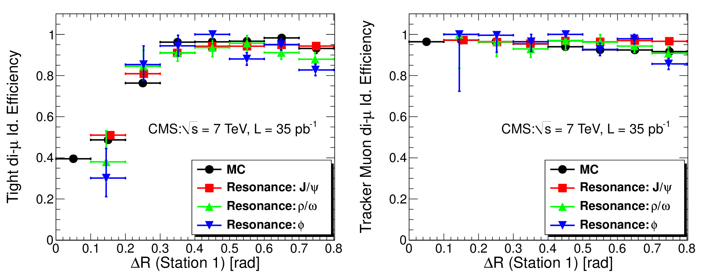
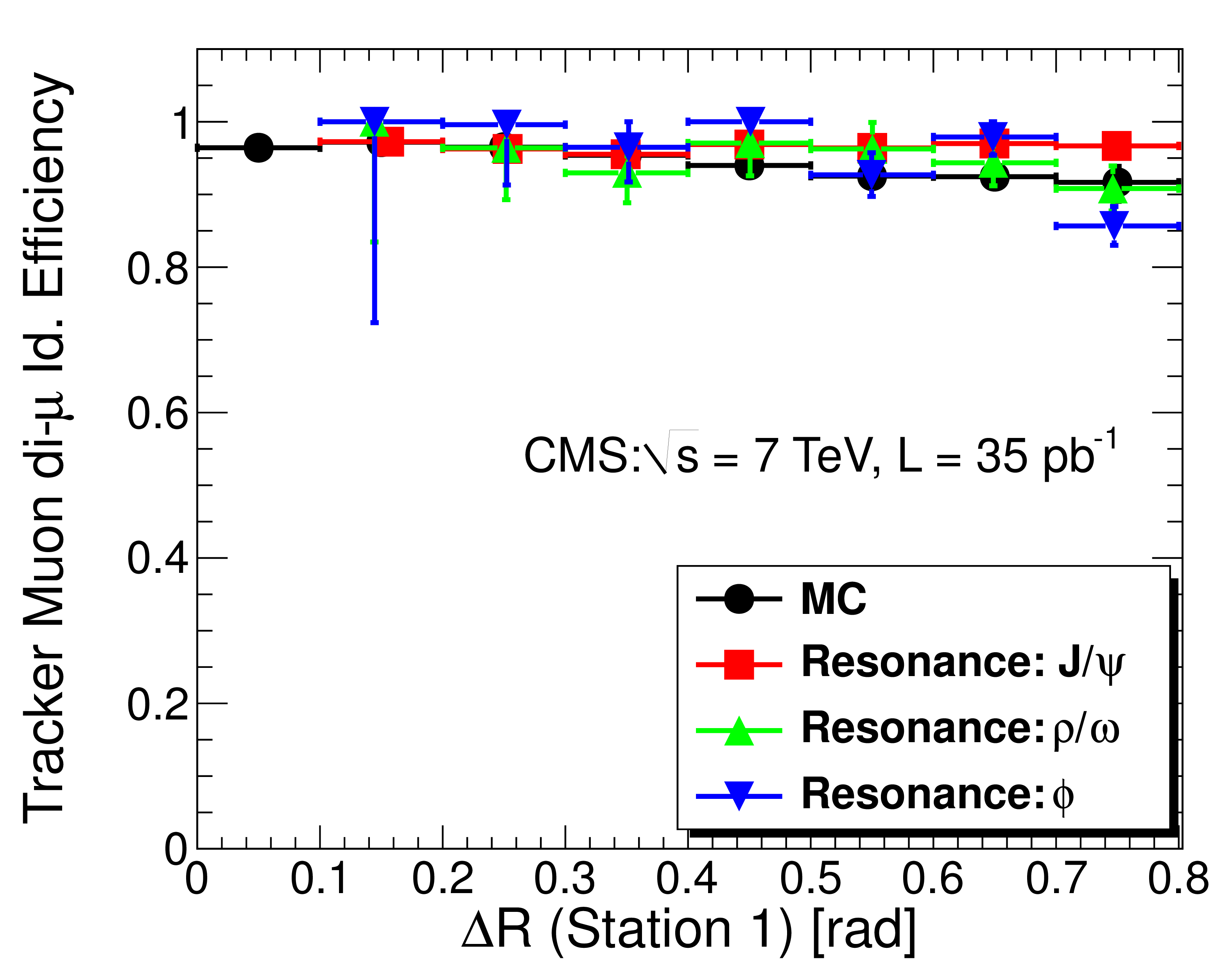
Figure 13:
Efficiency for identifying both muons in the dimuon pair as Tight (left) and Tracker (right) Muons as a function of the angular separation of the two tracks computed at the surface of the first muon station. Measurements obtained using $\mathrm {J}/\psi $ (squares), $\phi $ (inverted triangles), and $\rho $/$\omega $ (triangles) are compared with the expectations from the simulation (circles). |

png pdf |
Figure 13-a:
Efficiency for identifying both muons in the dimuon pair as Tight (left) and Tracker (right) Muons as a function of the angular separation of the two tracks computed at the surface of the first muon station. Measurements obtained using $\mathrm {J}/\psi $ (squares), $\phi $ (inverted triangles), and $\rho $/$\omega $ (triangles) are compared with the expectations from the simulation (circles). |
png pdf |
Figure 13-b:
Efficiency for identifying both muons in the dimuon pair as Tight (left) and Tracker (right) Muons as a function of the angular separation of the two tracks computed at the surface of the first muon station. Measurements obtained using $\mathrm {J}/\psi $ (squares), $\phi $ (inverted triangles), and $\rho $/$\omega $ (triangles) are compared with the expectations from the simulation (circles). |
png pdf |
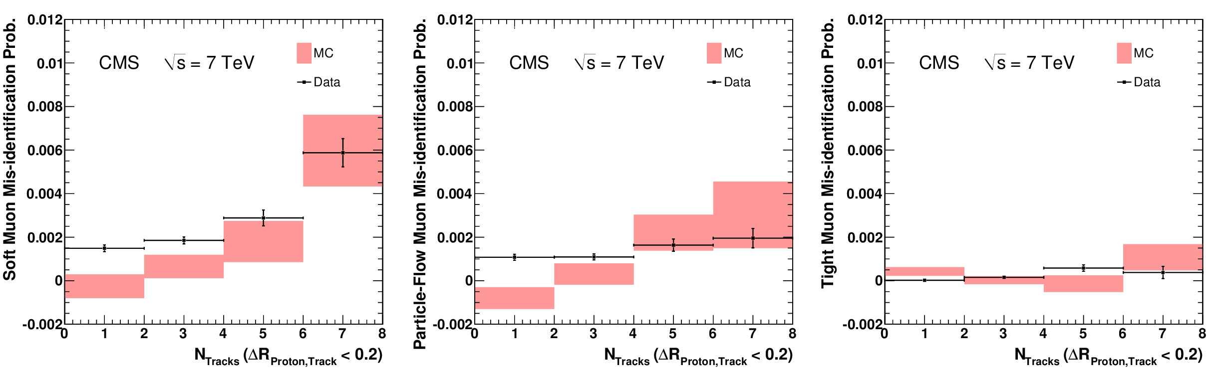
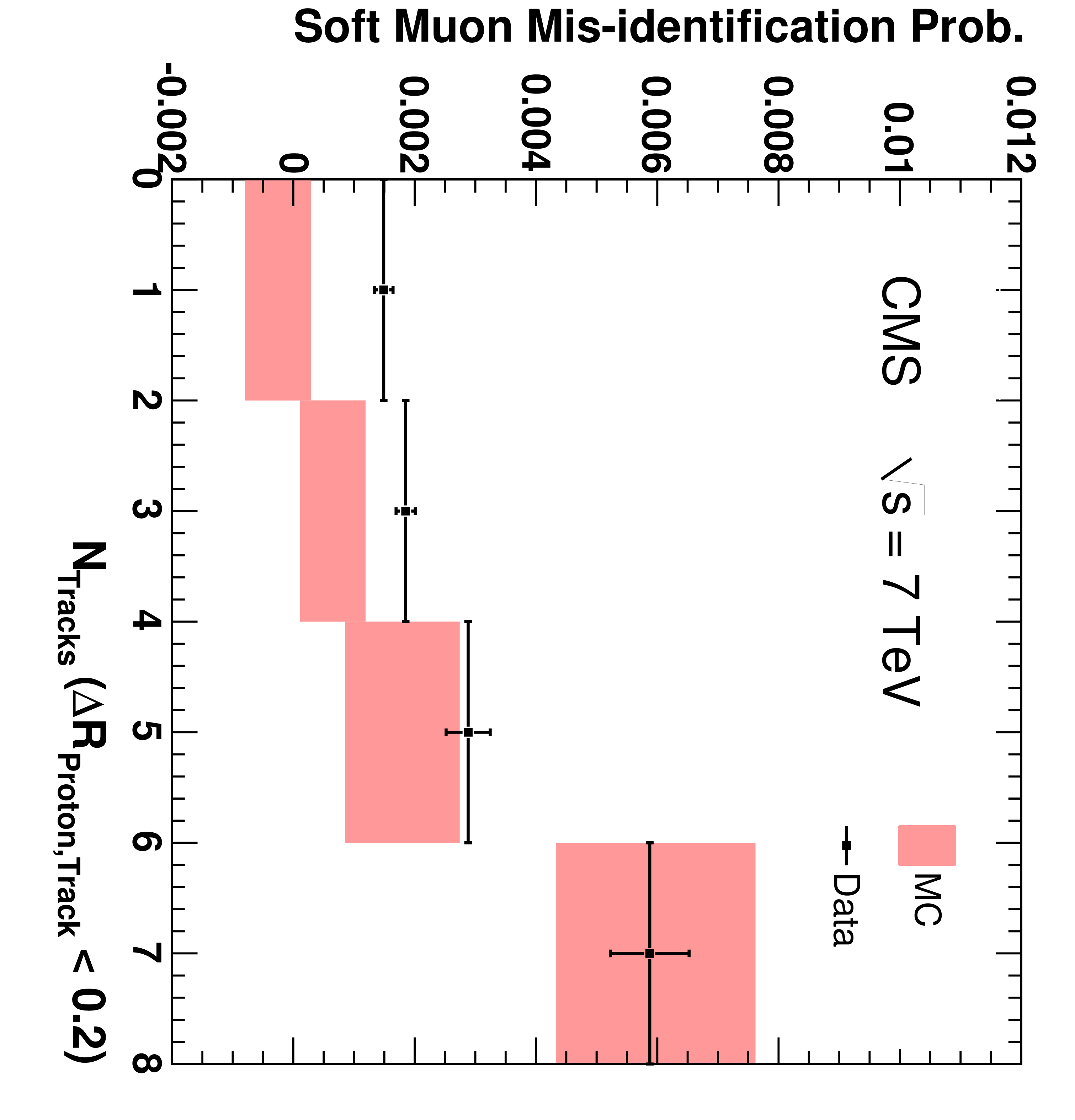
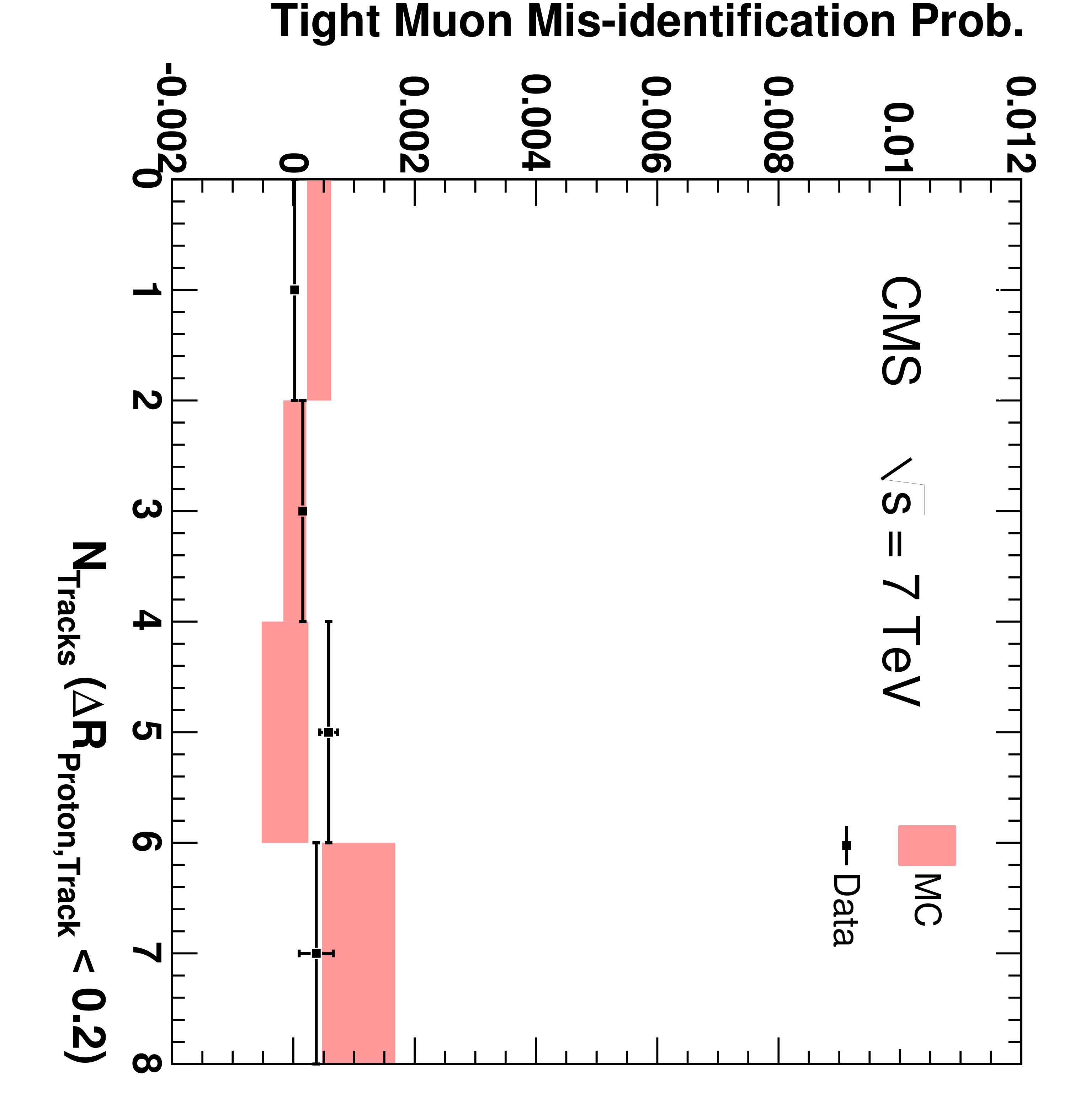
Figure 14:
The fraction of protons that are misidentified as a Soft Muon (left), Particle-Flow Muon (centre), or Tight Muon (right) as a function of $N_{\mathrm {Tracks}}$, where $N_{\mathrm {Tracks}}$ represents the number of tracks in the vicinity of the proton track (with ${\Delta }R = \sqrt {(\Delta \eta )^2 + (\Delta \phi )^2} < 0.2$). Only protons with $p > $ 3 GeV/$c$ are included. The first bin includes events with $N_{\mathrm {Tracks}} = 0$ and 1, the second bin includes those with $N_{\mathrm {Tracks}} = 2$ and 3, etc. The uncertainties indicated by the error bars (data) and shaded boxes (PYTHIA simulation) are statistical only. Negative values arise from statistical fluctuations in the number of events in the signal and sideband regions. |
png pdf |
Figure 14-a:
The fraction of protons that are misidentified as a Soft Muon (left), Particle-Flow Muon (centre), or Tight Muon (right) as a function of $N_{\mathrm {Tracks}}$, where $N_{\mathrm {Tracks}}$ represents the number of tracks in the vicinity of the proton track (with ${\Delta }R = \sqrt {(\Delta \eta )^2 + (\Delta \phi )^2} < 0.2$). Only protons with $p > $ 3 GeV/$c$ are included. The first bin includes events with $N_{\mathrm {Tracks}} = 0$ and 1, the second bin includes those with $N_{\mathrm {Tracks}} = 2$ and 3, etc. The uncertainties indicated by the error bars (data) and shaded boxes (PYTHIA simulation) are statistical only. Negative values arise from statistical fluctuations in the number of events in the signal and sideband regions. |

png pdf |
Figure 14-b:
The fraction of protons that are misidentified as a Soft Muon (left), Particle-Flow Muon (centre), or Tight Muon (right) as a function of $N_{\mathrm {Tracks}}$, where $N_{\mathrm {Tracks}}$ represents the number of tracks in the vicinity of the proton track (with ${\Delta }R = \sqrt {(\Delta \eta )^2 + (\Delta \phi )^2} < 0.2$). Only protons with $p > $ 3 GeV/$c$ are included. The first bin includes events with $N_{\mathrm {Tracks}} = 0$ and 1, the second bin includes those with $N_{\mathrm {Tracks}} = 2$ and 3, etc. The uncertainties indicated by the error bars (data) and shaded boxes (PYTHIA simulation) are statistical only. Negative values arise from statistical fluctuations in the number of events in the signal and sideband regions. |
png pdf |
Figure 14-c:
The fraction of protons that are misidentified as a Soft Muon (left), Particle-Flow Muon (centre), or Tight Muon (right) as a function of $N_{\mathrm {Tracks}}$, where $N_{\mathrm {Tracks}}$ represents the number of tracks in the vicinity of the proton track (with ${\Delta }R = \sqrt {(\Delta \eta )^2 + (\Delta \phi )^2} < 0.2$). Only protons with $p > $ 3 GeV/$c$ are included. The first bin includes events with $N_{\mathrm {Tracks}} = 0$ and 1, the second bin includes those with $N_{\mathrm {Tracks}} = 2$ and 3, etc. The uncertainties indicated by the error bars (data) and shaded boxes (PYTHIA simulation) are statistical only. Negative values arise from statistical fluctuations in the number of events in the signal and sideband regions. |

png pdf |
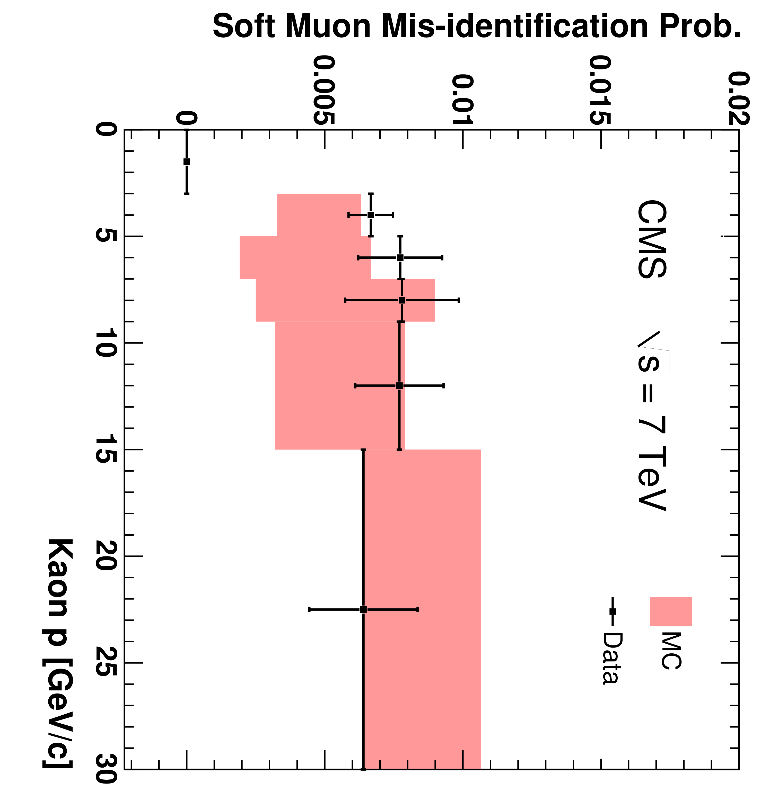
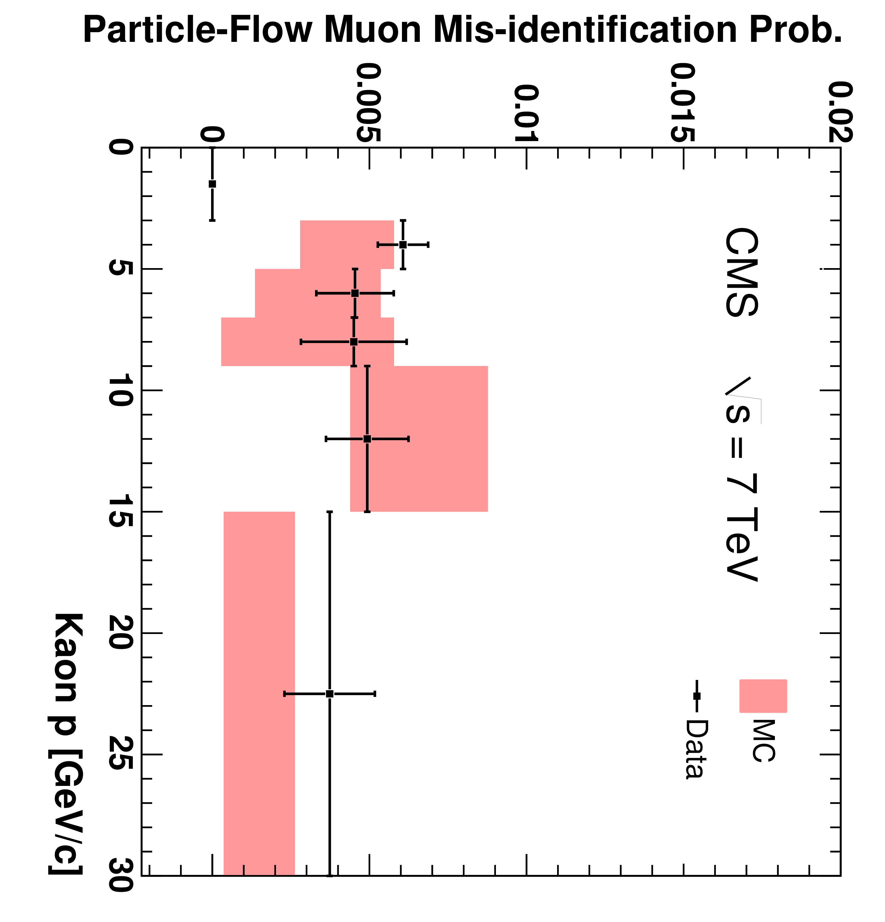
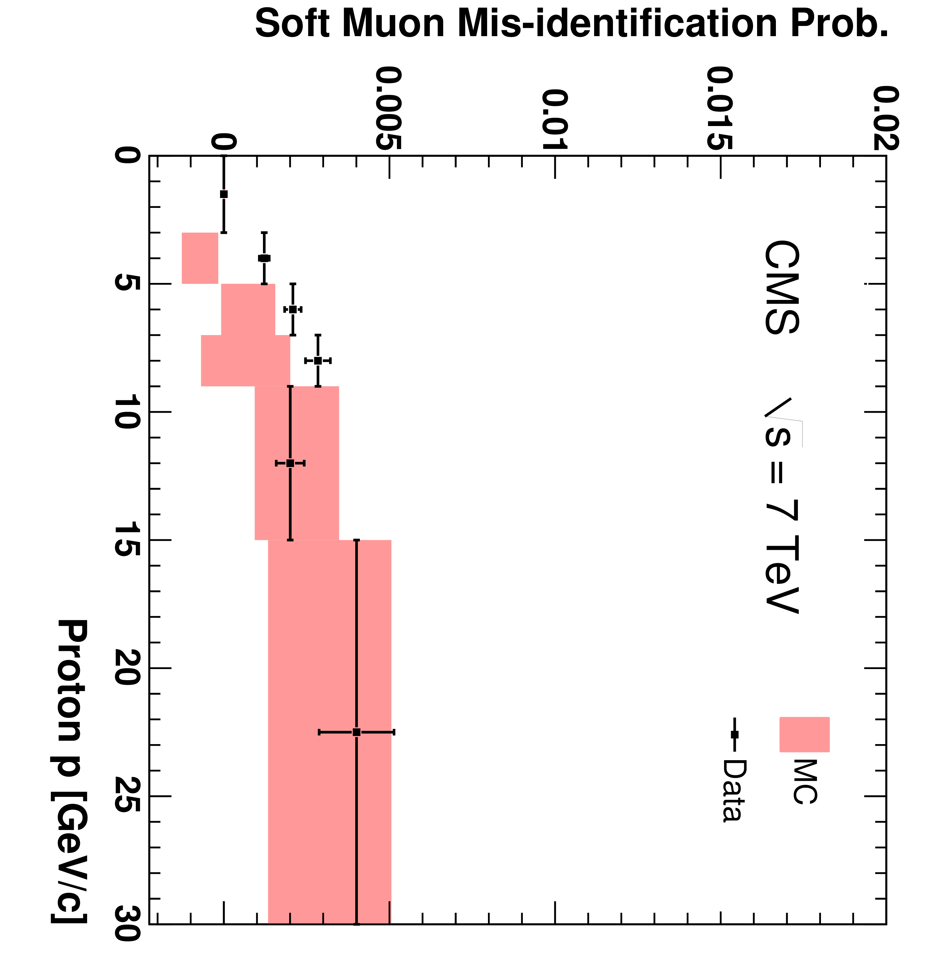
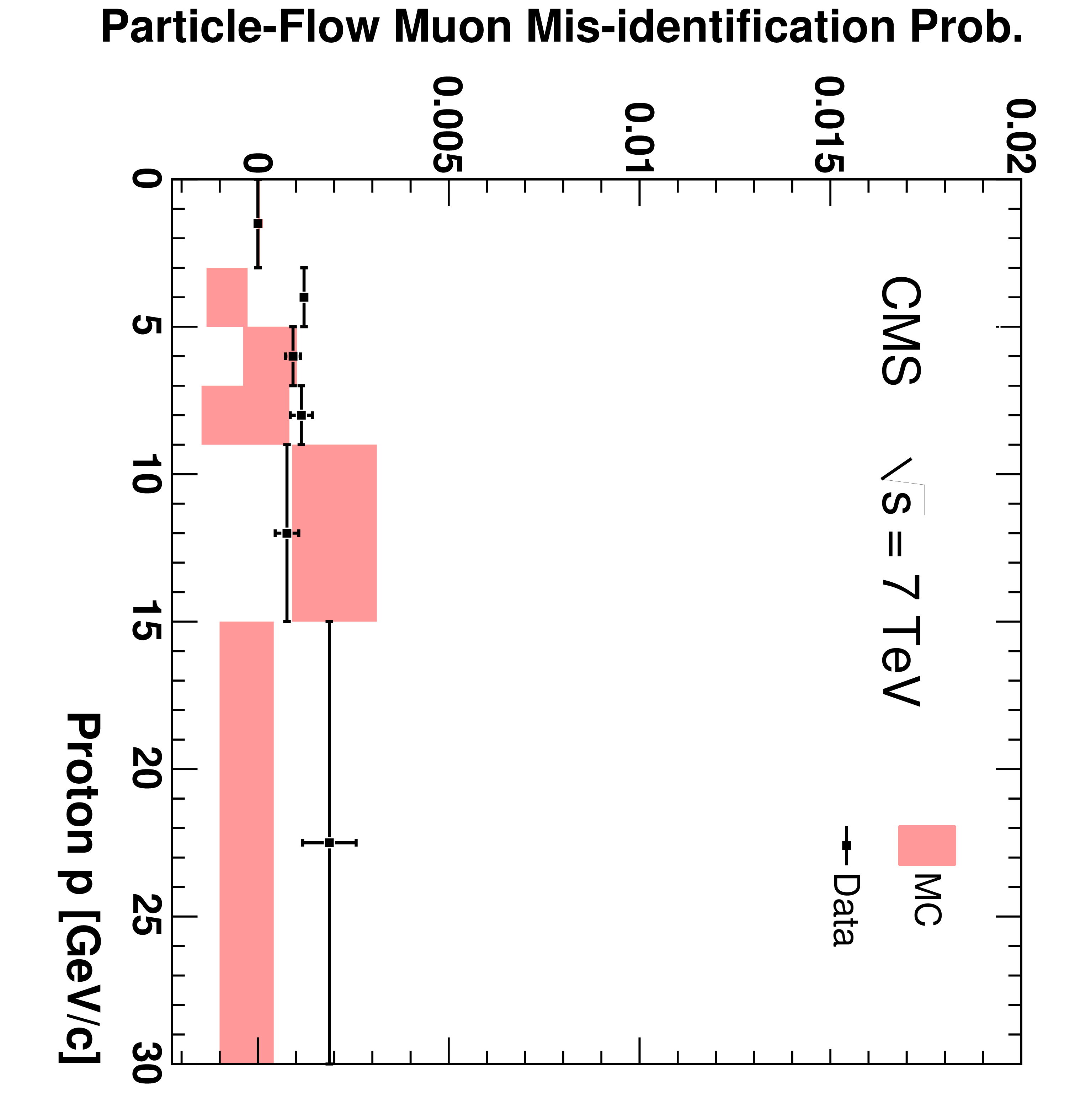
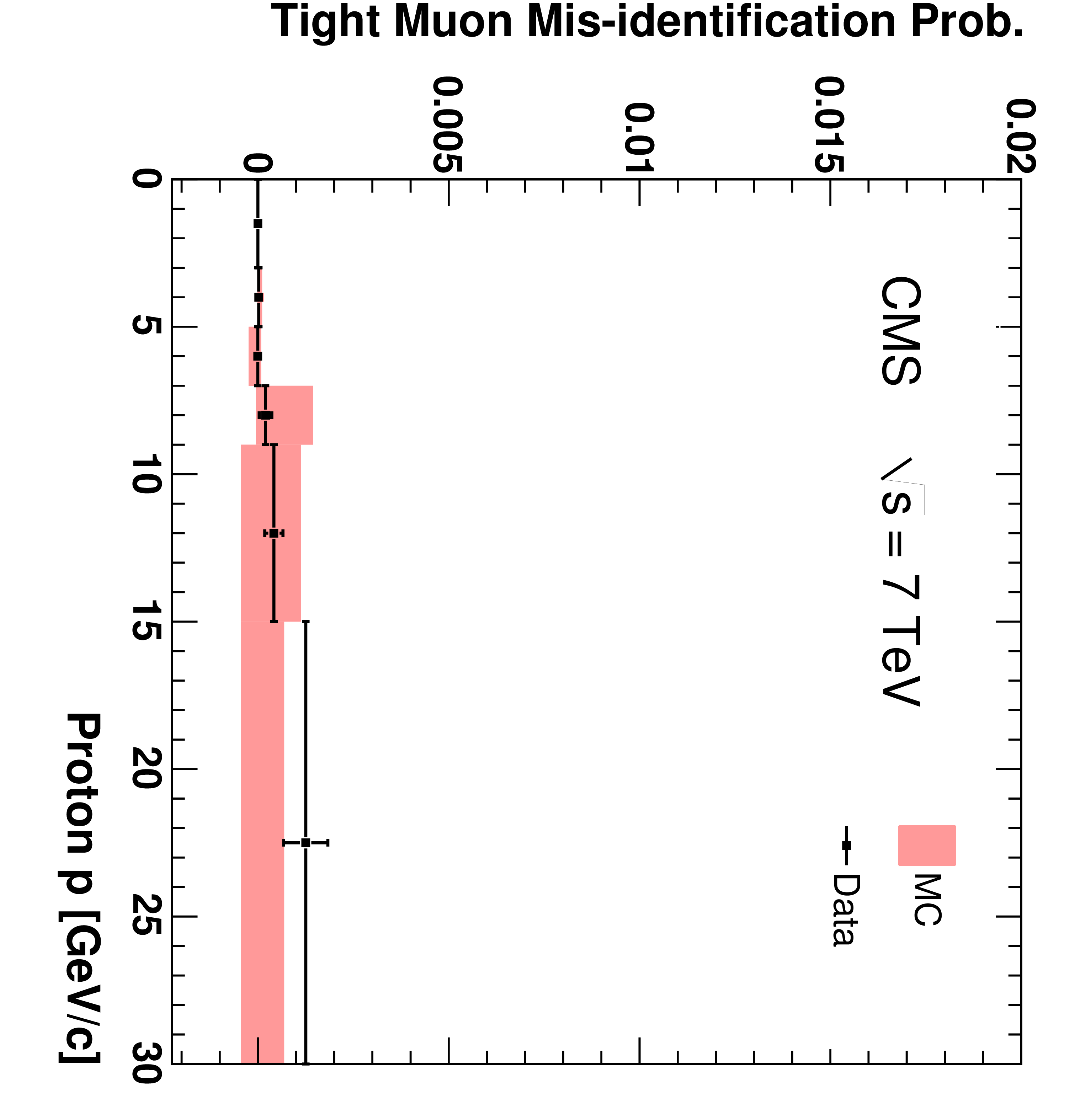
Figure 15:
The fractions of pions (top), kaons (centre), and protons (bottom) that are misidentified as Soft Muons (left), Particle-Flow Muons (centre), or Tight Muons (right) as a function of momentum. Only particles with $N_{\mathrm {Tracks}} < 4$ are included. The uncertainties indicated by the error bars (data) and shaded boxes (PYTHIA simulation) are statistical only. |

png pdf |
Figure 15-a:
The fractions of pions (top), kaons (centre), and protons (bottom) that are misidentified as Soft Muons (left), Particle-Flow Muons (centre), or Tight Muons (right) as a function of momentum. Only particles with $N_{\mathrm {Tracks}} < 4$ are included. The uncertainties indicated by the error bars (data) and shaded boxes (PYTHIA simulation) are statistical only. |

png pdf |
Figure 15-b:
The fractions of pions (top), kaons (centre), and protons (bottom) that are misidentified as Soft Muons (left), Particle-Flow Muons (centre), or Tight Muons (right) as a function of momentum. Only particles with $N_{\mathrm {Tracks}} < 4$ are included. The uncertainties indicated by the error bars (data) and shaded boxes (PYTHIA simulation) are statistical only. |

png pdf |
Figure 15-c:
The fractions of pions (top), kaons (centre), and protons (bottom) that are misidentified as Soft Muons (left), Particle-Flow Muons (centre), or Tight Muons (right) as a function of momentum. Only particles with $N_{\mathrm {Tracks}} < 4$ are included. The uncertainties indicated by the error bars (data) and shaded boxes (PYTHIA simulation) are statistical only. |
png pdf |
Figure 15-d:
The fractions of pions (top), kaons (centre), and protons (bottom) that are misidentified as Soft Muons (left), Particle-Flow Muons (centre), or Tight Muons (right) as a function of momentum. Only particles with $N_{\mathrm {Tracks}} < 4$ are included. The uncertainties indicated by the error bars (data) and shaded boxes (PYTHIA simulation) are statistical only. |
png pdf |
Figure 15-e:
The fractions of pions (top), kaons (centre), and protons (bottom) that are misidentified as Soft Muons (left), Particle-Flow Muons (centre), or Tight Muons (right) as a function of momentum. Only particles with $N_{\mathrm {Tracks}} < 4$ are included. The uncertainties indicated by the error bars (data) and shaded boxes (PYTHIA simulation) are statistical only. |

png pdf |
Figure 15-f:
The fractions of pions (top), kaons (centre), and protons (bottom) that are misidentified as Soft Muons (left), Particle-Flow Muons (centre), or Tight Muons (right) as a function of momentum. Only particles with $N_{\mathrm {Tracks}} < 4$ are included. The uncertainties indicated by the error bars (data) and shaded boxes (PYTHIA simulation) are statistical only. |
png pdf |
Figure 15-g:
The fractions of pions (top), kaons (centre), and protons (bottom) that are misidentified as Soft Muons (left), Particle-Flow Muons (centre), or Tight Muons (right) as a function of momentum. Only particles with $N_{\mathrm {Tracks}} < 4$ are included. The uncertainties indicated by the error bars (data) and shaded boxes (PYTHIA simulation) are statistical only. |
png pdf |
Figure 15-h:
The fractions of pions (top), kaons (centre), and protons (bottom) that are misidentified as Soft Muons (left), Particle-Flow Muons (centre), or Tight Muons (right) as a function of momentum. Only particles with $N_{\mathrm {Tracks}} < 4$ are included. The uncertainties indicated by the error bars (data) and shaded boxes (PYTHIA simulation) are statistical only. |
png pdf |
Figure 15-i:
The fractions of pions (top), kaons (centre), and protons (bottom) that are misidentified as Soft Muons (left), Particle-Flow Muons (centre), or Tight Muons (right) as a function of momentum. Only particles with $N_{\mathrm {Tracks}} < 4$ are included. The uncertainties indicated by the error bars (data) and shaded boxes (PYTHIA simulation) are statistical only. |
png pdf |
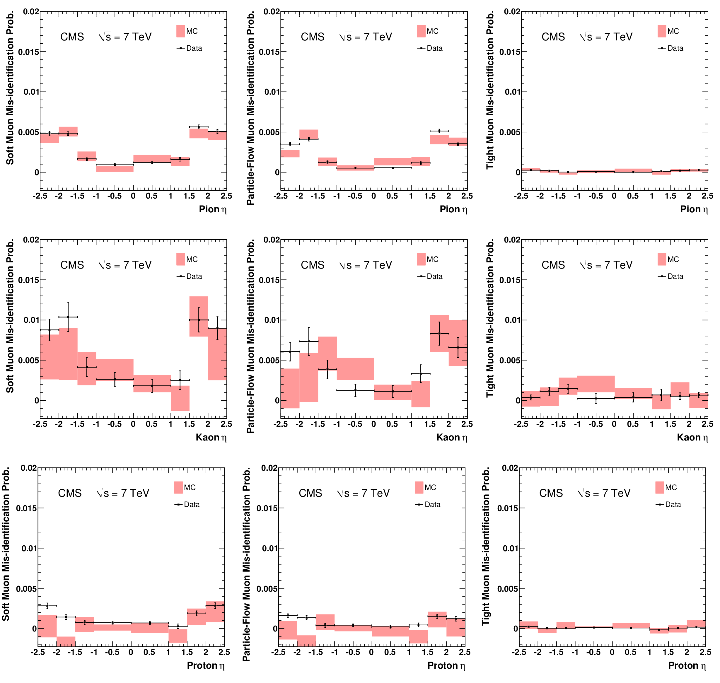
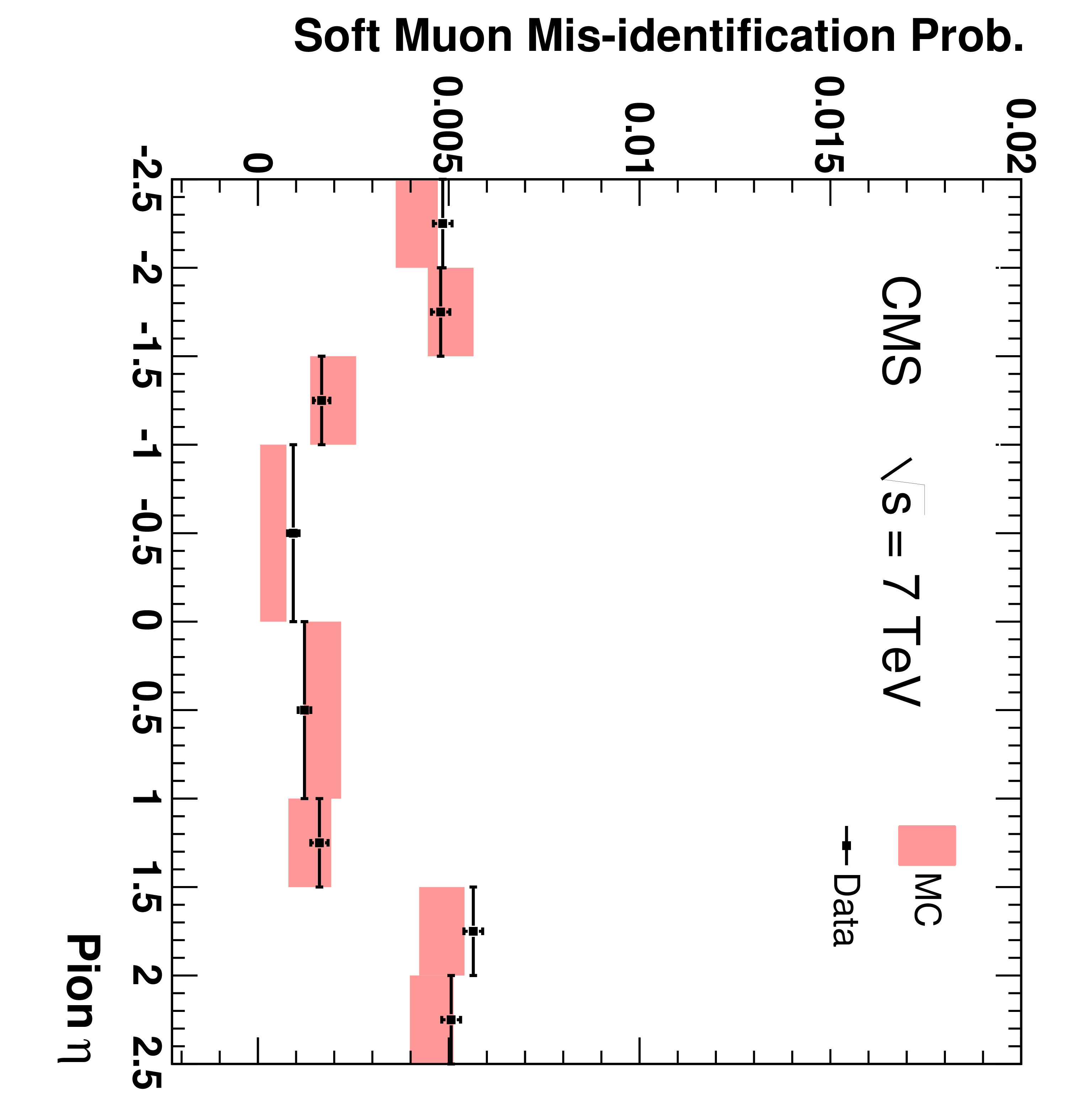
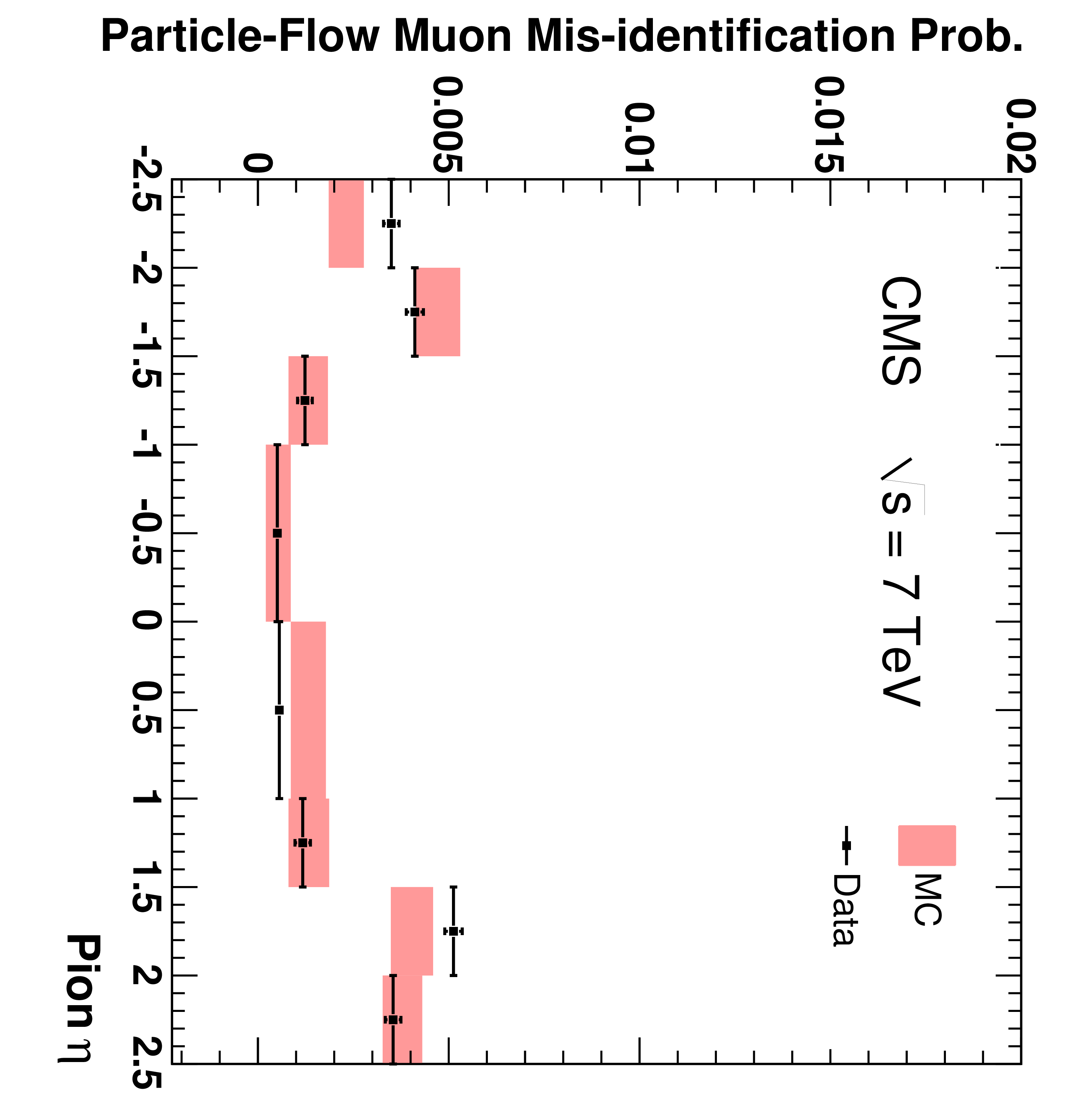
Figure 16:
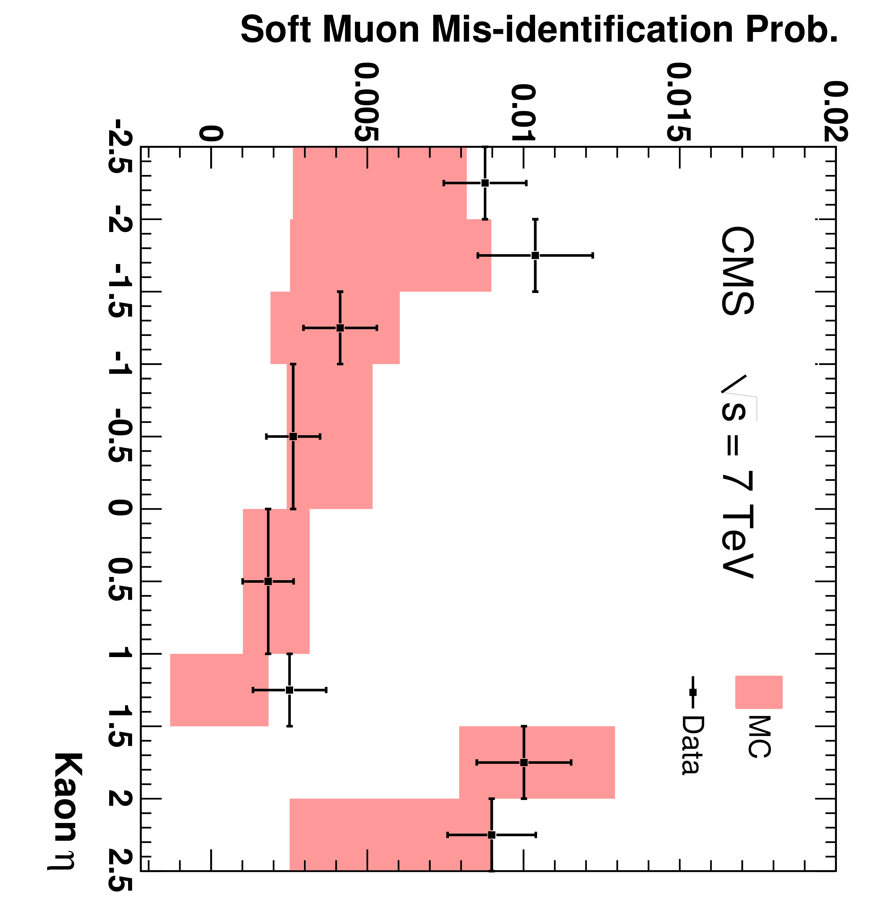
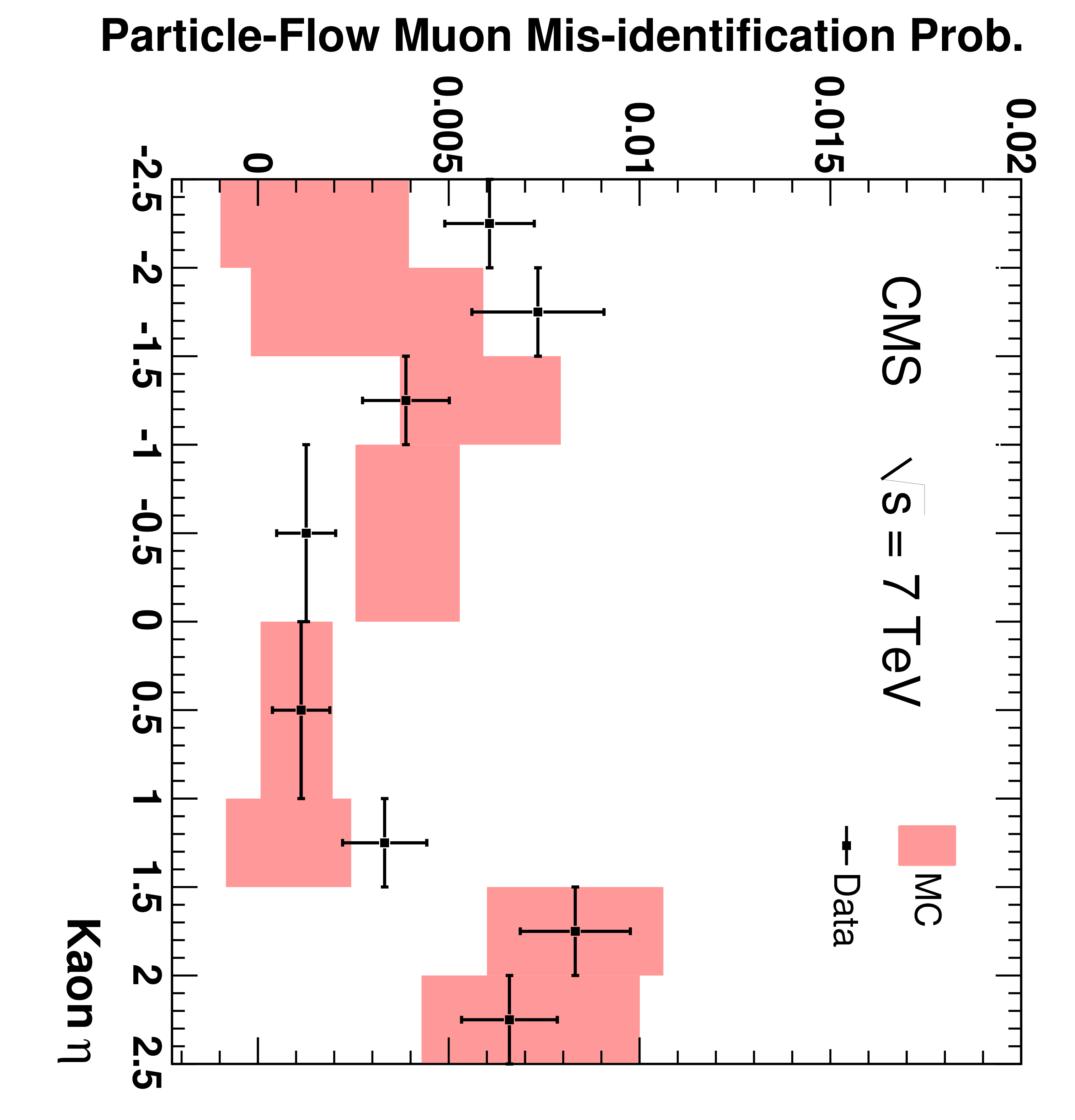
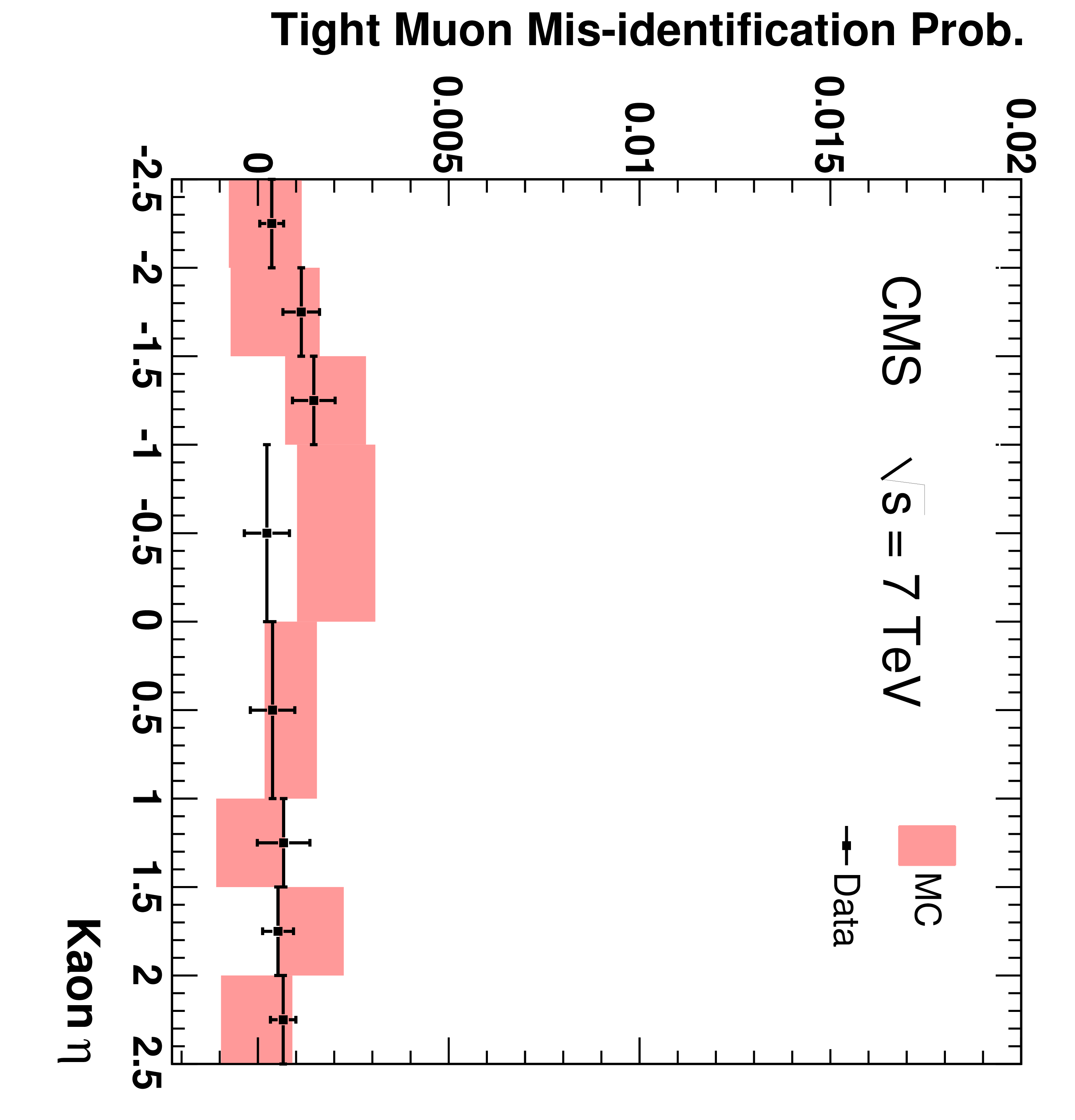
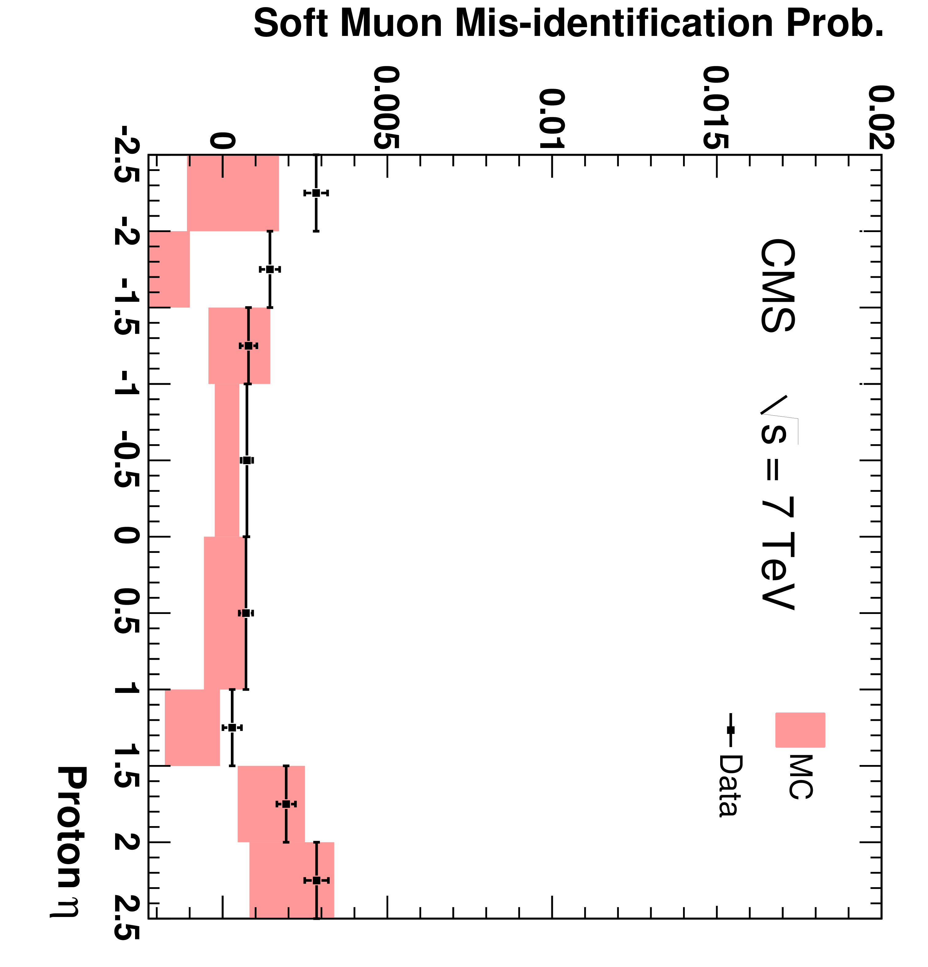
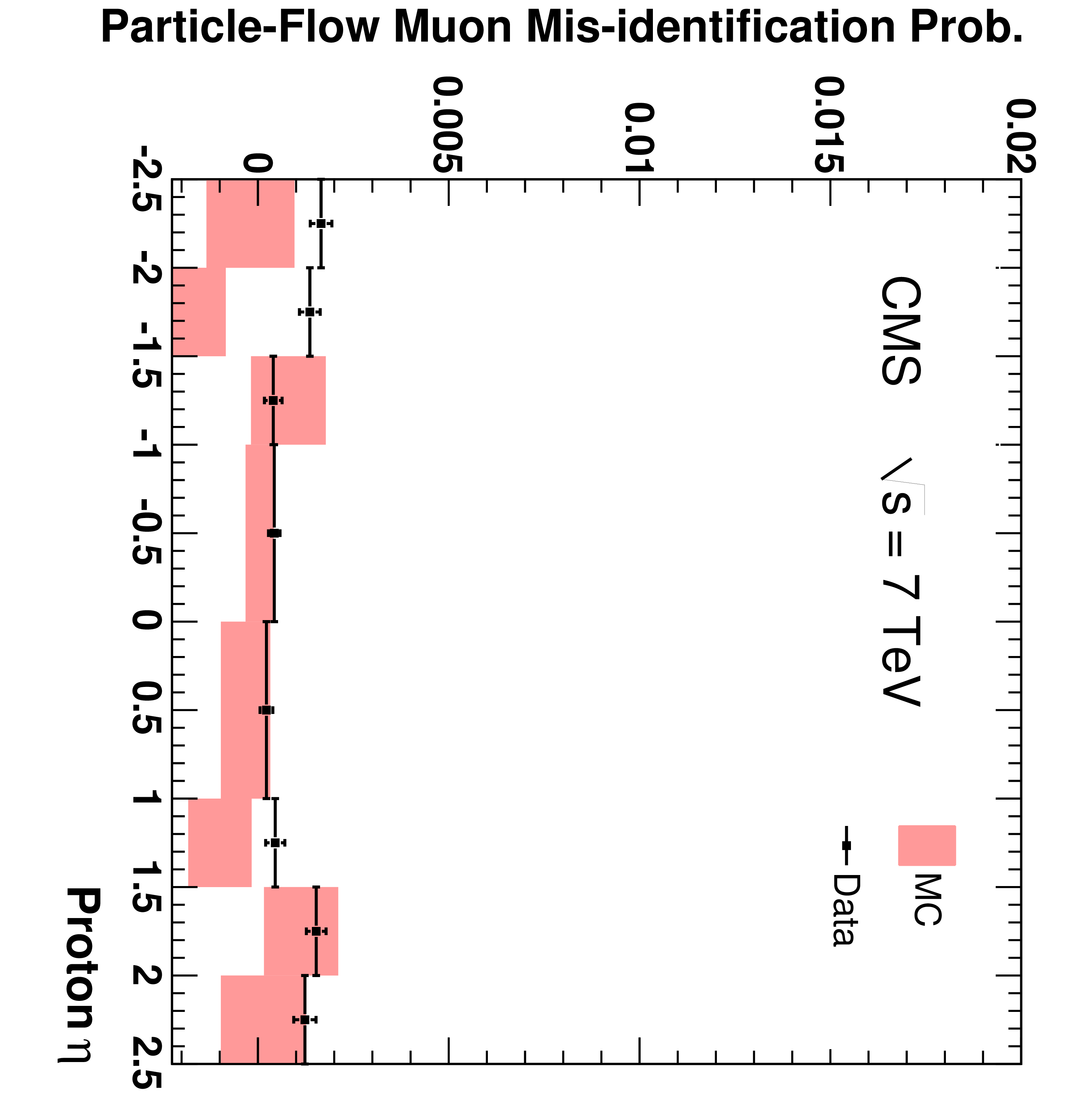
The fractions of pions (top), kaons (centre), and protons (bottom) that are misidentified as Soft Muons (left), Particle-Flow Muons (centre), or Tight Muons (right) as a function of pseudorapidity. Only particles with $p > $ 3 GeV/$c$ and $N_{\mathrm {Tracks}} < 4$ are included. The uncertainties indicated by the error bars (data) and shaded boxes (PYTHIA simulation) are statistical only. |
png pdf |
Figure 16-a:
The fractions of pions (top), kaons (centre), and protons (bottom) that are misidentified as Soft Muons (left), Particle-Flow Muons (centre), or Tight Muons (right) as a function of pseudorapidity. Only particles with $p > $ 3 GeV/$c$ and $N_{\mathrm {Tracks}} < 4$ are included. The uncertainties indicated by the error bars (data) and shaded boxes (PYTHIA simulation) are statistical only. |
png pdf |
Figure 16-b:
The fractions of pions (top), kaons (centre), and protons (bottom) that are misidentified as Soft Muons (left), Particle-Flow Muons (centre), or Tight Muons (right) as a function of pseudorapidity. Only particles with $p > $ 3 GeV/$c$ and $N_{\mathrm {Tracks}} < 4$ are included. The uncertainties indicated by the error bars (data) and shaded boxes (PYTHIA simulation) are statistical only. |

png pdf |
Figure 16-c:
The fractions of pions (top), kaons (centre), and protons (bottom) that are misidentified as Soft Muons (left), Particle-Flow Muons (centre), or Tight Muons (right) as a function of pseudorapidity. Only particles with $p > $ 3 GeV/$c$ and $N_{\mathrm {Tracks}} < 4$ are included. The uncertainties indicated by the error bars (data) and shaded boxes (PYTHIA simulation) are statistical only. |
png pdf |
Figure 16-d:
The fractions of pions (top), kaons (centre), and protons (bottom) that are misidentified as Soft Muons (left), Particle-Flow Muons (centre), or Tight Muons (right) as a function of pseudorapidity. Only particles with $p > $ 3 GeV/$c$ and $N_{\mathrm {Tracks}} < 4$ are included. The uncertainties indicated by the error bars (data) and shaded boxes (PYTHIA simulation) are statistical only. |
png pdf |
Figure 16-e:
The fractions of pions (top), kaons (centre), and protons (bottom) that are misidentified as Soft Muons (left), Particle-Flow Muons (centre), or Tight Muons (right) as a function of pseudorapidity. Only particles with $p > $ 3 GeV/$c$ and $N_{\mathrm {Tracks}} < 4$ are included. The uncertainties indicated by the error bars (data) and shaded boxes (PYTHIA simulation) are statistical only. |
png pdf |
Figure 16-f:
The fractions of pions (top), kaons (centre), and protons (bottom) that are misidentified as Soft Muons (left), Particle-Flow Muons (centre), or Tight Muons (right) as a function of pseudorapidity. Only particles with $p > $ 3 GeV/$c$ and $N_{\mathrm {Tracks}} < 4$ are included. The uncertainties indicated by the error bars (data) and shaded boxes (PYTHIA simulation) are statistical only. |
png pdf |
Figure 16-g:
The fractions of pions (top), kaons (centre), and protons (bottom) that are misidentified as Soft Muons (left), Particle-Flow Muons (centre), or Tight Muons (right) as a function of pseudorapidity. Only particles with $p > $ 3 GeV/$c$ and $N_{\mathrm {Tracks}} < 4$ are included. The uncertainties indicated by the error bars (data) and shaded boxes (PYTHIA simulation) are statistical only. |
png pdf |
Figure 16-h:
The fractions of pions (top), kaons (centre), and protons (bottom) that are misidentified as Soft Muons (left), Particle-Flow Muons (centre), or Tight Muons (right) as a function of pseudorapidity. Only particles with $p > $ 3 GeV/$c$ and $N_{\mathrm {Tracks}} < 4$ are included. The uncertainties indicated by the error bars (data) and shaded boxes (PYTHIA simulation) are statistical only. |

png pdf |
Figure 16-i:
The fractions of pions (top), kaons (centre), and protons (bottom) that are misidentified as Soft Muons (left), Particle-Flow Muons (centre), or Tight Muons (right) as a function of pseudorapidity. Only particles with $p > $ 3 GeV/$c$ and $N_{\mathrm {Tracks}} < 4$ are included. The uncertainties indicated by the error bars (data) and shaded boxes (PYTHIA simulation) are statistical only. |
png pdf |
Figure 17:
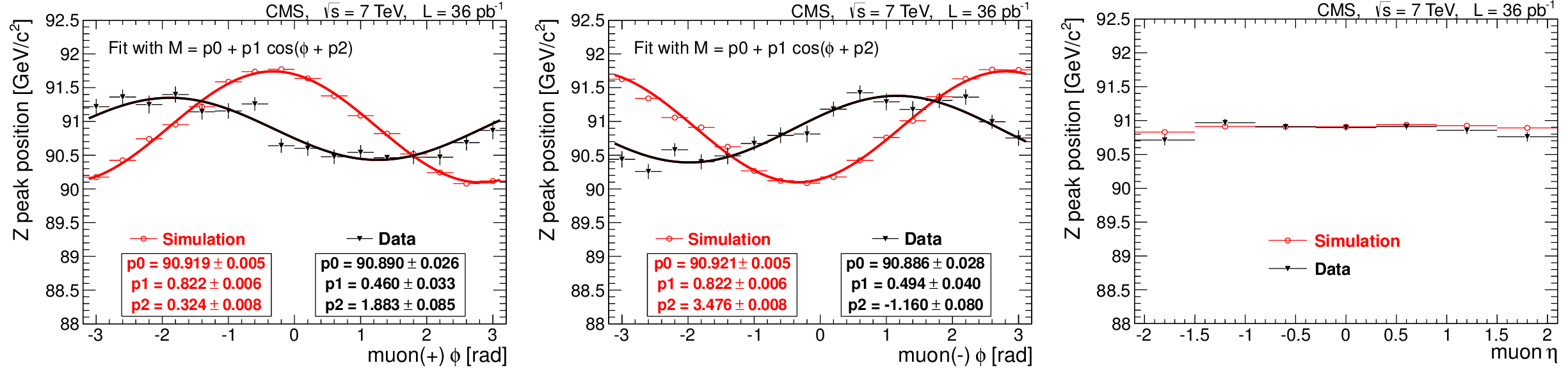
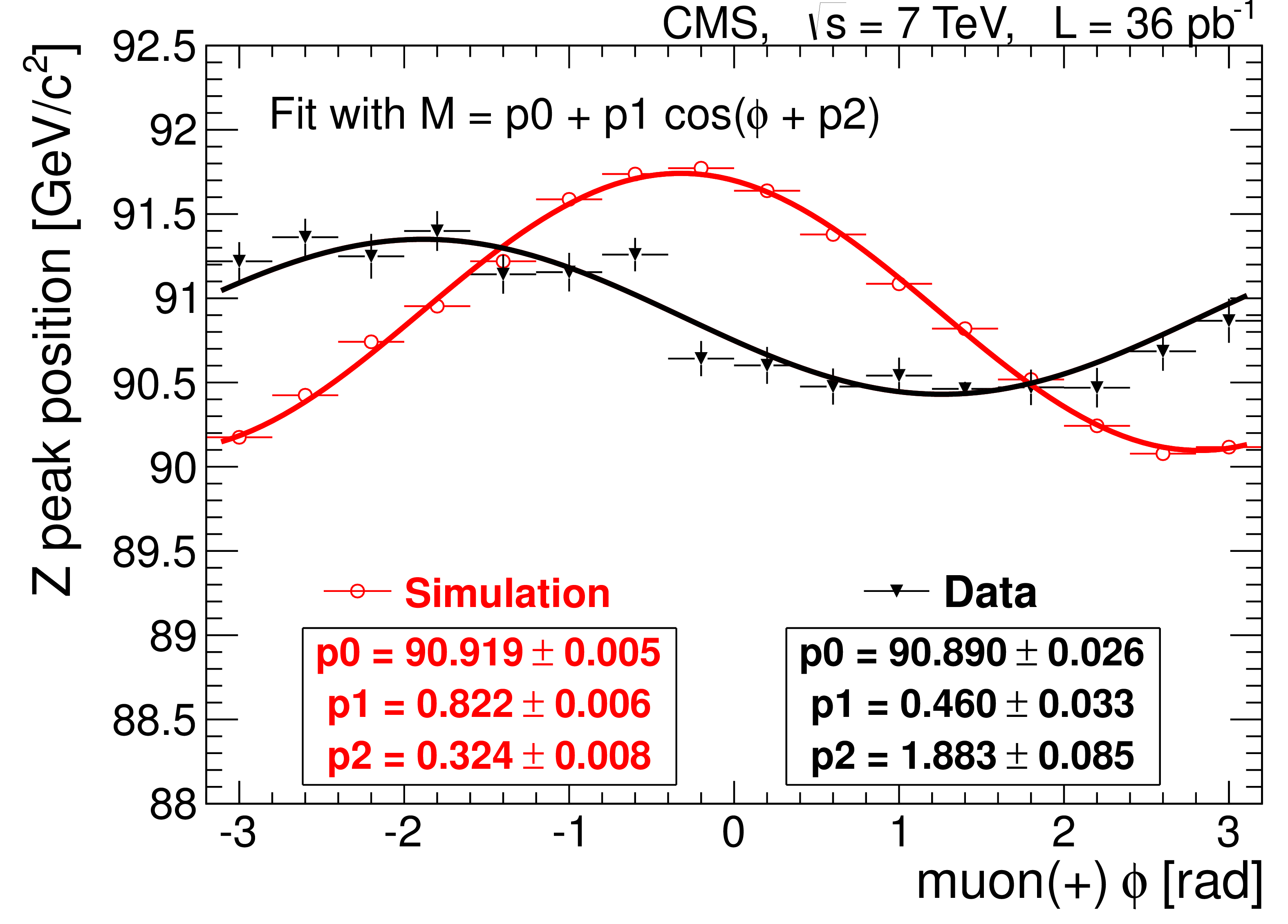
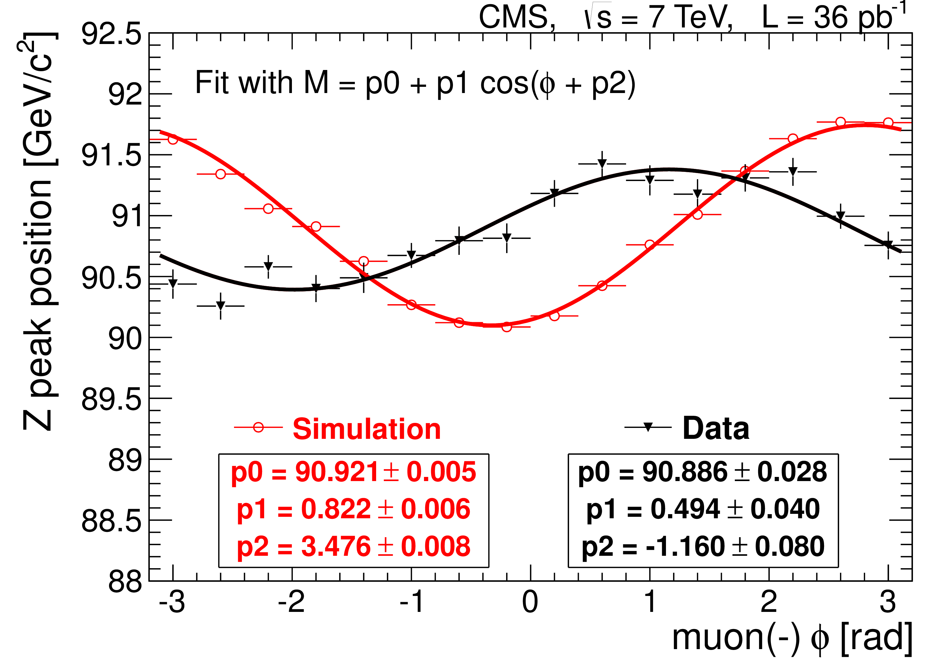
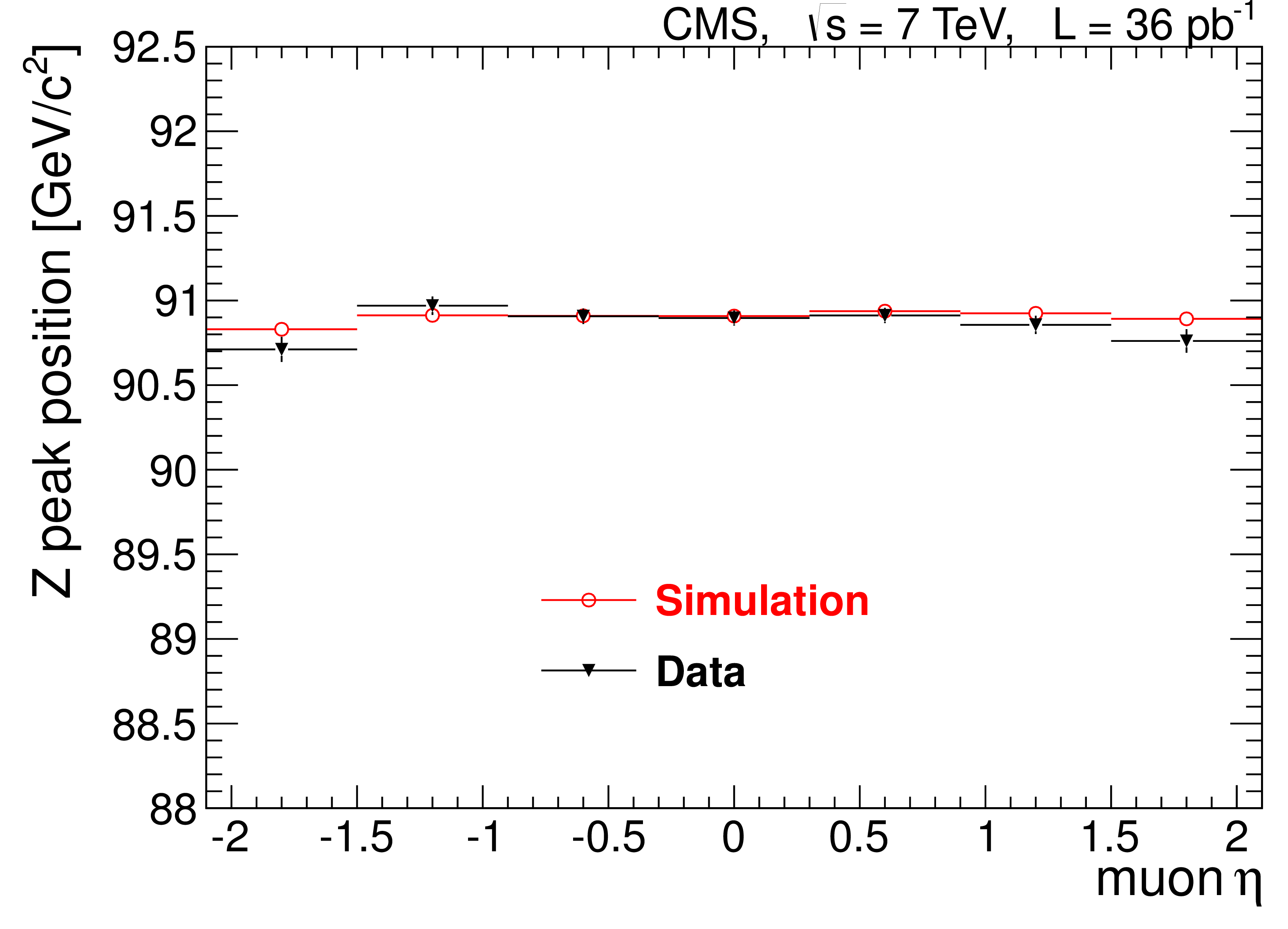
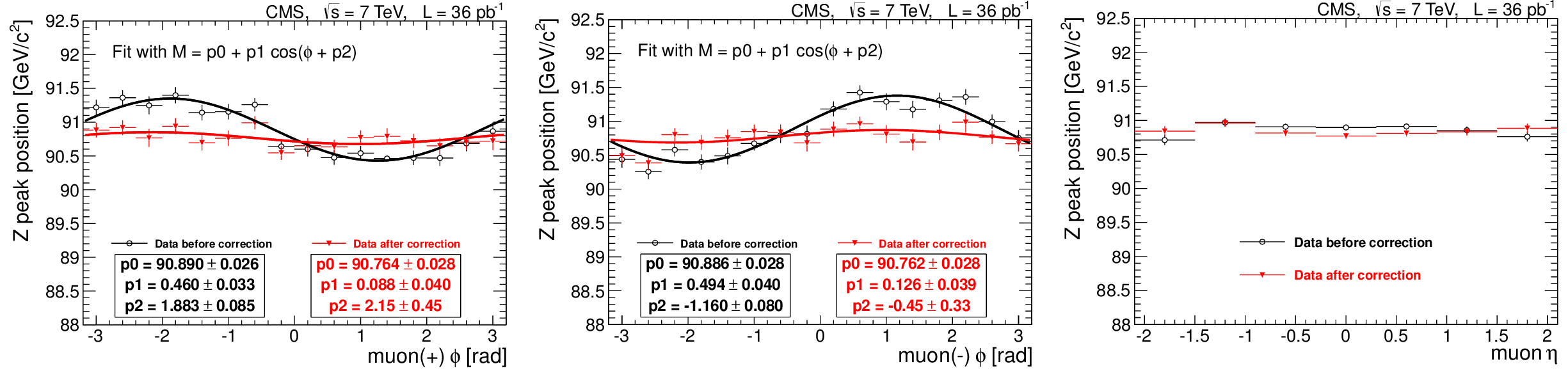
The position of the ${\mathrm{ Z } } $ peak reconstructed by the MuScleFit method as a function of muon $\phi $ for positively charged muons (left), $\phi $ for negatively charged muons (middle), and $\eta $ for muons of both charges (right). Results obtained from data (black triangles) are compared with those from simulation (red circles). The $\phi $ plots also show the results of sinusoidal fits; the values of the fit parameters are given in the text boxes below the labels. |
png pdf |
Figure 17-a:
The position of the ${\mathrm{ Z } } $ peak reconstructed by the MuScleFit method as a function of muon $\phi $ for positively charged muons (left), $\phi $ for negatively charged muons (middle), and $\eta $ for muons of both charges (right). Results obtained from data (black triangles) are compared with those from simulation (red circles). The $\phi $ plots also show the results of sinusoidal fits; the values of the fit parameters are given in the text boxes below the labels. |
png pdf |
Figure 17-b:
The position of the ${\mathrm{ Z } } $ peak reconstructed by the MuScleFit method as a function of muon $\phi $ for positively charged muons (left), $\phi $ for negatively charged muons (middle), and $\eta $ for muons of both charges (right). Results obtained from data (black triangles) are compared with those from simulation (red circles). The $\phi $ plots also show the results of sinusoidal fits; the values of the fit parameters are given in the text boxes below the labels. |
png pdf |
Figure 17-c:
The position of the ${\mathrm{ Z } } $ peak reconstructed by the MuScleFit method as a function of muon $\phi $ for positively charged muons (left), $\phi $ for negatively charged muons (middle), and $\eta $ for muons of both charges (right). Results obtained from data (black triangles) are compared with those from simulation (red circles). The $\phi $ plots also show the results of sinusoidal fits; the values of the fit parameters are given in the text boxes below the labels. |
png pdf |
Figure 18:
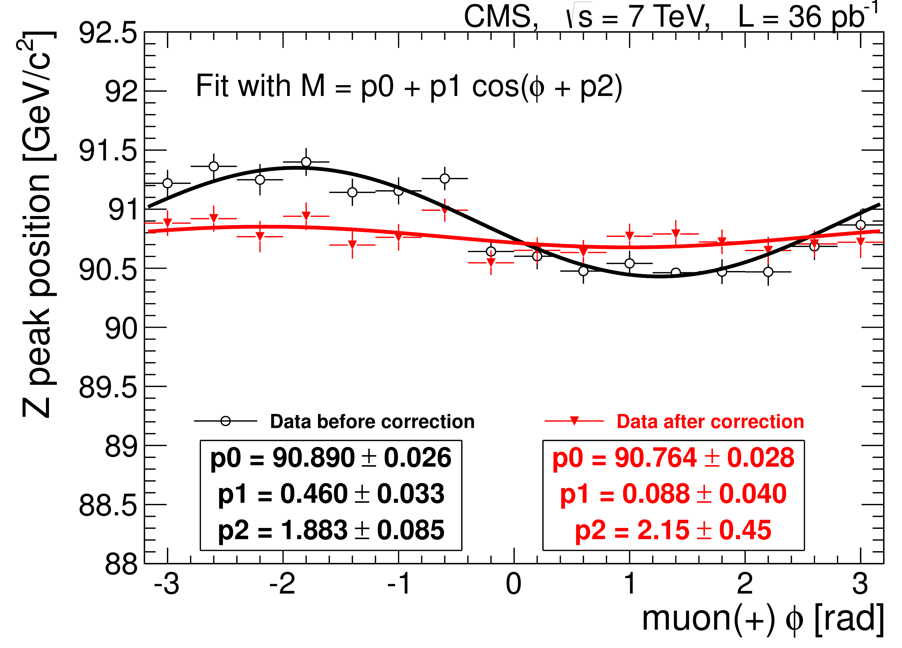
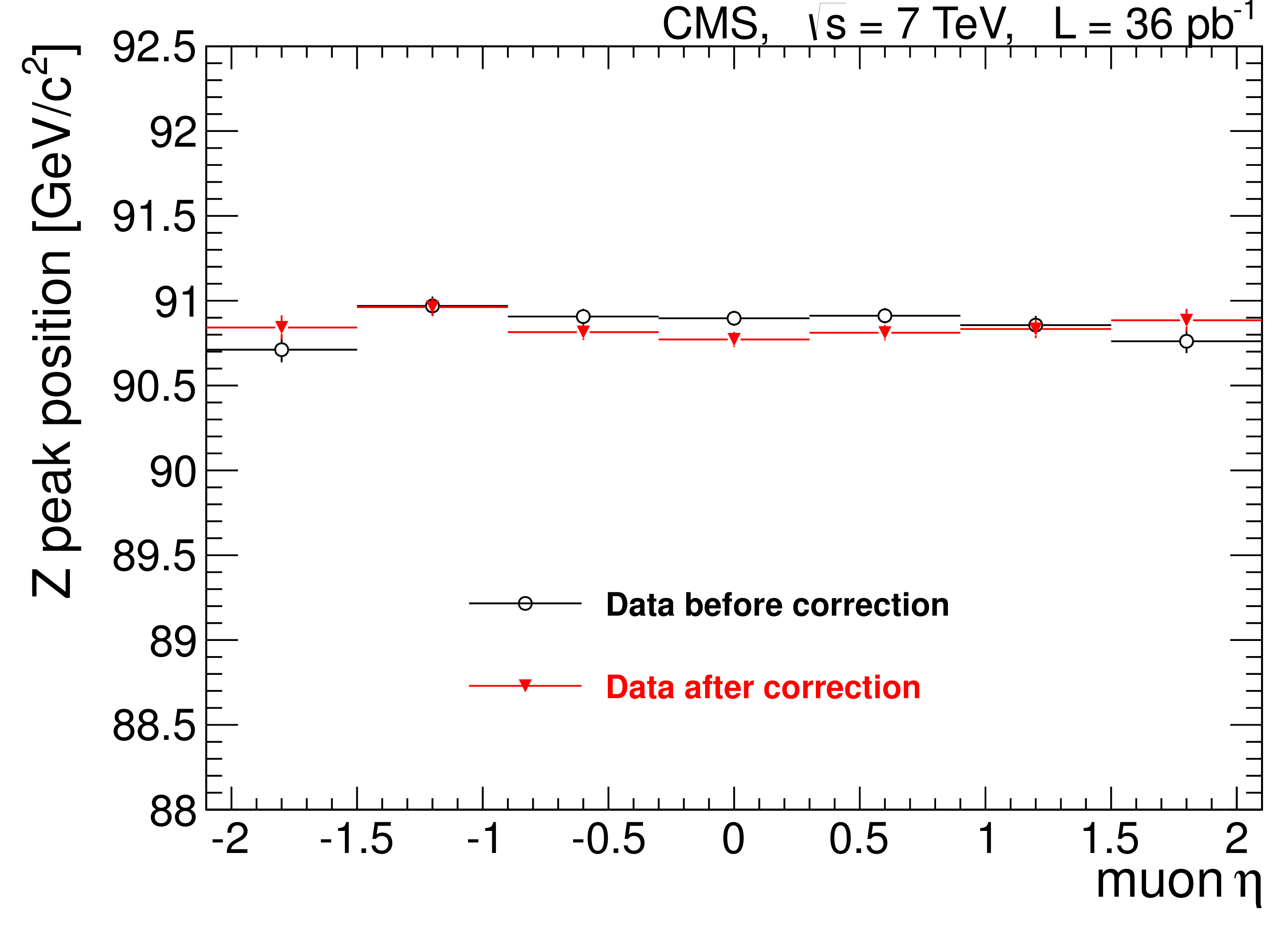
The position of the ${\mathrm{ Z } } $ peak in data as a function of muon $\phi $ for positively charged muons (left), $\phi $ for negatively charged muons (middle), and $\eta $ for muons of both charges (right) before (black circles) and after (red triangles) the MuScleFit calibration. The $\phi $ plots also show the results of sinusoidal fits; the values of the fit parameters are given in the text boxes below the labels. |
png pdf |
Figure 18-a:
The position of the ${\mathrm{ Z } } $ peak in data as a function of muon $\phi $ for positively charged muons (left), $\phi $ for negatively charged muons (middle), and $\eta $ for muons of both charges (right) before (black circles) and after (red triangles) the MuScleFit calibration. The $\phi $ plots also show the results of sinusoidal fits; the values of the fit parameters are given in the text boxes below the labels. |

png pdf |
Figure 18-b:
The position of the ${\mathrm{ Z } } $ peak in data as a function of muon $\phi $ for positively charged muons (left), $\phi $ for negatively charged muons (middle), and $\eta $ for muons of both charges (right) before (black circles) and after (red triangles) the MuScleFit calibration. The $\phi $ plots also show the results of sinusoidal fits; the values of the fit parameters are given in the text boxes below the labels. |
png pdf |
Figure 18-c:
The position of the ${\mathrm{ Z } } $ peak in data as a function of muon $\phi $ for positively charged muons (left), $\phi $ for negatively charged muons (middle), and $\eta $ for muons of both charges (right) before (black circles) and after (red triangles) the MuScleFit calibration. The $\phi $ plots also show the results of sinusoidal fits; the values of the fit parameters are given in the text boxes below the labels. |
png pdf |
Figure 19:
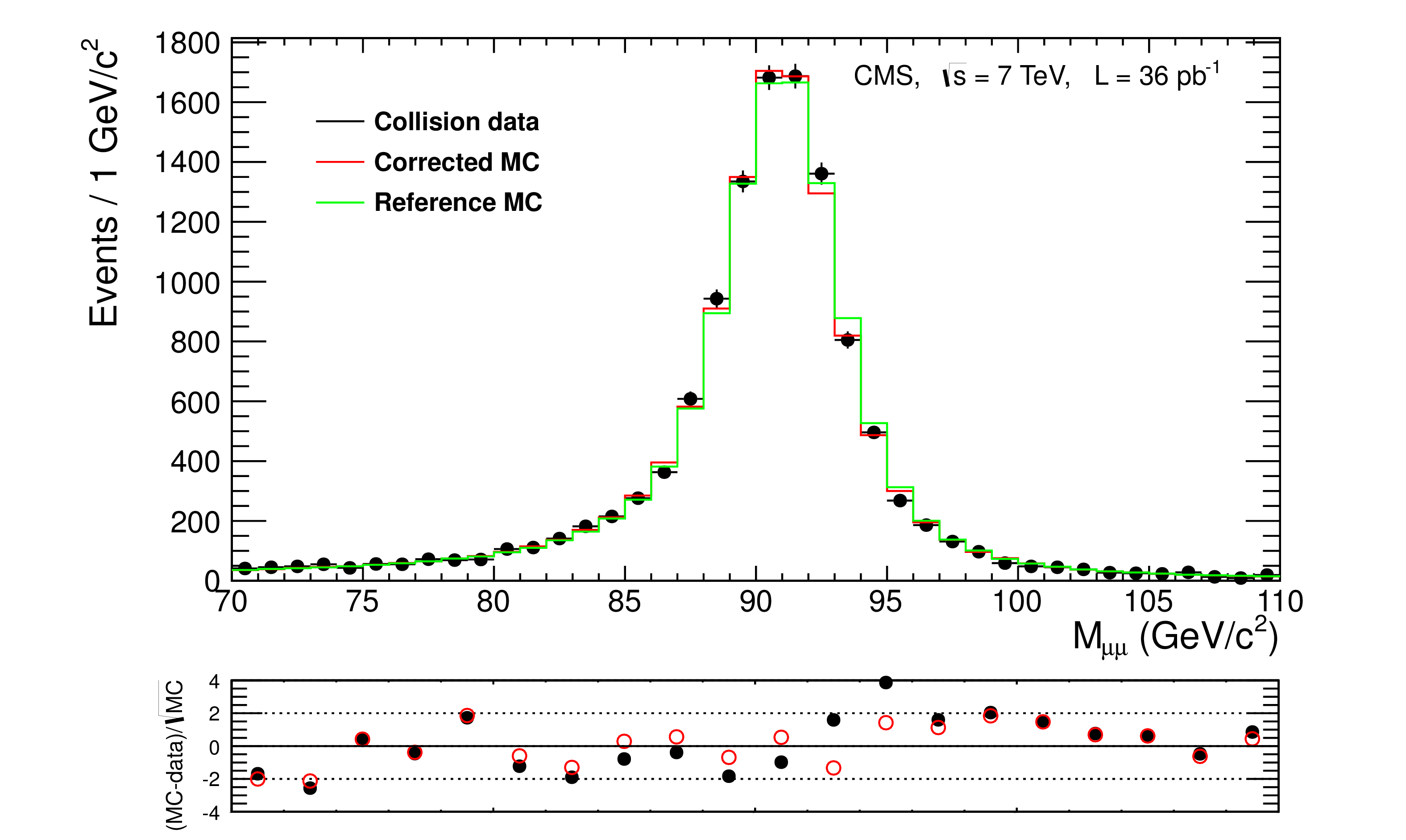
Top: distributions of the dimuon invariant mass for the selected $ {\mathrm {Z}}\to \mu ^+\mu ^-$ candidates in data (points with error bars) and in simulation without (``reference MC'') and with (``corrected MC'') corrections from SIDRA applied. Bottom: bin-by-bin difference (rebinned for clarity) between the simulation and the data, divided by the expected statistical uncertainty, for MC samples without (filled black circles) and with (open red circles) the SIDRA corrections. The uncertainties are statistical only. |
png pdf |
Figure 20:
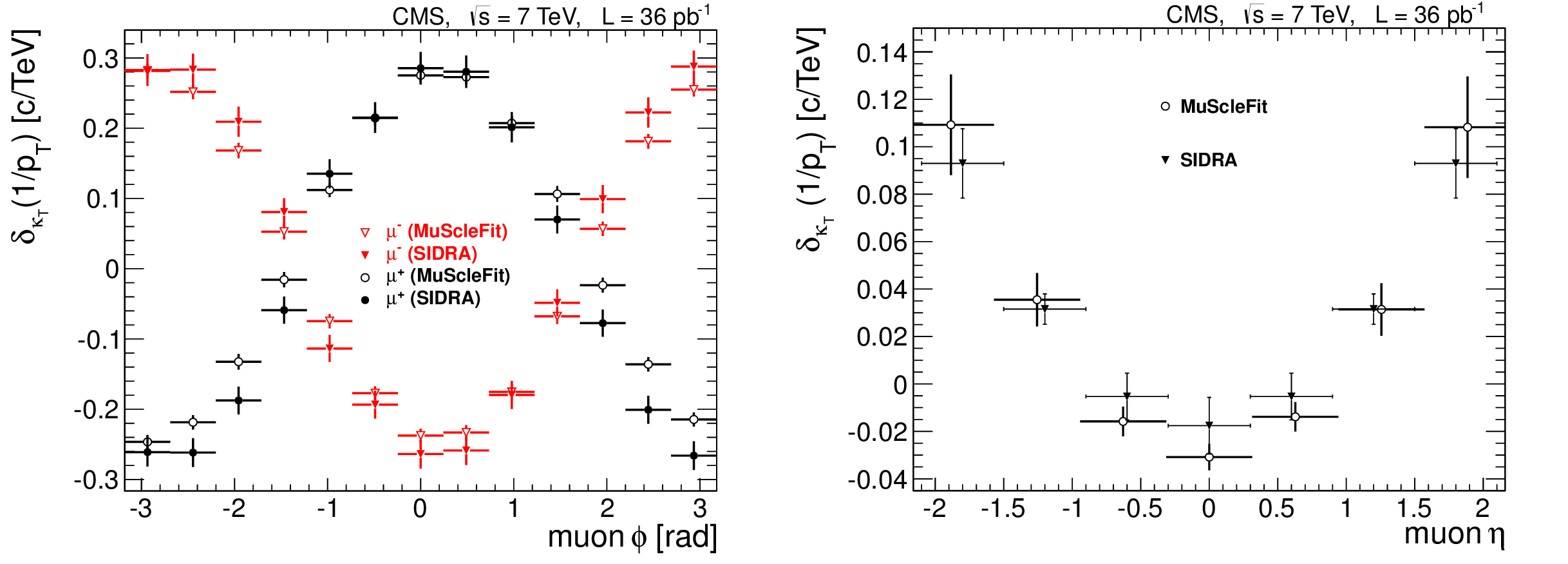
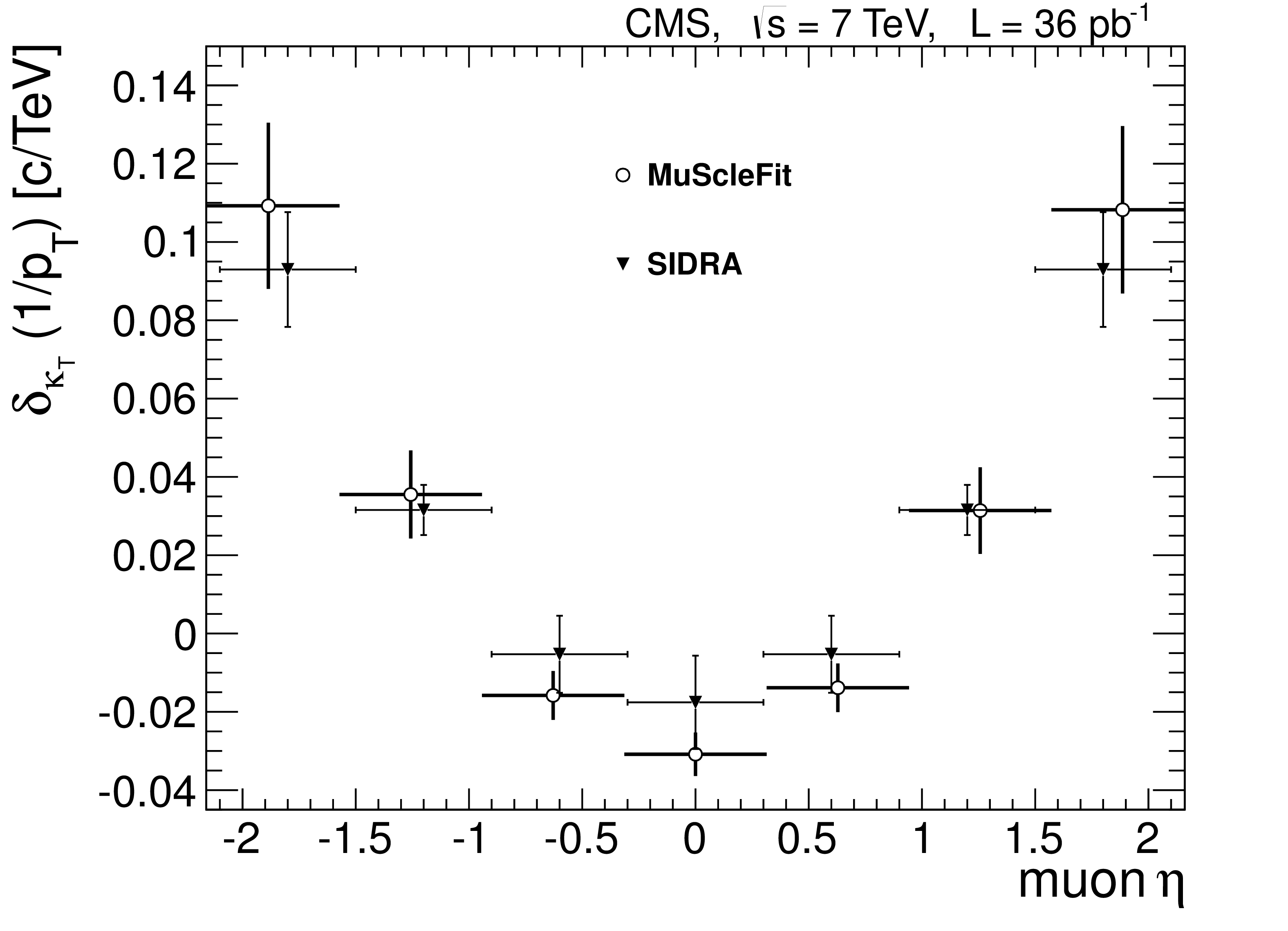
Comparison of the differences between muon momentum scale in data and that in the simulation obtained with the SIDRA and MuScleFit methods as a function of the azimuthal angle for positive and negative muons (left) and pseudorapidity (right). Only statistical uncertainties are shown. |

png pdf |
Figure 20-a:
Comparison of the differences between muon momentum scale in data and that in the simulation obtained with the SIDRA and MuScleFit methods as a function of the azimuthal angle for positive and negative muons (left) and pseudorapidity (right). Only statistical uncertainties are shown. |
png pdf |
Figure 20-b:
Comparison of the differences between muon momentum scale in data and that in the simulation obtained with the SIDRA and MuScleFit methods as a function of the azimuthal angle for positive and negative muons (left) and pseudorapidity (right). Only statistical uncertainties are shown. |

png pdf |
Figure 21:
Relative transverse momentum resolution $\sigma ( {p_{\mathrm {T}}} )/ {p_{\mathrm {T}}} $ in data and simulation measured by applying the MuScleFit and SIDRA methods to muons produced in the decays of ${\mathrm{ Z } } $ bosons and passing the Tight Muon selection. The thin line shows the result of MuScleFit on data, with the grey band representing the overall (statistical and systematic) 1$\sigma $ uncertainty of the measurement. The circles are the result of MuScleFit on simulation. The downward-pointing and upward-pointing triangles are the results from SIDRA obtained on data and simulation, respectively; the resolution in simulation was evaluated by comparing the reconstructed and ``true'' $ {p_{\mathrm {T}}} $ once the reconstructed $ {p_{\mathrm {T}}} $ was corrected for $\phi $-dependent biases. The uncertainties for SIDRA are statistical only and are smaller than the marker size. |
png pdf |
Figure 22:
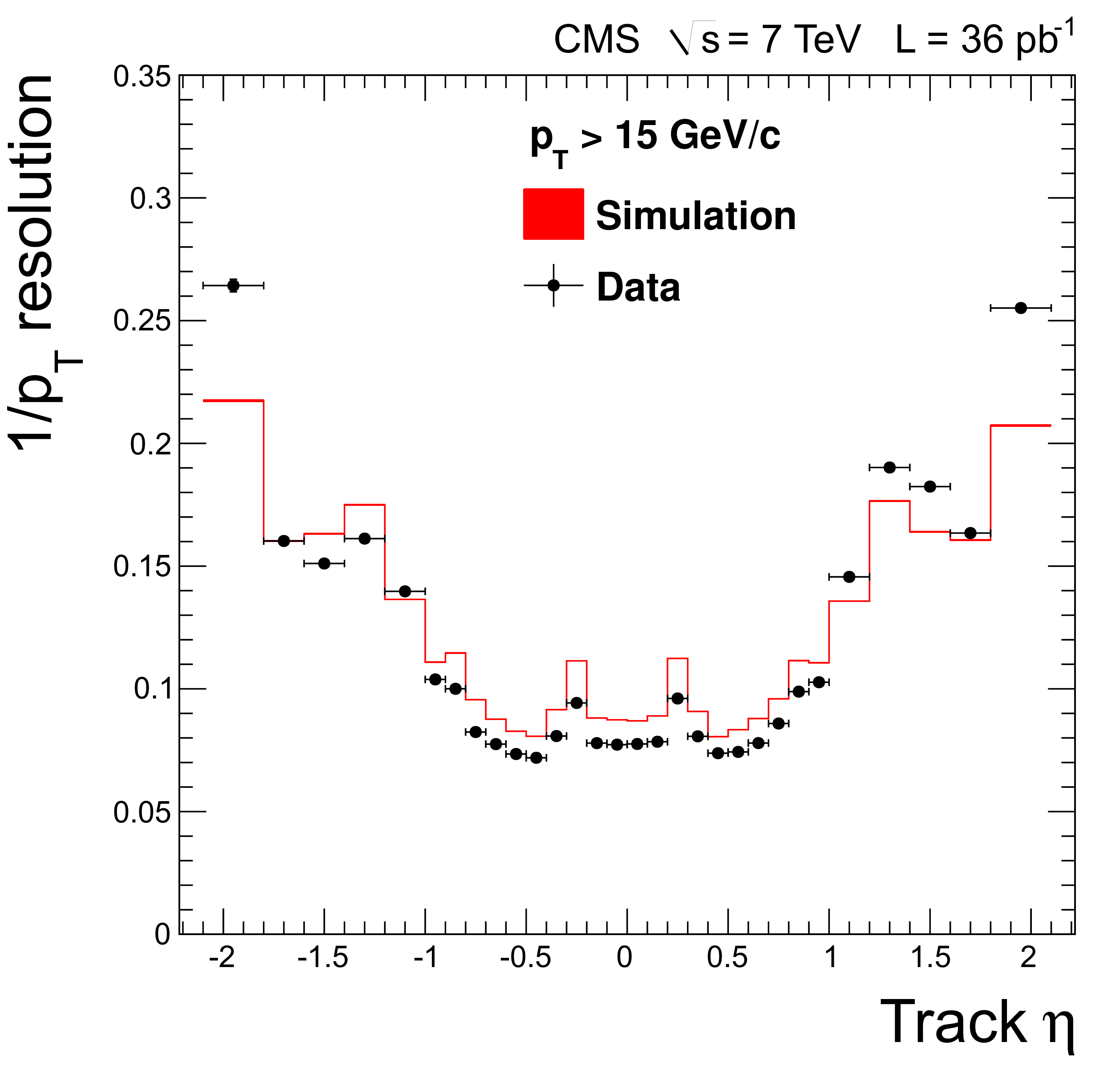
The $1/ {p_{\mathrm {T}}} $ resolution of standalone-muon tracks with respect to tracker tracks, as a function of $\eta $ of the tracker track for muons with $ {p_{\mathrm {T}}} > $ 15 GeV/$c$. Resolution is estimated as the $\sigma $ of a Gaussian fit to $R_{\mathrm {sta}}(1/ {p_{\mathrm {T}}} )$ defined in Eq.(\ref {eq:staResolData}). |
png pdf |
Figure 23:
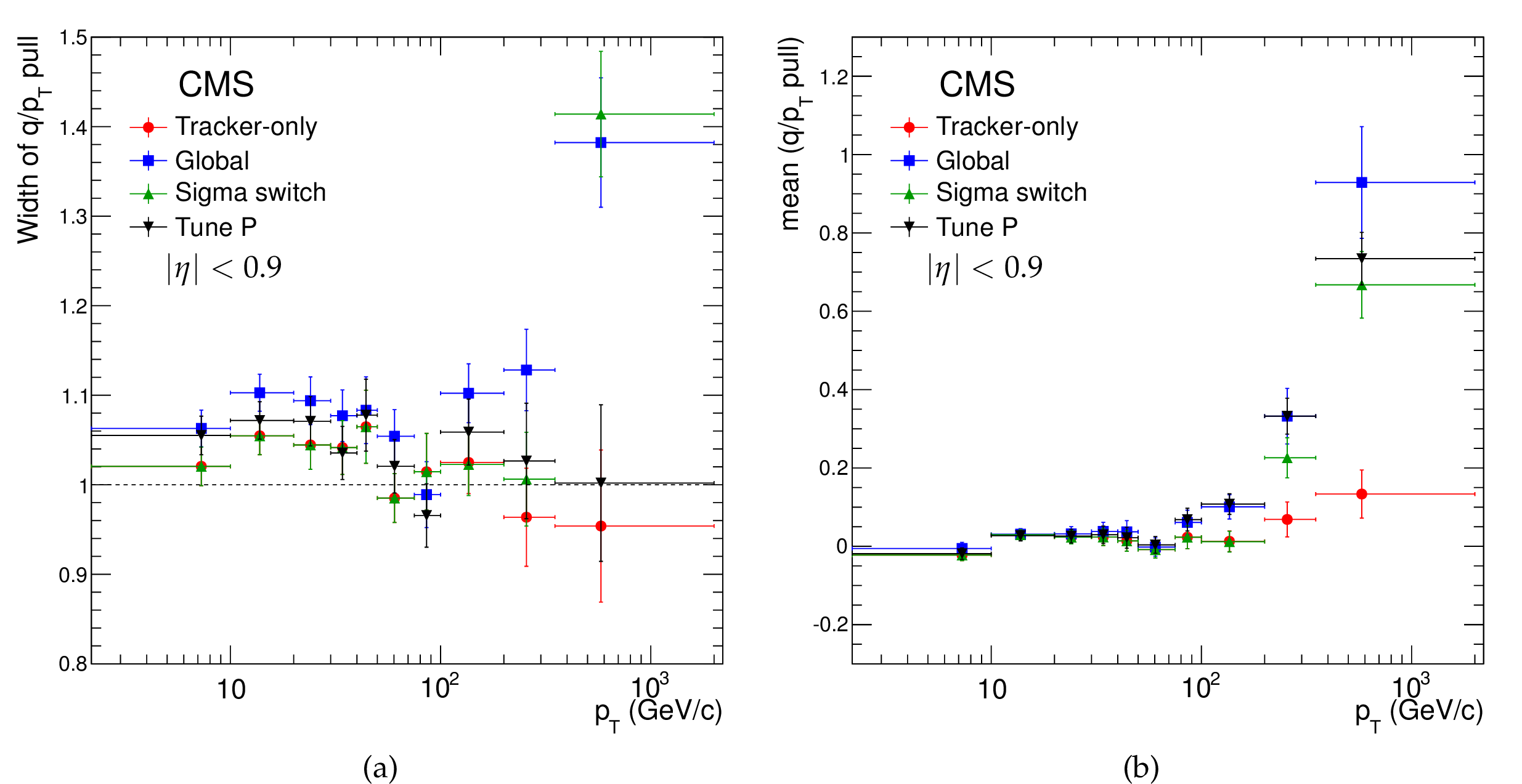
(a) Widths of Gaussian fits to the distributions of the muon $q/ {p_{\mathrm {T}}} $ pulls for the tracker-only and global fits, and for the output of the sigma-switch and Tune P algorithms, as a function of the $ {p_{\mathrm {T}}} $ of the muon; (b) the means of the same distributions. |

png pdf |
Figure 23-a:
(a) Widths of Gaussian fits to the distributions of the muon $q/ {p_{\mathrm {T}}} $ pulls for the tracker-only and global fits, and for the output of the sigma-switch and Tune P algorithms, as a function of the $ {p_{\mathrm {T}}} $ of the muon; (b) the means of the same distributions. |

png pdf |
Figure 23-b:
(a) Widths of Gaussian fits to the distributions of the muon $q/ {p_{\mathrm {T}}} $ pulls for the tracker-only and global fits, and for the output of the sigma-switch and Tune P algorithms, as a function of the $ {p_{\mathrm {T}}} $ of the muon; (b) the means of the same distributions. |
png pdf |
Figure 24:
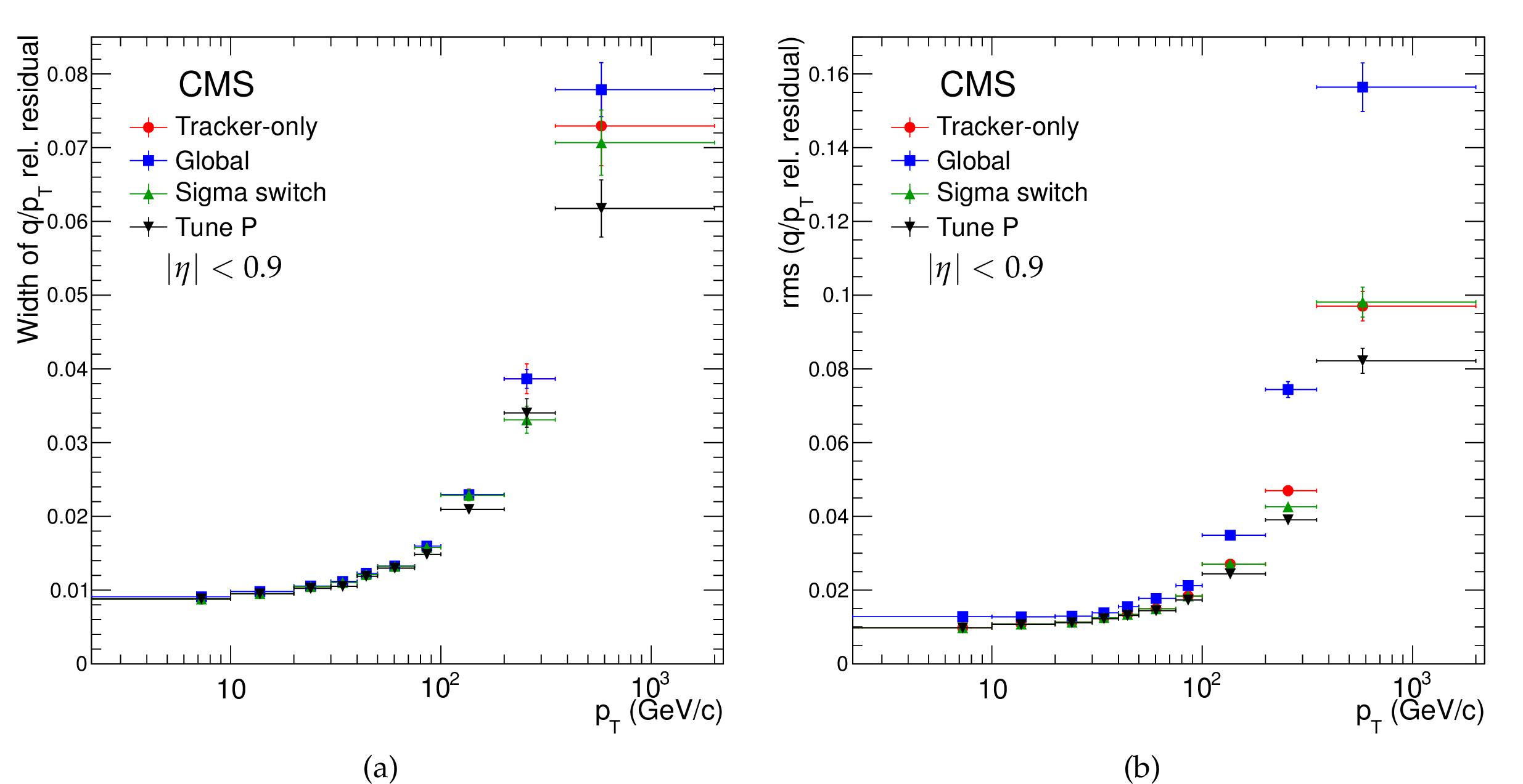
(a) Widths of Gaussian fits of the distributions of the muon $q/ {p_{\mathrm {T}}} $ relative residuals for the tracker-only and global fits, and for the output of the sigma-switch and Tune P algorithms, as a function of the $ {p_{\mathrm {T}}} $ of the muon; (b) sample RMS values (truncated at $\pm$1) of the same distributions. |

png pdf |
Figure 24-a:
(a) Widths of Gaussian fits of the distributions of the muon $q/ {p_{\mathrm {T}}} $ relative residuals for the tracker-only and global fits, and for the output of the sigma-switch and Tune P algorithms, as a function of the $ {p_{\mathrm {T}}} $ of the muon; (b) sample RMS values (truncated at $\pm$1) of the same distributions. |

png pdf |
Figure 24-b:
(a) Widths of Gaussian fits of the distributions of the muon $q/ {p_{\mathrm {T}}} $ relative residuals for the tracker-only and global fits, and for the output of the sigma-switch and Tune P algorithms, as a function of the $ {p_{\mathrm {T}}} $ of the muon; (b) sample RMS values (truncated at $\pm$1) of the same distributions. |
png pdf |
Figure 25:
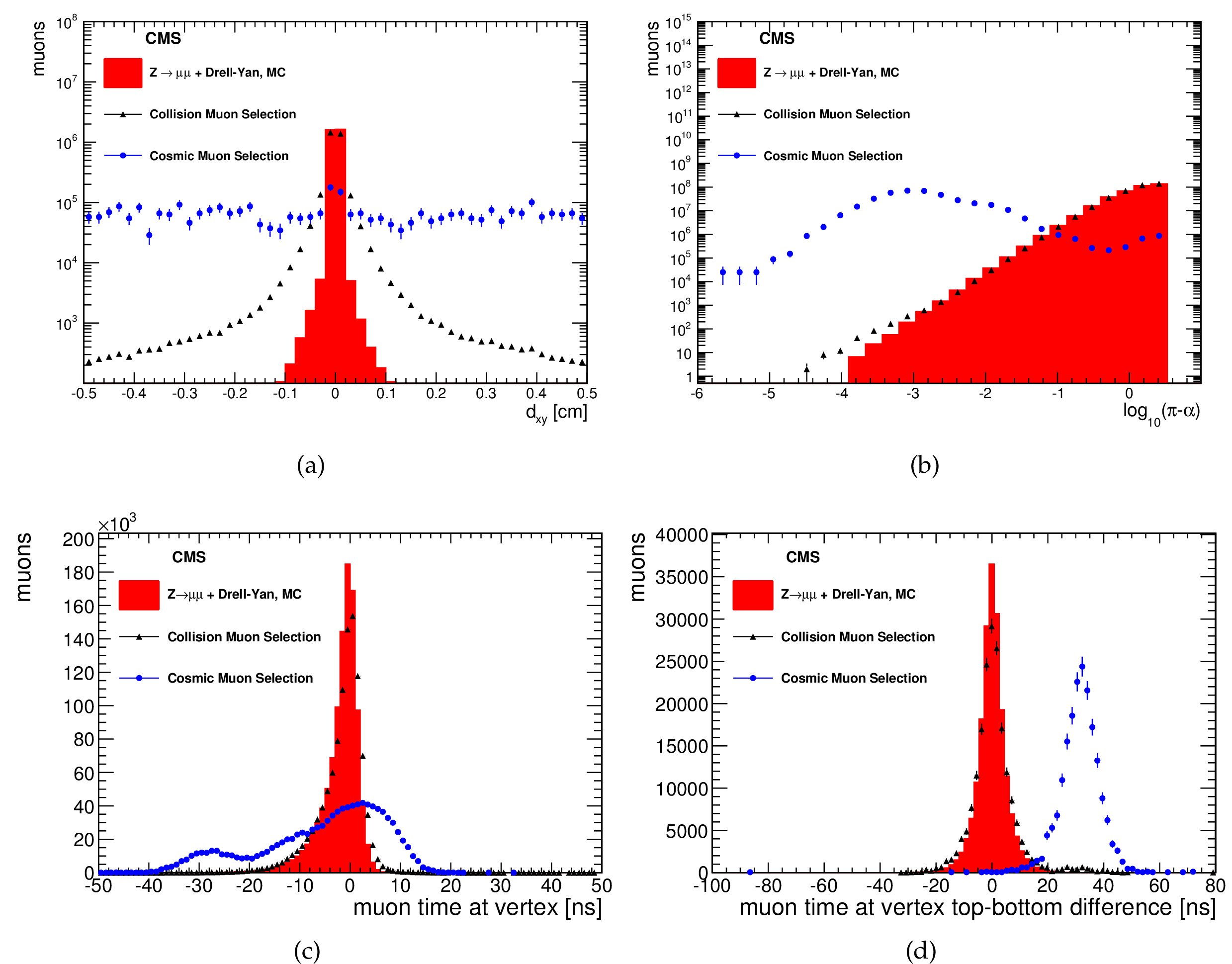
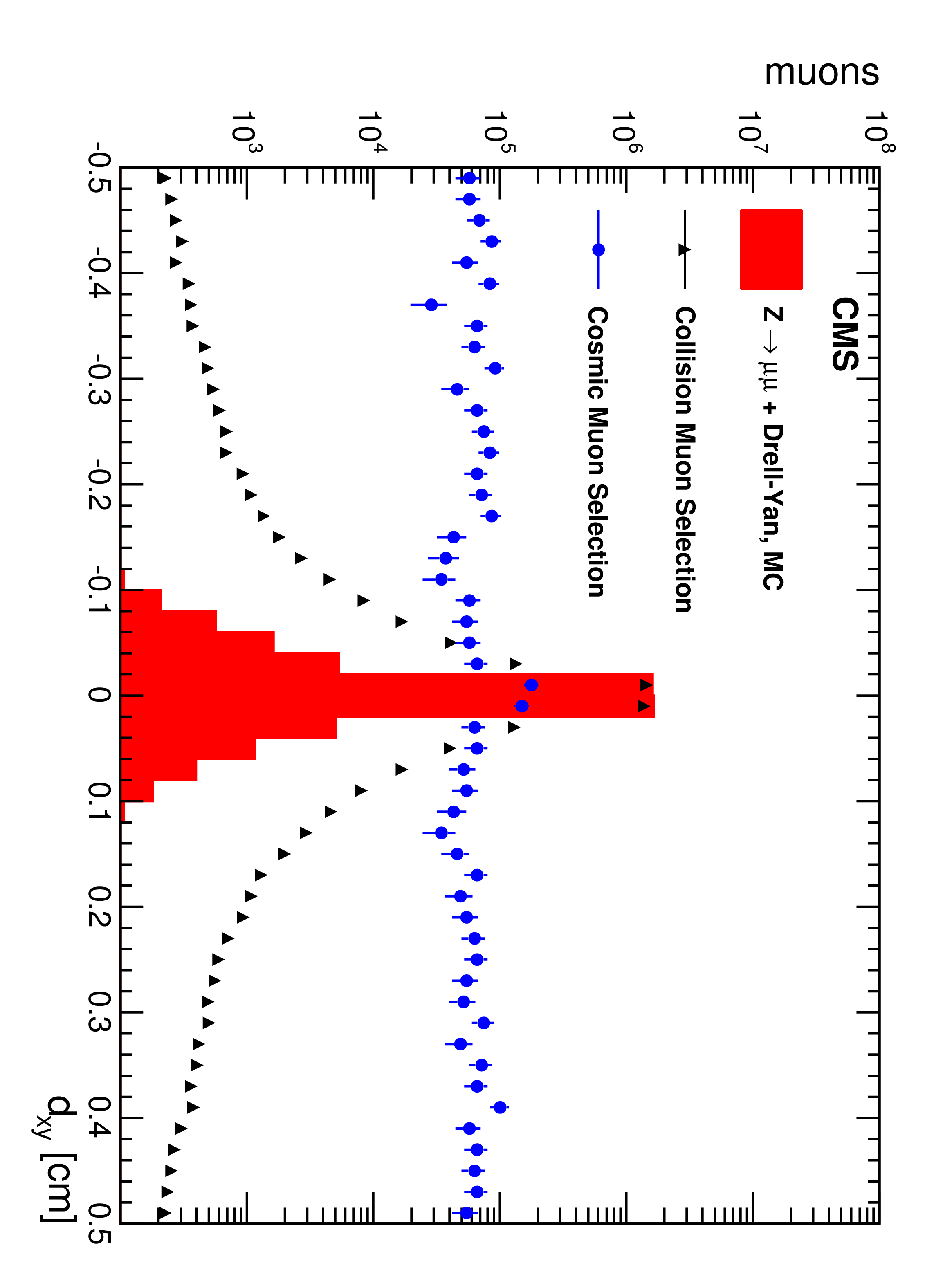
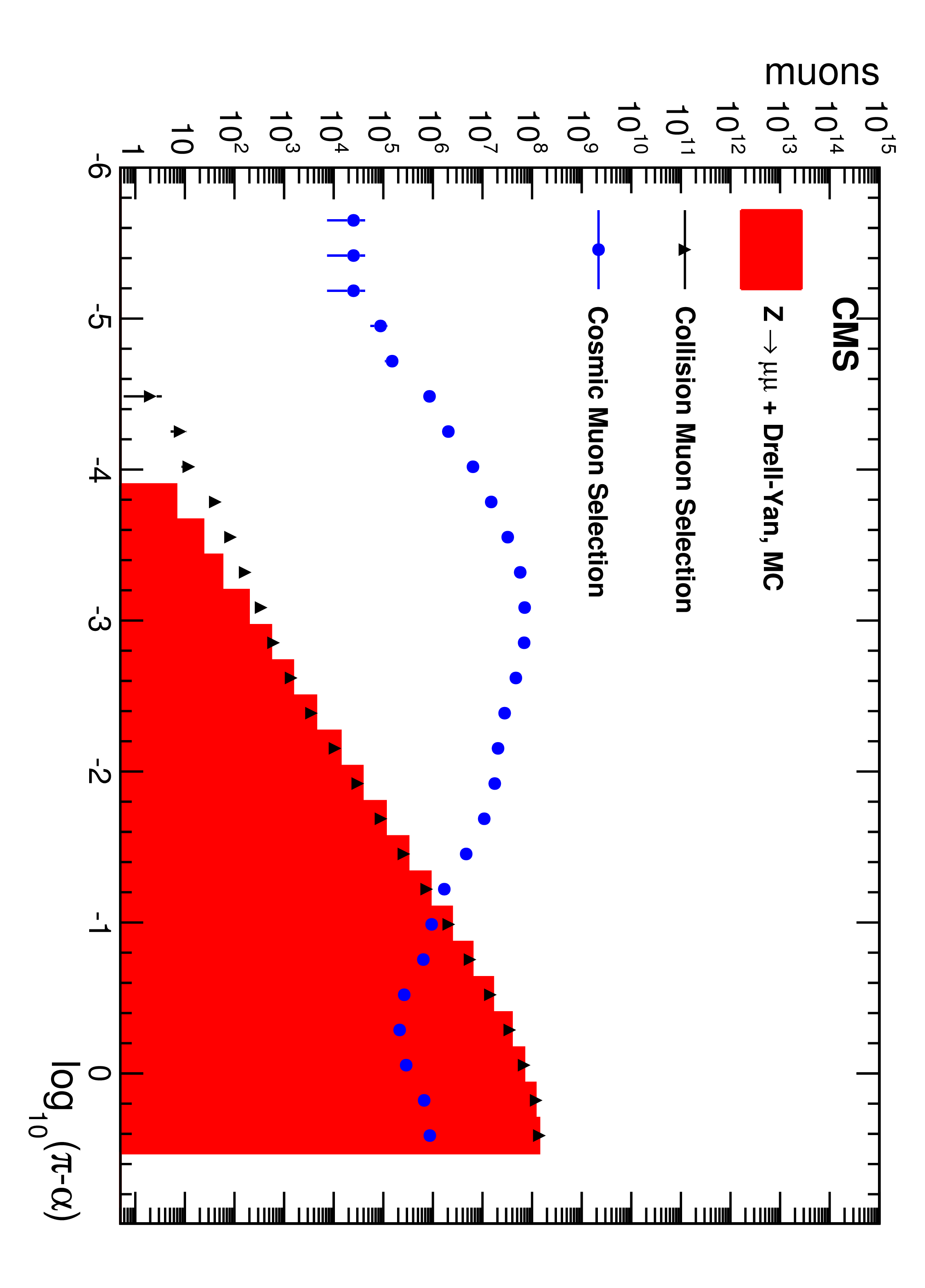
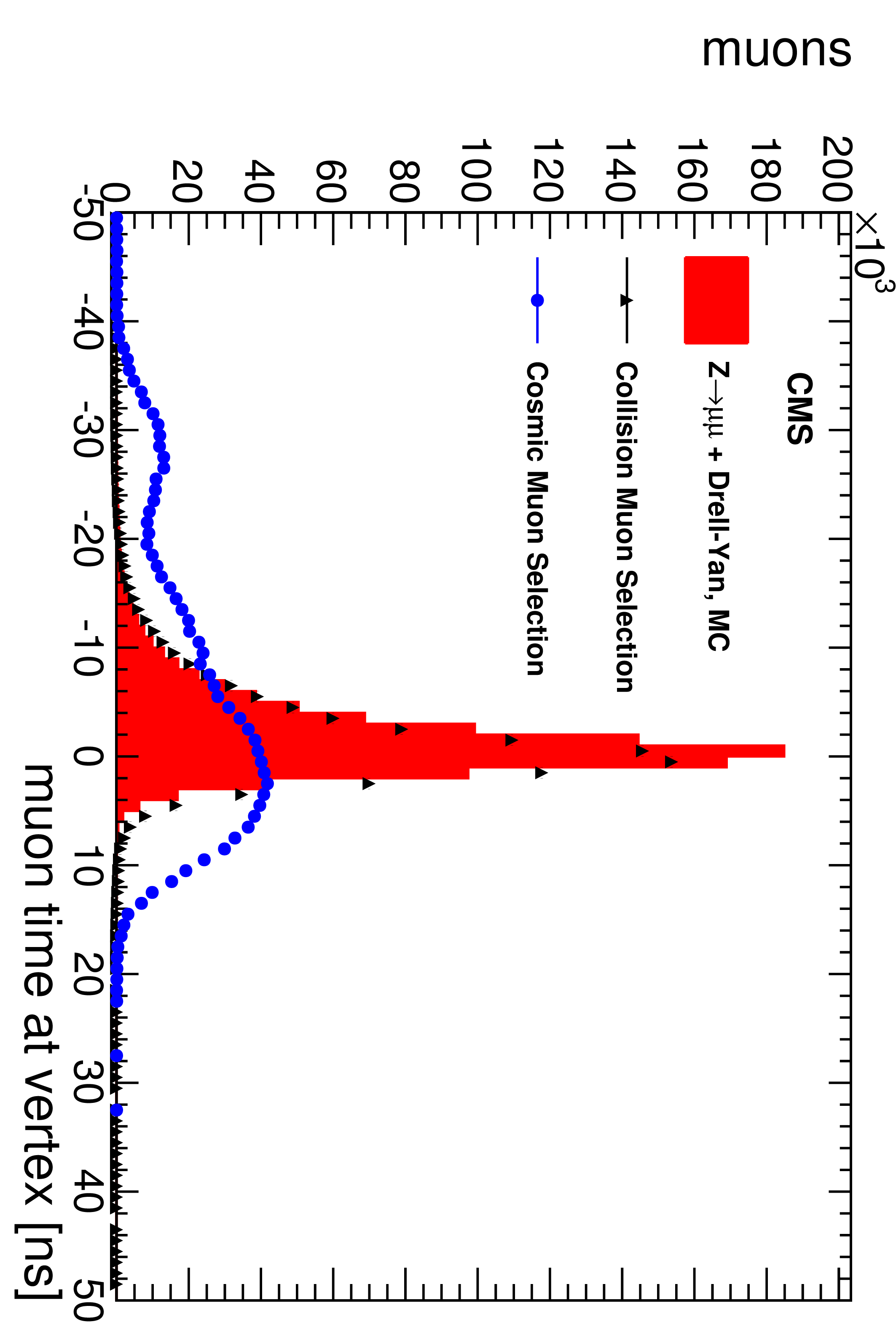
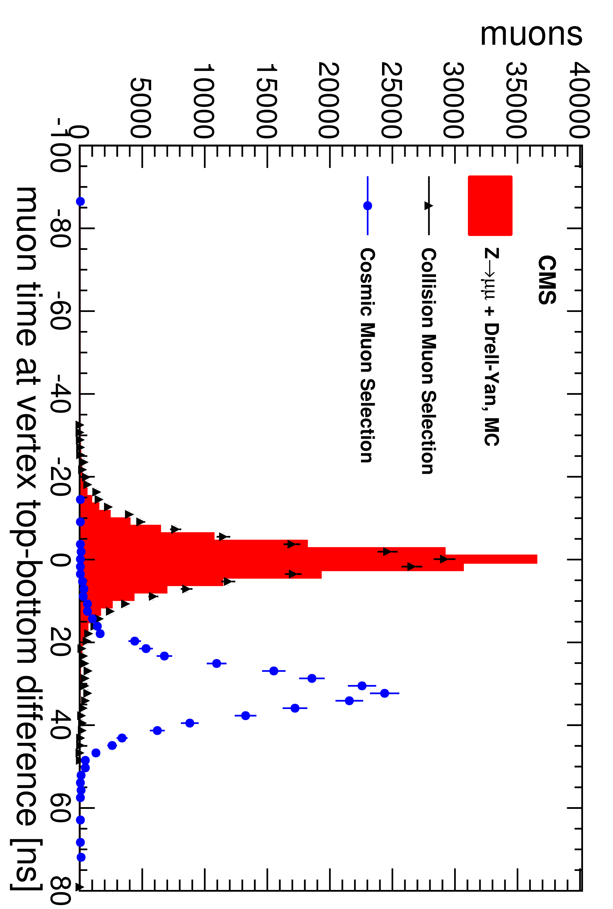
Distributions of variables used for identification of cosmic-ray muons, shown for collision and cosmic-ray muon data samples described in the text, and for ${\mathrm{ Z } } $+Drell-Yan MC samples: (a) muon transverse impact parameter with respect to the nominal beam-spot position; (b) $\log_{10}(\pi -\alpha )$ (see text); (c) muon timing; (d) timing difference between upper and lower muon legs. |
png pdf |
Figure 25-a:
Distributions of variables used for identification of cosmic-ray muons, shown for collision and cosmic-ray muon data samples described in the text, and for ${\mathrm{ Z } } $+Drell-Yan MC samples: (a) muon transverse impact parameter with respect to the nominal beam-spot position; (b) $\log_{10}(\pi -\alpha )$ (see text); (c) muon timing; (d) timing difference between upper and lower muon legs. |
png pdf |
Figure 25-b:
Distributions of variables used for identification of cosmic-ray muons, shown for collision and cosmic-ray muon data samples described in the text, and for ${\mathrm{ Z } } $+Drell-Yan MC samples: (a) muon transverse impact parameter with respect to the nominal beam-spot position; (b) $\log_{10}(\pi -\alpha )$ (see text); (c) muon timing; (d) timing difference between upper and lower muon legs. |
png pdf |
Figure 25-c:
Distributions of variables used for identification of cosmic-ray muons, shown for collision and cosmic-ray muon data samples described in the text, and for ${\mathrm{ Z } } $+Drell-Yan MC samples: (a) muon transverse impact parameter with respect to the nominal beam-spot position; (b) $\log_{10}(\pi -\alpha )$ (see text); (c) muon timing; (d) timing difference between upper and lower muon legs. |
png pdf |
Figure 25-d:
Distributions of variables used for identification of cosmic-ray muons, shown for collision and cosmic-ray muon data samples described in the text, and for ${\mathrm{ Z } } $+Drell-Yan MC samples: (a) muon transverse impact parameter with respect to the nominal beam-spot position; (b) $\log_{10}(\pi -\alpha )$ (see text); (c) muon timing; (d) timing difference between upper and lower muon legs. |

png pdf |
Figure 26:
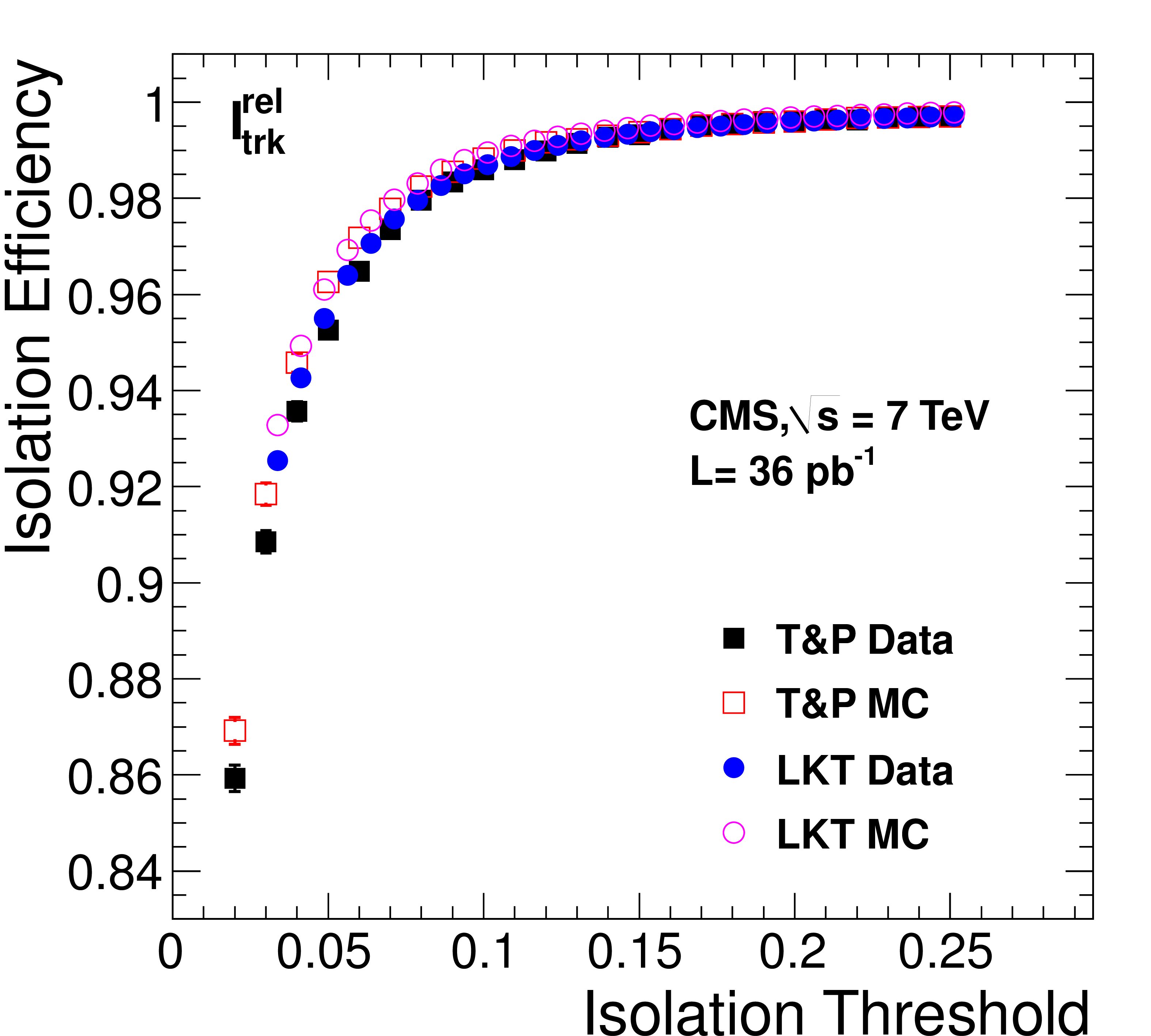
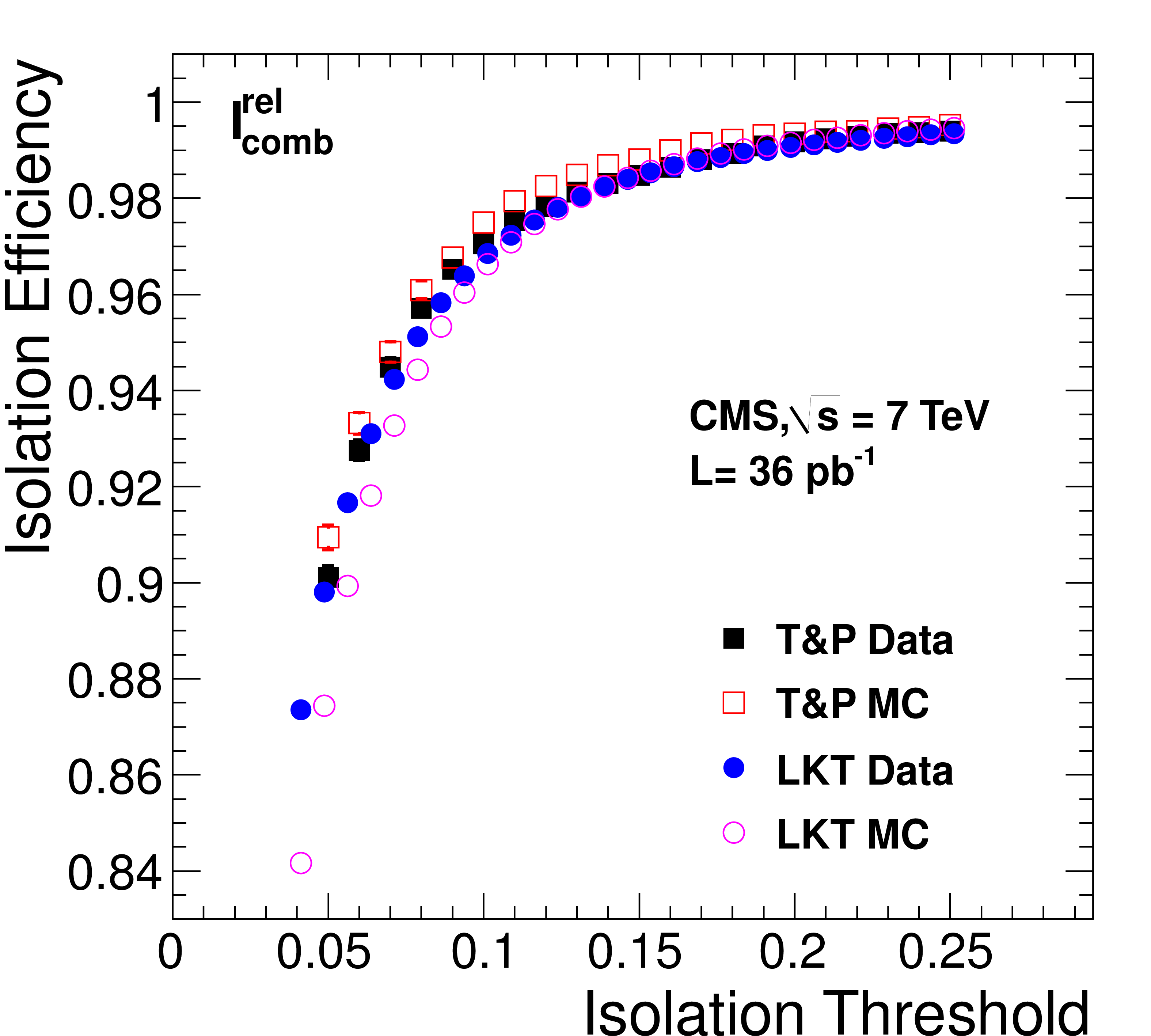
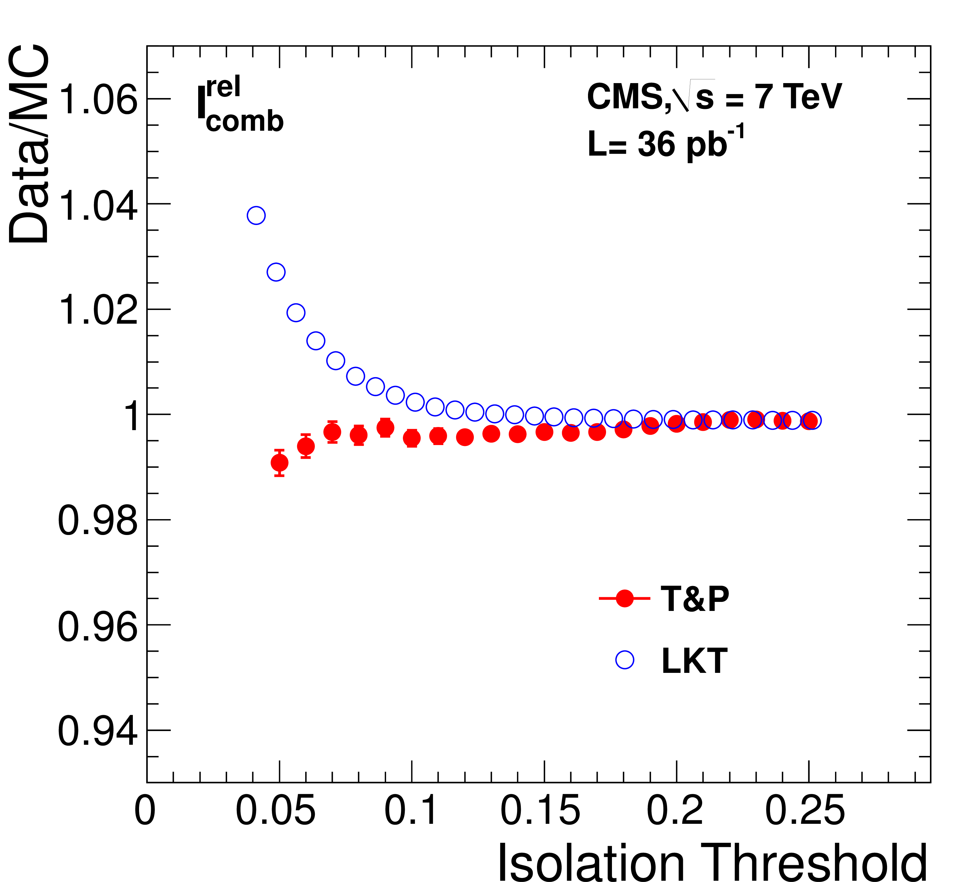
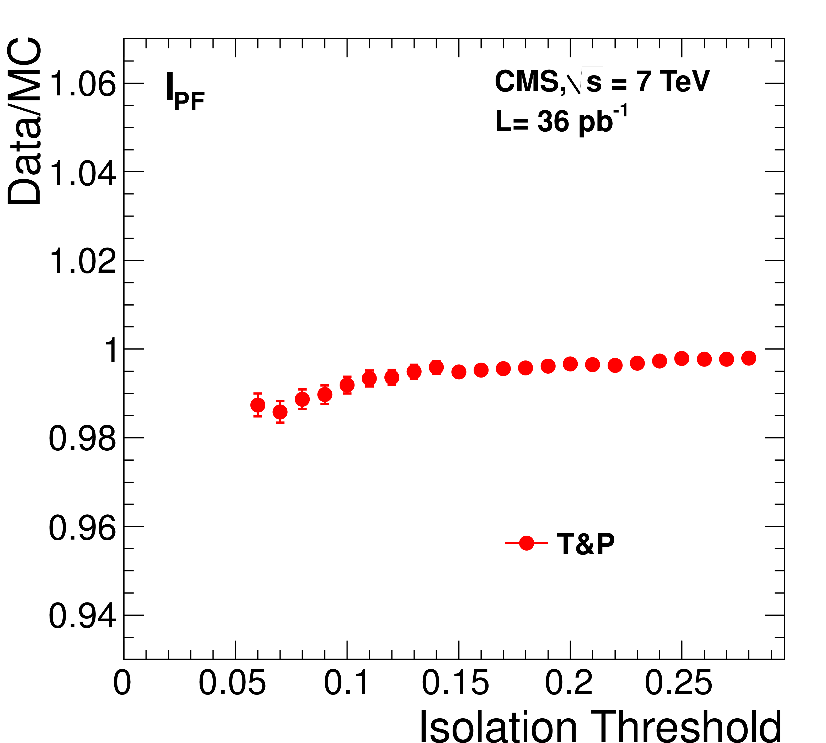
Left: efficiencies of various isolation algorithms for muons with 20 $ < {p_{\mathrm {T}}} < $ 50 GeV/$c$ from ${\mathrm{ Z } } $ decays as a function of the isolation threshold. Results are shown for both data and simulation using the tag-and-probe (``T&P'') and Lepton Kinematic Template (``LKT'') methods; the LKT method is not used for the particle-flow algorithm. Right: data to simulation ratios. Plots are shown for tracker relative ($I^{\text {rel}}_{\text {trk}}$, top), tracker-plus-calorimeters relative ($I^{\text {rel}}_{\text {comb}}$, middle), and particle-flow relative ($I^{\text {rel}}_{\textrm {PF}}$, bottom) isolation algorithms. The MC samples include simulation of pile-up events. |
png pdf |
Figure 26-a:
Left: efficiencies of various isolation algorithms for muons with 20 $ < {p_{\mathrm {T}}} < $ 50 GeV/$c$ from ${\mathrm{ Z } } $ decays as a function of the isolation threshold. Results are shown for both data and simulation using the tag-and-probe (``T&P'') and Lepton Kinematic Template (``LKT'') methods; the LKT method is not used for the particle-flow algorithm. Right: data to simulation ratios. Plots are shown for tracker relative ($I^{\text {rel}}_{\text {trk}}$, top), tracker-plus-calorimeters relative ($I^{\text {rel}}_{\text {comb}}$, middle), and particle-flow relative ($I^{\text {rel}}_{\textrm {PF}}$, bottom) isolation algorithms. The MC samples include simulation of pile-up events. |

png pdf |
Figure 26-b:
Left: efficiencies of various isolation algorithms for muons with 20 $ < {p_{\mathrm {T}}} < $ 50 GeV/$c$ from ${\mathrm{ Z } } $ decays as a function of the isolation threshold. Results are shown for both data and simulation using the tag-and-probe (``T&P'') and Lepton Kinematic Template (``LKT'') methods; the LKT method is not used for the particle-flow algorithm. Right: data to simulation ratios. Plots are shown for tracker relative ($I^{\text {rel}}_{\text {trk}}$, top), tracker-plus-calorimeters relative ($I^{\text {rel}}_{\text {comb}}$, middle), and particle-flow relative ($I^{\text {rel}}_{\textrm {PF}}$, bottom) isolation algorithms. The MC samples include simulation of pile-up events. |
png pdf |
Figure 26-c:
Left: efficiencies of various isolation algorithms for muons with 20 $ < {p_{\mathrm {T}}} < $ 50 GeV/$c$ from ${\mathrm{ Z } } $ decays as a function of the isolation threshold. Results are shown for both data and simulation using the tag-and-probe (``T&P'') and Lepton Kinematic Template (``LKT'') methods; the LKT method is not used for the particle-flow algorithm. Right: data to simulation ratios. Plots are shown for tracker relative ($I^{\text {rel}}_{\text {trk}}$, top), tracker-plus-calorimeters relative ($I^{\text {rel}}_{\text {comb}}$, middle), and particle-flow relative ($I^{\text {rel}}_{\textrm {PF}}$, bottom) isolation algorithms. The MC samples include simulation of pile-up events. |
png pdf |
Figure 26-d:
Left: efficiencies of various isolation algorithms for muons with 20 $ < {p_{\mathrm {T}}} < $ 50 GeV/$c$ from ${\mathrm{ Z } } $ decays as a function of the isolation threshold. Results are shown for both data and simulation using the tag-and-probe (``T&P'') and Lepton Kinematic Template (``LKT'') methods; the LKT method is not used for the particle-flow algorithm. Right: data to simulation ratios. Plots are shown for tracker relative ($I^{\text {rel}}_{\text {trk}}$, top), tracker-plus-calorimeters relative ($I^{\text {rel}}_{\text {comb}}$, middle), and particle-flow relative ($I^{\text {rel}}_{\textrm {PF}}$, bottom) isolation algorithms. The MC samples include simulation of pile-up events. |

png pdf |
Figure 26-e:
Left: efficiencies of various isolation algorithms for muons with 20 $ < {p_{\mathrm {T}}} < $ 50 GeV/$c$ from ${\mathrm{ Z } } $ decays as a function of the isolation threshold. Results are shown for both data and simulation using the tag-and-probe (``T&P'') and Lepton Kinematic Template (``LKT'') methods; the LKT method is not used for the particle-flow algorithm. Right: data to simulation ratios. Plots are shown for tracker relative ($I^{\text {rel}}_{\text {trk}}$, top), tracker-plus-calorimeters relative ($I^{\text {rel}}_{\text {comb}}$, middle), and particle-flow relative ($I^{\text {rel}}_{\textrm {PF}}$, bottom) isolation algorithms. The MC samples include simulation of pile-up events. |
png pdf |
Figure 26-f:
Left: efficiencies of various isolation algorithms for muons with 20 $ < {p_{\mathrm {T}}} < $ 50 GeV/$c$ from ${\mathrm{ Z } } $ decays as a function of the isolation threshold. Results are shown for both data and simulation using the tag-and-probe (``T&P'') and Lepton Kinematic Template (``LKT'') methods; the LKT method is not used for the particle-flow algorithm. Right: data to simulation ratios. Plots are shown for tracker relative ($I^{\text {rel}}_{\text {trk}}$, top), tracker-plus-calorimeters relative ($I^{\text {rel}}_{\text {comb}}$, middle), and particle-flow relative ($I^{\text {rel}}_{\textrm {PF}}$, bottom) isolation algorithms. The MC samples include simulation of pile-up events. |
png pdf |
Figure 27:
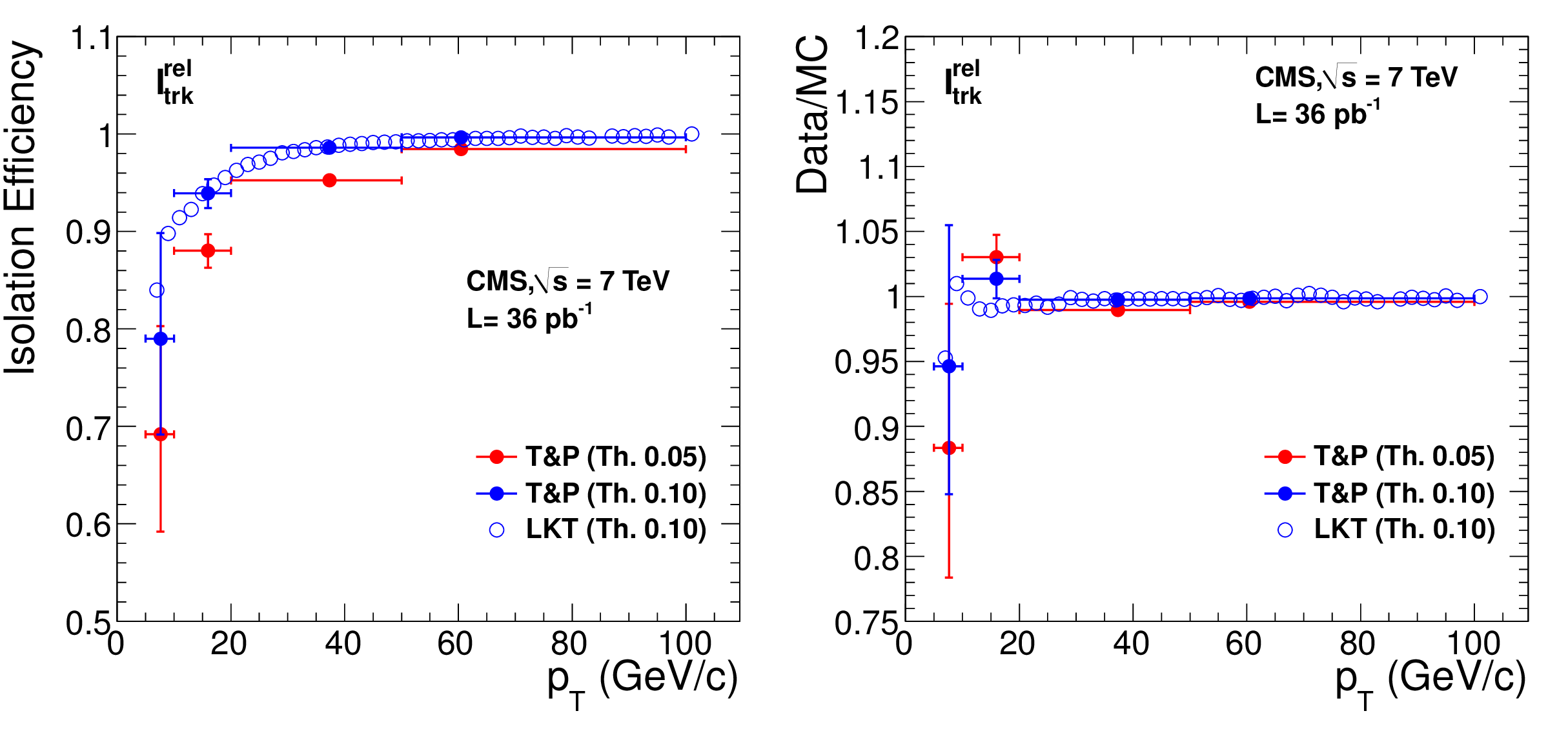
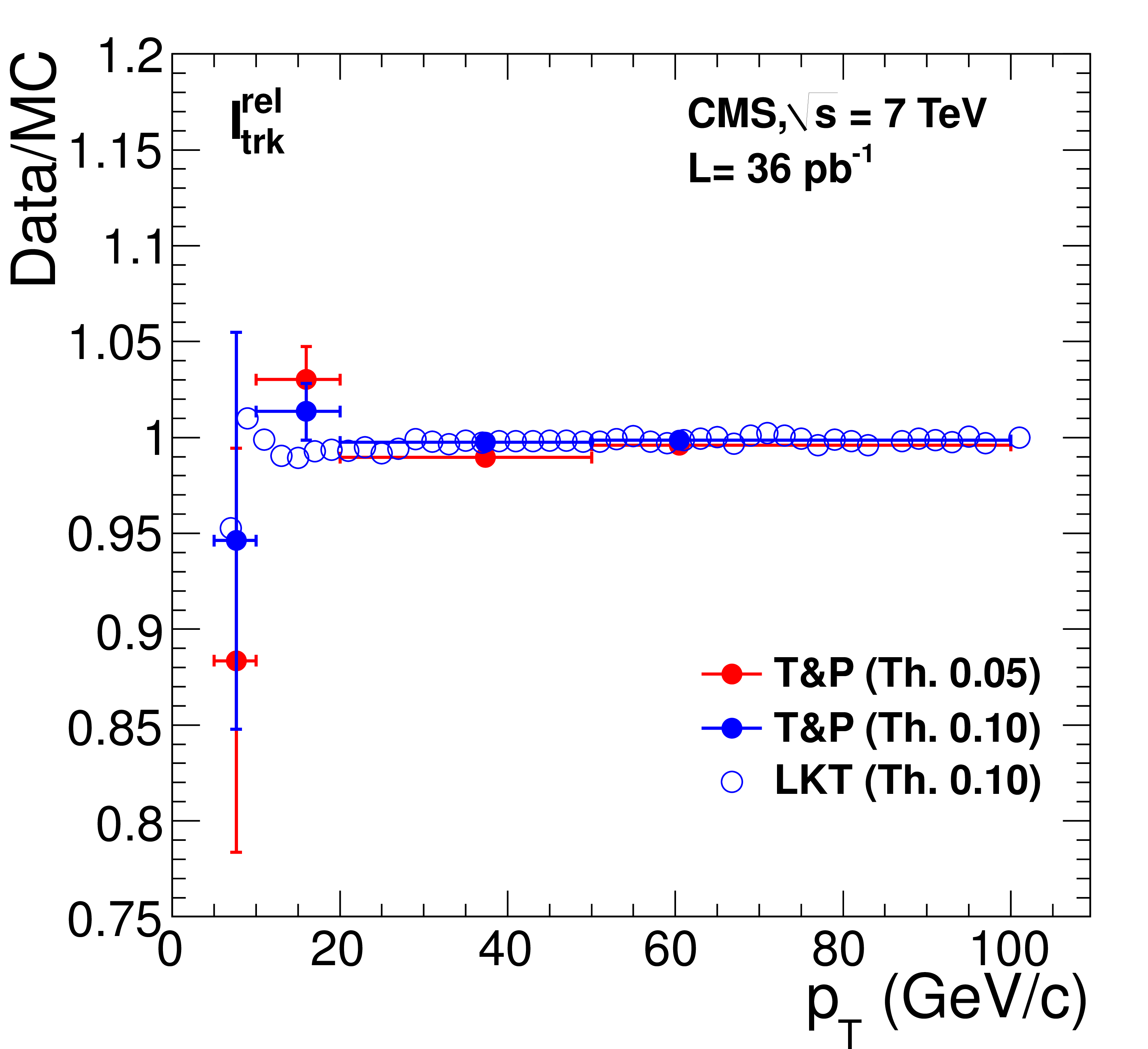
Left: efficiency of tracker relative isolation $I^{\text {rel}}_{\text {trk}}$ for muons from ${\mathrm{ Z } } $ decays as a function of muon $ {p_{\mathrm {T}}} $, measured with data using the tag-and-probe (``T&P'') method (in bins of [5, 10], [10, 20], [20, 50], and [50, 100] GeV/$c$) and the LKT method (finer binning). Results corresponding to the threshold values of 0.05 and 0.1 are shown. Right: ratio between data and MC efficiencies. The MC samples include simulation of pile-up events. |

png pdf |
Figure 27-a:
Left: efficiency of tracker relative isolation $I^{\text {rel}}_{\text {trk}}$ for muons from ${\mathrm{ Z } } $ decays as a function of muon $ {p_{\mathrm {T}}} $, measured with data using the tag-and-probe (``T&P'') method (in bins of [5, 10], [10, 20], [20, 50], and [50, 100] GeV/$c$) and the LKT method (finer binning). Results corresponding to the threshold values of 0.05 and 0.1 are shown. Right: ratio between data and MC efficiencies. The MC samples include simulation of pile-up events. |
png pdf |
Figure 27-b:
Left: efficiency of tracker relative isolation $I^{\text {rel}}_{\text {trk}}$ for muons from ${\mathrm{ Z } } $ decays as a function of muon $ {p_{\mathrm {T}}} $, measured with data using the tag-and-probe (``T&P'') method (in bins of [5, 10], [10, 20], [20, 50], and [50, 100] GeV/$c$) and the LKT method (finer binning). Results corresponding to the threshold values of 0.05 and 0.1 are shown. Right: ratio between data and MC efficiencies. The MC samples include simulation of pile-up events. |
png pdf |
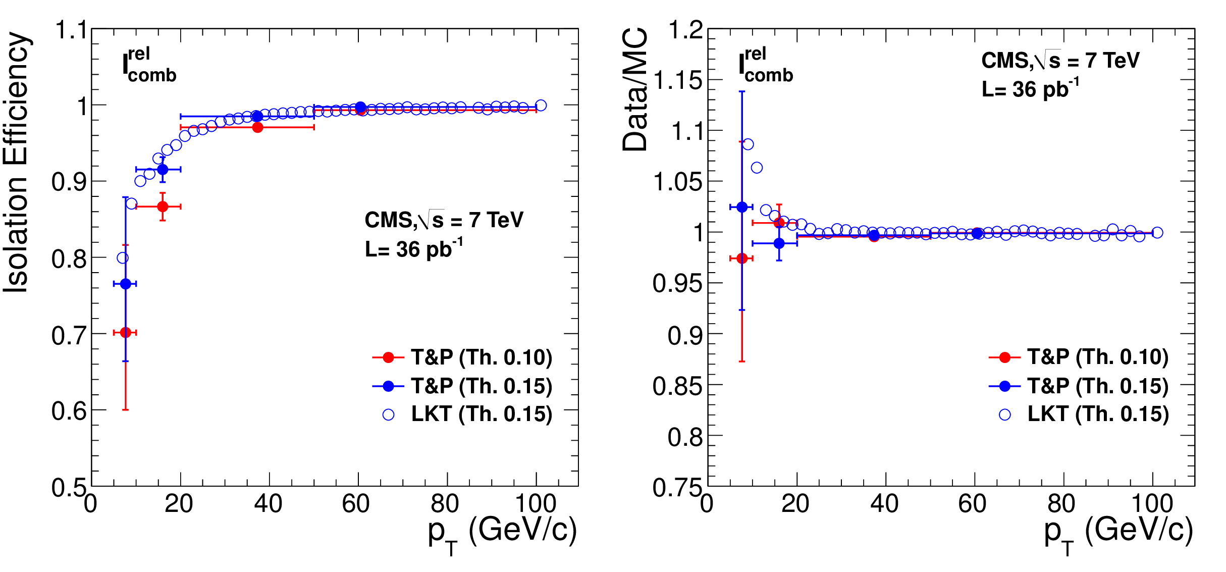
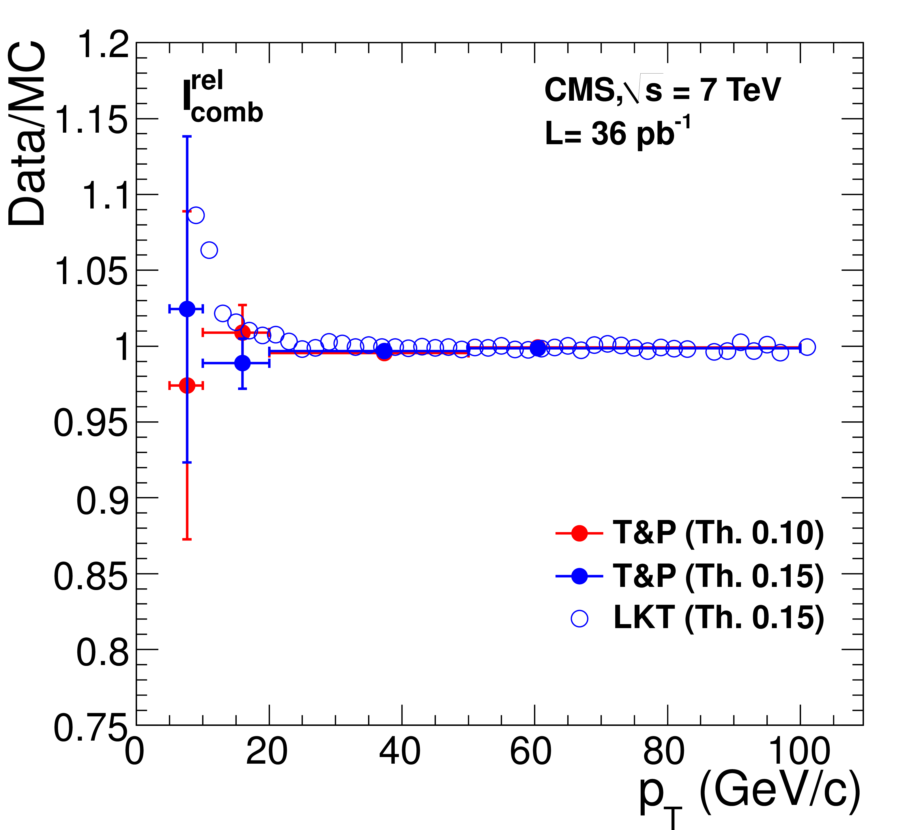
Figure 28:
Left: efficiency of tracker-plus-calorimeters relative isolation $I^{\text {rel}}_{\text {comb}}$ for muons from ${\mathrm{ Z } } $ decays as a function of muon $ {p_{\mathrm {T}}} $, measured with data using the tag-and-probe (``T&P'') method (in bins of [5, 10], [10, 20], [20, 50], and [50, 100] GeV/$c$) and the LKT method (finer binning). Results corresponding to the threshold values of 0.10 and 0.15 are shown. Right: ratio between data and MC efficiencies. The MC samples include simulation of pile-up events. |

png pdf |
Figure 28-a:
Left: efficiency of tracker-plus-calorimeters relative isolation $I^{\text {rel}}_{\text {comb}}$ for muons from ${\mathrm{ Z } } $ decays as a function of muon $ {p_{\mathrm {T}}} $, measured with data using the tag-and-probe (``T&P'') method (in bins of [5, 10], [10, 20], [20, 50], and [50, 100] GeV/$c$) and the LKT method (finer binning). Results corresponding to the threshold values of 0.10 and 0.15 are shown. Right: ratio between data and MC efficiencies. The MC samples include simulation of pile-up events. |
png pdf |
Figure 28-b:
Left: efficiency of tracker-plus-calorimeters relative isolation $I^{\text {rel}}_{\text {comb}}$ for muons from ${\mathrm{ Z } } $ decays as a function of muon $ {p_{\mathrm {T}}} $, measured with data using the tag-and-probe (``T&P'') method (in bins of [5, 10], [10, 20], [20, 50], and [50, 100] GeV/$c$) and the LKT method (finer binning). Results corresponding to the threshold values of 0.10 and 0.15 are shown. Right: ratio between data and MC efficiencies. The MC samples include simulation of pile-up events. |

png pdf |
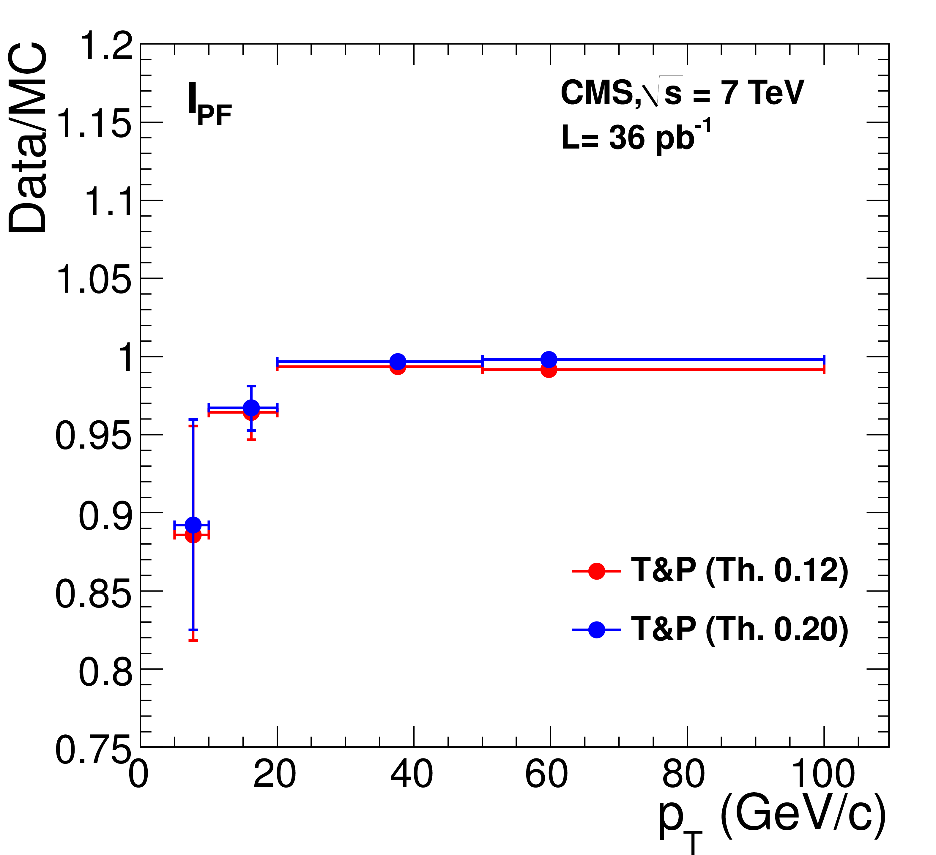
Figure 29:
Left: efficiency of particle-flow relative isolation $I^{\text {rel}}_{\textrm {PF}}$ for muons from ${\mathrm{ Z } } $ decays as a function of muon $ {p_{\mathrm {T}}} $, measured with data using the tag-and-probe (``T&P'') method. Results corresponding to the threshold values of 0.12 and 0.20 are shown. Right: ratio between data and MC efficiencies. The MC samples include simulation of pile-up events. |

png pdf |
Figure 29-a:
Left: efficiency of particle-flow relative isolation $I^{\text {rel}}_{\textrm {PF}}$ for muons from ${\mathrm{ Z } } $ decays as a function of muon $ {p_{\mathrm {T}}} $, measured with data using the tag-and-probe (``T&P'') method. Results corresponding to the threshold values of 0.12 and 0.20 are shown. Right: ratio between data and MC efficiencies. The MC samples include simulation of pile-up events. |
png pdf |
Figure 29-b:
Left: efficiency of particle-flow relative isolation $I^{\text {rel}}_{\textrm {PF}}$ for muons from ${\mathrm{ Z } } $ decays as a function of muon $ {p_{\mathrm {T}}} $, measured with data using the tag-and-probe (``T&P'') method. Results corresponding to the threshold values of 0.12 and 0.20 are shown. Right: ratio between data and MC efficiencies. The MC samples include simulation of pile-up events. |
png pdf |
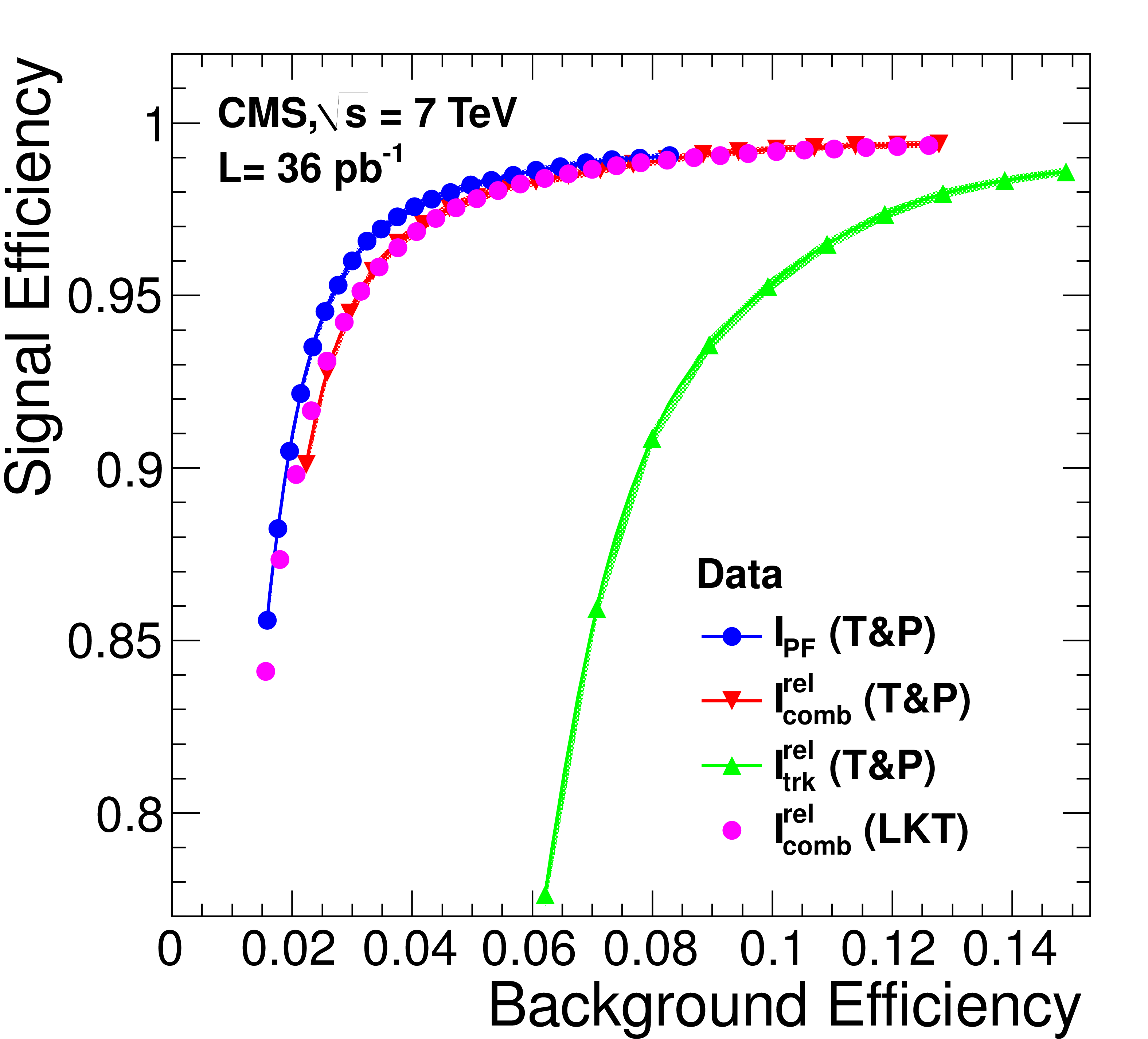
Figure 30:
Isolation efficiency for muons from ${\mathrm{ Z } } $ decays versus isolation efficiency for muons in the QCD-enhanced dataset described in the text, for tracker relative, tracker-plus-calorimeters relative, and particle-flow relative isolation algorithms. Muons are required to have $ {p_{\mathrm {T}}} $ in the range between 20 and 50 GeV/$c$. The background rejection is limited by the 0.4% contamination from truly isolated muons. |
png pdf |
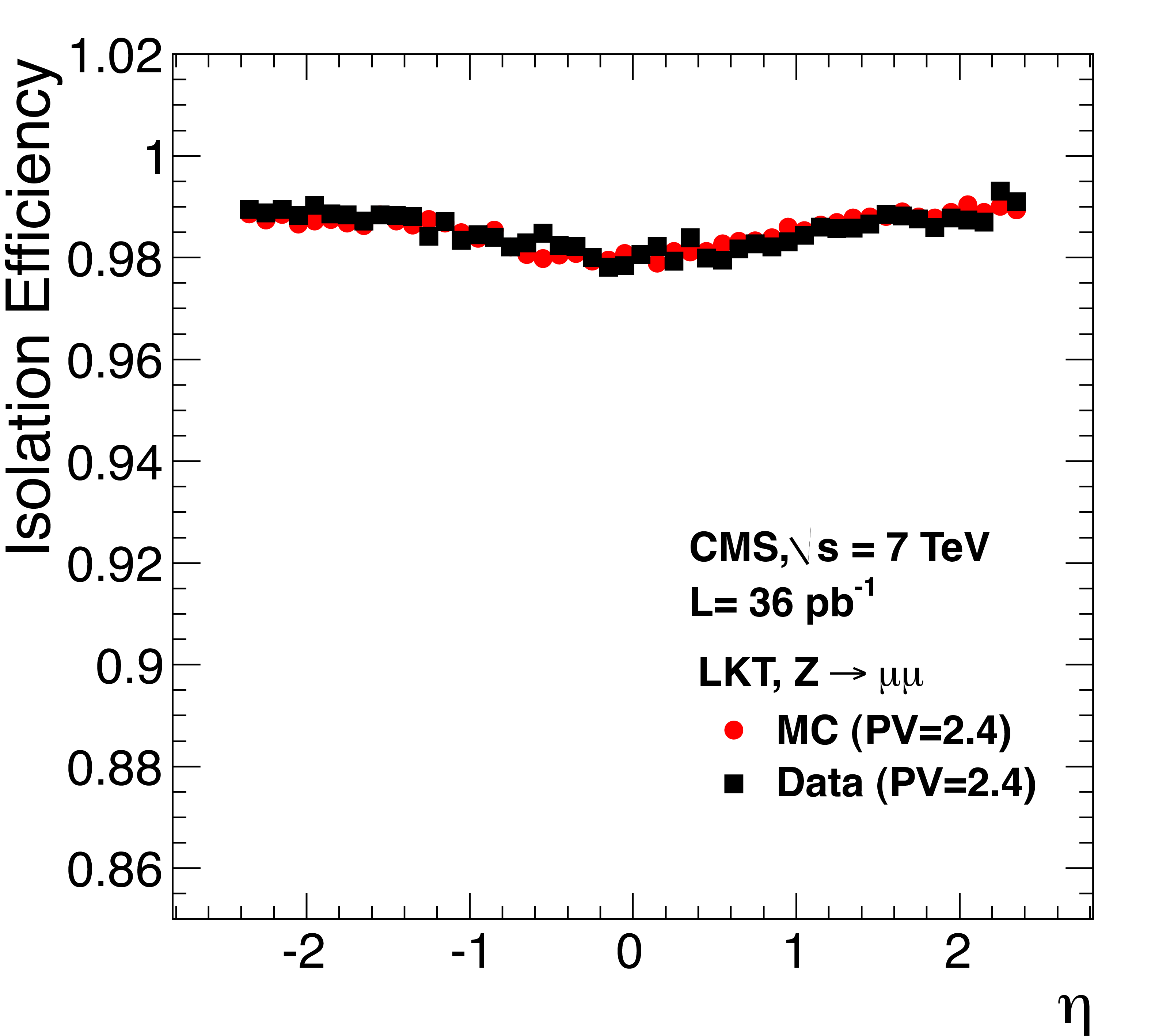
Figure 31:
Muon isolation efficiency versus $\eta $. Efficiency for muons with $ {p_{\mathrm {T}}} $ between 20 and 50 GeV/$c$ from ${\mathrm{ Z } } $ decays observed in 2010 data, in which the average number of reconstructed primary vertices (PV) is 2.4, is compared with the results obtained using MC samples with the same average number of primary vertices. The results were obtained with the LKT method using the $I^{\text {rel}}_{\text {comb}}$ algorithm with a threshold of 0.15. |
png pdf |
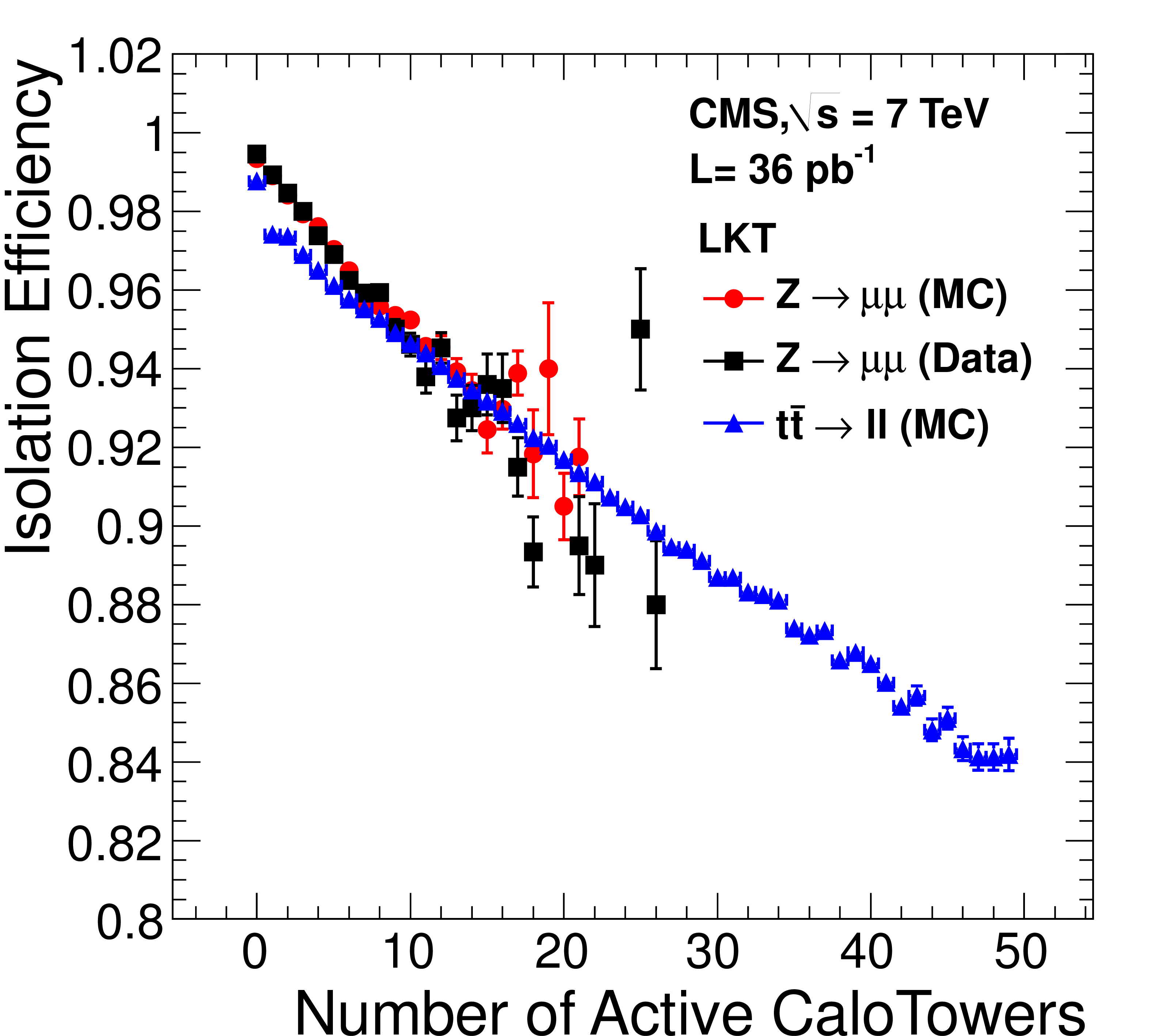
Figure 32:
Muon isolation efficiency versus number of calorimeter towers in the region of $|\eta | < 2.7$ having transverse energy larger than 1 GeV. Results for muons with $20< {p_{\mathrm {T}}} < $ 50 GeV/$c$ from ${\mathrm{ Z } } $ decays obtained in data and in simulation are compared with the efficiency for prompt muons in a simulated sample of top pairs decaying leptonically. All results were obtained with the LKT method using the $I^{\text {rel}}_{\text {comb}}$ algorithm with a threshold of 0.15. The MC samples include simulation of pile-up events. |
png pdf |
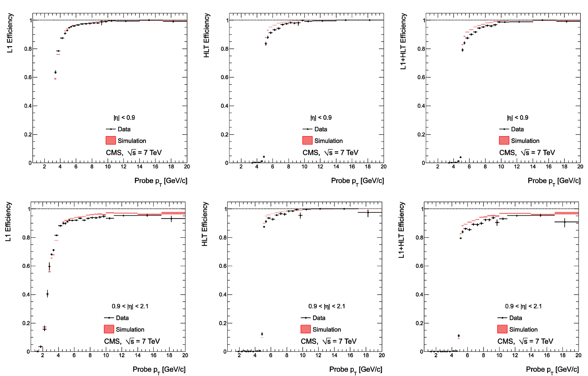
Figure 33:
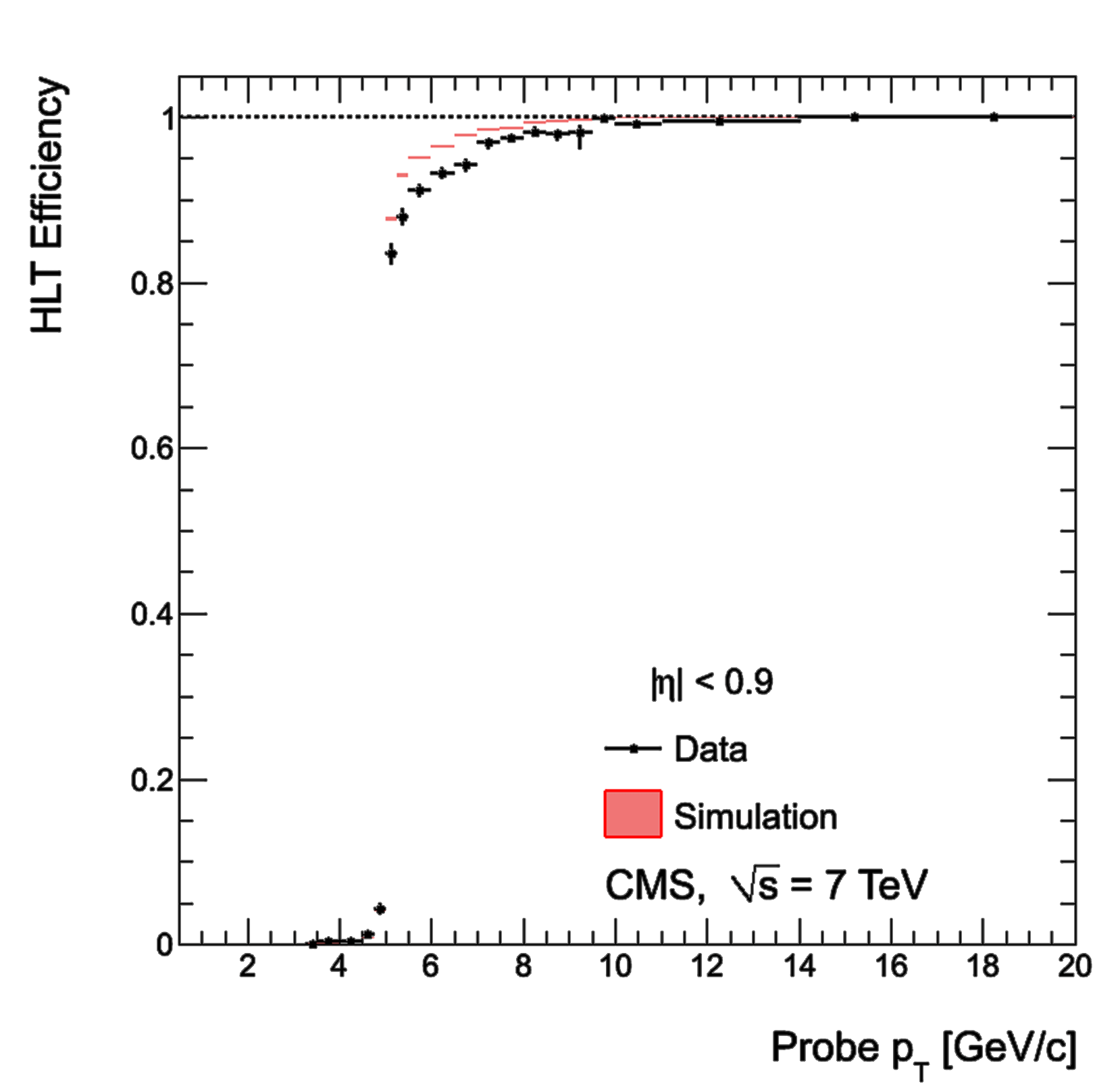
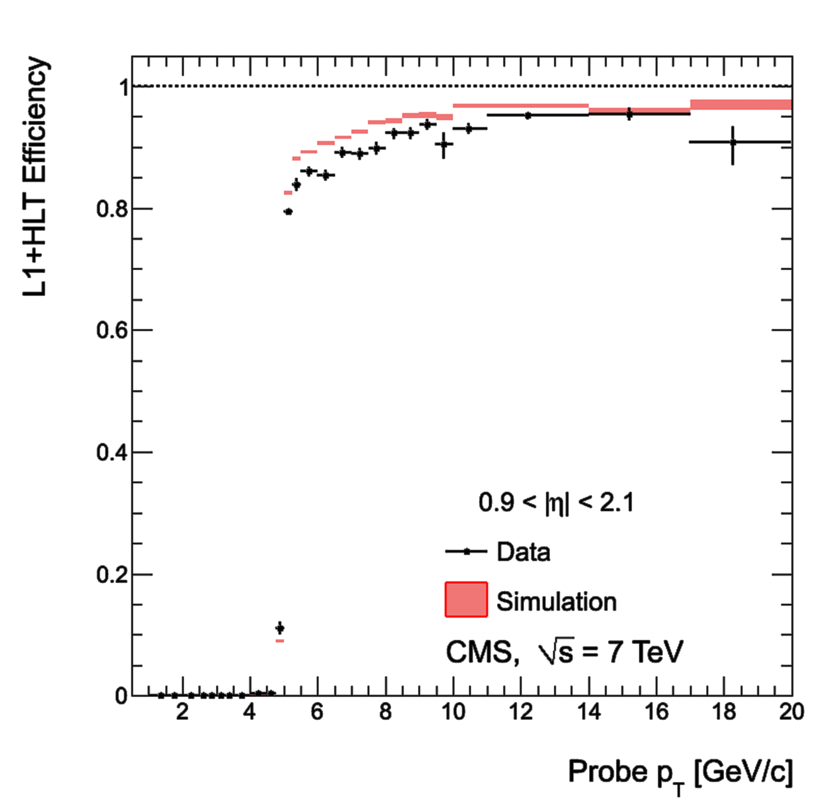
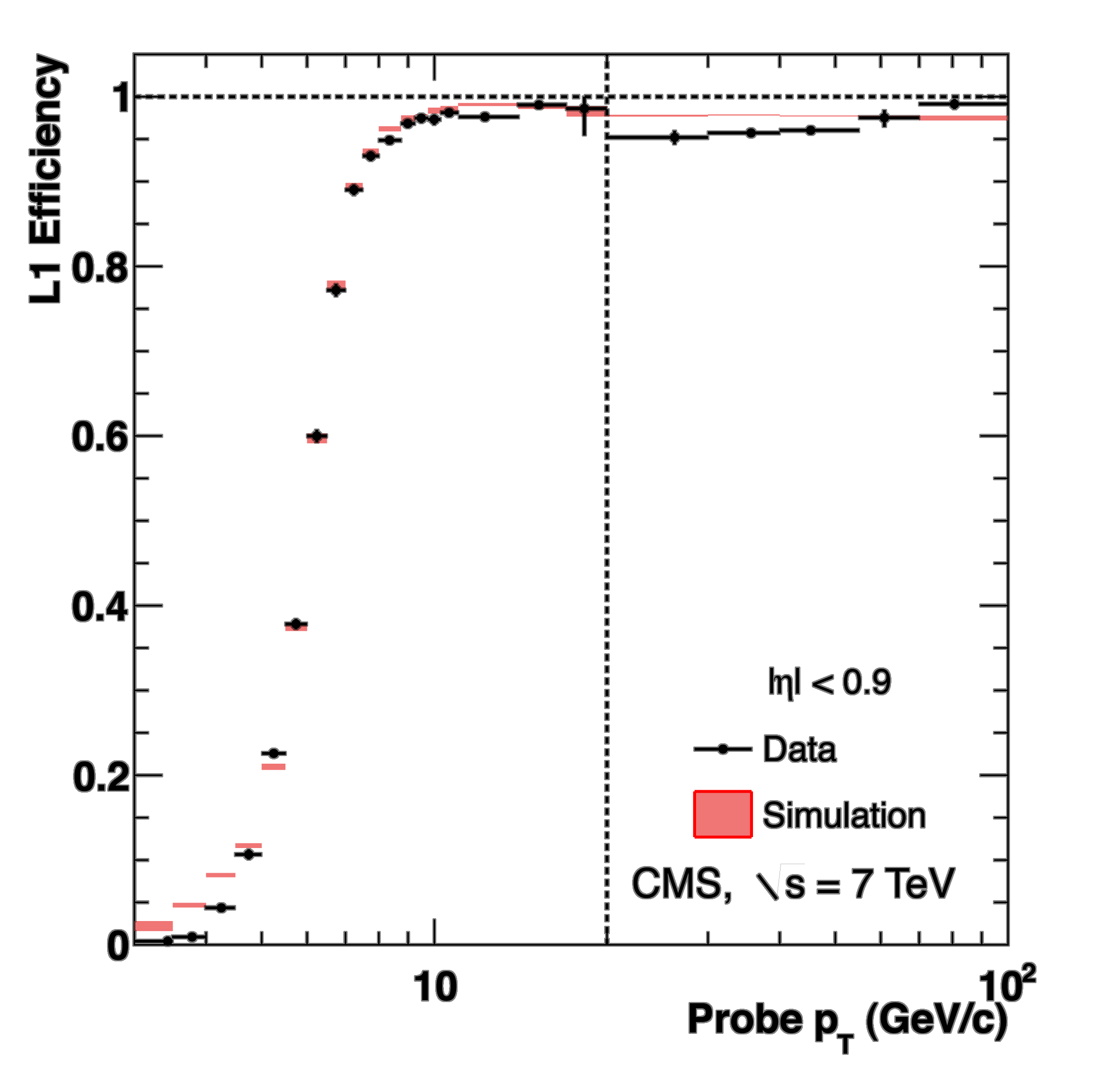
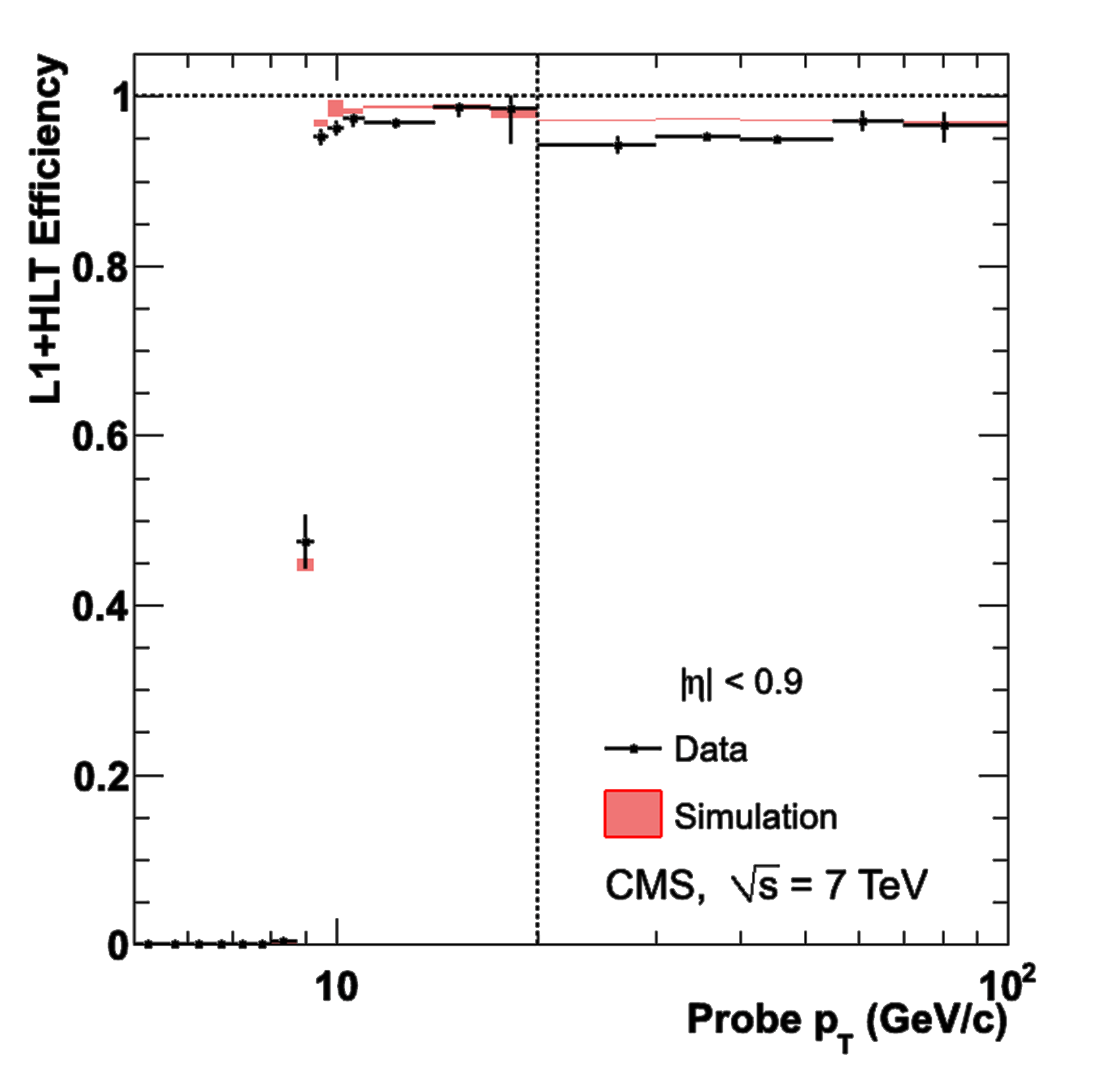
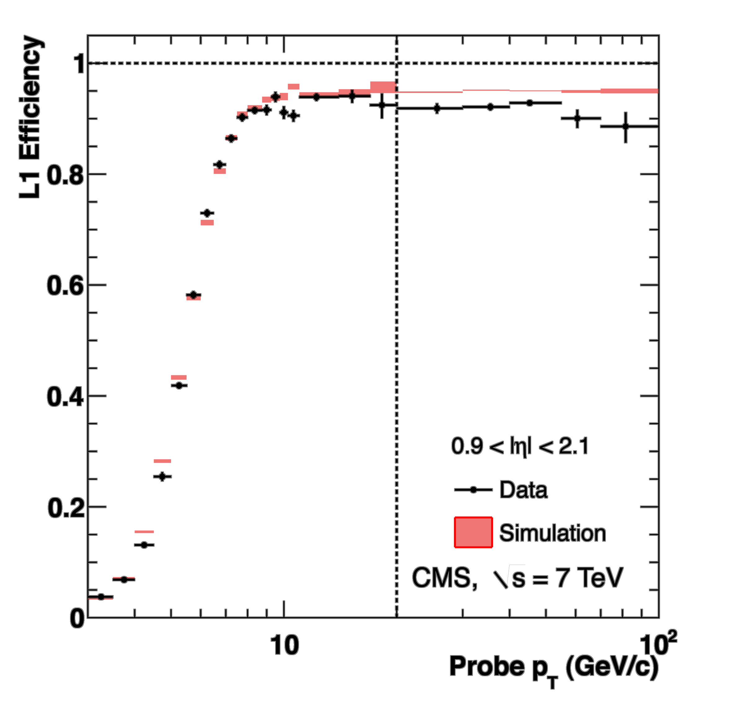
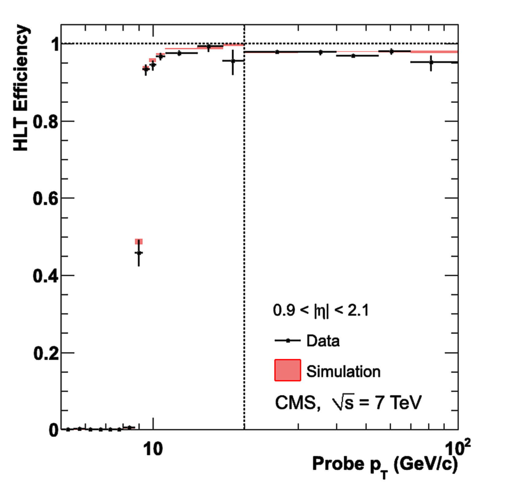
Single-muon trigger efficiencies for Soft Muons as a function of the Soft Muon $ {p_{\mathrm {T}}} $ in the barrel (top) and the overlap-endcap (bottom) regions: the efficiency of the Level-1 trigger with $ {p_{\mathrm {T}}} $ threshold at 3 GeV/$c$ (left), the efficiency of the HLT with $ {p_{\mathrm {T}}} $ threshold of 5 GeV/$c$ with respect to Level-1 (middle), and the combined efficiency of Level-1 and HLT (right). The efficiencies obtained using $\mathrm {J}/\psi \to \mu ^+\mu ^-$ events (points with error bars) are compared with predictions from the MC simulation ($\pm$1$\sigma$ bands); the uncertainties are statistical only. |

png |
Figure 33-a:
Single-muon trigger efficiencies for Soft Muons as a function of the Soft Muon $ {p_{\mathrm {T}}} $ in the barrel (top) and the overlap-endcap (bottom) regions: the efficiency of the Level-1 trigger with $ {p_{\mathrm {T}}} $ threshold at 3 GeV/$c$ (left), the efficiency of the HLT with $ {p_{\mathrm {T}}} $ threshold of 5 GeV/$c$ with respect to Level-1 (middle), and the combined efficiency of Level-1 and HLT (right). The efficiencies obtained using $\mathrm {J}/\psi \to \mu ^+\mu ^-$ events (points with error bars) are compared with predictions from the MC simulation ($\pm$1$\sigma$ bands); the uncertainties are statistical only. |
png |
Figure 33-b:
Single-muon trigger efficiencies for Soft Muons as a function of the Soft Muon $ {p_{\mathrm {T}}} $ in the barrel (top) and the overlap-endcap (bottom) regions: the efficiency of the Level-1 trigger with $ {p_{\mathrm {T}}} $ threshold at 3 GeV/$c$ (left), the efficiency of the HLT with $ {p_{\mathrm {T}}} $ threshold of 5 GeV/$c$ with respect to Level-1 (middle), and the combined efficiency of Level-1 and HLT (right). The efficiencies obtained using $\mathrm {J}/\psi \to \mu ^+\mu ^-$ events (points with error bars) are compared with predictions from the MC simulation ($\pm$1$\sigma$ bands); the uncertainties are statistical only. |

png |
Figure 33-c:
Single-muon trigger efficiencies for Soft Muons as a function of the Soft Muon $ {p_{\mathrm {T}}} $ in the barrel (top) and the overlap-endcap (bottom) regions: the efficiency of the Level-1 trigger with $ {p_{\mathrm {T}}} $ threshold at 3 GeV/$c$ (left), the efficiency of the HLT with $ {p_{\mathrm {T}}} $ threshold of 5 GeV/$c$ with respect to Level-1 (middle), and the combined efficiency of Level-1 and HLT (right). The efficiencies obtained using $\mathrm {J}/\psi \to \mu ^+\mu ^-$ events (points with error bars) are compared with predictions from the MC simulation ($\pm$1$\sigma$ bands); the uncertainties are statistical only. |

png |
Figure 33-d:
Single-muon trigger efficiencies for Soft Muons as a function of the Soft Muon $ {p_{\mathrm {T}}} $ in the barrel (top) and the overlap-endcap (bottom) regions: the efficiency of the Level-1 trigger with $ {p_{\mathrm {T}}} $ threshold at 3 GeV/$c$ (left), the efficiency of the HLT with $ {p_{\mathrm {T}}} $ threshold of 5 GeV/$c$ with respect to Level-1 (middle), and the combined efficiency of Level-1 and HLT (right). The efficiencies obtained using $\mathrm {J}/\psi \to \mu ^+\mu ^-$ events (points with error bars) are compared with predictions from the MC simulation ($\pm$1$\sigma$ bands); the uncertainties are statistical only. |

png |
Figure 33-e:
Single-muon trigger efficiencies for Soft Muons as a function of the Soft Muon $ {p_{\mathrm {T}}} $ in the barrel (top) and the overlap-endcap (bottom) regions: the efficiency of the Level-1 trigger with $ {p_{\mathrm {T}}} $ threshold at 3 GeV/$c$ (left), the efficiency of the HLT with $ {p_{\mathrm {T}}} $ threshold of 5 GeV/$c$ with respect to Level-1 (middle), and the combined efficiency of Level-1 and HLT (right). The efficiencies obtained using $\mathrm {J}/\psi \to \mu ^+\mu ^-$ events (points with error bars) are compared with predictions from the MC simulation ($\pm$1$\sigma$ bands); the uncertainties are statistical only. |
png |
Figure 33-f:
Single-muon trigger efficiencies for Soft Muons as a function of the Soft Muon $ {p_{\mathrm {T}}} $ in the barrel (top) and the overlap-endcap (bottom) regions: the efficiency of the Level-1 trigger with $ {p_{\mathrm {T}}} $ threshold at 3 GeV/$c$ (left), the efficiency of the HLT with $ {p_{\mathrm {T}}} $ threshold of 5 GeV/$c$ with respect to Level-1 (middle), and the combined efficiency of Level-1 and HLT (right). The efficiencies obtained using $\mathrm {J}/\psi \to \mu ^+\mu ^-$ events (points with error bars) are compared with predictions from the MC simulation ($\pm$1$\sigma$ bands); the uncertainties are statistical only. |
png pdf |
Figure 34:
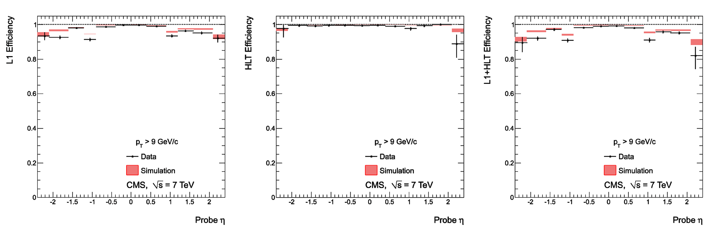
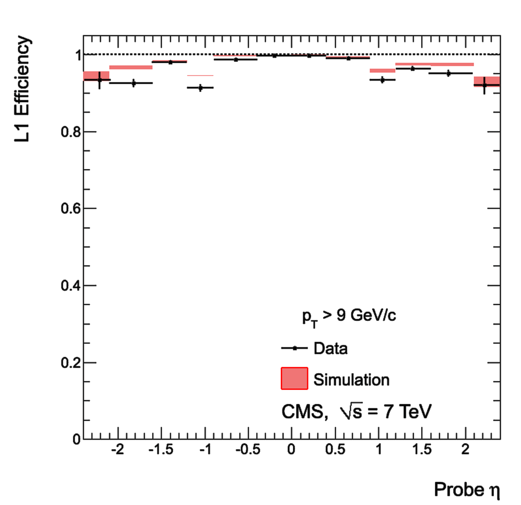
Single-muon trigger efficiencies for Soft Muons as a function of the Soft Muon $\eta $, for muons with $ {p_{\mathrm {T}}} $ in the range of 9 $ < {p_{\mathrm {T}}} < 20 $ GeV/$c$: the efficiency of the Level-1 trigger with $ {p_{\mathrm {T}}} $ threshold at 3 GeV/$c$ (left), the efficiency of the HLT with $ {p_{\mathrm {T}}} $ threshold of 5 GeV/$c$ with respect to Level-1 (middle), and the combined efficiency of Level-1 and HLT (right). The efficiencies obtained using $\mathrm {J}/\psi \to \mu ^+\mu ^-$ events (points with error bars) are compared with predictions from the MC simulation ($\pm$1$\sigma$ bands); the uncertainties are statistical only. |
png |
Figure 34-a:
Single-muon trigger efficiencies for Soft Muons as a function of the Soft Muon $\eta $, for muons with $ {p_{\mathrm {T}}} $ in the range of 9 $ < {p_{\mathrm {T}}} < 20 $ GeV/$c$: the efficiency of the Level-1 trigger with $ {p_{\mathrm {T}}} $ threshold at 3 GeV/$c$ (left), the efficiency of the HLT with $ {p_{\mathrm {T}}} $ threshold of 5 GeV/$c$ with respect to Level-1 (middle), and the combined efficiency of Level-1 and HLT (right). The efficiencies obtained using $\mathrm {J}/\psi \to \mu ^+\mu ^-$ events (points with error bars) are compared with predictions from the MC simulation ($\pm$1$\sigma$ bands); the uncertainties are statistical only. |

png |
Figure 34-b:
Single-muon trigger efficiencies for Soft Muons as a function of the Soft Muon $\eta $, for muons with $ {p_{\mathrm {T}}} $ in the range of 9 $ < {p_{\mathrm {T}}} < 20 $ GeV/$c$: the efficiency of the Level-1 trigger with $ {p_{\mathrm {T}}} $ threshold at 3 GeV/$c$ (left), the efficiency of the HLT with $ {p_{\mathrm {T}}} $ threshold of 5 GeV/$c$ with respect to Level-1 (middle), and the combined efficiency of Level-1 and HLT (right). The efficiencies obtained using $\mathrm {J}/\psi \to \mu ^+\mu ^-$ events (points with error bars) are compared with predictions from the MC simulation ($\pm$1$\sigma$ bands); the uncertainties are statistical only. |

png |
Figure 34-c:
Single-muon trigger efficiencies for Soft Muons as a function of the Soft Muon $\eta $, for muons with $ {p_{\mathrm {T}}} $ in the range of 9 $ < {p_{\mathrm {T}}} < 20 $ GeV/$c$: the efficiency of the Level-1 trigger with $ {p_{\mathrm {T}}} $ threshold at 3 GeV/$c$ (left), the efficiency of the HLT with $ {p_{\mathrm {T}}} $ threshold of 5 GeV/$c$ with respect to Level-1 (middle), and the combined efficiency of Level-1 and HLT (right). The efficiencies obtained using $\mathrm {J}/\psi \to \mu ^+\mu ^-$ events (points with error bars) are compared with predictions from the MC simulation ($\pm$1$\sigma$ bands); the uncertainties are statistical only. |

png pdf |
Figure 35:
Single-muon trigger efficiencies for Tight Muons as a function of the Tight Muon $ {p_{\mathrm {T}}} $ in the barrel (top) and the overlap-endcap (bottom) regions. The measurements are done with the tag-and-probe method, using $\mathrm {J}/\psi \to \mu ^+\mu ^-$ events for $ {p_{\mathrm {T}}} $ below 20 GeV/$c$ and $ {\mathrm {Z}}\to \mu ^+\mu ^-$ events above. The efficiencies are shown for the following triggers: Level-1 with $ {p_{\mathrm {T}}} > $ 7 GeV/$c$ threshold (left), HLT with $ {p_{\mathrm {T}}} $ threshold at 9 GeV/$c$ for $ {p_{\mathrm {T}}} $ below 20 GeV/$c$ and at 15 GeV/$c$ above (centre), and the combination of the above Level-1 and HLT triggers (right). The efficiencies in data (points with error bars) are compared with predictions from the simulation ($\pm$1$\sigma$ bands); the uncertainties are statistical only. |
png |
Figure 35-a:
Single-muon trigger efficiencies for Tight Muons as a function of the Tight Muon $ {p_{\mathrm {T}}} $ in the barrel (top) and the overlap-endcap (bottom) regions. The measurements are done with the tag-and-probe method, using $\mathrm {J}/\psi \to \mu ^+\mu ^-$ events for $ {p_{\mathrm {T}}} $ below 20 GeV/$c$ and $ {\mathrm {Z}}\to \mu ^+\mu ^-$ events above. The efficiencies are shown for the following triggers: Level-1 with $ {p_{\mathrm {T}}} > $ 7 GeV/$c$ threshold (left), HLT with $ {p_{\mathrm {T}}} $ threshold at 9 GeV/$c$ for $ {p_{\mathrm {T}}} $ below 20 GeV/$c$ and at 15 GeV/$c$ above (centre), and the combination of the above Level-1 and HLT triggers (right). The efficiencies in data (points with error bars) are compared with predictions from the simulation ($\pm$1$\sigma$ bands); the uncertainties are statistical only. |

png |
Figure 35-b:
Single-muon trigger efficiencies for Tight Muons as a function of the Tight Muon $ {p_{\mathrm {T}}} $ in the barrel (top) and the overlap-endcap (bottom) regions. The measurements are done with the tag-and-probe method, using $\mathrm {J}/\psi \to \mu ^+\mu ^-$ events for $ {p_{\mathrm {T}}} $ below 20 GeV/$c$ and $ {\mathrm {Z}}\to \mu ^+\mu ^-$ events above. The efficiencies are shown for the following triggers: Level-1 with $ {p_{\mathrm {T}}} > $ 7 GeV/$c$ threshold (left), HLT with $ {p_{\mathrm {T}}} $ threshold at 9 GeV/$c$ for $ {p_{\mathrm {T}}} $ below 20 GeV/$c$ and at 15 GeV/$c$ above (centre), and the combination of the above Level-1 and HLT triggers (right). The efficiencies in data (points with error bars) are compared with predictions from the simulation ($\pm$1$\sigma$ bands); the uncertainties are statistical only. |
png |
Figure 35-c:
Single-muon trigger efficiencies for Tight Muons as a function of the Tight Muon $ {p_{\mathrm {T}}} $ in the barrel (top) and the overlap-endcap (bottom) regions. The measurements are done with the tag-and-probe method, using $\mathrm {J}/\psi \to \mu ^+\mu ^-$ events for $ {p_{\mathrm {T}}} $ below 20 GeV/$c$ and $ {\mathrm {Z}}\to \mu ^+\mu ^-$ events above. The efficiencies are shown for the following triggers: Level-1 with $ {p_{\mathrm {T}}} > $ 7 GeV/$c$ threshold (left), HLT with $ {p_{\mathrm {T}}} $ threshold at 9 GeV/$c$ for $ {p_{\mathrm {T}}} $ below 20 GeV/$c$ and at 15 GeV/$c$ above (centre), and the combination of the above Level-1 and HLT triggers (right). The efficiencies in data (points with error bars) are compared with predictions from the simulation ($\pm$1$\sigma$ bands); the uncertainties are statistical only. |
png |
Figure 35-d:
Single-muon trigger efficiencies for Tight Muons as a function of the Tight Muon $ {p_{\mathrm {T}}} $ in the barrel (top) and the overlap-endcap (bottom) regions. The measurements are done with the tag-and-probe method, using $\mathrm {J}/\psi \to \mu ^+\mu ^-$ events for $ {p_{\mathrm {T}}} $ below 20 GeV/$c$ and $ {\mathrm {Z}}\to \mu ^+\mu ^-$ events above. The efficiencies are shown for the following triggers: Level-1 with $ {p_{\mathrm {T}}} > $ 7 GeV/$c$ threshold (left), HLT with $ {p_{\mathrm {T}}} $ threshold at 9 GeV/$c$ for $ {p_{\mathrm {T}}} $ below 20 GeV/$c$ and at 15 GeV/$c$ above (centre), and the combination of the above Level-1 and HLT triggers (right). The efficiencies in data (points with error bars) are compared with predictions from the simulation ($\pm$1$\sigma$ bands); the uncertainties are statistical only. |
png |
Figure 35-e:
Single-muon trigger efficiencies for Tight Muons as a function of the Tight Muon $ {p_{\mathrm {T}}} $ in the barrel (top) and the overlap-endcap (bottom) regions. The measurements are done with the tag-and-probe method, using $\mathrm {J}/\psi \to \mu ^+\mu ^-$ events for $ {p_{\mathrm {T}}} $ below 20 GeV/$c$ and $ {\mathrm {Z}}\to \mu ^+\mu ^-$ events above. The efficiencies are shown for the following triggers: Level-1 with $ {p_{\mathrm {T}}} > $ 7 GeV/$c$ threshold (left), HLT with $ {p_{\mathrm {T}}} $ threshold at 9 GeV/$c$ for $ {p_{\mathrm {T}}} $ below 20 GeV/$c$ and at 15 GeV/$c$ above (centre), and the combination of the above Level-1 and HLT triggers (right). The efficiencies in data (points with error bars) are compared with predictions from the simulation ($\pm$1$\sigma$ bands); the uncertainties are statistical only. |

png |
Figure 35-f:
Single-muon trigger efficiencies for Tight Muons as a function of the Tight Muon $ {p_{\mathrm {T}}} $ in the barrel (top) and the overlap-endcap (bottom) regions. The measurements are done with the tag-and-probe method, using $\mathrm {J}/\psi \to \mu ^+\mu ^-$ events for $ {p_{\mathrm {T}}} $ below 20 GeV/$c$ and $ {\mathrm {Z}}\to \mu ^+\mu ^-$ events above. The efficiencies are shown for the following triggers: Level-1 with $ {p_{\mathrm {T}}} > $ 7 GeV/$c$ threshold (left), HLT with $ {p_{\mathrm {T}}} $ threshold at 9 GeV/$c$ for $ {p_{\mathrm {T}}} $ below 20 GeV/$c$ and at 15 GeV/$c$ above (centre), and the combination of the above Level-1 and HLT triggers (right). The efficiencies in data (points with error bars) are compared with predictions from the simulation ($\pm$1$\sigma$ bands); the uncertainties are statistical only. |
png pdf |
Figure 36:
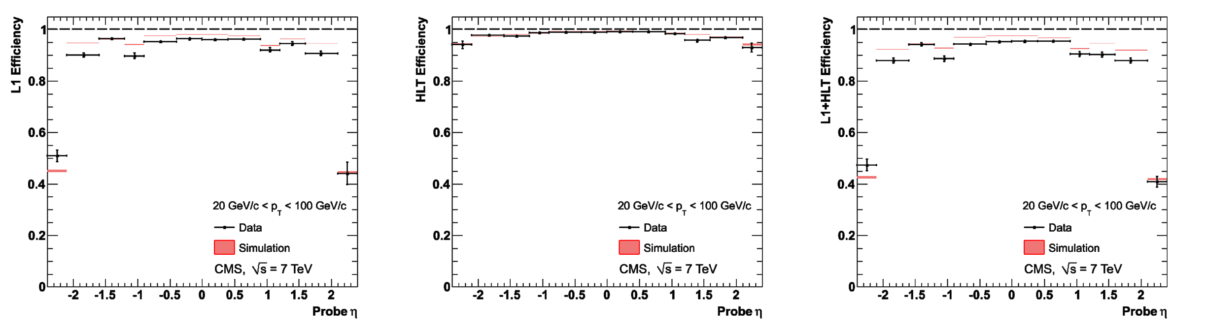
Single-muon trigger efficiencies for Tight Muons with $ {p_{\mathrm {T}}} > $ 20 GeV/$c$ as a function of the Tight Muon $\eta $: the efficiency of the Level-1 trigger with $ {p_{\mathrm {T}}} $ threshold at 7 GeV/$c$ (left), the efficiency of the HLT with $ {p_{\mathrm {T}}} $ threshold of 15 GeV/$c$ with respect to Level-1 (middle), and the combined efficiency of Level-1 and HLT (right). The efficiencies obtained using $ {\mathrm {Z}}\to \mu ^+\mu ^-$ events (points with error bars) are compared with predictions from the MC simulation ($\pm$1$\sigma$ bands); the uncertainties are statistical only. |

png |
Figure 36-a:
Single-muon trigger efficiencies for Tight Muons with $ {p_{\mathrm {T}}} > $ 20 GeV/$c$ as a function of the Tight Muon $\eta $: the efficiency of the Level-1 trigger with $ {p_{\mathrm {T}}} $ threshold at 7 GeV/$c$ (left), the efficiency of the HLT with $ {p_{\mathrm {T}}} $ threshold of 15 GeV/$c$ with respect to Level-1 (middle), and the combined efficiency of Level-1 and HLT (right). The efficiencies obtained using $ {\mathrm {Z}}\to \mu ^+\mu ^-$ events (points with error bars) are compared with predictions from the MC simulation ($\pm$1$\sigma$ bands); the uncertainties are statistical only. |

png |
Figure 36-b:
Single-muon trigger efficiencies for Tight Muons with $ {p_{\mathrm {T}}} > $ 20 GeV/$c$ as a function of the Tight Muon $\eta $: the efficiency of the Level-1 trigger with $ {p_{\mathrm {T}}} $ threshold at 7 GeV/$c$ (left), the efficiency of the HLT with $ {p_{\mathrm {T}}} $ threshold of 15 GeV/$c$ with respect to Level-1 (middle), and the combined efficiency of Level-1 and HLT (right). The efficiencies obtained using $ {\mathrm {Z}}\to \mu ^+\mu ^-$ events (points with error bars) are compared with predictions from the MC simulation ($\pm$1$\sigma$ bands); the uncertainties are statistical only. |

png |
Figure 36-c:
Single-muon trigger efficiencies for Tight Muons with $ {p_{\mathrm {T}}} > $ 20 GeV/$c$ as a function of the Tight Muon $\eta $: the efficiency of the Level-1 trigger with $ {p_{\mathrm {T}}} $ threshold at 7 GeV/$c$ (left), the efficiency of the HLT with $ {p_{\mathrm {T}}} $ threshold of 15 GeV/$c$ with respect to Level-1 (middle), and the combined efficiency of Level-1 and HLT (right). The efficiencies obtained using $ {\mathrm {Z}}\to \mu ^+\mu ^-$ events (points with error bars) are compared with predictions from the MC simulation ($\pm$1$\sigma$ bands); the uncertainties are statistical only. |
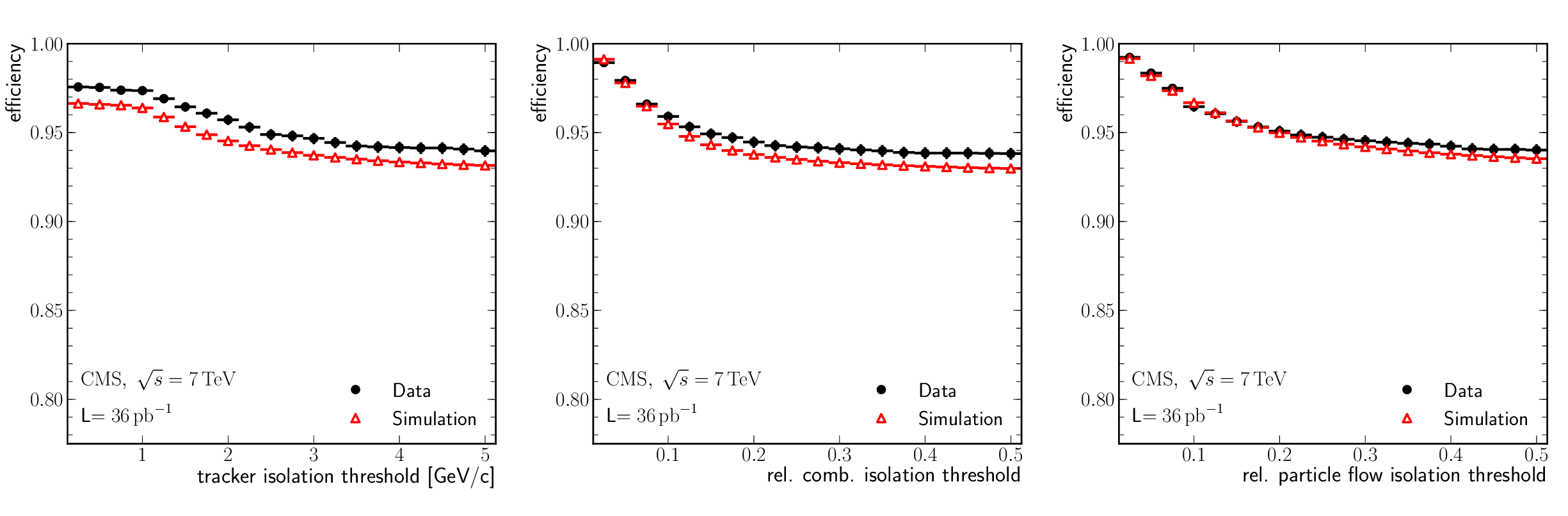
png pdf |
Figure 37:
Efficiency of single-muon trigger including isolation requirements for Tight Muons matched with the trigger objects passing trigger without isolation. Efficiencies measured in data (circles) are compared with the predictions of the MC simulation (triangles) as a function of the thresholds applied to the offline isolation variables: tracker absolute isolation (left), tracker-plus-calorimeters relative isolation (middle), and the particle-flow relative isolation (right). |
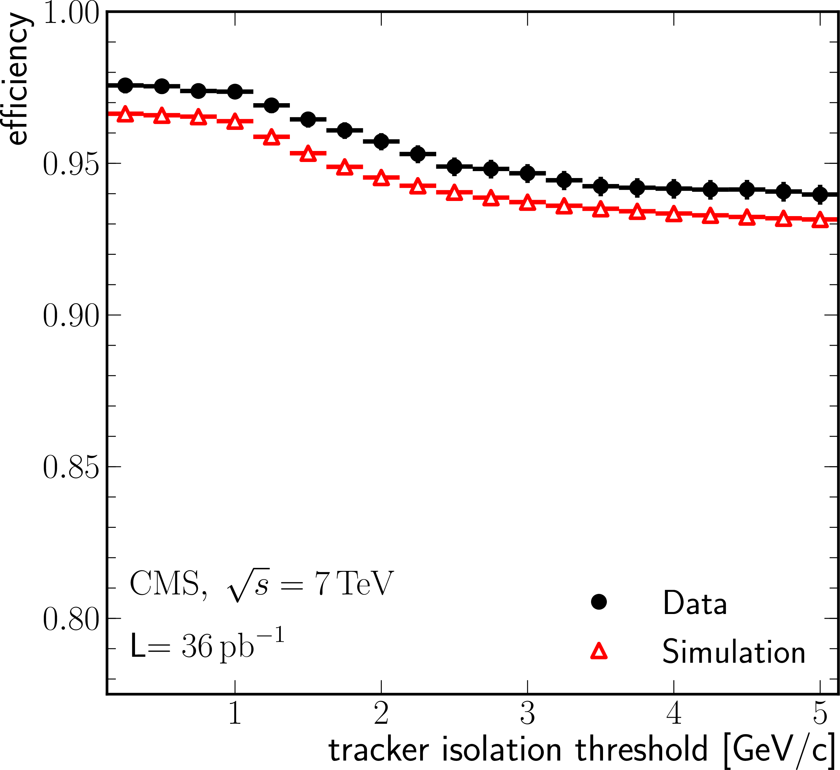
png pdf |
Figure 37-a:
Efficiency of single-muon trigger including isolation requirements for Tight Muons matched with the trigger objects passing trigger without isolation. Efficiencies measured in data (circles) are compared with the predictions of the MC simulation (triangles) as a function of the thresholds applied to the offline isolation variables: tracker absolute isolation (left), tracker-plus-calorimeters relative isolation (middle), and the particle-flow relative isolation (right). |
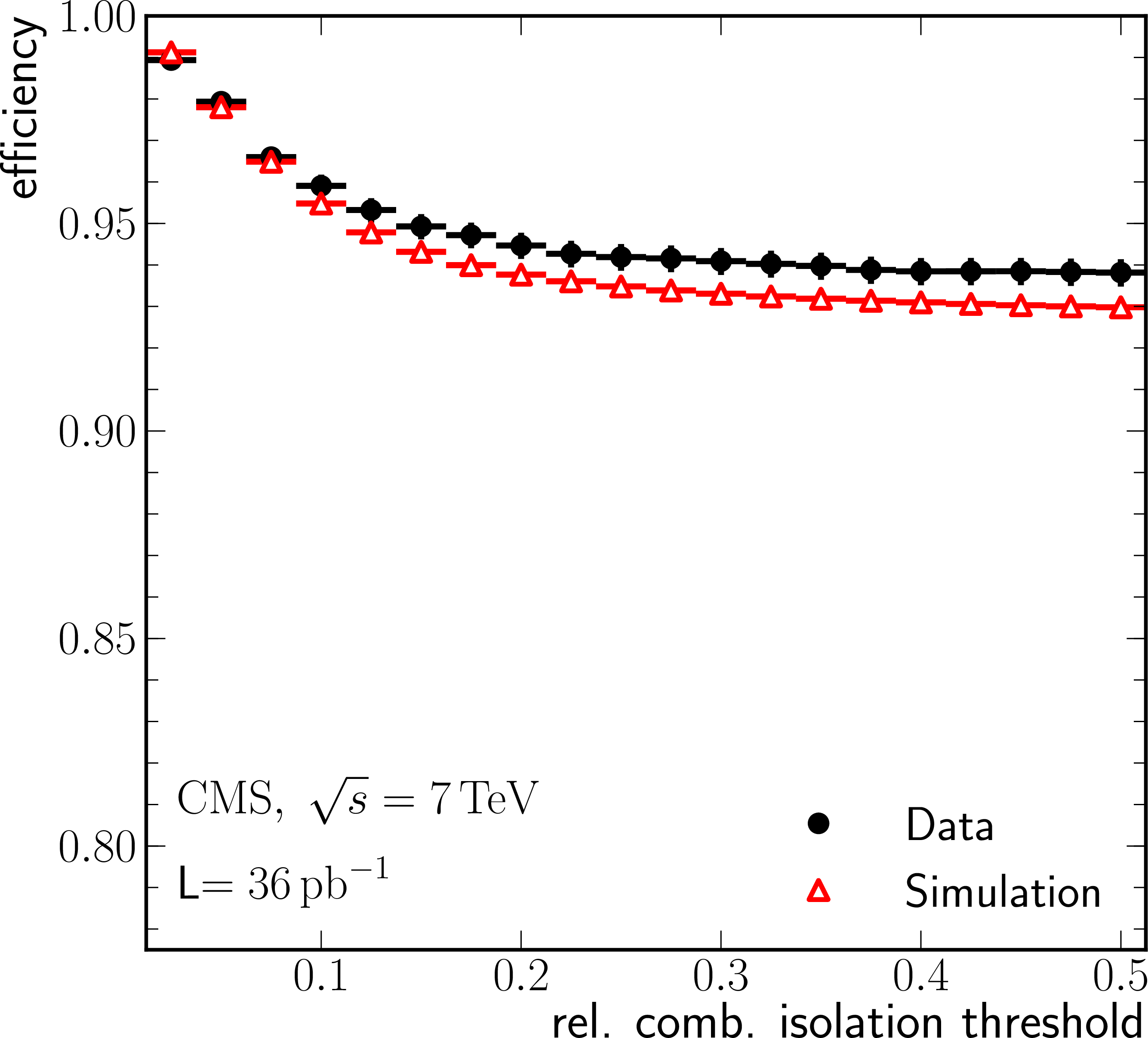
png pdf |
Figure 37-b:
Efficiency of single-muon trigger including isolation requirements for Tight Muons matched with the trigger objects passing trigger without isolation. Efficiencies measured in data (circles) are compared with the predictions of the MC simulation (triangles) as a function of the thresholds applied to the offline isolation variables: tracker absolute isolation (left), tracker-plus-calorimeters relative isolation (middle), and the particle-flow relative isolation (right). |

png pdf |
Figure 37-c:
Efficiency of single-muon trigger including isolation requirements for Tight Muons matched with the trigger objects passing trigger without isolation. Efficiencies measured in data (circles) are compared with the predictions of the MC simulation (triangles) as a function of the thresholds applied to the offline isolation variables: tracker absolute isolation (left), tracker-plus-calorimeters relative isolation (middle), and the particle-flow relative isolation (right). |
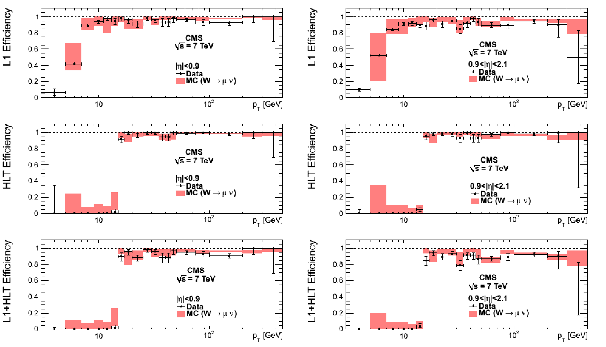
png pdf |
Figure 38:
Single-muon trigger efficiencies for Tight Muons passing the offline isolation selection as a function of the muon $ {p_{\mathrm {T}}} $, in the barrel ($|\eta |<0.9$, left) and the overlap-endcap ($0.9<|\eta |<2.1$, right) regions. In both regions the efficiencies for the following triggers are shown: the Level-1 trigger with $ {p_{\mathrm {T}}} $ threshold at 7 GeV/$c$ (top), the HLT with $ {p_{\mathrm {T}}} $ threshold at 15 GeV/$c$ with respect to the Level-1 (middle), and the combination of above Level-1 and HLT triggers (bottom). The efficiencies in data (points with error bars) are compared with predictions from the simulation ($\pm$1$\sigma$ bands); the uncertainties are statistical only. |
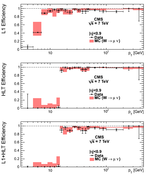
png |
Figure 38-a:
Single-muon trigger efficiencies for Tight Muons passing the offline isolation selection as a function of the muon $ {p_{\mathrm {T}}} $, in the barrel ($|\eta |<0.9$, left) and the overlap-endcap ($0.9<|\eta |<2.1$, right) regions. In both regions the efficiencies for the following triggers are shown: the Level-1 trigger with $ {p_{\mathrm {T}}} $ threshold at 7 GeV/$c$ (top), the HLT with $ {p_{\mathrm {T}}} $ threshold at 15 GeV/$c$ with respect to the Level-1 (middle), and the combination of above Level-1 and HLT triggers (bottom). The efficiencies in data (points with error bars) are compared with predictions from the simulation ($\pm$1$\sigma$ bands); the uncertainties are statistical only. |

png |
Figure 38-b:
Single-muon trigger efficiencies for Tight Muons passing the offline isolation selection as a function of the muon $ {p_{\mathrm {T}}} $, in the barrel ($|\eta |<0.9$, left) and the overlap-endcap ($0.9<|\eta |<2.1$, right) regions. In both regions the efficiencies for the following triggers are shown: the Level-1 trigger with $ {p_{\mathrm {T}}} $ threshold at 7 GeV/$c$ (top), the HLT with $ {p_{\mathrm {T}}} $ threshold at 15 GeV/$c$ with respect to the Level-1 (middle), and the combination of above Level-1 and HLT triggers (bottom). The efficiencies in data (points with error bars) are compared with predictions from the simulation ($\pm$1$\sigma$ bands); the uncertainties are statistical only. |
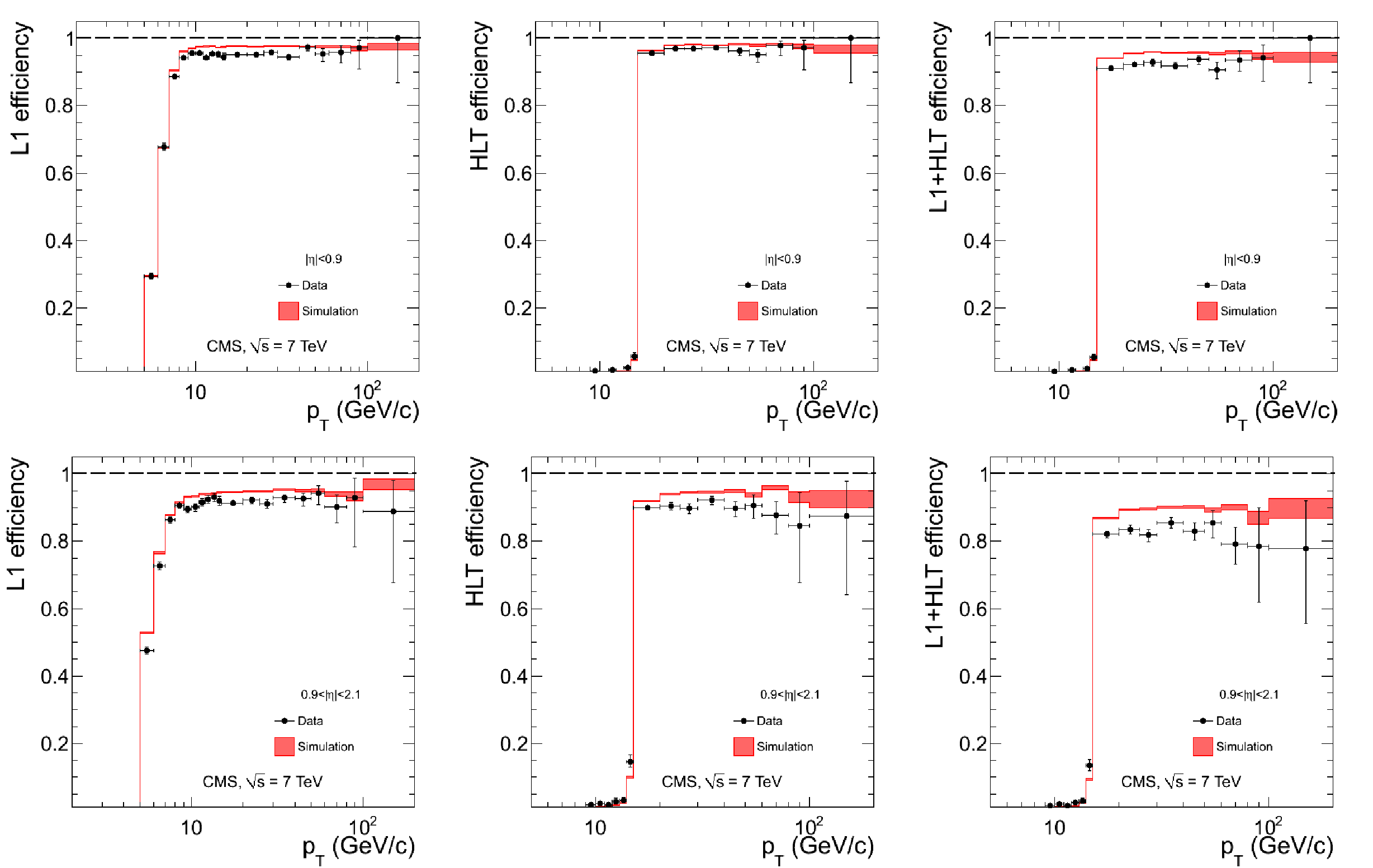
png pdf |
Figure 39:
Single-muon trigger efficiencies for Tight Muons contained in b-tagged jets as a function of the muon $ {p_{\mathrm {T}}} $, in the barrel (top) and the overlap-endcap (bottom) regions. The efficiencies are shown for the following triggers: the Level-1 trigger with $ {p_{\mathrm {T}}} $ threshold at 7 GeV/$c$ (left), the HLT with $ {p_{\mathrm {T}}} $ threshold at 15 GeV/$c$ with respect to the Level-1 (middle), and the combination of above Level-1 and HLT triggers (right). The efficiencies in data (points with error bars) are compared with predictions from the simulation ($\pm$1$\sigma$ bands); the uncertainties are statistical only. |

png |
Figure 39-a:
Single-muon trigger efficiencies for Tight Muons contained in b-tagged jets as a function of the muon $ {p_{\mathrm {T}}} $, in the barrel (top) and the overlap-endcap (bottom) regions. The efficiencies are shown for the following triggers: the Level-1 trigger with $ {p_{\mathrm {T}}} $ threshold at 7 GeV/$c$ (left), the HLT with $ {p_{\mathrm {T}}} $ threshold at 15 GeV/$c$ with respect to the Level-1 (middle), and the combination of above Level-1 and HLT triggers (right). The efficiencies in data (points with error bars) are compared with predictions from the simulation ($\pm$1$\sigma$ bands); the uncertainties are statistical only. |
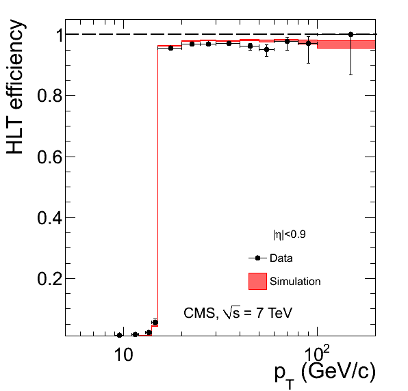
png |
Figure 39-b:
Single-muon trigger efficiencies for Tight Muons contained in b-tagged jets as a function of the muon $ {p_{\mathrm {T}}} $, in the barrel (top) and the overlap-endcap (bottom) regions. The efficiencies are shown for the following triggers: the Level-1 trigger with $ {p_{\mathrm {T}}} $ threshold at 7 GeV/$c$ (left), the HLT with $ {p_{\mathrm {T}}} $ threshold at 15 GeV/$c$ with respect to the Level-1 (middle), and the combination of above Level-1 and HLT triggers (right). The efficiencies in data (points with error bars) are compared with predictions from the simulation ($\pm$1$\sigma$ bands); the uncertainties are statistical only. |
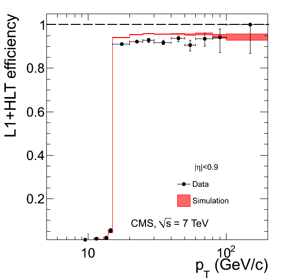
png |
Figure 39-c:
Single-muon trigger efficiencies for Tight Muons contained in b-tagged jets as a function of the muon $ {p_{\mathrm {T}}} $, in the barrel (top) and the overlap-endcap (bottom) regions. The efficiencies are shown for the following triggers: the Level-1 trigger with $ {p_{\mathrm {T}}} $ threshold at 7 GeV/$c$ (left), the HLT with $ {p_{\mathrm {T}}} $ threshold at 15 GeV/$c$ with respect to the Level-1 (middle), and the combination of above Level-1 and HLT triggers (right). The efficiencies in data (points with error bars) are compared with predictions from the simulation ($\pm$1$\sigma$ bands); the uncertainties are statistical only. |
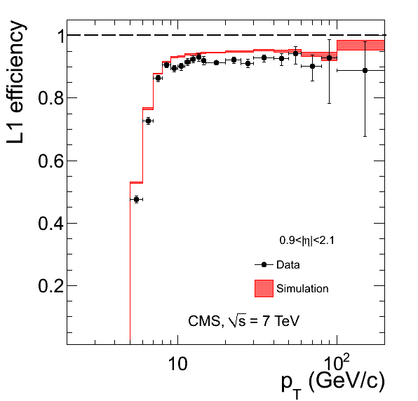
png |
Figure 39-d:
Single-muon trigger efficiencies for Tight Muons contained in b-tagged jets as a function of the muon $ {p_{\mathrm {T}}} $, in the barrel (top) and the overlap-endcap (bottom) regions. The efficiencies are shown for the following triggers: the Level-1 trigger with $ {p_{\mathrm {T}}} $ threshold at 7 GeV/$c$ (left), the HLT with $ {p_{\mathrm {T}}} $ threshold at 15 GeV/$c$ with respect to the Level-1 (middle), and the combination of above Level-1 and HLT triggers (right). The efficiencies in data (points with error bars) are compared with predictions from the simulation ($\pm$1$\sigma$ bands); the uncertainties are statistical only. |

png |
Figure 39-e:
Single-muon trigger efficiencies for Tight Muons contained in b-tagged jets as a function of the muon $ {p_{\mathrm {T}}} $, in the barrel (top) and the overlap-endcap (bottom) regions. The efficiencies are shown for the following triggers: the Level-1 trigger with $ {p_{\mathrm {T}}} $ threshold at 7 GeV/$c$ (left), the HLT with $ {p_{\mathrm {T}}} $ threshold at 15 GeV/$c$ with respect to the Level-1 (middle), and the combination of above Level-1 and HLT triggers (right). The efficiencies in data (points with error bars) are compared with predictions from the simulation ($\pm$1$\sigma$ bands); the uncertainties are statistical only. |

png |
Figure 39-f:
Single-muon trigger efficiencies for Tight Muons contained in b-tagged jets as a function of the muon $ {p_{\mathrm {T}}} $, in the barrel (top) and the overlap-endcap (bottom) regions. The efficiencies are shown for the following triggers: the Level-1 trigger with $ {p_{\mathrm {T}}} $ threshold at 7 GeV/$c$ (left), the HLT with $ {p_{\mathrm {T}}} $ threshold at 15 GeV/$c$ with respect to the Level-1 (middle), and the combination of above Level-1 and HLT triggers (right). The efficiencies in data (points with error bars) are compared with predictions from the simulation ($\pm$1$\sigma$ bands); the uncertainties are statistical only. |
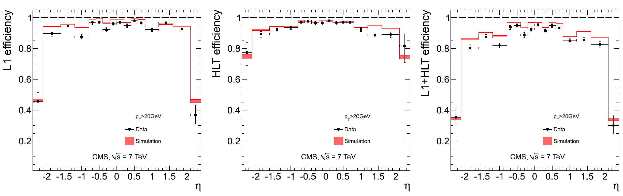
png pdf |
Figure 40:
Single-muon trigger efficiencies for Tight Muons contained in b-tagged jets as a function of the muon pseudorapidity, for muons with $ {p_{\mathrm {T}}} > $ 20GeV/$c$ : the efficiency of the Level-1 trigger with $ {p_{\mathrm {T}}} $ threshold at 7 GeV/$c$ (left), the efficiency of HLT with $ {p_{\mathrm {T}}} $ threshold at 15 GeV/$c$ with respect to the Level-1 (middle), and the combined efficiency of Level-1 and HLT (right). The efficiencies in data (points with error bars) are compared with predictions from the simulation ($\pm$1$\sigma$ bands); the uncertainties are statistical only. |

png |
Figure 40-a:
Single-muon trigger efficiencies for Tight Muons contained in b-tagged jets as a function of the muon pseudorapidity, for muons with $ {p_{\mathrm {T}}} > $ 20GeV/$c$ : the efficiency of the Level-1 trigger with $ {p_{\mathrm {T}}} $ threshold at 7 GeV/$c$ (left), the efficiency of HLT with $ {p_{\mathrm {T}}} $ threshold at 15 GeV/$c$ with respect to the Level-1 (middle), and the combined efficiency of Level-1 and HLT (right). The efficiencies in data (points with error bars) are compared with predictions from the simulation ($\pm$1$\sigma$ bands); the uncertainties are statistical only. |
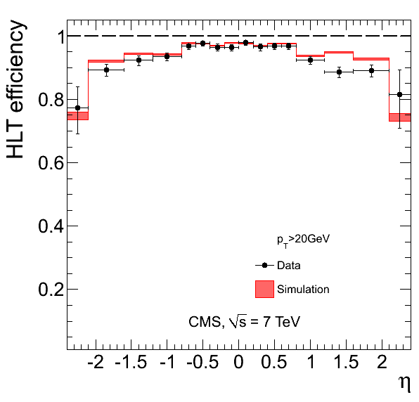
png |
Figure 40-b:
Single-muon trigger efficiencies for Tight Muons contained in b-tagged jets as a function of the muon pseudorapidity, for muons with $ {p_{\mathrm {T}}} > $ 20GeV/$c$ : the efficiency of the Level-1 trigger with $ {p_{\mathrm {T}}} $ threshold at 7 GeV/$c$ (left), the efficiency of HLT with $ {p_{\mathrm {T}}} $ threshold at 15 GeV/$c$ with respect to the Level-1 (middle), and the combined efficiency of Level-1 and HLT (right). The efficiencies in data (points with error bars) are compared with predictions from the simulation ($\pm$1$\sigma$ bands); the uncertainties are statistical only. |

png |
Figure 40-c:
Single-muon trigger efficiencies for Tight Muons contained in b-tagged jets as a function of the muon pseudorapidity, for muons with $ {p_{\mathrm {T}}} > $ 20GeV/$c$ : the efficiency of the Level-1 trigger with $ {p_{\mathrm {T}}} $ threshold at 7 GeV/$c$ (left), the efficiency of HLT with $ {p_{\mathrm {T}}} $ threshold at 15 GeV/$c$ with respect to the Level-1 (middle), and the combined efficiency of Level-1 and HLT (right). The efficiencies in data (points with error bars) are compared with predictions from the simulation ($\pm$1$\sigma$ bands); the uncertainties are statistical only. |
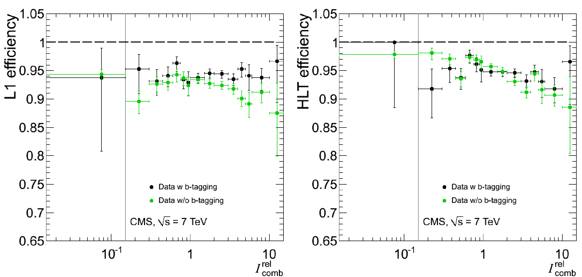
png pdf |
Figure 41:
Single-muon trigger efficiencies for Tight Muons with $ {p_{\mathrm {T}}} > $ 20 GeV/$c$ and $|\eta | < 2.1$, with and without the further b-tagging selection, as a function of the muon isolation variable $I^{\text {rel}}_{\text {comb}}$: the Level-1 trigger (left), and the HLT with respect to the Level-1 (right). |

png |
Figure 41-a:
Single-muon trigger efficiencies for Tight Muons with $ {p_{\mathrm {T}}} > $ 20 GeV/$c$ and $|\eta | < 2.1$, with and without the further b-tagging selection, as a function of the muon isolation variable $I^{\text {rel}}_{\text {comb}}$: the Level-1 trigger (left), and the HLT with respect to the Level-1 (right). |

png |
Figure 41-b:
Single-muon trigger efficiencies for Tight Muons with $ {p_{\mathrm {T}}} > $ 20 GeV/$c$ and $|\eta | < 2.1$, with and without the further b-tagging selection, as a function of the muon isolation variable $I^{\text {rel}}_{\text {comb}}$: the Level-1 trigger (left), and the HLT with respect to the Level-1 (right). |

png pdf |
Figure 42:
The accepted cross section of events as a function of muon trigger $ {p_{\mathrm {T}}} $ threshold for the actual Level-1 , Level-2 , and Level-3 muon trigger objects processed online in data, compared to the emulated Level-1 and HLT trigger in simulation. Points corresponding to thresholds of prescaled Level-3 triggers are not plotted. |
| Tables | |
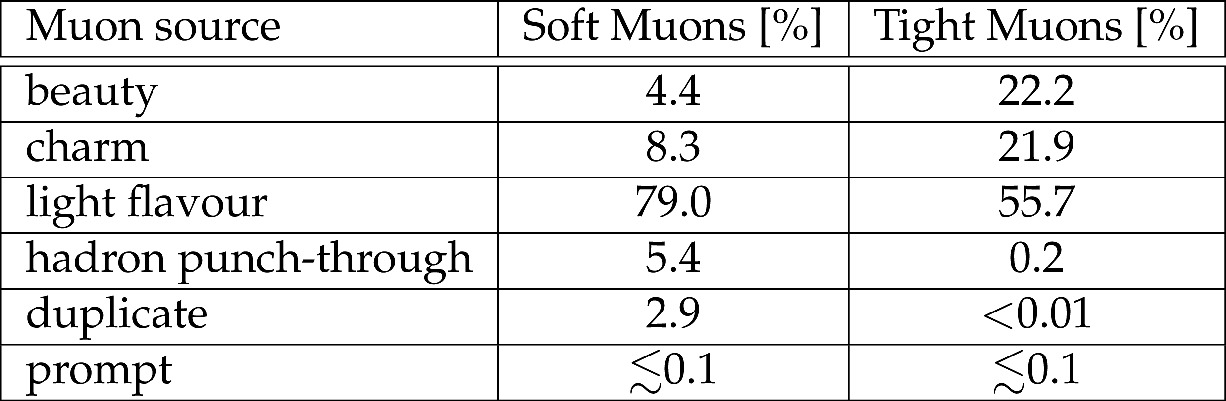
png pdf |
Table 1:
Composition by source of the low-$ {p_{\mathrm {T}}} $ muon candidates reconstructed in zero-bias events, according to simulation for the Soft and Tight Muon selections. |

png pdf |
Table 2:
Composition by source of Tight Muons with $ {p_{\mathrm {T}}} > $ 20 GeV/$c$ according to simulation. |

png pdf |
Table 3:
Muon efficiencies at the efficiency plateau for the different muon selections: efficiency measured from data, and ratio between the measurements in data and simulation. The first uncertainty quoted on the scale factor is the uncertainty on the efficiencies in data and simulation from the fitting procedure, which includes the statistical uncertainty; the second is from the additional systematic uncertainties described later in this section. |
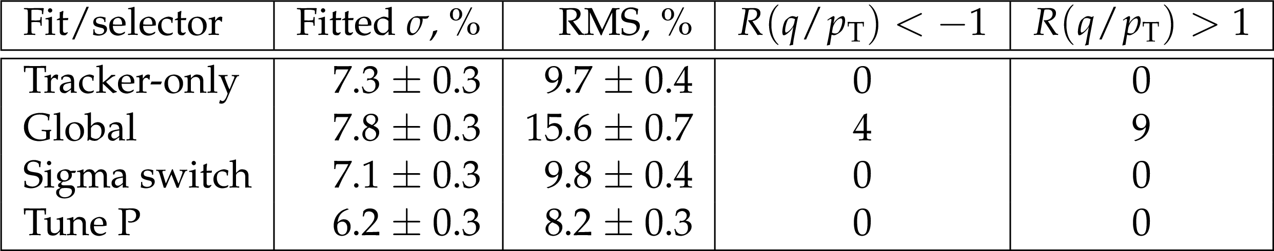
png pdf |
Table 4:
Comparison of the fitted Gaussian width $\sigma $, sample RMS (truncated at $\pm$1), and counts in the tails of the $R(q/ {p_{\mathrm {T}}} )$ distribution for 294 muons with measured transverse momentum in the range 350 $ < {p_{\mathrm {T}}} < $ 2000 GeV/$c$. |

png pdf |
Table 5:
The average $q/ {p_{\mathrm {T}}} $ bias obtained with the cosmic endpoint method in three bins of the azimuthal angle $\phi $ and for the whole studied $\phi $ range. The first uncertainty quoted is statistical; the second is systematic. Also shown are results obtained with the MuScleFit method (Section {sec:momentumScaleAtMediumPt}) by rescaling $ {p_{\mathrm {T}}} $ of each of the muons from ${\mathrm{ Z } } $ decays according to Eq.(\ref {eq:pdfMUSCLE}) and computing the average difference between the rescaled and the original $q/ {p_{\mathrm {T}}} $ values in bins of $\phi $. The distribution of muons from ${\mathrm{ Z } } $ decays was reweighted to have the same $\phi $ distribution as that of cosmic-ray muons. The uncertainty quoted is statistical only. |
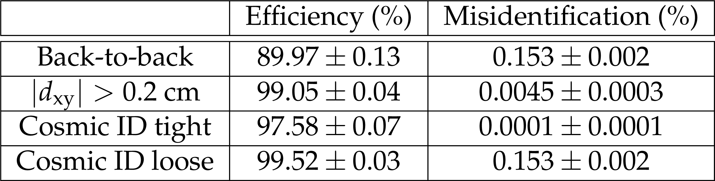
png pdf |
Table 6:
The efficiency of cosmic-ray muon identification and misidentification fractions for some relevant individual quantities and the loose and tight versions of the cosmic-muon identification algorithm. Uncertainties are statistical only. |

png pdf |
Table 7:
Level-1 , HLT, and overall single-muon trigger efficiencies for Soft Muons in the efficiency plateau (9 $ < {p_{\mathrm {T}}} < $ 20 GeV/$c$) for different pseudorapidity regions. The first column shows efficiencies measured from data; the second column shows the ratio between the measurements in data and simulation. The uncertainties are statistical only. |

png pdf |
Table 8:
Summary of Level-1 , HLT, and overall trigger efficiencies for Tight Muons at the efficiency plateau in different pseudorapidity regions. The results obtained using muons from ${\mathrm{ Z } } $ decays and single isolated muons collected with jet triggers are averaged over the $ {p_{\mathrm {T}}} $ range of 20-100 GeV/$c$ ; the results from single muons contained in b-tagged jets are reported without an upper $ {p_{\mathrm {T}}} $ limit. For each method, the first column shows efficiencies measured from data; the second column shows the ratios between the estimates in data and in simulation. The quoted uncertainties are purely statistical. |
| Summary |
| The performance of muon reconstruction, identification, and triggering in CMS has been studied extensively using 40 pb$^{-1}$ of data collected in pp collisions at $\sqrt{s} = $ 7 TeV at the LHC in 2010. These data were used to study several representative muon selections, which were chosen as benchmarks covering a wide range of physics analysis needs. The distributions of kinematic and identification variables for muons reconstructed from inclusive data samples are generally in good agreement with predictions from simulation over the momentum range of $p_{\mathrm{T}} < $ 200 GeV/$c$, including variables sensitive to large hit occupancies in the muon detectors. Identification efficiencies, for muons with $p_{\mathrm{T}}$ larger than a few GeV/$c$, are above 95% for all selections studied. They are correctly reproduced by the Monte Carlo simulations. Misidentification is lower than 1% for the loosest selection and below 0.1% for the tightest. In the specific case of several nearby muons, where the tightest selection becomes less efficient, an optimized selection was developed to preserve high efficiency with only a minimal increase of misidentification. Two complementary methods have been developed to evaluate muon momentum scale biases and resolution in the range 20 $ < p_{\mathrm{T}} < $ 100 GeV/$c$, where the momentum measurement is provided by the tracker. The average bias $\Delta(p_{\mathrm{T}})/p_{\mathrm{T}}$ in the muon momentum scale was measured with a precision of better than 0.2% and was found to be consistent with zero. The relative $p_{\mathrm{T}}$ resolution is between 1.3% to 2.0% for muons in the barrel and better than 6% in the endcaps, in good agreement with simulation. The transverse momentum resolution of tracks reconstructed using information from only muon detectors is better than 10% in the barrel region. At high momenta, the best measurement of muon $p_{\mathrm{T}}$ is obtained by selective use of information from the muon system in addition to that from the inner tracker. The $p_{\mathrm{T}}$ resolution, evaluated in the barrel region using muons from cosmic rays, is better than 10% up to 1 TeV/$c$. Algorithms to identify cosmic and beam-halo backgrounds among collision events were developed and successfully used in physics analyses of 2010 data. The performance of various muon isolation algorithms was shown to be reasonably well modelled by the simulation. The muon trigger efficiency for isolated muons is better than 90% over the full $\eta$ range, and is typically substantially better. In this document we have shown that the performance specifications set out for the measurement of muons in CMS have largely been met. The good performance and detailed understanding of the muon reconstruction, identification, and triggering provides the necessary confidence in all elements of the chain from muon detection to muon analysis, which is essential for searches for physics beyond the Standard Model as well as accurate Standard Model measurements. |
| References | ||||
| 1 | CMS Collaboration | Commissioning of the CMS experiment and the cosmic run at four tesla | JINST 5 (2010) T03001 | |
| 2 | CMS Collaboration | Performance of CMS muon reconstruction in cosmic-ray events | JINST 5 (2010) T03022 | CMS-CFT-09-014 0911.4994 |
| 3 | CMS Collaboration | Performance of muon identification in pp collisions at $ \sqrt{s} $ = 7 TeV | CDS | |
| 4 | CMS Collaboration | The CMS experiment at the CERN LHC | JINST 3 (2008) S08004 | CMS-00-001 |
| 5 | CMS Collaboration | The TriDAS Project Technical Design Report, volume I: The trigger systems | CDS | |
| 6 | CMS Collaboration | The TriDAS Project Technical Design Report, volume II: Data acquisition and high-level trigger | CDS | |
| 7 | J. Pumplin et al. | New generation of parton distributions with uncertainties from global QCD analysis | JHEP 07 (2002) 012 | |
| 8 | T. Sj\"ostrand, S. Mrenna, and P. Skands | PYTHIA 6.4 physics and manual | JHEP 05 (2006) 026 | |
| 9 | CMS Collaboration | Measurement of the underlying event activity at the LHC with $ \sqrt{s} = $ 7 TeV and comparison with $ \sqrt{s} = $ 0.9 TeV | JHEP 09 (2011) 109 | CMS-QCD-10-010 1107.0330 |
| 10 | D. J. Lange | The $ \textscEvtGen $ particle decay simulation package | NIMA 462 (2001) 152 | |
| 11 | S. Frixione, P. Nason, and C. Oleari | Matching NLO QCD computations with parton shower simulations: the POWHEG method | JHEP 11 (2007) 070 | 0709.2092 |
| 12 | J. Alwall et al. | MadGraph/MadEvent v4: the new web generation | JHEP 09 (2007) 028 | |
| 13 | GEANT4 Collaboration | GEANT4 --- a simulation toolkit | NIMA 506 (2003) 250 | |
| 14 | J. Allison et al. | Geant4 developments and applications | IEEE Trans. Nucl. Sci. 53 (2006) 270 | |
| 15 | CMS Collaboration | CMS Physics Technical Design Report, volume I: Detector performance and software | CDS | |
| 16 | R. Fr\"uhwirth | Application of Kalman filtering to track and vertex fitting | NIMA 262 (1987) 444 | |
| 17 | CMS Collaboration | Measurement of Tracking Efficiency | CDS | |
| 18 | CMS Collaboration | Prompt and non-prompt J/$ \psi $ production in pp collisions at $ \sqrt{s} = $ 7 TeV | EPJC 71 (2011) 1575 | |
| 19 | CMS Collaboration | Measurements of inclusive W and Z cross sections in pp collisions at $ \sqrt{s} = $ 7 TeV | JHEP 01 (2011) 080 | |
| 20 | CMS Collaboration | Measurement of the inclusive W and Z production cross sections in pp collisions at $ \sqrt{s} = $ 7 TeV with the CMS experiment | JHEP 10 (2011) 132 | CMS-EWK-10-005 1107.4789 |
| 21 | CMS Collaboration | Particle--Flow Event Reconstruction in CMS and Performance for Jets, Taus, and $ E_{\mathrm{T}}^{\text{miss}} $ | CDS | |
| 22 | CMS Collaboration | Commissioning of the particle-flow event reconstruction with leptons from J/$ \Psi $ and W decays at 7 TeV | CDS | |
| 23 | H. Burkhardt, M. Ferro-Luzzi, A. Macpherson, and M. Mangano, eds. | CERN, Geneva, (2011) | ||
| 24 | S. Frixione and B. R. Webber | Matching NLO QCD computations and parton shower simulations | JHEP 06 (2002) 029 | hep-ph/0204244 |
| 25 | S. Frixione, P. Nason, and B. R. Webber | Matching NLO QCD and parton showers in heavy flavour production | JHEP 08 (2003) 007 | hep-ph/0305252 |
| 26 | CMS Collaboration | Measurement of the B$ ^+ $ production cross section in pp collisions at $ \sqrt{s} = $ 7 TeV | PRL 106 (2011) 112001 | CMS-BPH-10-004 1101.0131 |
| 27 | CMS Collaboration | Measurement of the $ \PBz $ Production Cross Section in $ \mathrm{ p }\mathrm{ p } $ Collisions at $ \sqrt{s} = $ 7 TeV | PRL 106 (2011) 252001 | CMS-BPH-10-005 1104.2892 |
| 28 | M. J. Oreglia | PhD thesis, Stanford University, Stanford, U.S.A., 1980 SLAC-R-236 Appendix D | ||
| 29 | M. Pivk and F. R. Le Diberder | SPlot: A statistical tool to unfold data distributions | NIMA 555 (2005) 356 | physics/0402083 |
| 30 | N. Arkani-Hamed et al. | A theory of dark matter | PRD 79 (2009) 015014 | 0810.0713 |
| 31 | D. P. Finkbeiner and N. Weiner | Exciting dark matter and the INTEGRAL/SPI 511 keV signal | PRD 76 (2007) 083519 | astro-ph/0702587 |
| 32 | D. Smith and N. Weiner | Inelastic dark matter | PRD 64 (2001) 043502 | hep-ph/0101138 |
| 33 | PAMELA Collaboration | An anomalous positron abundance in cosmic rays with energies 1.5--100$ GeV $ | Nature 458 (2009) 607 | 0810.4995 |
| 34 | Fermi LAT Collaboration | Measurement of the cosmic ray $ e^{+} + e^{-} $ spectrum from 20$ GeV $ to 1$ TeV $ with the Fermi Large Area Telescope | PRL 102 (2009) 181101 | 0905.0025 |
| 35 | J. Chang et al. | An excess of cosmic ray electrons at energies of 300--800$ GeV $ | Nature 456 (2008) 362 | |
| 36 | CMS Collaboration | Tracking and vertexing results from first collisions | EPJC 70 (2010) 165 | |
| 37 | CMS Collaboration | Measurement of Momentum Scale and Resolution using Low-mass Resonances and Cosmic Ray Muons | CDS | |
| 38 | S. Dittmaier and M. Huber | Radiative corrections to the neutral-current Drell--Yan process in the Standard Model and its minimal supersymmetric extension | JHEP 01 (2010) 060 | 0911.2329 |
| 39 | CMS Collaboration | Measurement of the charge asymmetry of atmospheric muons with the CMS detector | CDS | |
| 40 | CMS Collaboration | Search for a W' boson decaying to a muon and a neutrino in pp collisions at $ \sqrt{s} = $ 7 TeV | PLB 701 (2011) 160 | CMS-EXO-10-015 1103.0030 |
| 41 | CMS Collaboration | Search for resonances in the dilepton mass distribution in pp collisions at $ \sqrt{s} = $ 7 TeV | JHEP 05 (2011) 093 | CMS-EXO-10-013 1103.0981 |
| 42 | CMS Collaboration | Missing transverse energy performance of the CMS detector | JINST 6 (2011) P09001 | CMS-JME-10-009 1106.5048 |
| 43 | CMS Collaboration | Search for stopped gluinos in pp collisions at $ \sqrt{s} = $ 7 TeV | PRL 106 (2011) 011801 | CMS-EXO-10-003 1011.5861 |
| 44 | CMS Collaboration | Search for new physics with jets and missing transverse momentum in pp collisions at $ \sqrt{s} = $ 7 TeV | JHEP 08 (2011) 155 | CMS-SUS-10-005 1106.4503 |
| 45 | CMS Collaboration | Measurement of the inclusive Z cross section via decays to tau pairs in pp collisions at $ \sqrt{s} = $ 7 TeV | JHEP 08 (2011) 117 | CMS-EWK-10-013 1104.1617 |
| 46 | CMS Collaboration | Search for neutral minimal supersymmetric Standard Model Higgs bosons decaying to tau pairs in pp collisions at $ \sqrt{s} = $ 7 TeV | PRL 106 (2011) 231801 | CMS-TRK-10-001 1007.1988 |
| 47 | S. Abdullin et al. | Sensitivity of the muon isolation cut efficiency to the underlying event uncertainties | CMS Note 2006-033 | |
| 48 | M. Cacciari and G. P. Salam | Pileup subtraction using jet areas | PLB 659 (2008) 119 | 0707.1378 |
| 49 | CMS Collaboration | The performance of the CMS muon detector using pp collisions at $ \sqrt{s} = $ 7 TeV at the LHC | ||
| 50 | CMS Collaboration | Performance of b-jet identification in CMS | CDS | |
|
|
Compact Muon Solenoid LHC, CERN |
|

|

|

|

|

|