

Compact Muon Solenoid
LHC, CERN
| CMS-SUS-15-002 ; CERN-EP-2016-036 | ||
| Search for supersymmetry in the multijet and missing transverse momentum final state in pp collisions at 13 TeV | ||
| CMS Collaboration | ||
| 21 February 2016 | ||
| Phys. Lett. B 758 (2016) 152 | ||
| Abstract: A search for new physics is performed based on all-hadronic events with large missing transverse momentum produced in proton-proton collisions at $\sqrt{s}=$ 13 TeV. The data sample, corresponding to an integrated luminosity of 2.3 fb$^{-1}$, was collected with the CMS detector at the CERN LHC in 2015. The data are examined in search regions of jet multiplicity, tagged bottom quark jet multiplicity, missing transverse momentum, and the scalar sum of jet transverse momenta. The observed numbers of events in all search regions are found to be consistent with the expectations from standard model processes. Exclusion limits are presented for simplified supersymmetric models of gluino pair production. Depending on the assumed gluino decay mechanism, and for a massless, weakly interacting, lightest neutralino, lower limits on the gluino mass from 1440 to 1600 GeV are obtained, significantly extending previous limits. | ||
| Links: e-print arXiv:1602.06581 [hep-ex] (PDF) ; CDS record ; inSPIRE record ; HepData record ; CADI line (restricted) ; | ||
| Figures | |

png pdf |
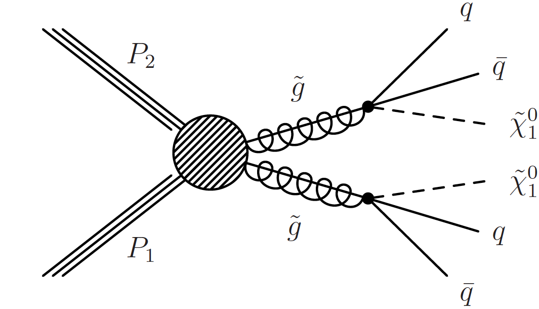
Figure 1-a:
Event diagrams for the new-physics scenarios considered in this study: the T1bbbb simplified model. |
png pdf |
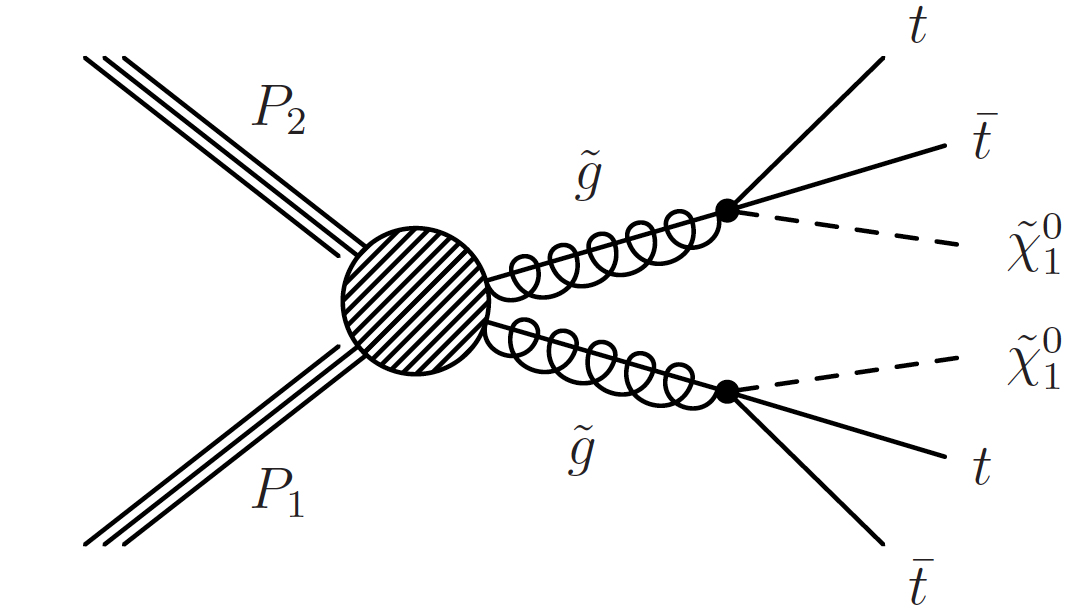
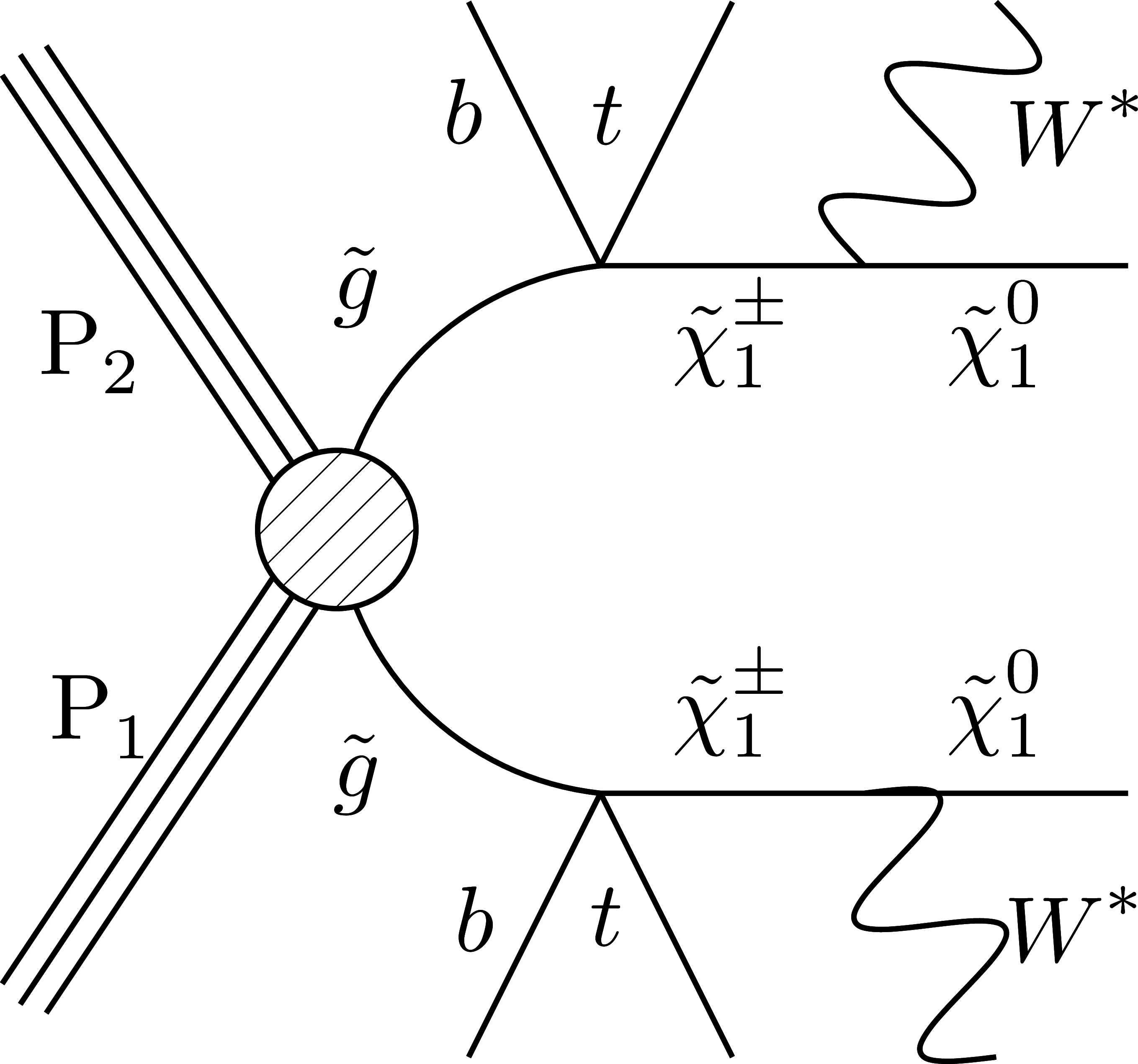
Figure 1-b:
Event diagrams for the new-physics scenarios considered in this study: the T1tttt simplified model. |
png pdf |
Figure 1-c:
Event diagrams for the new-physics scenarios considered in this study: the T1qqqq simplified model. |
png pdf |
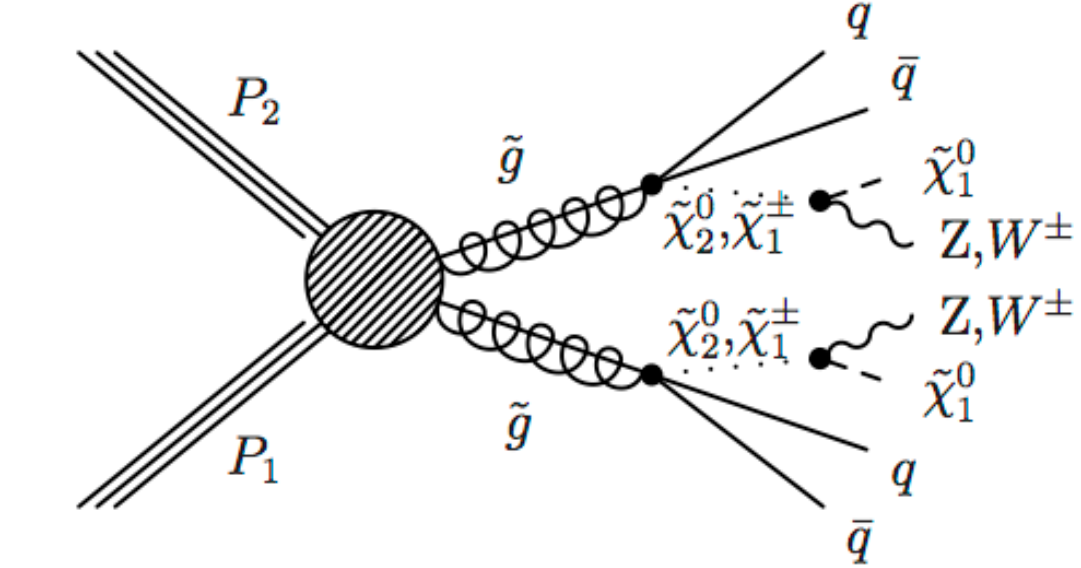
Figure 1-d:
Event diagrams for the new-physics scenarios considered in this study: the T5qqqqVV simplified model. |

png pdf |
Figure 2:
Schematic illustration of the search intervals in the $ {H_{\mathrm T}^{\text {miss}}} $ versus $ {H_{\mathrm {T}}} $ plane. Each of the six ${H_{\mathrm {T}}} $ and $ {H_{\mathrm T}^{\text {miss}}} $ intervals is examined in three $ {N_{\text {jet}}} $ and four $ {N_{{\mathrm{ b } }\text {-jet}}} $ bins for a total of 72 search regions. |
png pdf |
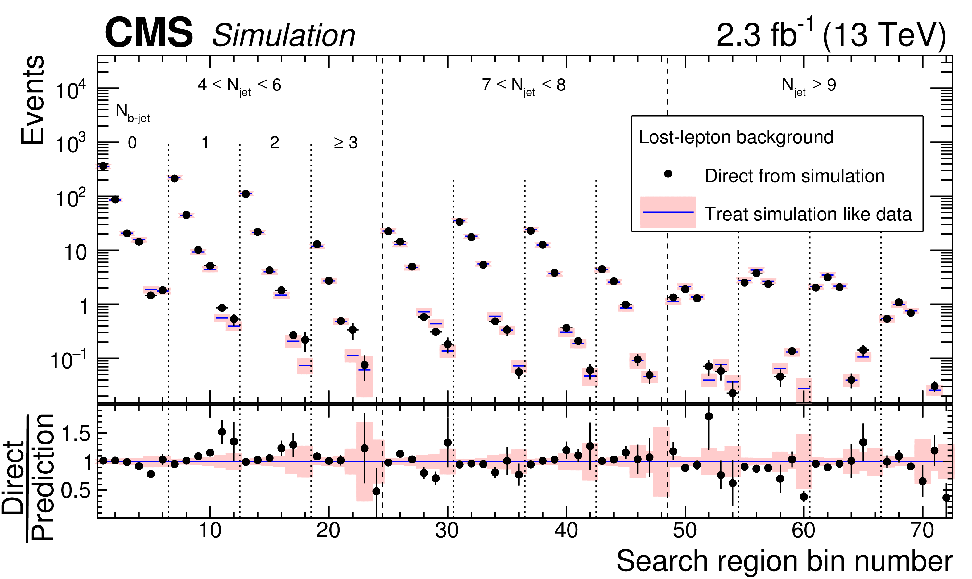
Figure 3-a:
(a) The lost-lepton background in the 72 search regions of the analysis as determined directly from $\mathrm{ t \bar{t} }$, single top quark, ${\mathrm{ W }+jets} $, diboson, and rare-event simulation (points, with statistical uncertainties) and as predicted by applying the lost-lepton background determination procedure to simulated electron and muon control samples (histograms, with statistical uncertainties). The lower panel shows the same results following division by the predicted value. (b) The corresponding simulated results for the background from hadronically decaying $\tau $ leptons. For both plots, the six results within each region delineated by dashed lines correspond sequentially to the six regions of $ {H_{\mathrm {T}}} $ and $ {H_{\mathrm T}^{\text {miss}}} $ indicated in Fig.2. Bins without markers have no events in the control regions. |

png pdf |
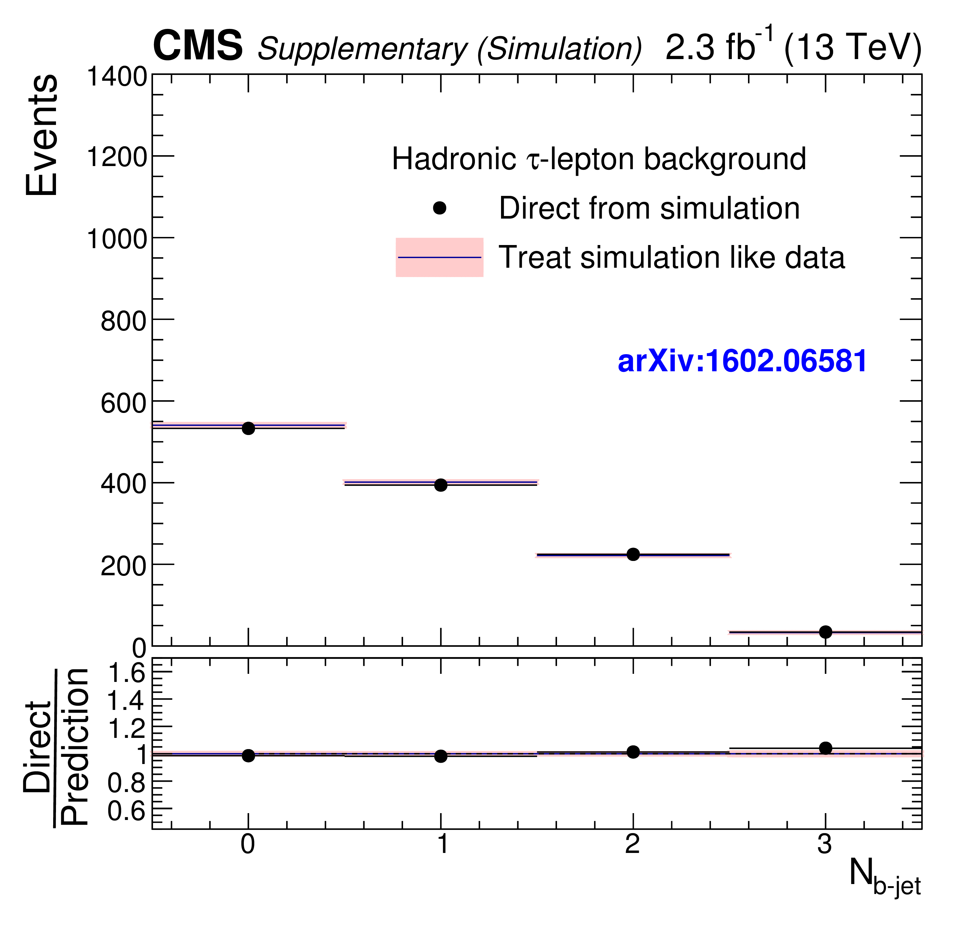
Figure 3-b:
(a) The lost-lepton background in the 72 search regions of the analysis as determined directly from $\mathrm{ t \bar{t} }$, single top quark, ${\mathrm{ W }+jets} $, diboson, and rare-event simulation (points, with statistical uncertainties) and as predicted by applying the lost-lepton background determination procedure to simulated electron and muon control samples (histograms, with statistical uncertainties). The lower panel shows the same results following division by the predicted value. (b) The corresponding simulated results for the background from hadronically decaying $\tau $ leptons. For both plots, the six results within each region delineated by dashed lines correspond sequentially to the six regions of $ {H_{\mathrm {T}}} $ and $ {H_{\mathrm T}^{\text {miss}}} $ indicated in Fig.2. Bins without markers have no events in the control regions. |

png pdf |
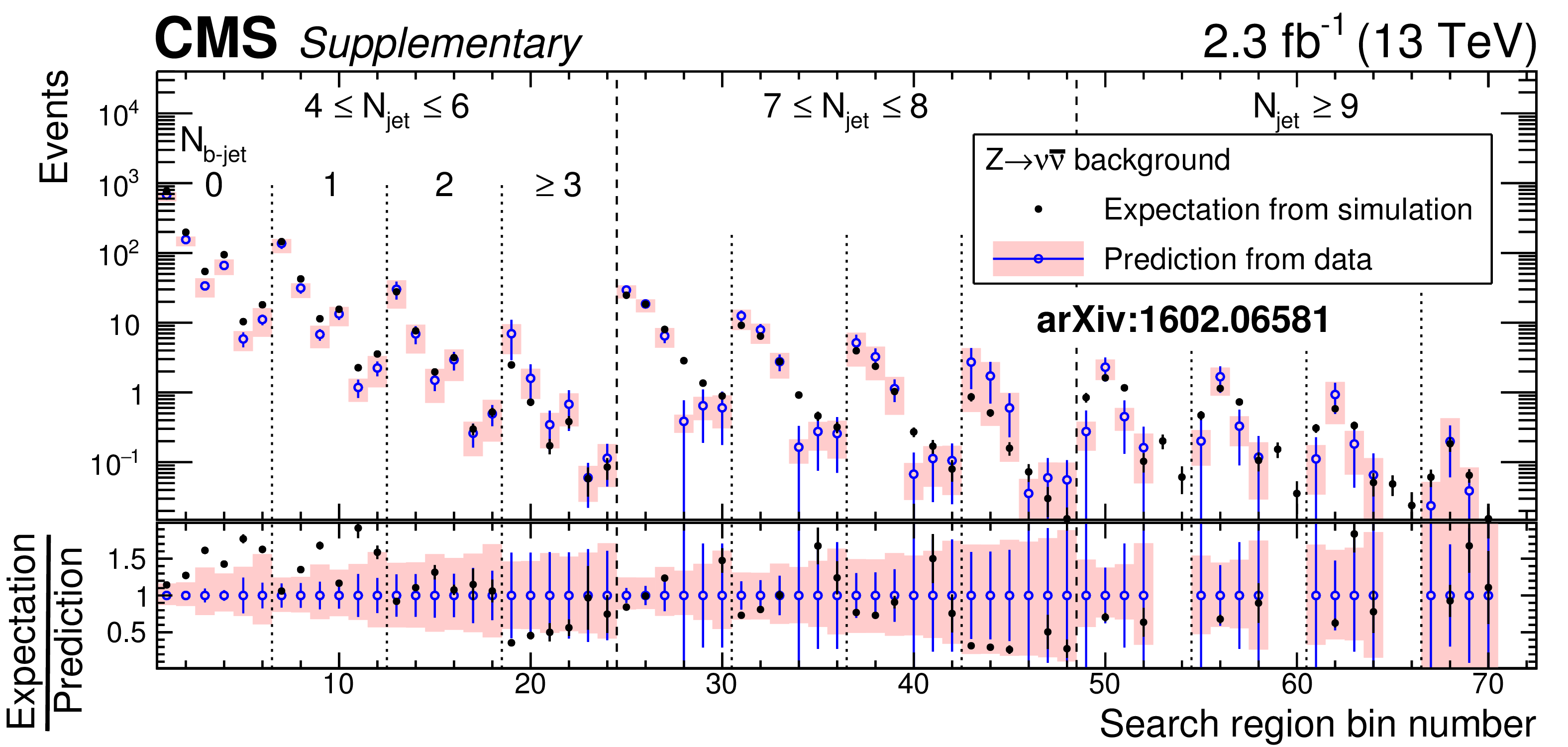
Figure 4:
The $ \mathrm{ Z } \to \nu \bar{\nu} $ background in the 72 search regions of the analysis as determined directly from $ \mathrm{Z} (\to \nu \bar{\nu} )$+jets and $\mathrm{ t \bar{t} Z } $ simulation (points), and as predicted by applying the $ \mathrm{ Z } \to \nu \bar{\nu}$ background determination procedure to statistically independent $ {\mathrm{ Z } (\to \ell ^{+} \ell ^{-} )}$+jets simulated event samples (histogram). For bins corresponding to $ {N_{{\mathrm{ b } }\text {-jet}}} =$ 0, the agreement is exact by construction. The lower panel shows the ratio between the true and predicted yields. For both the upper and lower panels, the shaded regions indicate the quadrature sum of the systematic uncertainty associated with the dependence of $\mathcal {F}$ on the kinematic parameters ($ {H_{\mathrm {T}}} $ and $ {H_{\mathrm T}^{\text {miss}}} $) and the statistical uncertainty of the simulated sample. The labeling of the search regions is the same as in Fig.3. |

png pdf |
Figure 5:
The QCD multijet background in the 72 search regions of the analysis as determined directly from QCD multijet simulation (points, with statistical uncertainties) and as predicted by applying the QCD multijet background determination procedure to simulated event samples (histograms, with statistical and systematic uncertainties added in quadrature). The lower panel shows the same results following division by the predicted value. The labeling of the search regions is the same as in Fig.3. Bins without markers have no events in the control regions. |
png pdf |
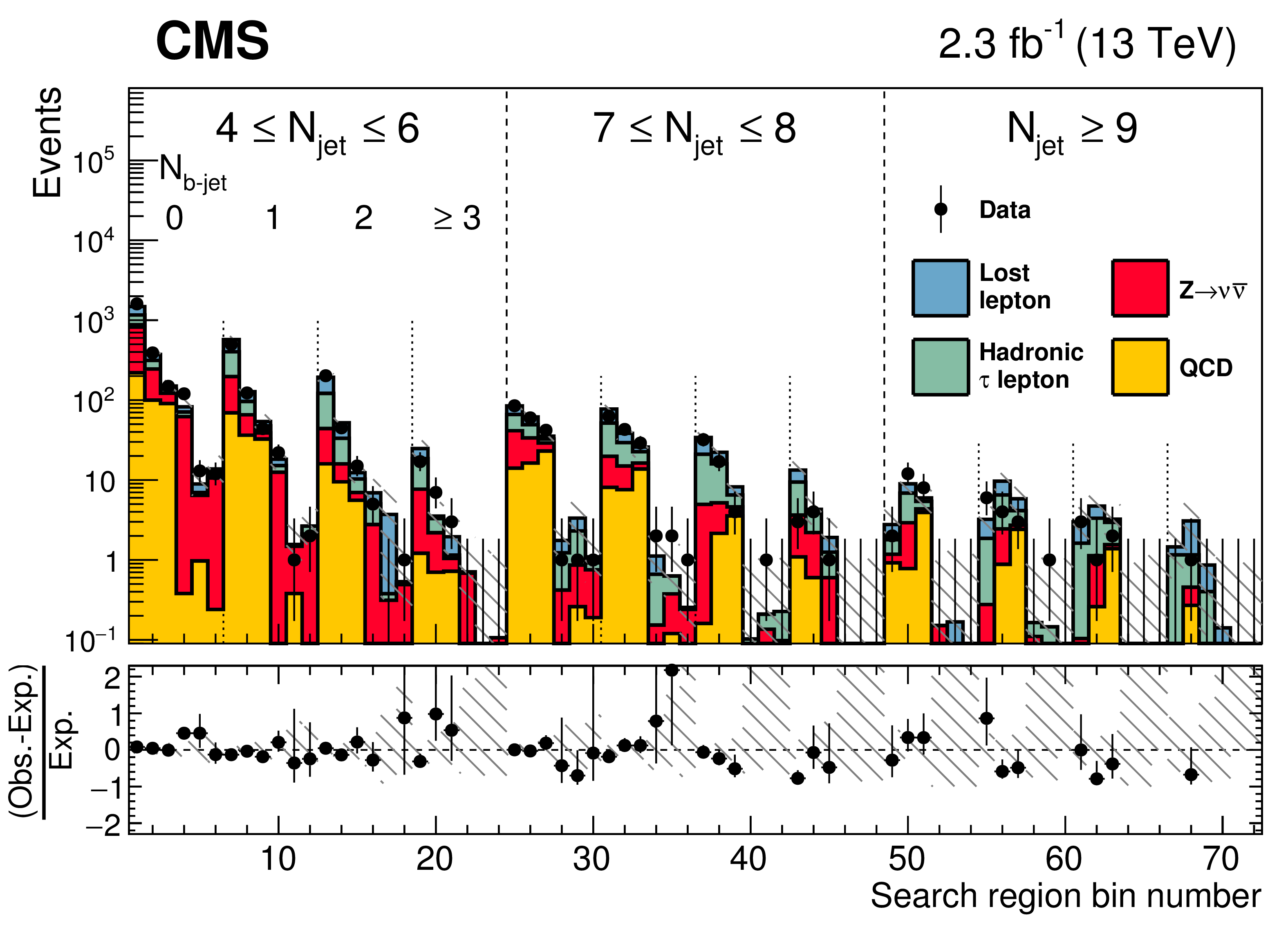
Figure 6:
Observed numbers of events and corresponding SM background predictions in the 72 search regions of the analysis, with fractional differences shown in the lower panel. The shaded regions indicate the total uncertainties in the background predictions. The labeling of the search regions is the same as in Fig.3. |
png pdf |
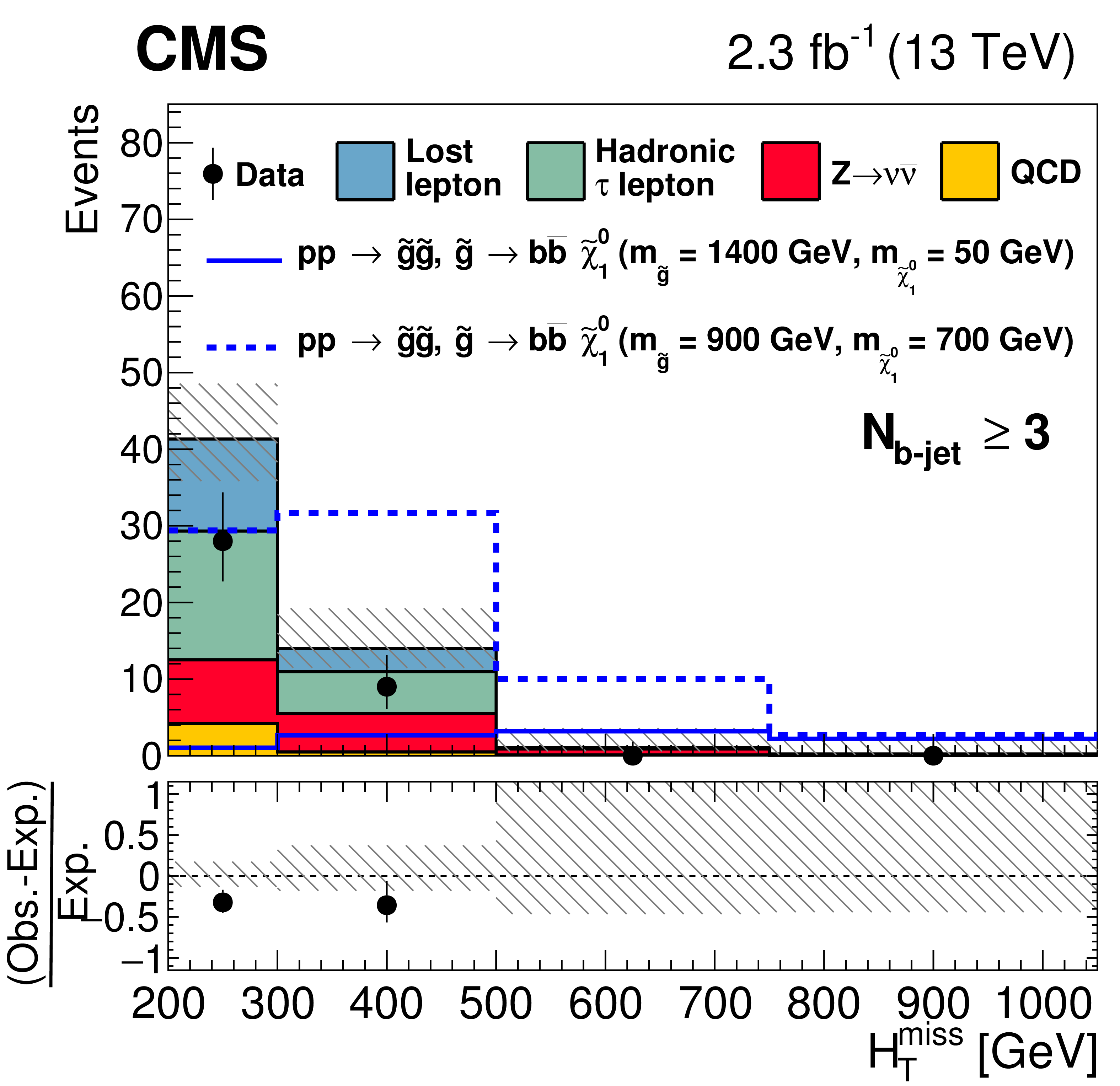
Figure 7-a:
Observed numbers of events and corresponding SM background predictions for intervals of the search region parameter space particularly sensitive to the (a) T1bbbb, (b) T1tttt, (c) T1qqqq, and (d) T5qqqqVV scenarios. The selection requirements are given in the figure legends. The hatched regions indicate the total uncertainties in the background predictions. The (unstacked) results for two example signal scenarios are shown in each instance, one with ${ {m_{\tilde{g} }} }\gg {m_{{\tilde{\chi}^0 }_1}} $ and the other with ${ {m_{{\tilde{\chi}^0 }_1}} }\sim {m_{\tilde{g} }} $. Note that for purposes of presentation, the four-bin scheme discussed in Section 5.3 is used for the $ {H_{\mathrm T}^{\text {miss}}} $ variable. |
png pdf |
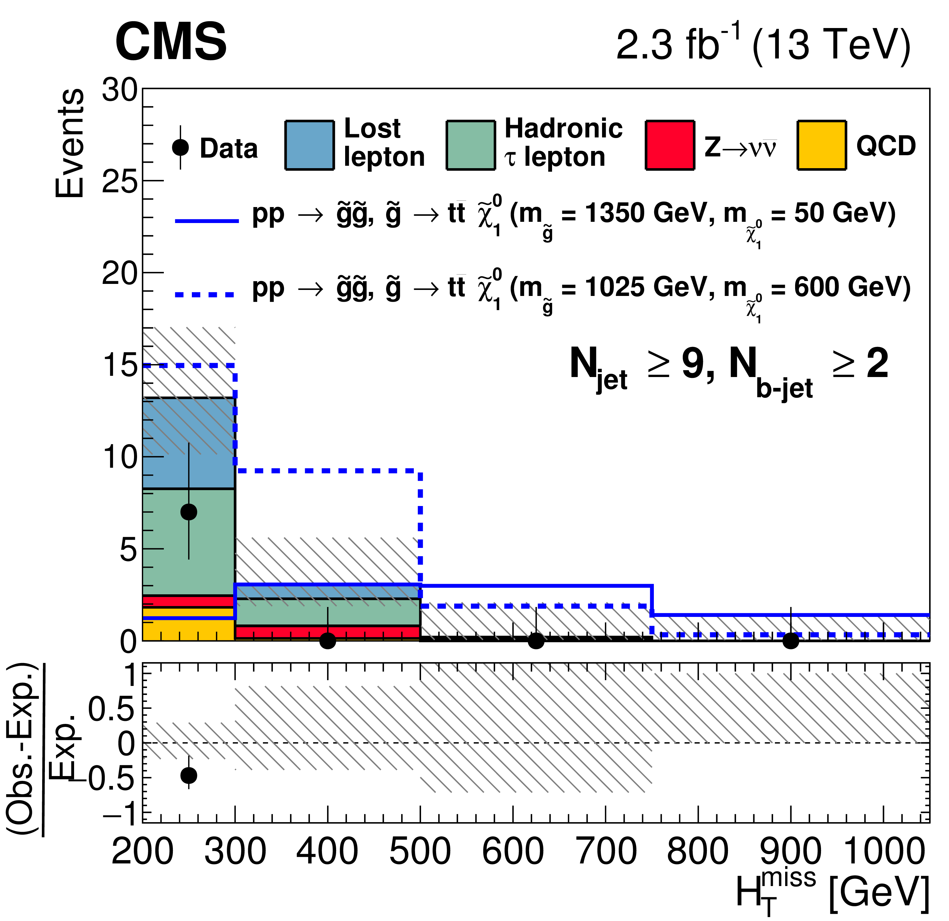
Figure 7-b:
Observed numbers of events and corresponding SM background predictions for intervals of the search region parameter space particularly sensitive to the (a) T1bbbb, (b) T1tttt, (c) T1qqqq, and (d) T5qqqqVV scenarios. The selection requirements are given in the figure legends. The hatched regions indicate the total uncertainties in the background predictions. The (unstacked) results for two example signal scenarios are shown in each instance, one with ${ {m_{\tilde{g} }} }\gg {m_{{\tilde{\chi}^0 }_1}} $ and the other with ${ {m_{{\tilde{\chi}^0 }_1}} }\sim {m_{\tilde{g} }} $. Note that for purposes of presentation, the four-bin scheme discussed in Section 5.3 is used for the $ {H_{\mathrm T}^{\text {miss}}} $ variable. |
png pdf |
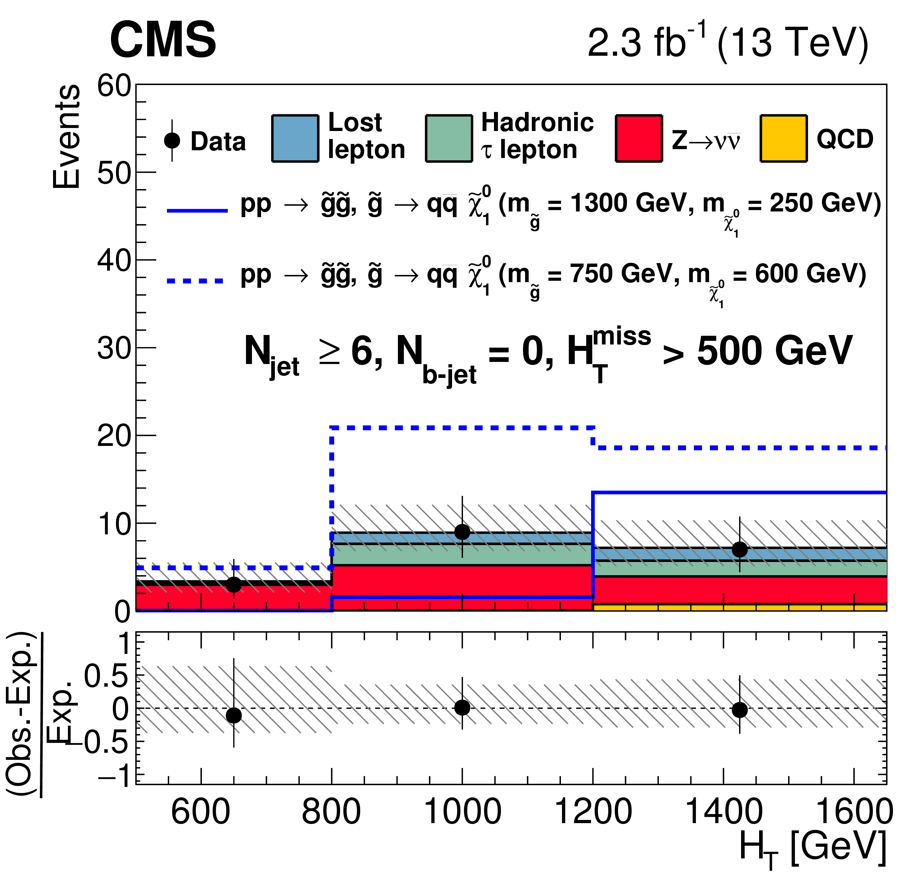
Figure 7-c:
Observed numbers of events and corresponding SM background predictions for intervals of the search region parameter space particularly sensitive to the (a) T1bbbb, (b) T1tttt, (c) T1qqqq, and (d) T5qqqqVV scenarios. The selection requirements are given in the figure legends. The hatched regions indicate the total uncertainties in the background predictions. The (unstacked) results for two example signal scenarios are shown in each instance, one with ${ {m_{\tilde{g} }} }\gg {m_{{\tilde{\chi}^0 }_1}} $ and the other with ${ {m_{{\tilde{\chi}^0 }_1}} }\sim {m_{\tilde{g} }} $. Note that for purposes of presentation, the four-bin scheme discussed in Section 5.3 is used for the $ {H_{\mathrm T}^{\text {miss}}} $ variable. |

png pdf |
Figure 7-d:
Observed numbers of events and corresponding SM background predictions for intervals of the search region parameter space particularly sensitive to the (a) T1bbbb, (b) T1tttt, (c) T1qqqq, and (d) T5qqqqVV scenarios. The selection requirements are given in the figure legends. The hatched regions indicate the total uncertainties in the background predictions. The (unstacked) results for two example signal scenarios are shown in each instance, one with ${ {m_{\tilde{g} }} }\gg {m_{{\tilde{\chi}^0 }_1}} $ and the other with ${ {m_{{\tilde{\chi}^0 }_1}} }\sim {m_{\tilde{g} }} $. Note that for purposes of presentation, the four-bin scheme discussed in Section 5.3 is used for the $ {H_{\mathrm T}^{\text {miss}}} $ variable. |
png pdf root |
Figure 8-a:
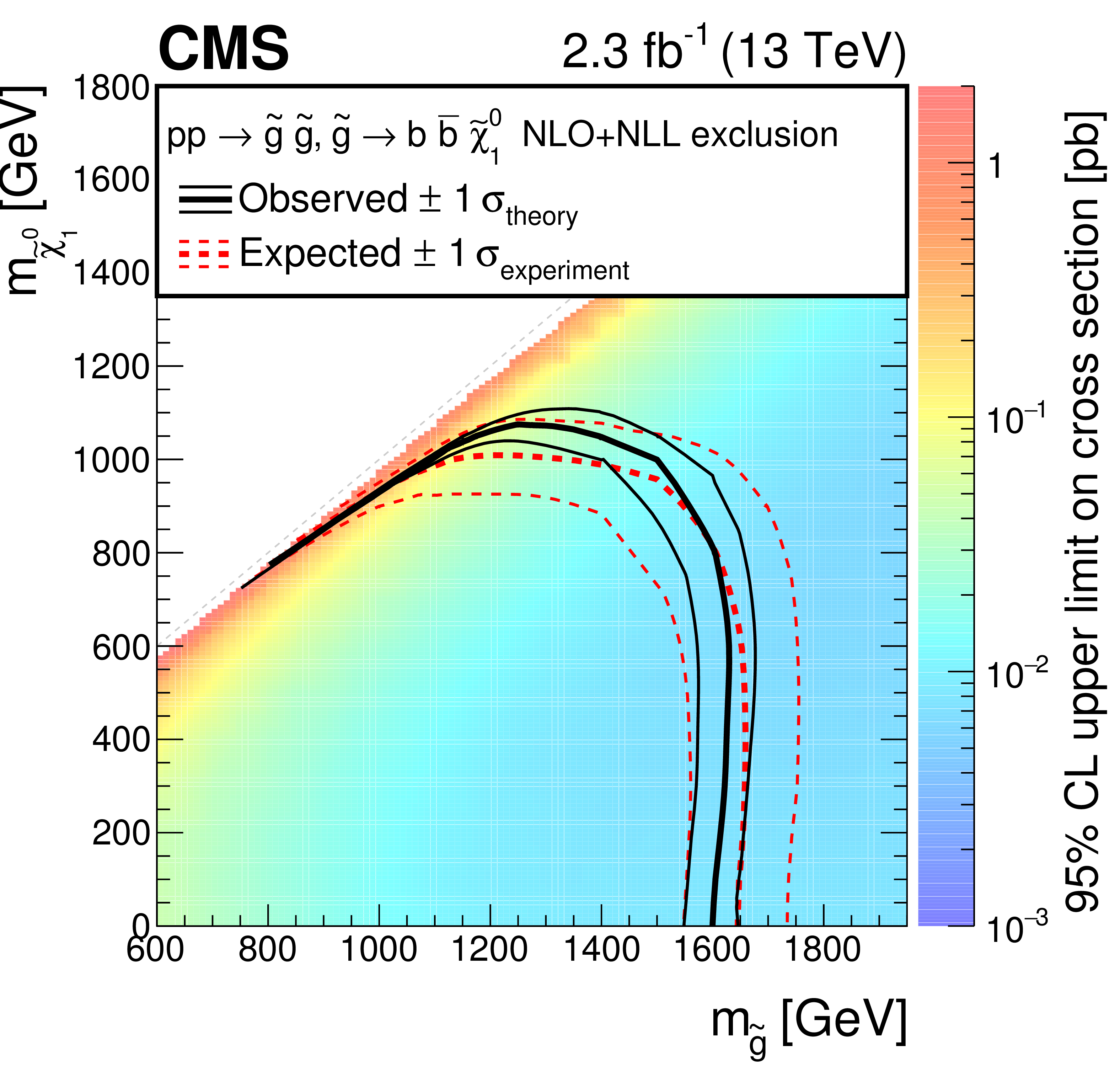
The 95% CL upper limits on the production cross sections for the (a) T1bbbb, (b) T1tttt, (c) T1qqqq, and (d) T5qqqqVV simplified models of supersymmetry, shown as a function of the gluino and LSP masses $ {m_{\tilde{g} }} $ and $ {m_{{\tilde{\chi}^0 }_1}} $. For the T5qqqqVV model, the masses of the intermediate $\tilde{\chi}^0_2$ and $\tilde{\chi}^{\pm} _1$ states are taken to be the mean of $ {m_{{\tilde{\chi}^0 }_1}} $ and $ {m_{\tilde{g} }} $. The solid (black) curves show the observed exclusion contours assuming the NLO+NLL cross sections [55-59], with the corresponding $\pm $1standard deviation uncertainties [75]. The dashed (red) curves present the expected limits with $\pm $1 standard deviation experimental uncertainties. The diagonal dashed (grey) lines indicate the kinematic limits of the respective decay. |

png pdf root |
Figure 8-b:
The 95% CL upper limits on the production cross sections for the (a) T1bbbb, (b) T1tttt, (c) T1qqqq, and (d) T5qqqqVV simplified models of supersymmetry, shown as a function of the gluino and LSP masses $ {m_{\tilde{g} }} $ and $ {m_{{\tilde{\chi}^0 }_1}} $. For the T5qqqqVV model, the masses of the intermediate $\tilde{\chi}^0_2$ and $\tilde{\chi}^{\pm} _1$ states are taken to be the mean of $ {m_{{\tilde{\chi}^0 }_1}} $ and $ {m_{\tilde{g} }} $. The solid (black) curves show the observed exclusion contours assuming the NLO+NLL cross sections [55-59], with the corresponding $\pm $1standard deviation uncertainties [75]. The dashed (red) curves present the expected limits with $\pm $1 standard deviation experimental uncertainties. The diagonal dashed (grey) lines indicate the kinematic limits of the respective decay. |
png pdf root |
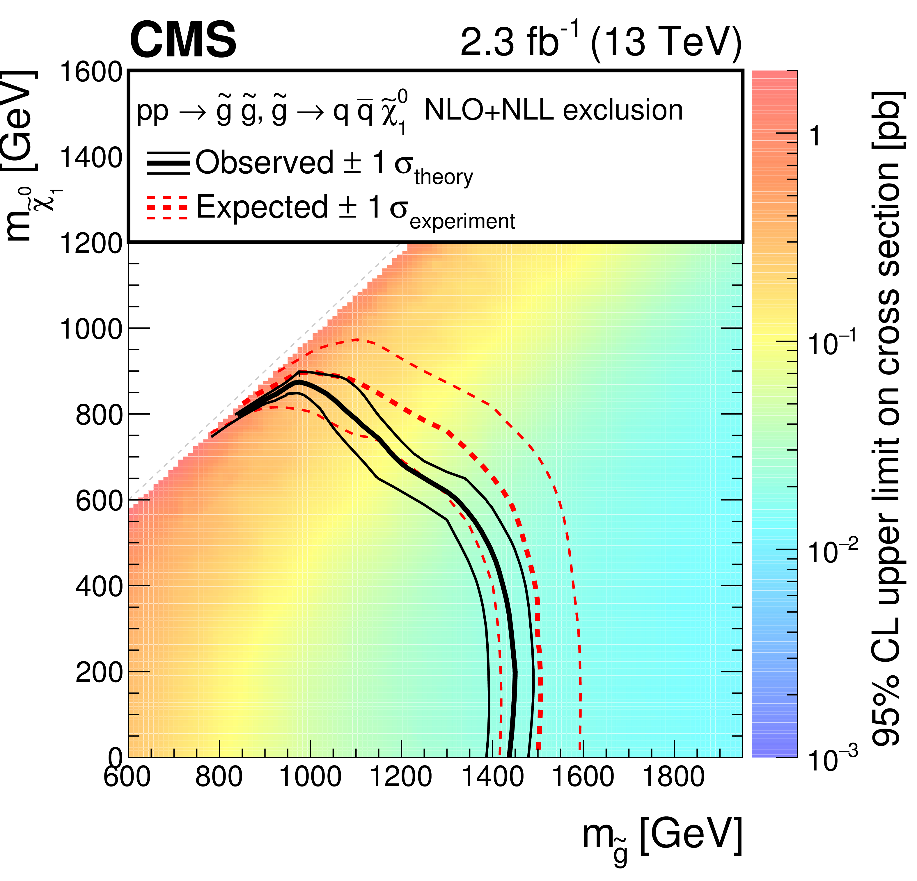
Figure 8-c:
The 95% CL upper limits on the production cross sections for the (a) T1bbbb, (b) T1tttt, (c) T1qqqq, and (d) T5qqqqVV simplified models of supersymmetry, shown as a function of the gluino and LSP masses $ {m_{\tilde{g} }} $ and $ {m_{{\tilde{\chi}^0 }_1}} $. For the T5qqqqVV model, the masses of the intermediate $\tilde{\chi}^0_2$ and $\tilde{\chi}^{\pm} _1$ states are taken to be the mean of $ {m_{{\tilde{\chi}^0 }_1}} $ and $ {m_{\tilde{g} }} $. The solid (black) curves show the observed exclusion contours assuming the NLO+NLL cross sections [55-59], with the corresponding $\pm $1standard deviation uncertainties [75]. The dashed (red) curves present the expected limits with $\pm $1 standard deviation experimental uncertainties. The diagonal dashed (grey) lines indicate the kinematic limits of the respective decay. |
png pdf root |
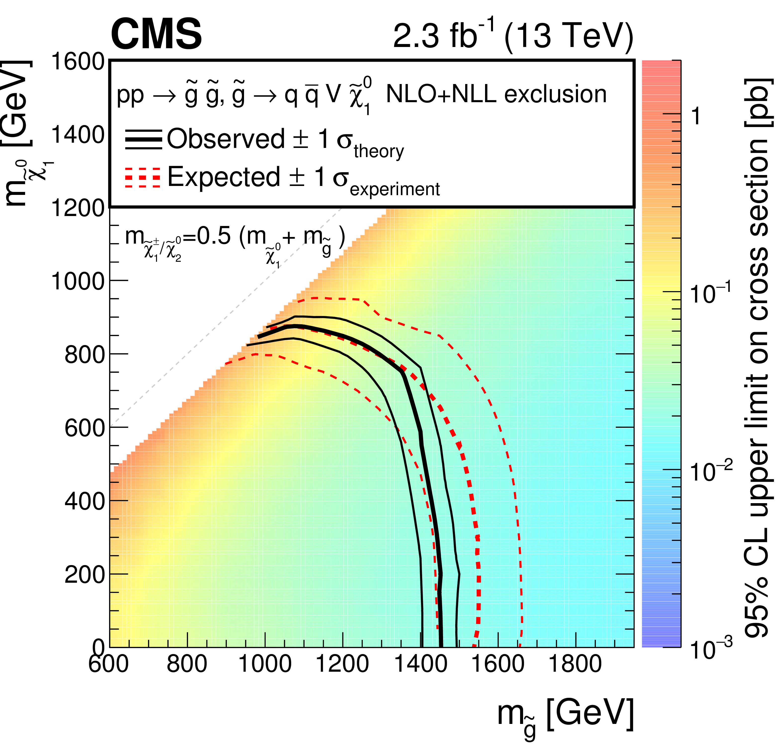
Figure 8-d:
The 95% CL upper limits on the production cross sections for the (a) T1bbbb, (b) T1tttt, (c) T1qqqq, and (d) T5qqqqVV simplified models of supersymmetry, shown as a function of the gluino and LSP masses $ {m_{\tilde{g} }} $ and $ {m_{{\tilde{\chi}^0 }_1}} $. For the T5qqqqVV model, the masses of the intermediate $\tilde{\chi}^0_2$ and $\tilde{\chi}^{\pm} _1$ states are taken to be the mean of $ {m_{{\tilde{\chi}^0 }_1}} $ and $ {m_{\tilde{g} }} $. The solid (black) curves show the observed exclusion contours assuming the NLO+NLL cross sections [55-59], with the corresponding $\pm $1standard deviation uncertainties [75]. The dashed (red) curves present the expected limits with $\pm $1 standard deviation experimental uncertainties. The diagonal dashed (grey) lines indicate the kinematic limits of the respective decay. |
| Tables | |
png pdf |
Table 1:
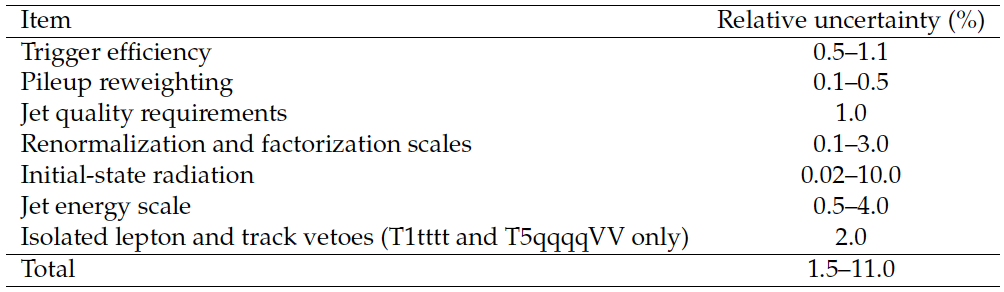
Summary of systematic uncertainties that affect the signal event selection efficiency. The results are averaged over all search regions. The variations correspond to different signal models and choices of the gluino and LSP masses. |
png pdf |
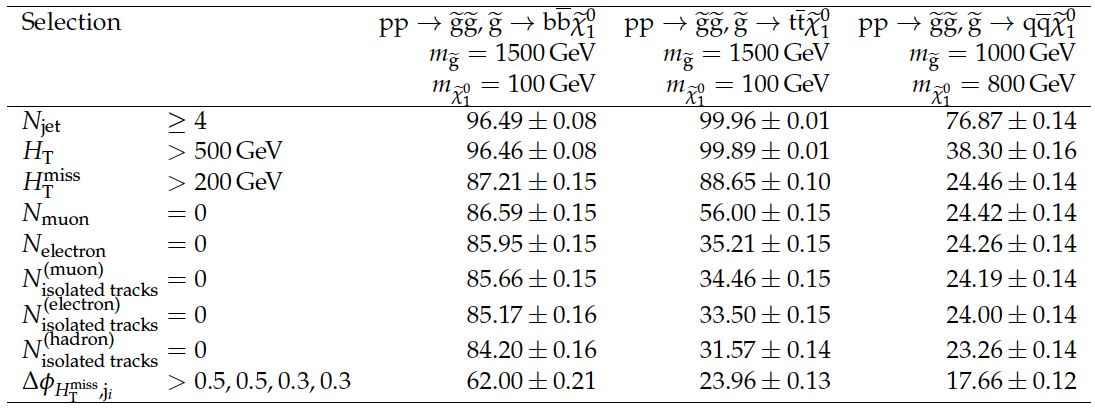
Table 2:
Absolute cumulative efficiencies in % for each step of the event selection process, listed for three representative signal models and choices for the gluino and LSP masses. Only statistical uncertainties are shown. |
png pdf |
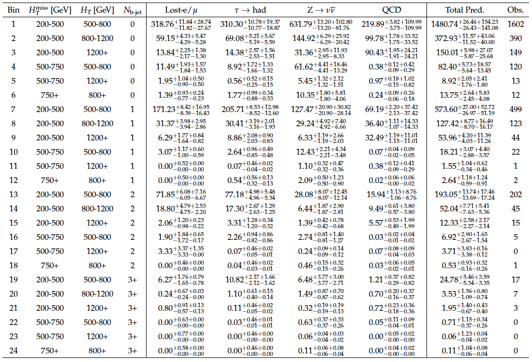
Table 3:
Observed numbers of events and prefit background predictions for $4\leq {N_{\text {jet}}} \leq 6$. These results are displayed in the leftmost section of Fig. 6. The first uncertainty is statistical and the second systematic. |
png pdf |
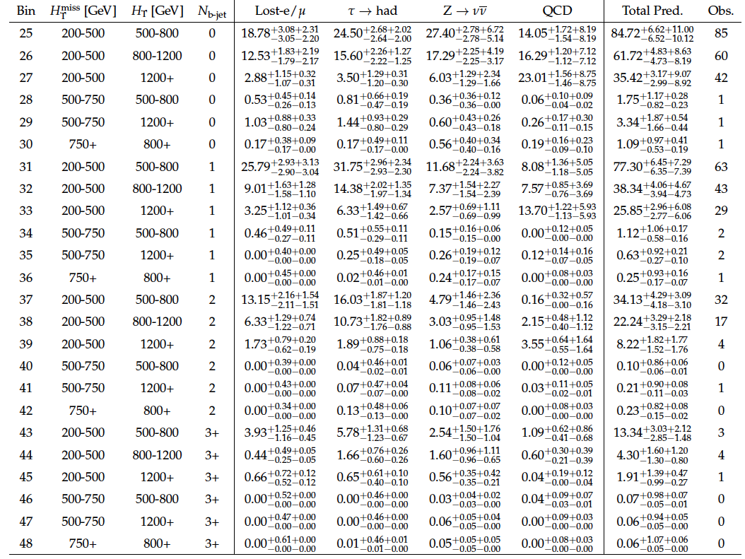
Table 4:
Observed numbers of events and prefit background predictions for $7\leq {N_{\text {jet}}} \leq 8$. These results are displayed in the central section of Fig. 6. The first uncertainty is statistical and the second systematic. |
png pdf |
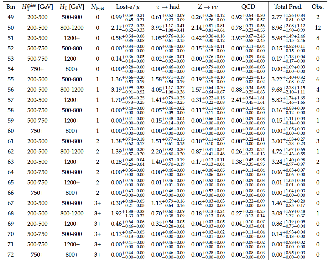
Table 5:
Observed numbers of events and prefit background predictions for $ {N_{\text {jet}}} \geq 9$. These results are displayed in the rightmost section of Fig. 6. The first uncertainty is statistical and the second systematic. |
| Summary |
| A search is presented for an anomalously high rate of events with four or more jets, no identified isolated electron or muon or isolated charged track, large scalar sum $ H_{\mathrm{T}} $ of jet transverse momenta, and large missing transverse momentum, where this latter quantity is measured with the variable $ H_{\mathrm{T}}^{\text{miss}} $, the magnitude of the vector sum of jet transverse momenta. The search is based on a sample of proton-proton collision data collected at $\sqrt{s}=$ 13 TeV with the CMS detector at the CERN LHC in 2015, corresponding to an integrated luminosity of 2.3 fb$^{-1}$. The principal standard model backgrounds, from events with top quarks, W bosons and jets, Z bosons and jets, and QCD multijet production, are evaluated using control samples in the data. The study is performed in the framework of a global likelihood fit in which the observed numbers of events in 72 exclusive bins in a four-dimensional array of $ H_{\mathrm{T}}^{\text{miss}} $, the number of jets, the number of tagged bottom quark jets, and $ H_{\mathrm{T}} $, are compared to the standard model predictions. The standard model background estimates are found to agree with the observed numbers of events within the uncertainties. The results are interpreted with simplified models that, in the context of supersymmetry, correspond to gluino pair production followed by the decay of each gluino to an undetected lightest-supersymmetric-particle (LSP) neutralino $\tilde{\chi}^0_1$ and to a bottom quark-antiquark pair (T1bbbb model), a top quark-antiquark pair (T1tttt model), or a light-flavored quark-antiquark pair (T1qqqq model). We also consider a scenario corresponding to gluino pair production followed by the decay of each gluino to a light-flavored quark-antiquark pair and to either a next-to-lightest neutralino $\tilde{\chi}^0_2$ or a lightest chargino $\tilde{\chi}^{\pm}_1$, with $\tilde{\chi}^0_2\to \mathrm{Z}\tilde{\chi}^0_1$ or $\tilde{\chi}^{\pm}_1\to\mathrm{W}^\pm\tilde{\chi}^0_1$ (T5qqqqVV model). Using the NLO+NLL production cross section as a reference, and for a massless LSP, we exclude gluinos with masses below 1600, 1550, 1440, and 1450 GeV for the four scenarios, respectively, significantly extending the limits from previous searches. |
| Additional Figures | |
png pdf |
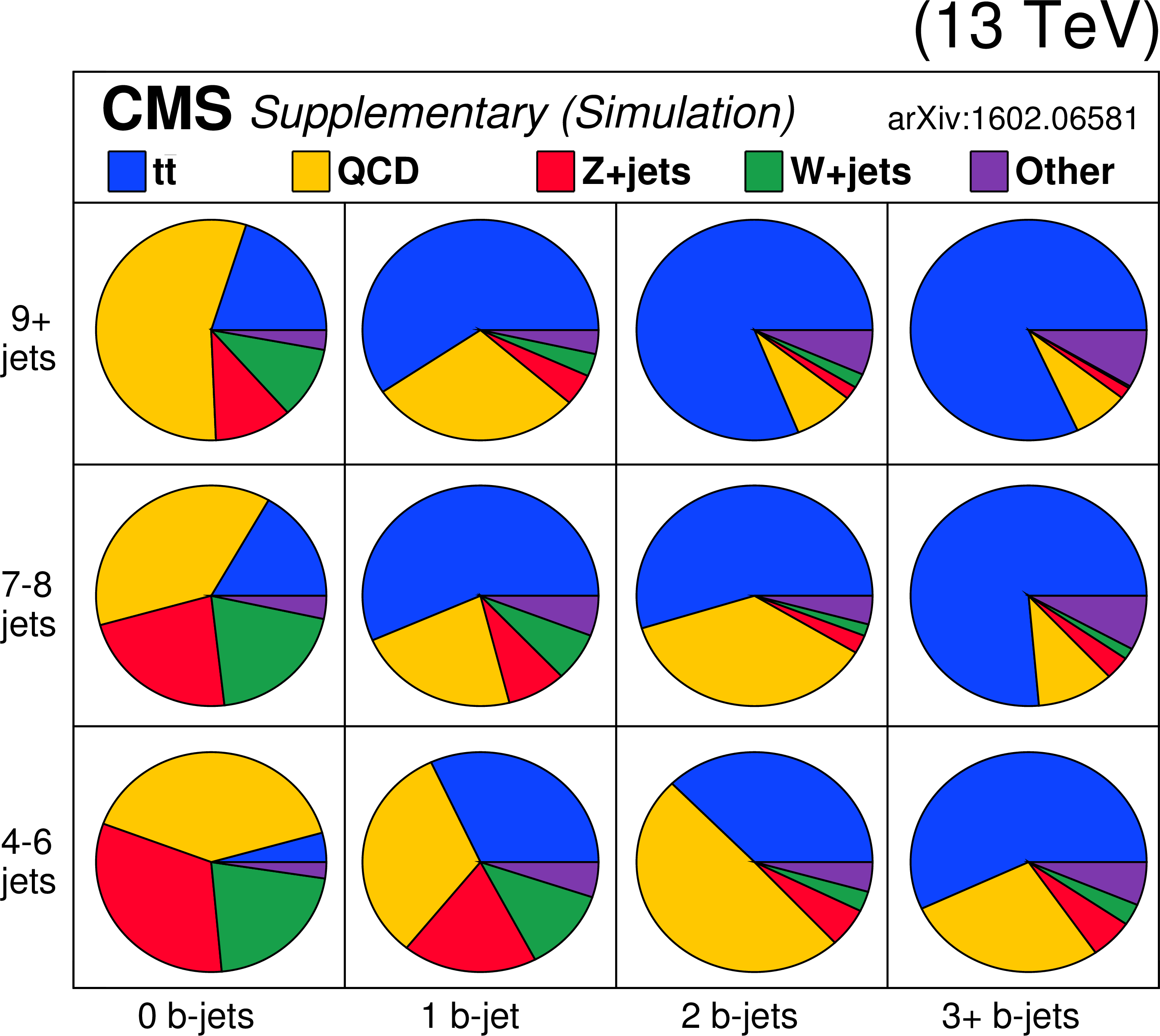
Additional Figure 1:
Background composition in zero-lepton search region ($H_{\mathrm T}^{\mathrm {miss}}> $ 200 GeV, $H_{\mathrm T}> $ 500 GeV) in bins of the number of jets and the number of b-tagged jets. The expected contribution from each process is obtained from simulation after applying the full baseline selection. |
png pdf |
Additional Figure 2-a:
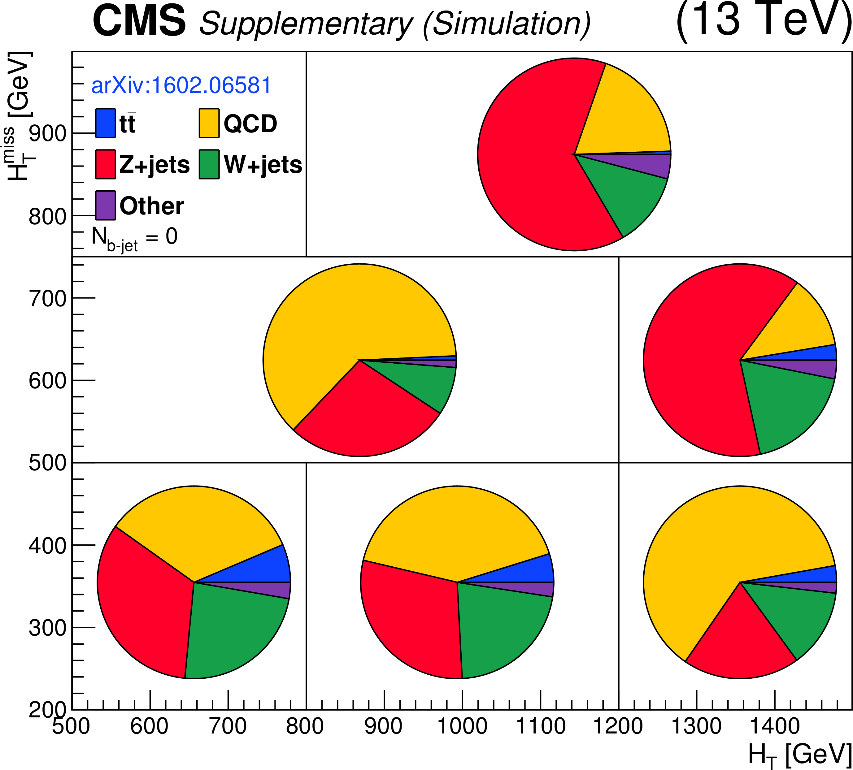
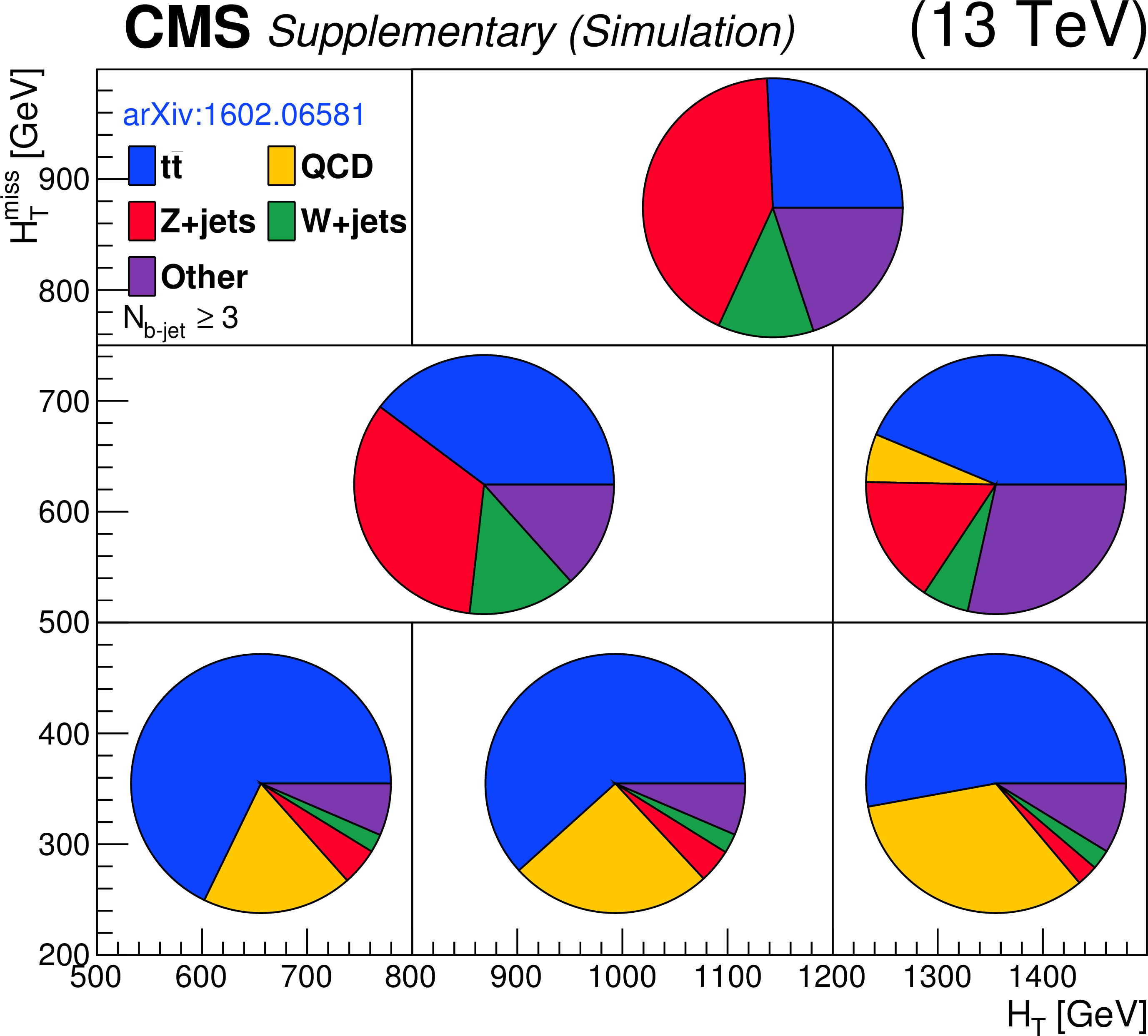
Background composition from simulation in zero-lepton search region in bins of $H_{\mathrm T}^{\mathrm {miss}}$ and $H_{\mathrm T}$. The composition is shown separately for events with 0 b-tagged jets, 1 b-tagged jet, 2 b-tagged jets, and 3 or more b-tagged jets. |
png pdf |
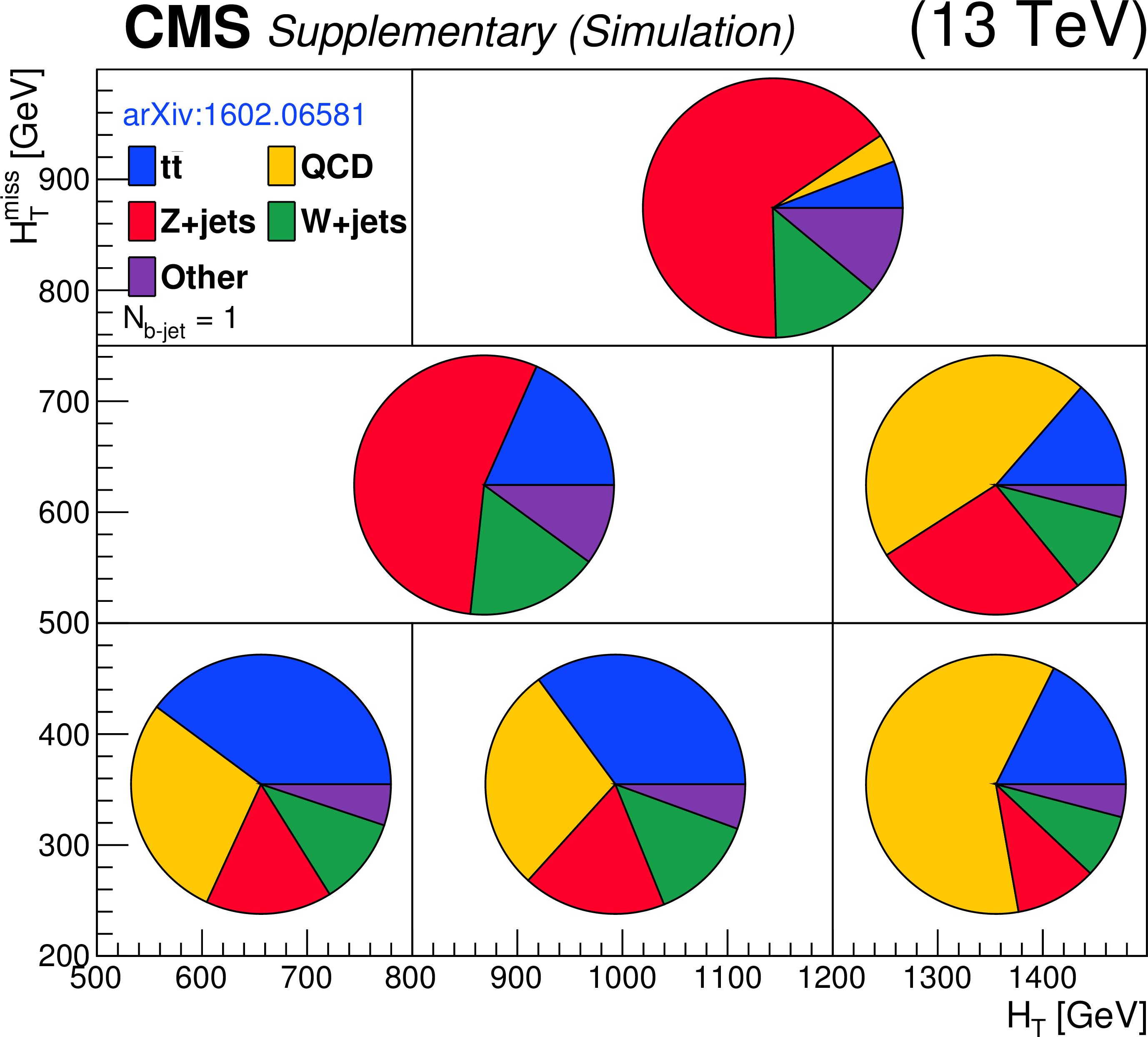
Additional Figure 2-b:
Background composition from simulation in zero-lepton search region in bins of $H_{\mathrm T}^{\mathrm {miss}}$ and $H_{\mathrm T}$. The composition is shown separately for events with 0 b-tagged jets, 1 b-tagged jet, 2 b-tagged jets, and 3 or more b-tagged jets. |
png pdf |
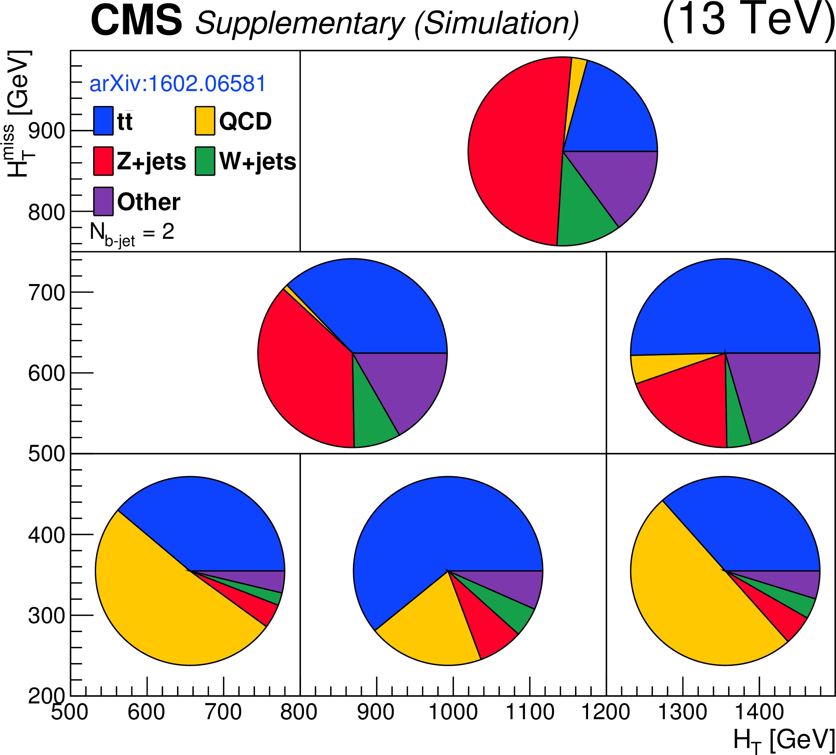
Additional Figure 2-c:
Background composition from simulation in zero-lepton search region in bins of $H_{\mathrm T}^{\mathrm {miss}}$ and $H_{\mathrm T}$. The composition is shown separately for events with 0 b-tagged jets, 1 b-tagged jet, 2 b-tagged jets, and 3 or more b-tagged jets. |
png pdf |
Additional Figure 2-d:
Background composition from simulation in zero-lepton search region in bins of $H_{\mathrm T}^{\mathrm {miss}}$ and $H_{\mathrm T}$. The composition is shown separately for events with 0 b-tagged jets, 1 b-tagged jet, 2 b-tagged jets, and 3 or more b-tagged jets. |
png pdf |
Additional Figure 3-a:
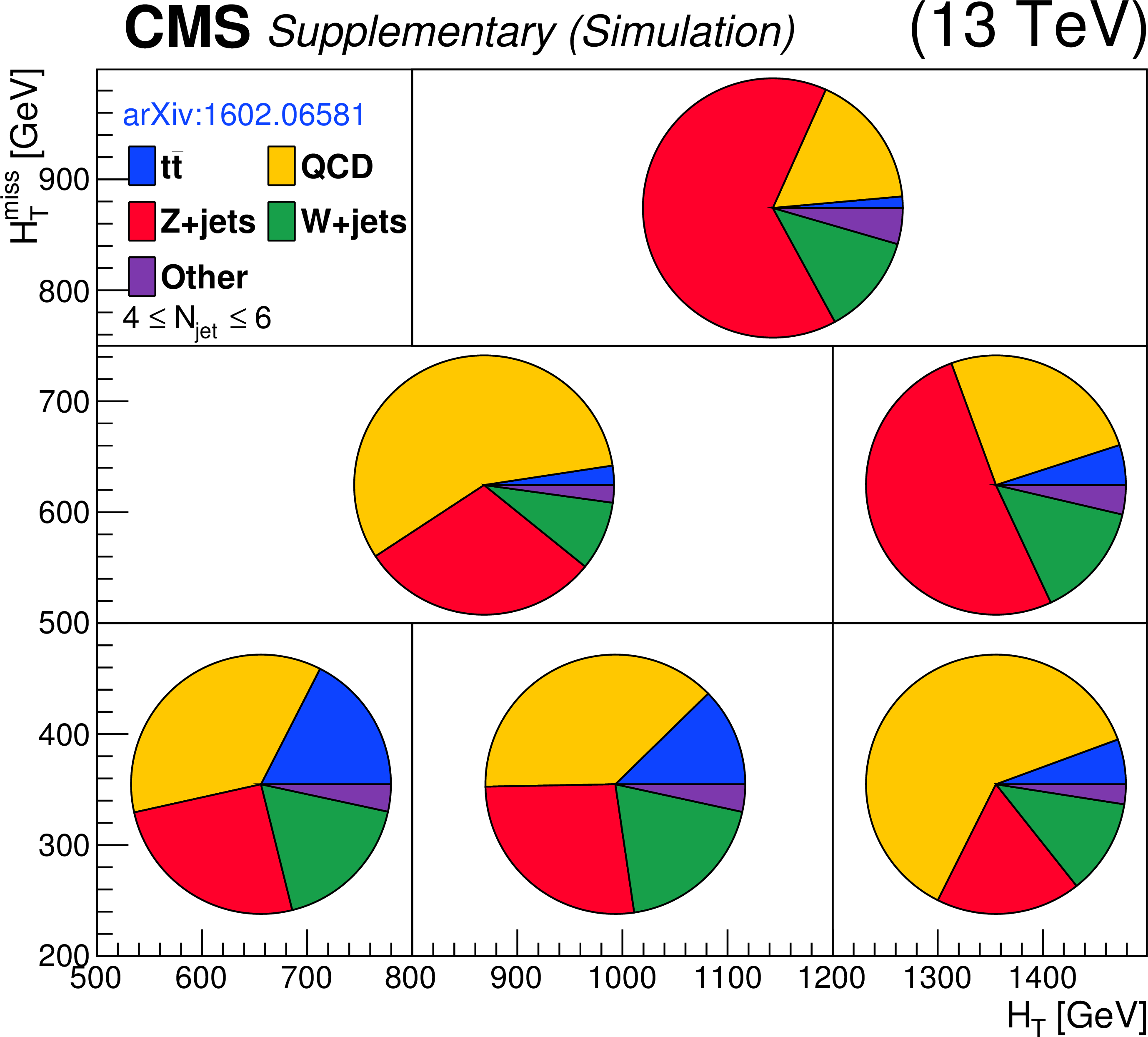
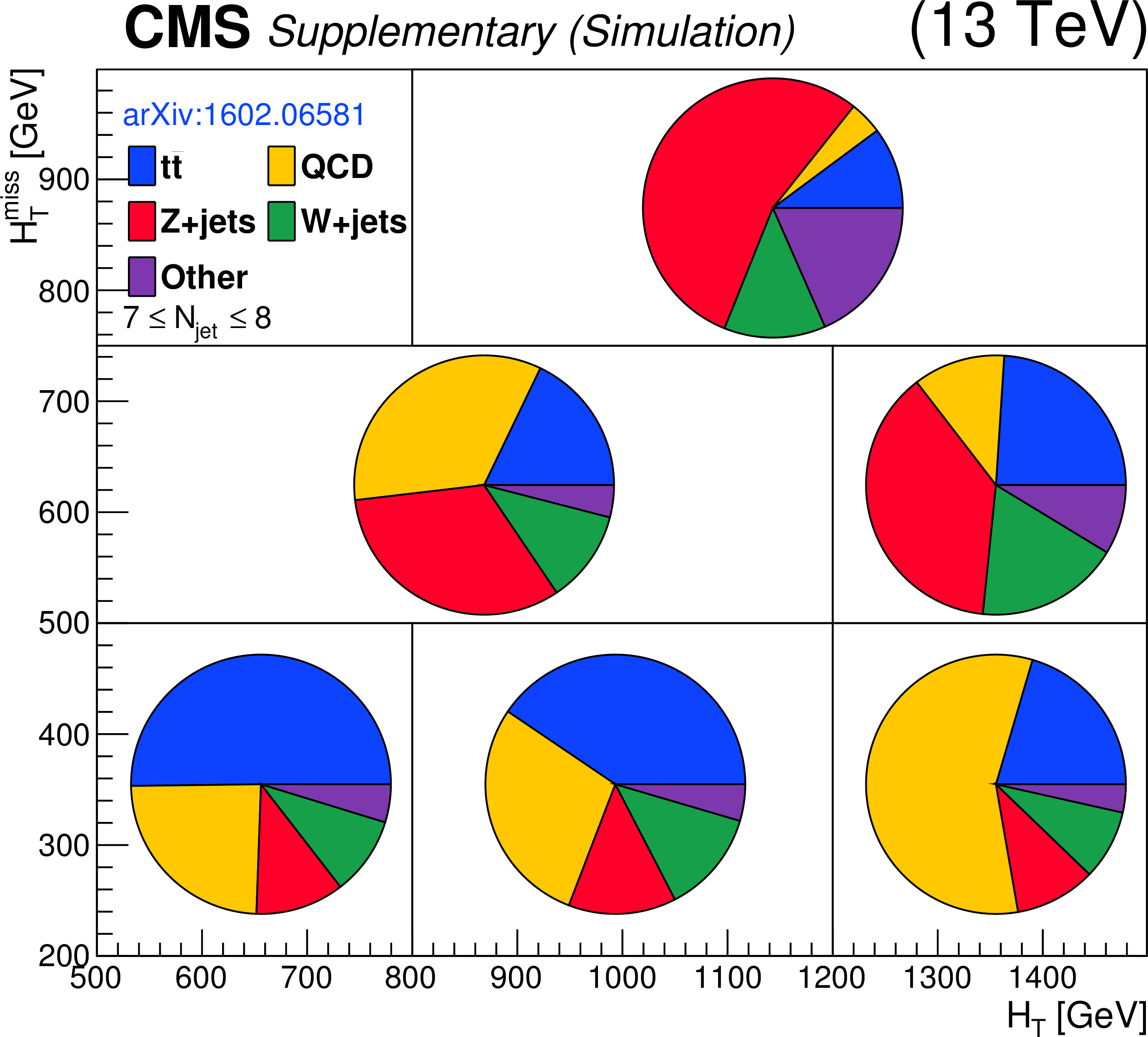
Background composition from simulation in zero-lepton search region in bins of $H_{\mathrm T}^{\mathrm {miss}}$ and $H_{\mathrm T}$. The composition is shown separately for events with 4-6 jets, 7-8 jets, and 9 or more jets. |
png pdf |
Additional Figure 3-b:
Background composition from simulation in zero-lepton search region in bins of $H_{\mathrm T}^{\mathrm {miss}}$ and $H_{\mathrm T}$. The composition is shown separately for events with 4-6 jets, 7-8 jets, and 9 or more jets. |
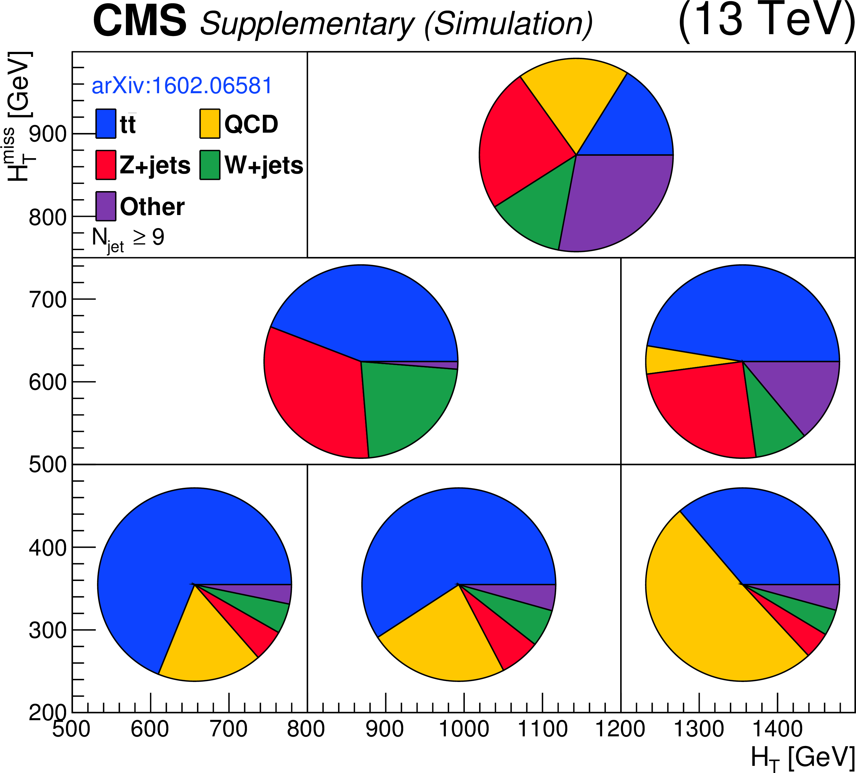
png pdf |
Additional Figure 3-c:
Background composition from simulation in zero-lepton search region in bins of $H_{\mathrm T}^{\mathrm {miss}}$ and $H_{\mathrm T}$. The composition is shown separately for events with 4-6 jets, 7-8 jets, and 9 or more jets. |

png pdf |
Additional Figure 4-a:
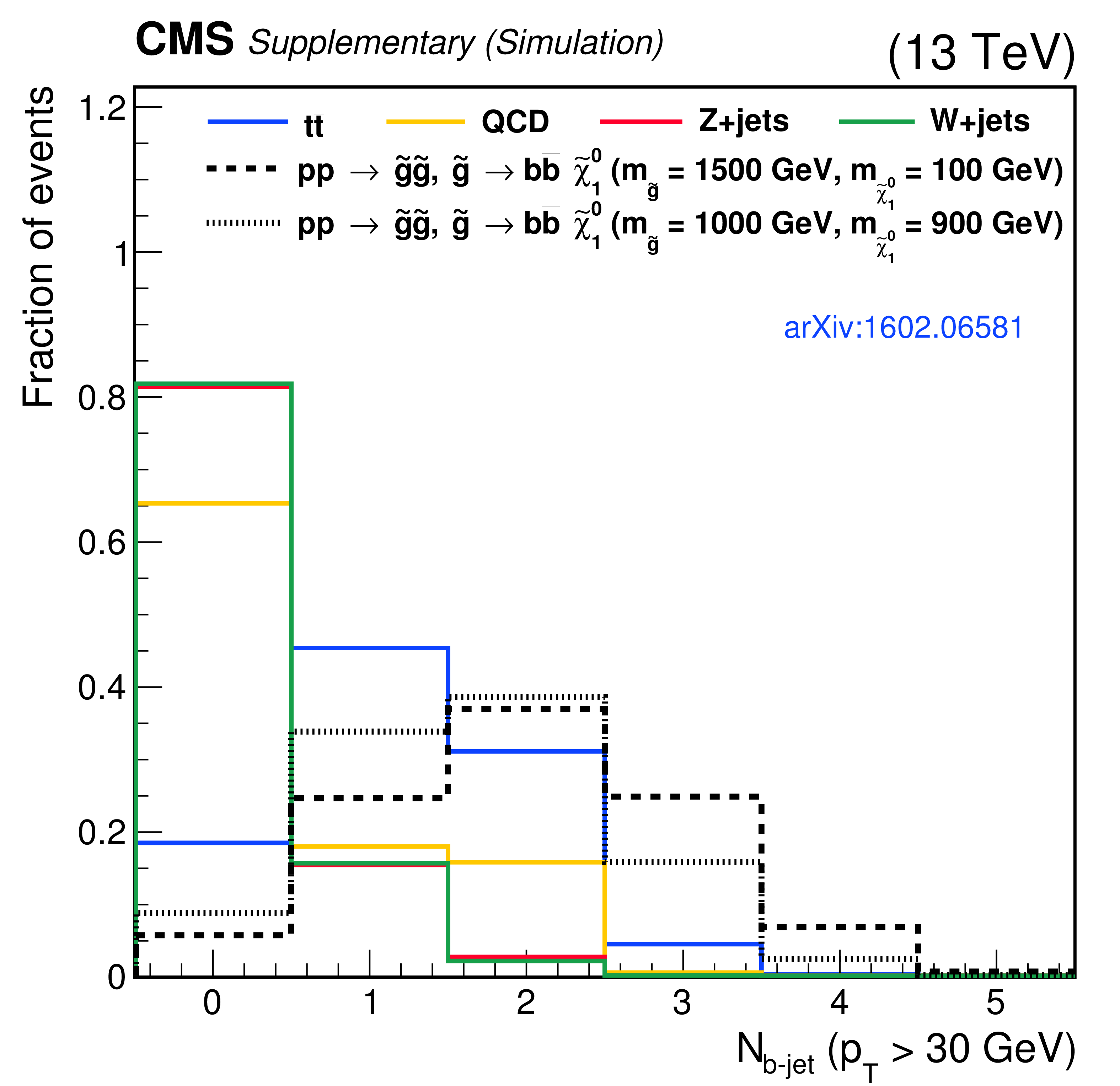
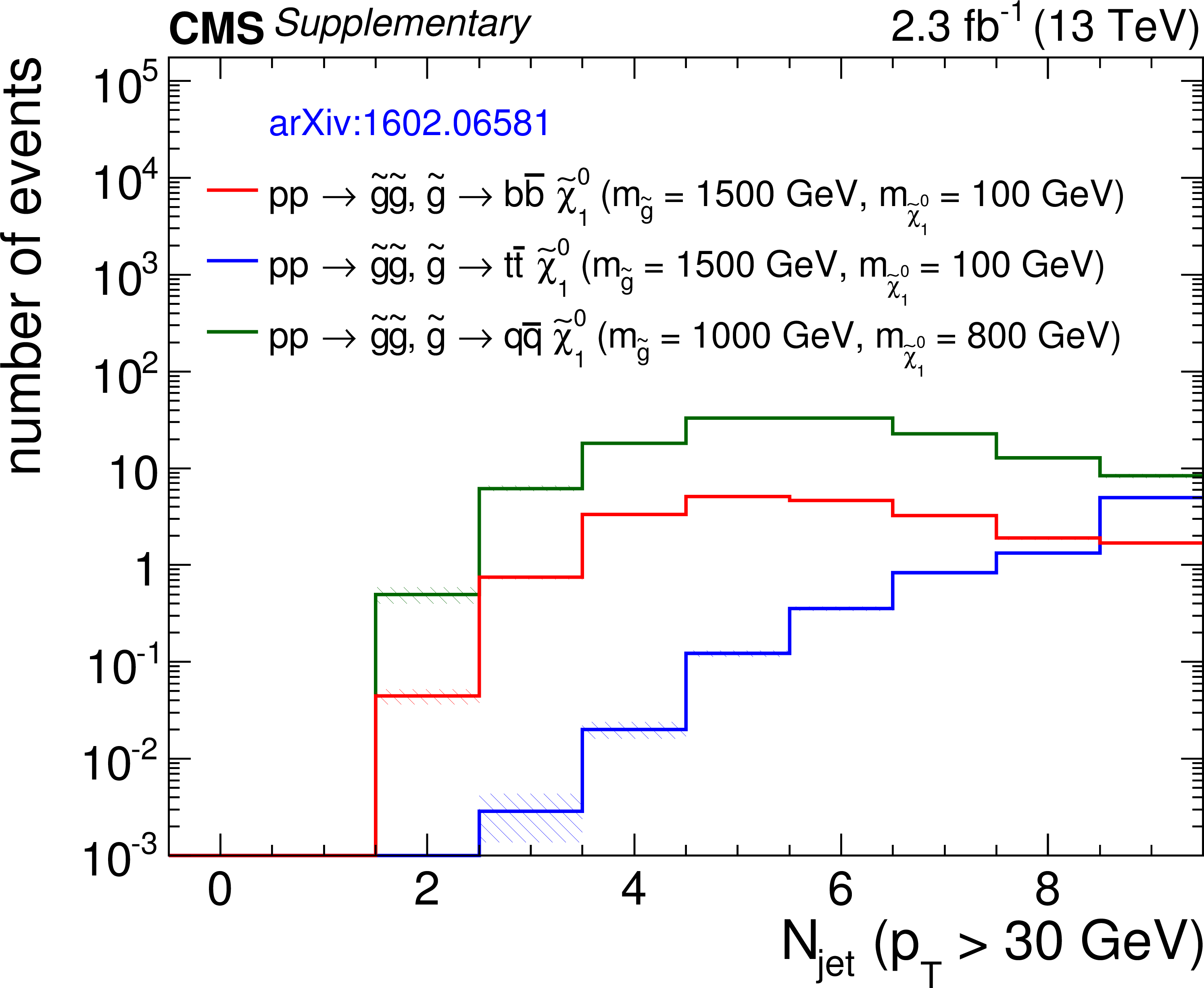
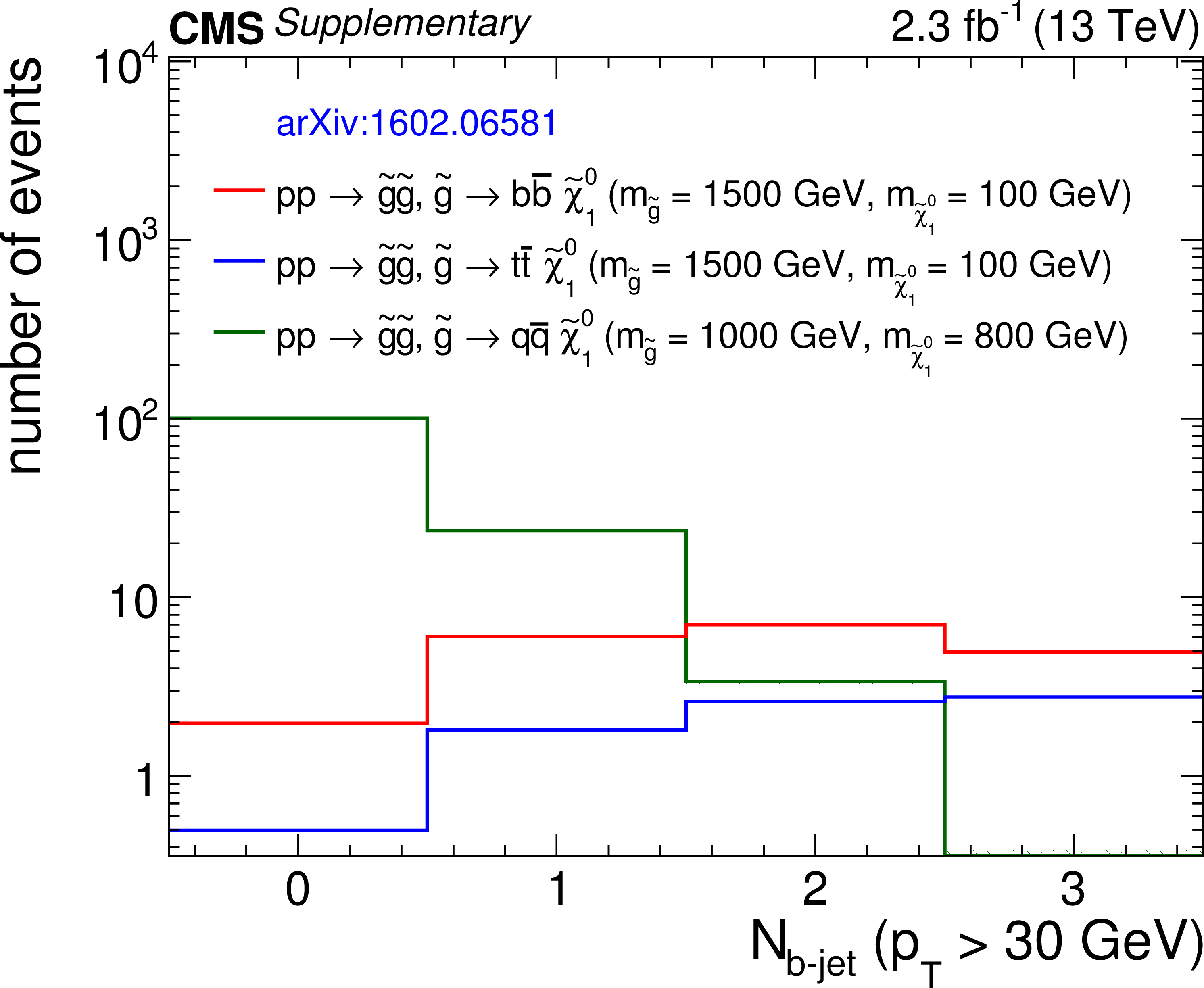
Kinematic shape comparisons showing distributions of $H_{\mathrm T}$, $H_{\mathrm T}^{\mathrm miss}$, the number of b-tagged jets, and the number of jets for the main background processes and six example gluino production signal models. The full baseline selection is applied in each plot. |

png pdf |
Additional Figure 4-b:
Kinematic shape comparisons showing distributions of $H_{\mathrm T}$, $H_{\mathrm T}^{\mathrm miss}$, the number of b-tagged jets, and the number of jets for the main background processes and six example gluino production signal models. The full baseline selection is applied in each plot. |

png pdf |
Additional Figure 4-c:
Kinematic shape comparisons showing distributions of $H_{\mathrm T}$, $H_{\mathrm T}^{\mathrm miss}$, the number of b-tagged jets, and the number of jets for the main background processes and six example gluino production signal models. The full baseline selection is applied in each plot. |
png pdf |
Additional Figure 4-d:
Kinematic shape comparisons showing distributions of $H_{\mathrm T}$, $H_{\mathrm T}^{\mathrm miss}$, the number of b-tagged jets, and the number of jets for the main background processes and six example gluino production signal models. The full baseline selection is applied in each plot. |
png pdf |
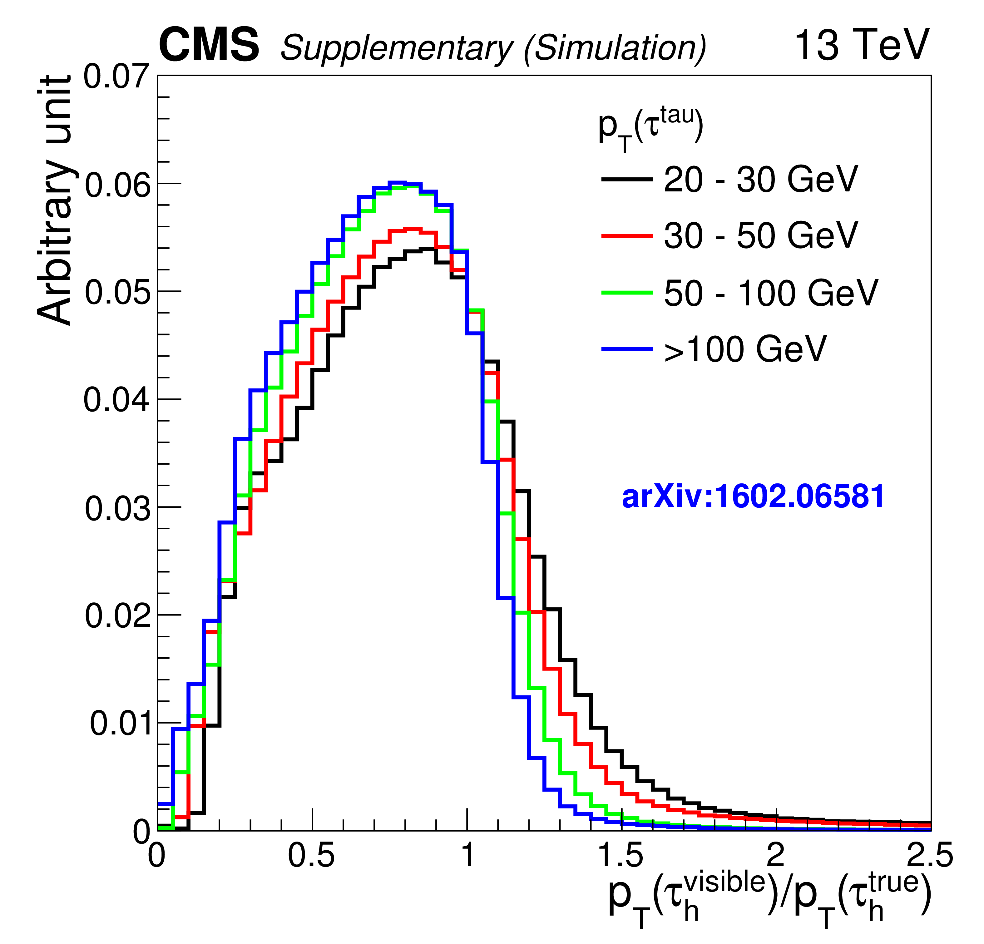
Additional Figure 5:
The hadronically-decaying $\tau $ lepton ($\tau _{h}$) response templates: distributions of $\tau _\mathrm {h}$ visible-$p_\mathrm {T}$ over true $p_\mathrm {T}$ of $\tau _\mathrm {h}$, $p_{\mathrm T}(\tau _{\mathrm h}^\mathrm {visible})/p_{\mathrm T}(\tau _{\mathrm h}^\mathrm {true})$, in intervals of $p_{\mathrm T}(\tau _{\mathrm h}^\mathrm {true})$ as determined from simulated $\mathrm{ t \bar{t} }$ and W+jets events. |
png pdf |
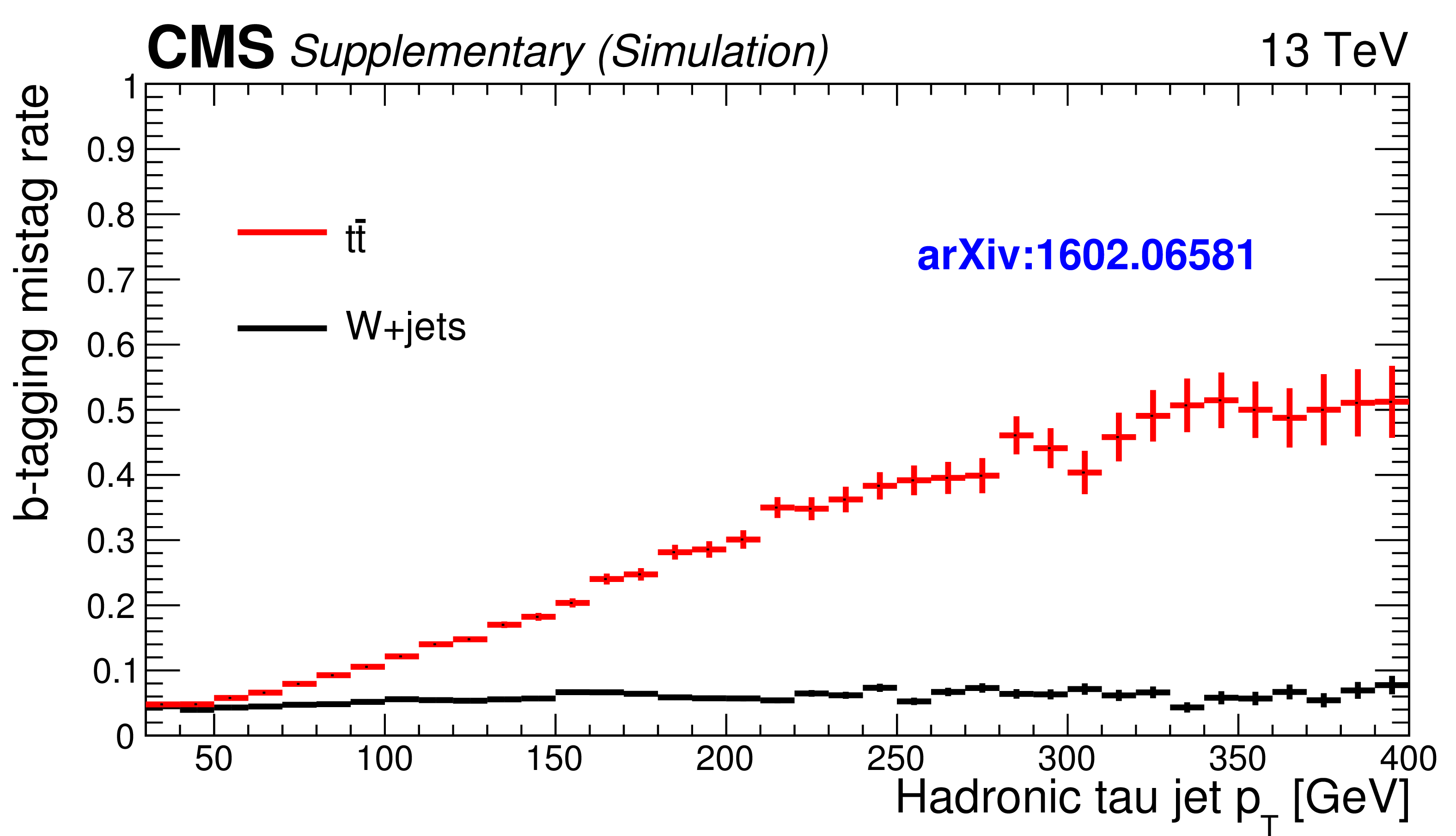
Additional Figure 6:
The b-tagging mistag rate of $\tau _{h}$ jets as function of transverse momentum in simulated $\mathrm{ t \bar{t} }$ and W+jets events. The rise of the tagging rate at high $p_\mathrm {T}$ in $\mathrm{ t \bar{t} }$ events is due to the proximity of b-quarks from the same top quark decays. |
png pdf |
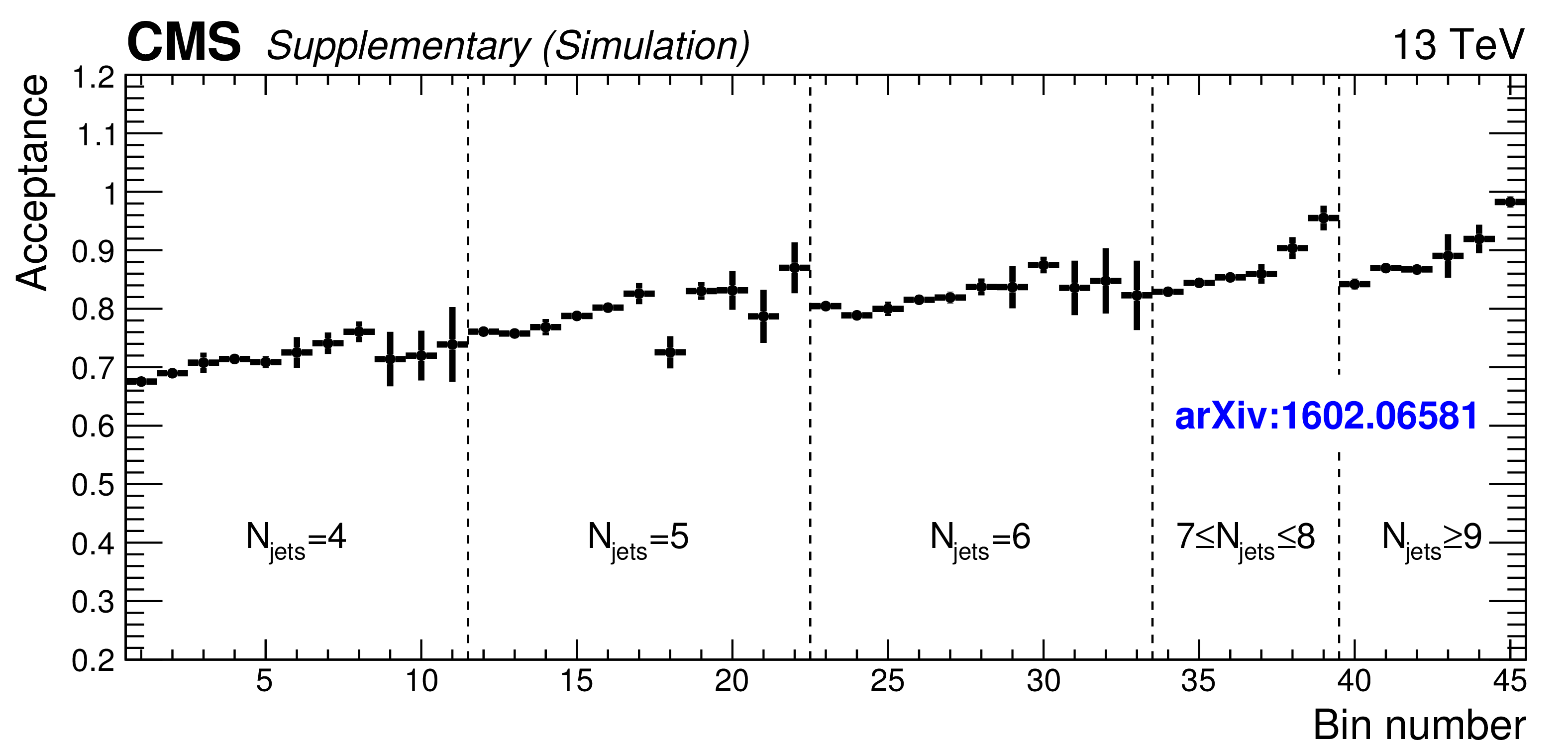
Additional Figure 7:
Acceptance $\epsilon ^{\mu }_{Acc}$ of hadronically-decaying $\tau $ leptons for $p_{\mathrm T}> $ 20 GeV and $|\eta |< $ 2.1 . The results are shown as a function of $H_{\mathrm T}^{\mathrm miss}$, $H_{\mathrm T}$, and $N_{\mathrm jet}$, integrated over the four bins of $N_{\mathrm b-jet}$ (in total 45 bins). |
png pdf |
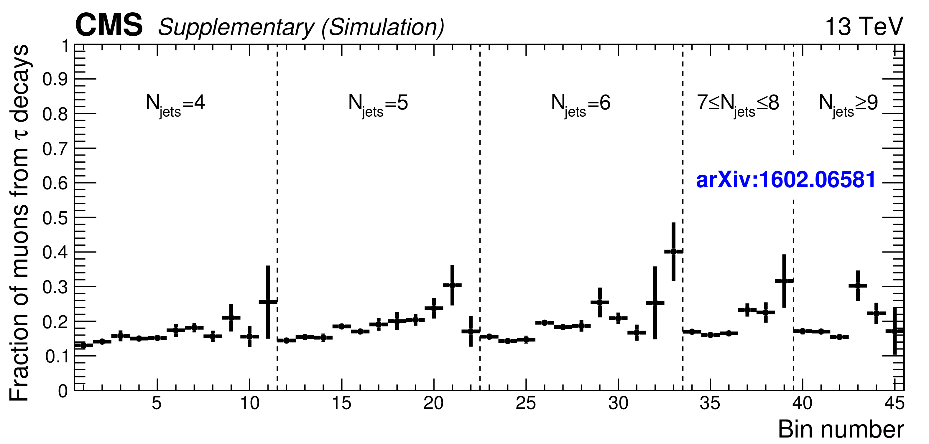
Additional Figure 8:
The fraction $f$ of muons from $\tau $ decays in the single-muon control sample, as determined from simulation. The results are shown as a function of $H_{\mathrm T}^{\mathrm miss}$, $H_{\mathrm T}$, and $N_{\mathrm jet}$, integrated over the four bins of $N_{\mathrm b-jet}$ (in total 45 bins). |

png pdf |
Additional Figure 9:
The efficiency $\epsilon _{m_{T}}$ of the muon $m_{T}$ selection. The results are shown as a function of $H_{\mathrm T}^{\mathrm miss}$, $H_{\mathrm T}$, and $N_{\mathrm jet}$, integrated over the four bins of $N_{\mathrm b-jet}$ (in total 45 bins). |

png pdf |
Additional Figure 10:
The isolated-track veto efficiency $\epsilon _{isotrk}$. The results are shown as a function of $H_{\mathrm T}^{\mathrm miss}$, $H_{\mathrm T}$, and $N_{\mathrm jet}$, integrated over the four bins of $N_{\mathrm b-jet}$ (in total 45 bins). |
png pdf |
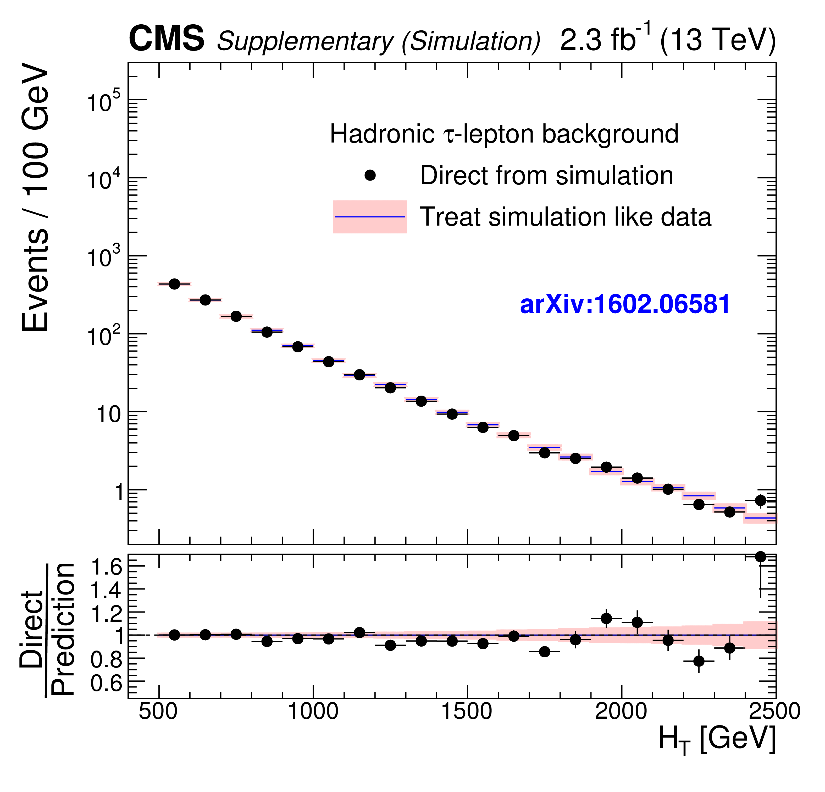
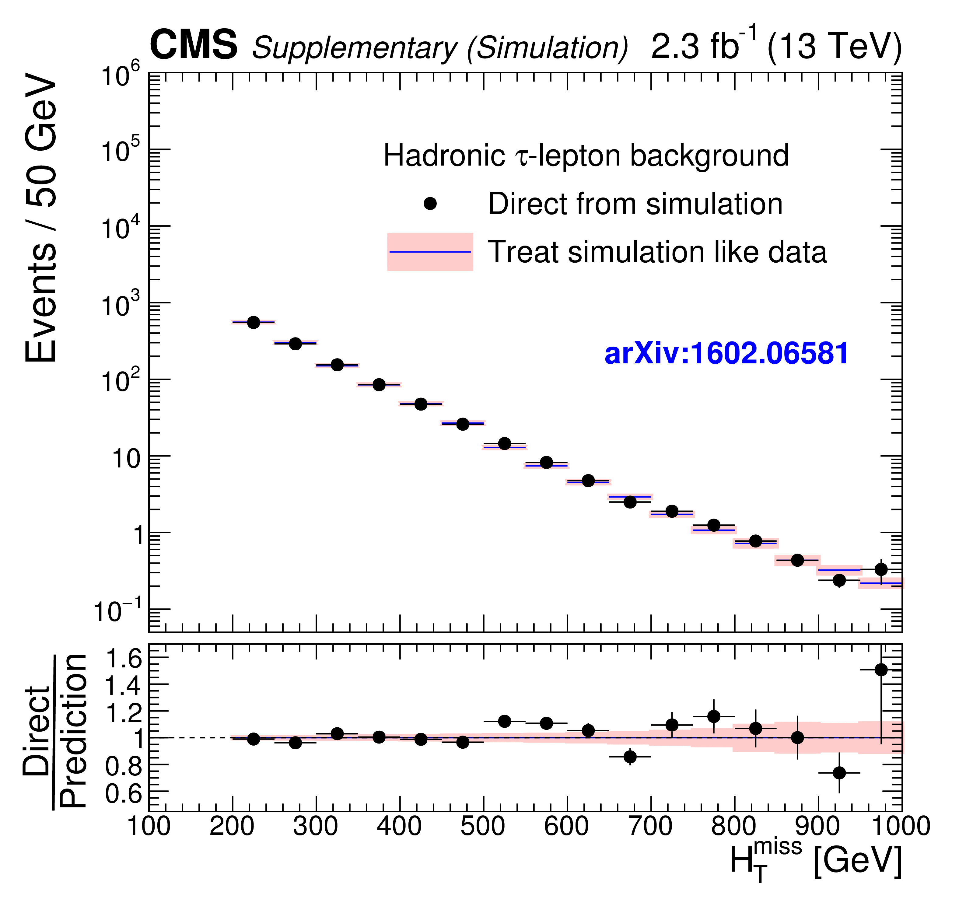
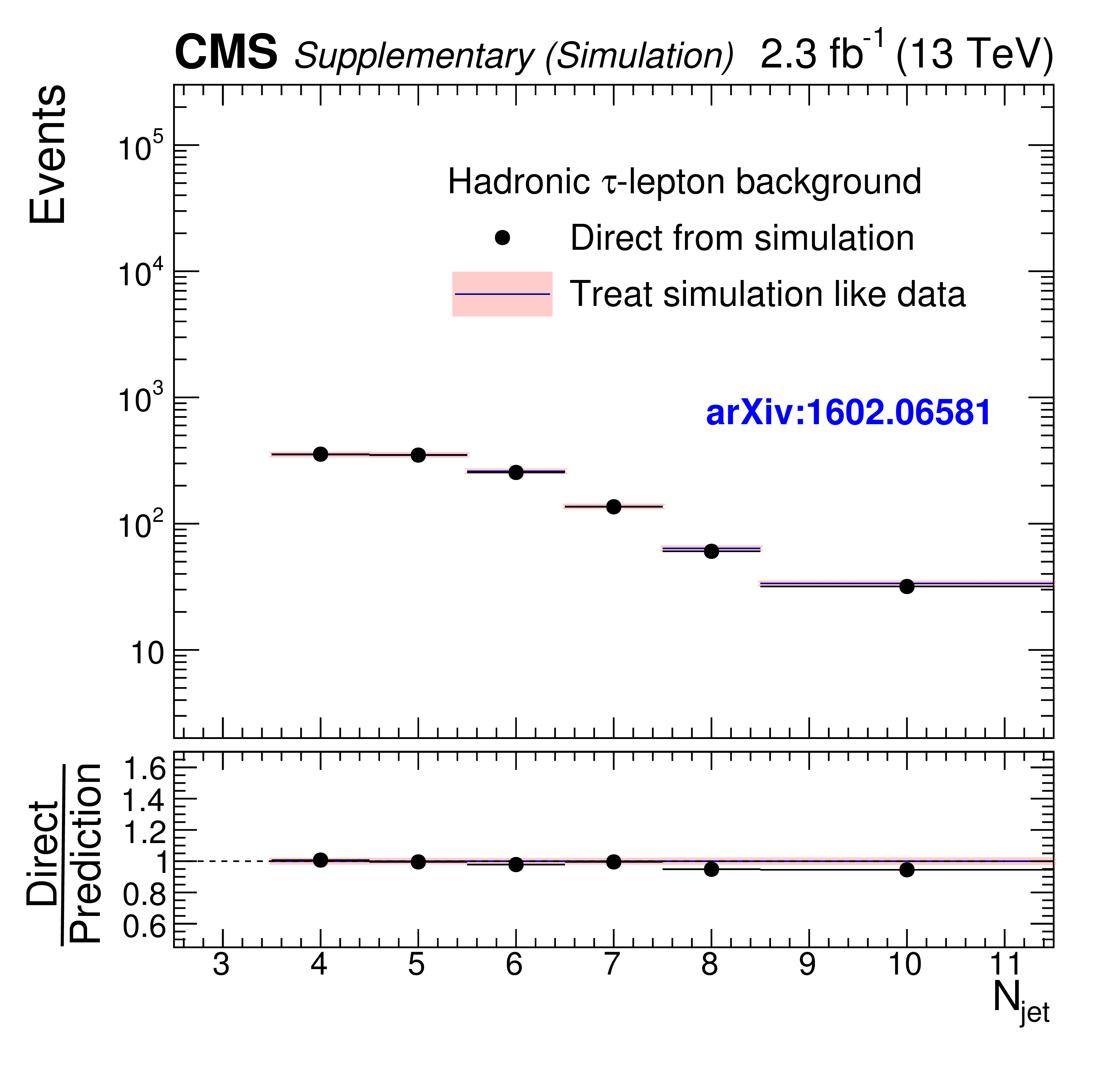
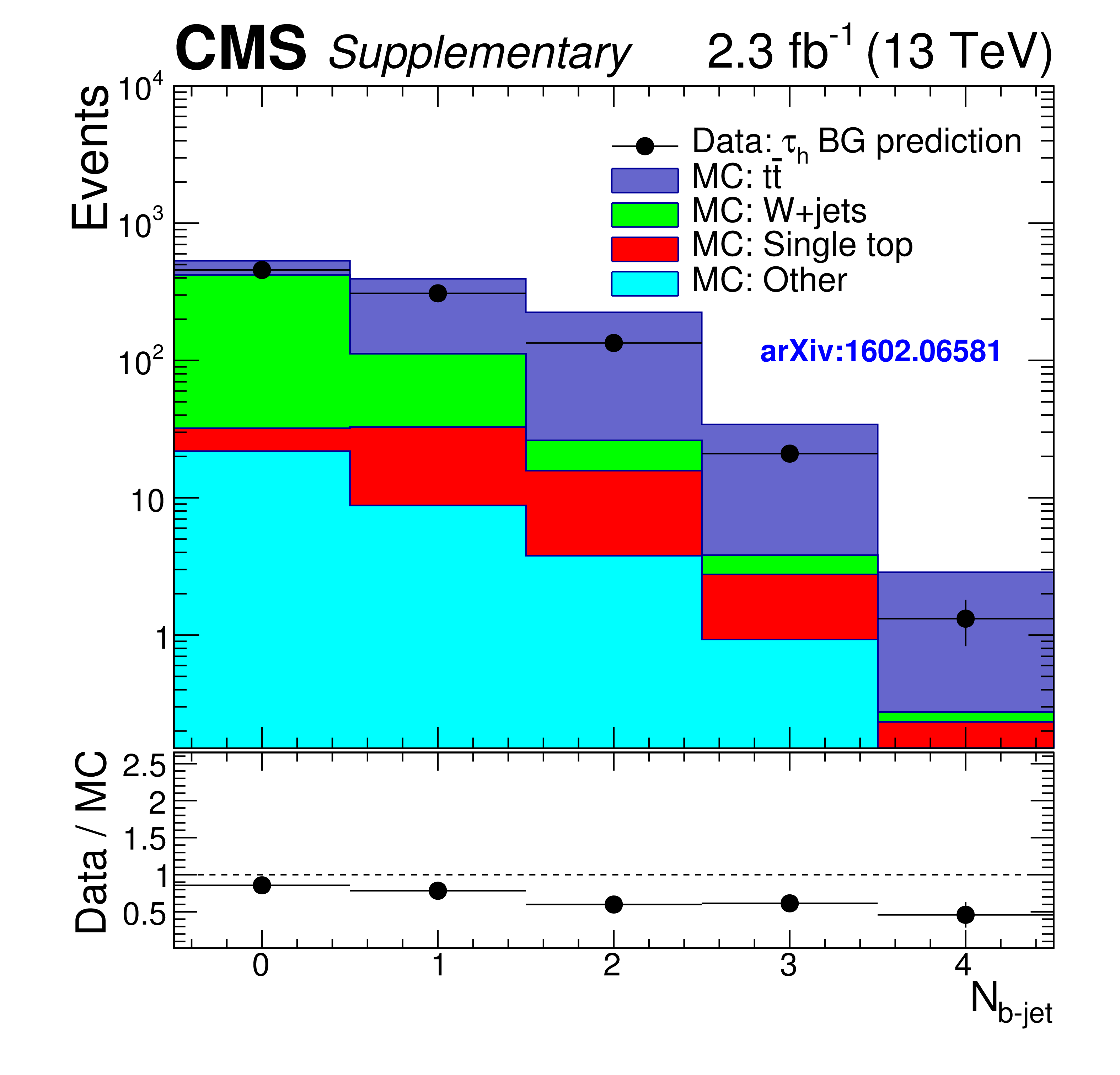
Additional Figure 11-a:
Distributions of $H_{\mathrm T}$, $H_{\mathrm T}^{\mathrm miss}$, the number of b-tagged jets, and the number of jets in $\tau _{h}$ background events as predicted directly from simulation (solid points) and as predicted by the data-driven background-determination procedure (shaded regions), for the baseline selection. The simulation simulation includes $\mathrm{ t \bar{t} }$, W+jets, single top quark, and other rare SM process events. |
png pdf |
Additional Figure 11-b:
Distributions of $H_{\mathrm T}$, $H_{\mathrm T}^{\mathrm miss}$, the number of b-tagged jets, and the number of jets in $\tau _{h}$ background events as predicted directly from simulation (solid points) and as predicted by the data-driven background-determination procedure (shaded regions), for the baseline selection. The simulation simulation includes $\mathrm{ t \bar{t} }$, W+jets, single top quark, and other rare SM process events. |
png pdf |
Additional Figure 11-c:
Distributions of $H_{\mathrm T}$, $H_{\mathrm T}^{\mathrm miss}$, the number of b-tagged jets, and the number of jets in $\tau _{h}$ background events as predicted directly from simulation (solid points) and as predicted by the data-driven background-determination procedure (shaded regions), for the baseline selection. The simulation simulation includes $\mathrm{ t \bar{t} }$, W+jets, single top quark, and other rare SM process events. |
png pdf |
Additional Figure 11-d:
Distributions of $H_{\mathrm T}$, $H_{\mathrm T}^{\mathrm miss}$, the number of b-tagged jets, and the number of jets in $\tau _{h}$ background events as predicted directly from simulation (solid points) and as predicted by the data-driven background-determination procedure (shaded regions), for the baseline selection. The simulation simulation includes $\mathrm{ t \bar{t} }$, W+jets, single top quark, and other rare SM process events. |
png pdf |
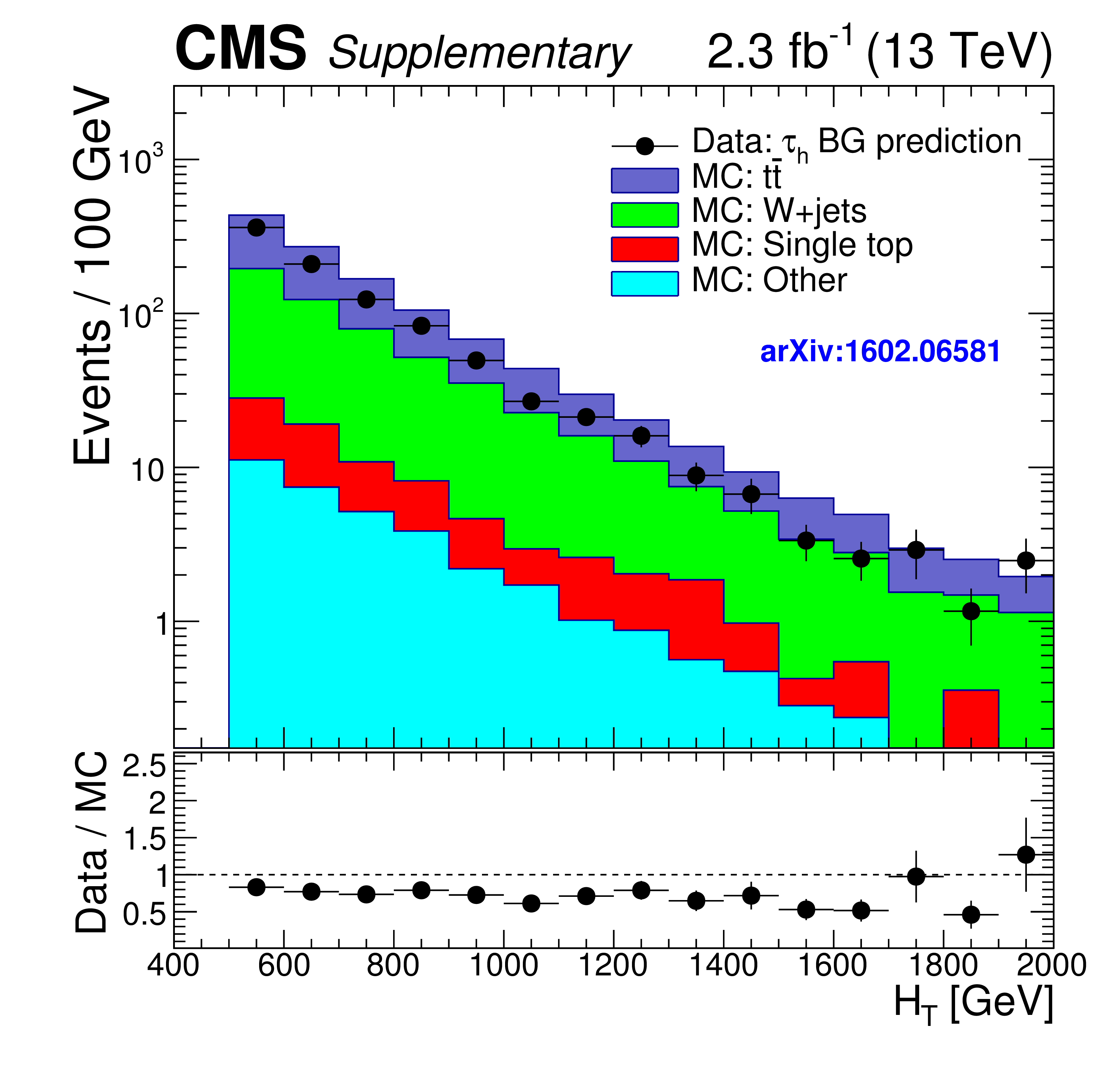
Additional Figure 12-a:
Distributions of $H_{\mathrm T}$, $H_{\mathrm T}^{\mathrm miss}$, the number of b-tagged jets, and the number of jets in $\tau _{h}$ background events as predicted by performing the data driven background-determination procedure on the 2.3 fb$^{-1}$ of data (shaded regions), compared to the $\tau _{h}$ background expectation from simulation (solid points) for the baseline selection. The simulation includes $\mathrm{ t \bar{t} }$, W+jets, single top quark, and other rare SM process events. |
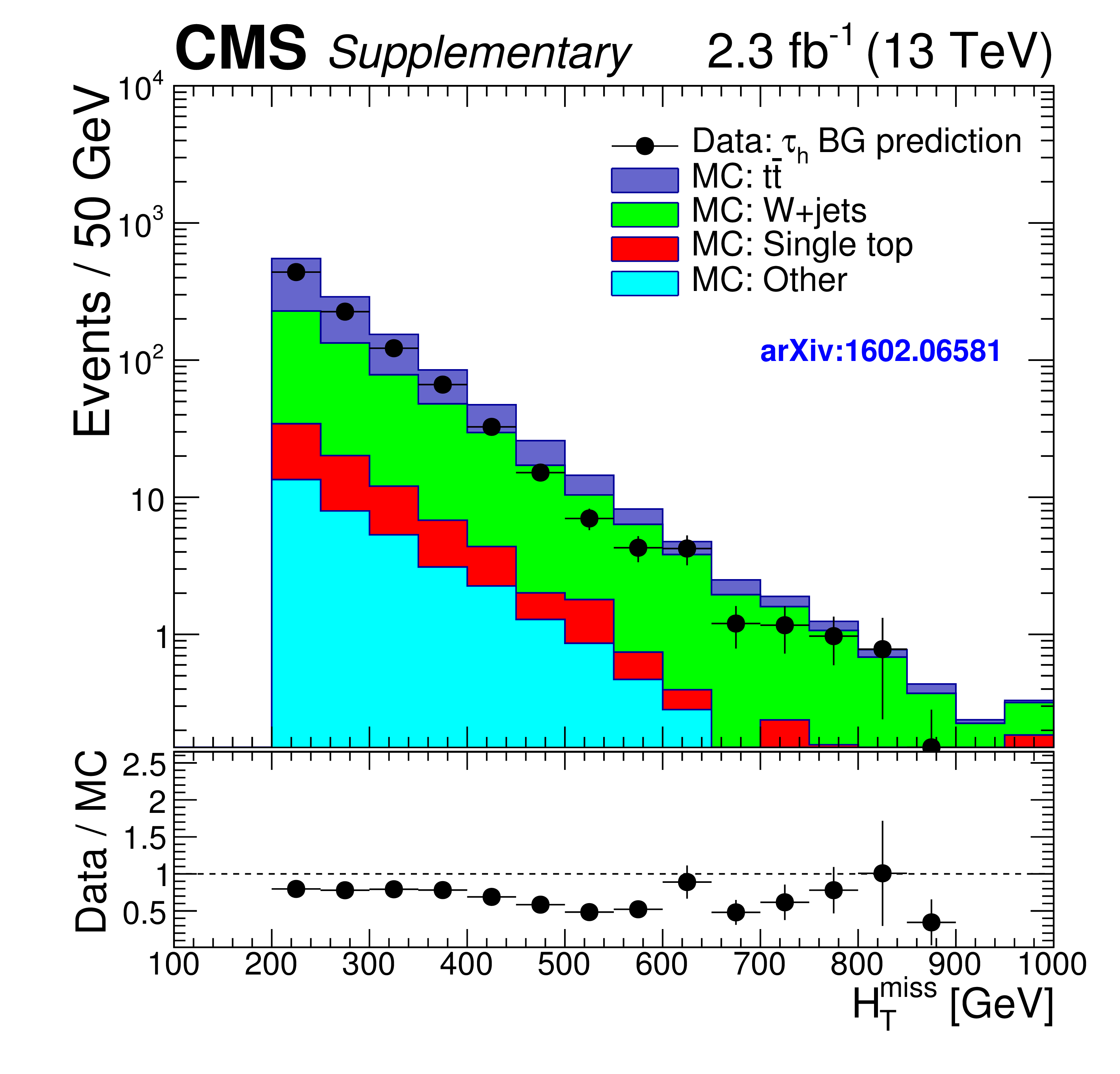
png pdf |
Additional Figure 12-b:
Distributions of $H_{\mathrm T}$, $H_{\mathrm T}^{\mathrm miss}$, the number of b-tagged jets, and the number of jets in $\tau _{h}$ background events as predicted by performing the data driven background-determination procedure on the 2.3 fb$^{-1}$ of data (shaded regions), compared to the $\tau _{h}$ background expectation from simulation (solid points) for the baseline selection. The simulation includes $\mathrm{ t \bar{t} }$, W+jets, single top quark, and other rare SM process events. |
png pdf |
Additional Figure 12-c:
Distributions of $H_{\mathrm T}$, $H_{\mathrm T}^{\mathrm miss}$, the number of b-tagged jets, and the number of jets in $\tau _{h}$ background events as predicted by performing the data driven background-determination procedure on the 2.3 fb$^{-1}$ of data (shaded regions), compared to the $\tau _{h}$ background expectation from simulation (solid points) for the baseline selection. The simulation includes $\mathrm{ t \bar{t} }$, W+jets, single top quark, and other rare SM process events. |
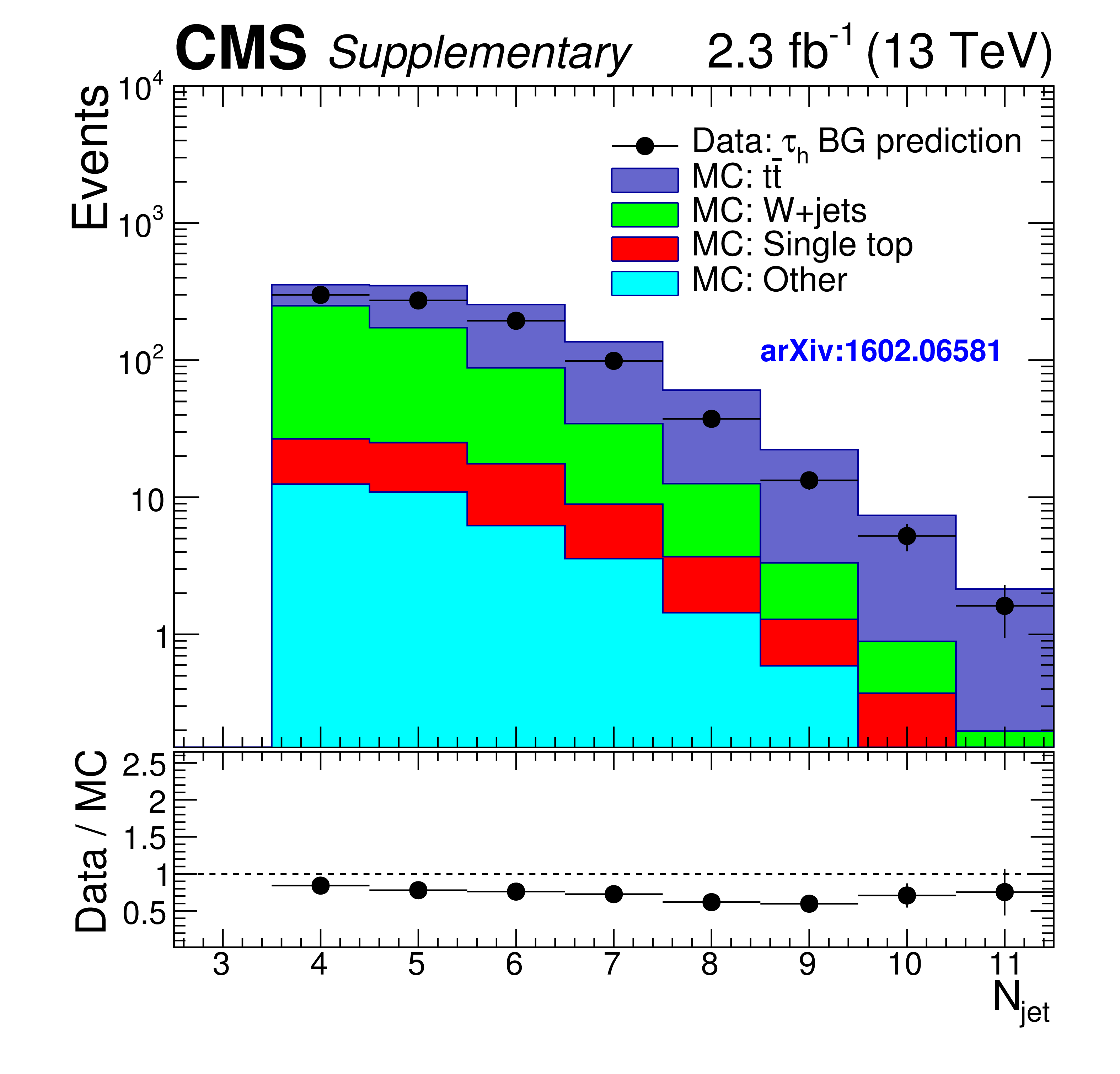
png pdf |
Additional Figure 12-d:
Distributions of $H_{\mathrm T}$, $H_{\mathrm T}^{\mathrm miss}$, the number of b-tagged jets, and the number of jets in $\tau _{h}$ background events as predicted by performing the data driven background-determination procedure on the 2.3 fb$^{-1}$ of data (shaded regions), compared to the $\tau _{h}$ background expectation from simulation (solid points) for the baseline selection. The simulation includes $\mathrm{ t \bar{t} }$, W+jets, single top quark, and other rare SM process events. |

png pdf |
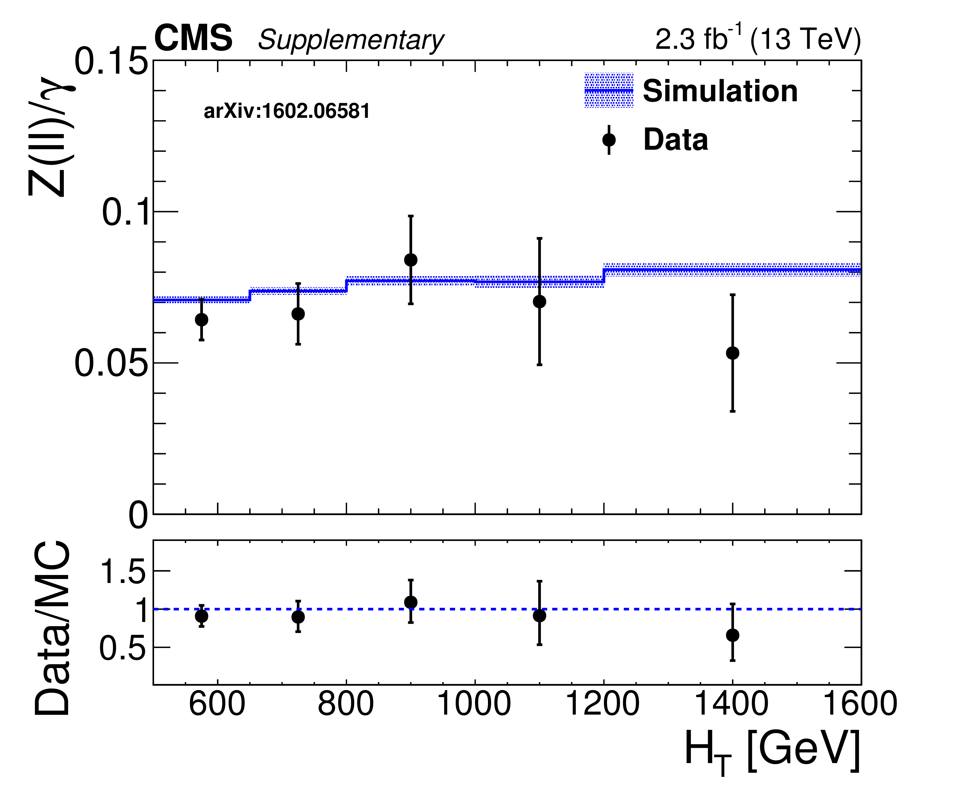
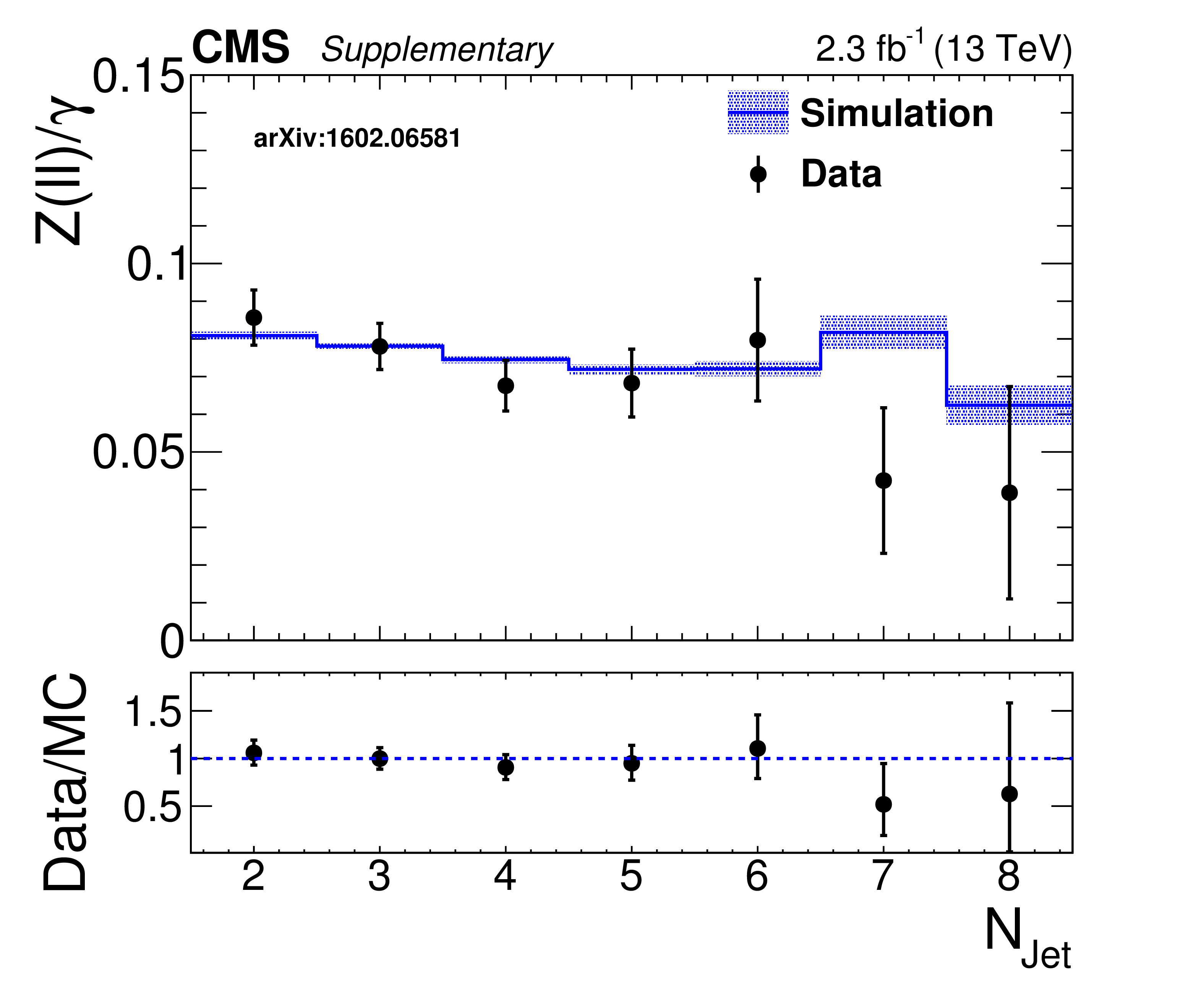
Additional Figure 13-a:
The $\mathrm{Z}\rightarrow \ell ^+\ell ^-/\gamma $ ratio as a function of $H_{\mathrm T}^{\mathrm miss}$, $H_{\mathrm T}$, and the number of jets after baseline selection. The $\mathrm{Z}\rightarrow \nu \bar{\nu}/\gamma $ transfer factor is computed using simulated events and we check in one dimensional projections that data agree with simulation. |
png pdf |
Additional Figure 13-b:
The $\mathrm{Z}\rightarrow \ell ^+\ell ^-/\gamma $ ratio as a function of $H_{\mathrm T}^{\mathrm miss}$, $H_{\mathrm T}$, and the number of jets after baseline selection. The $\mathrm{Z}\rightarrow \nu \bar{\nu}/\gamma $ transfer factor is computed using simulated events and we check in one dimensional projections that data agree with simulation. |
png pdf |
Additional Figure 13-c:
The $\mathrm{Z}\rightarrow \ell ^+\ell ^-/\gamma $ ratio as a function of $H_{\mathrm T}^{\mathrm miss}$, $H_{\mathrm T}$, and the number of jets after baseline selection. The $\mathrm{Z}\rightarrow \nu \bar{\nu}/\gamma $ transfer factor is computed using simulated events and we check in one dimensional projections that data agree with simulation. |
png pdf |
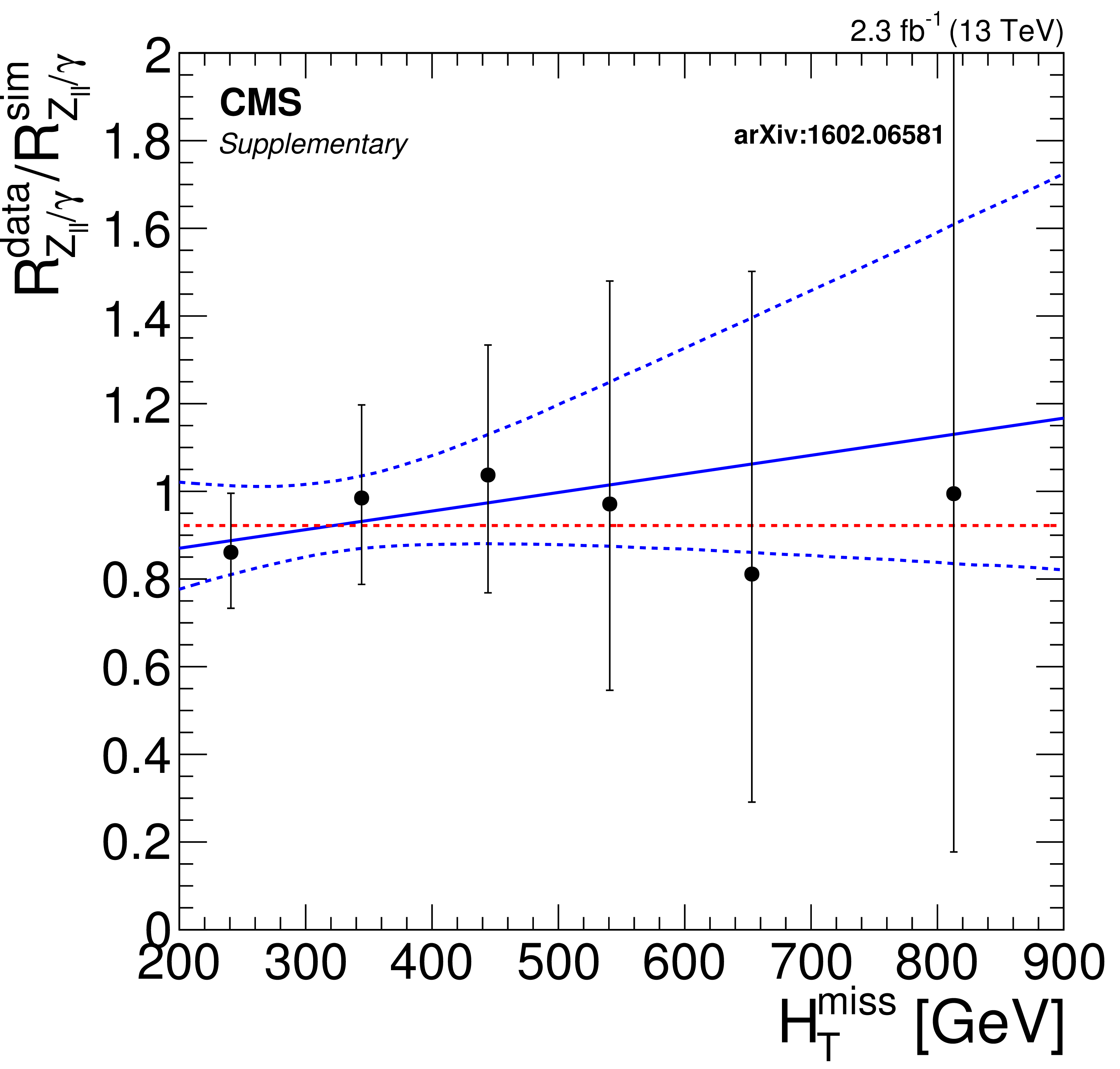
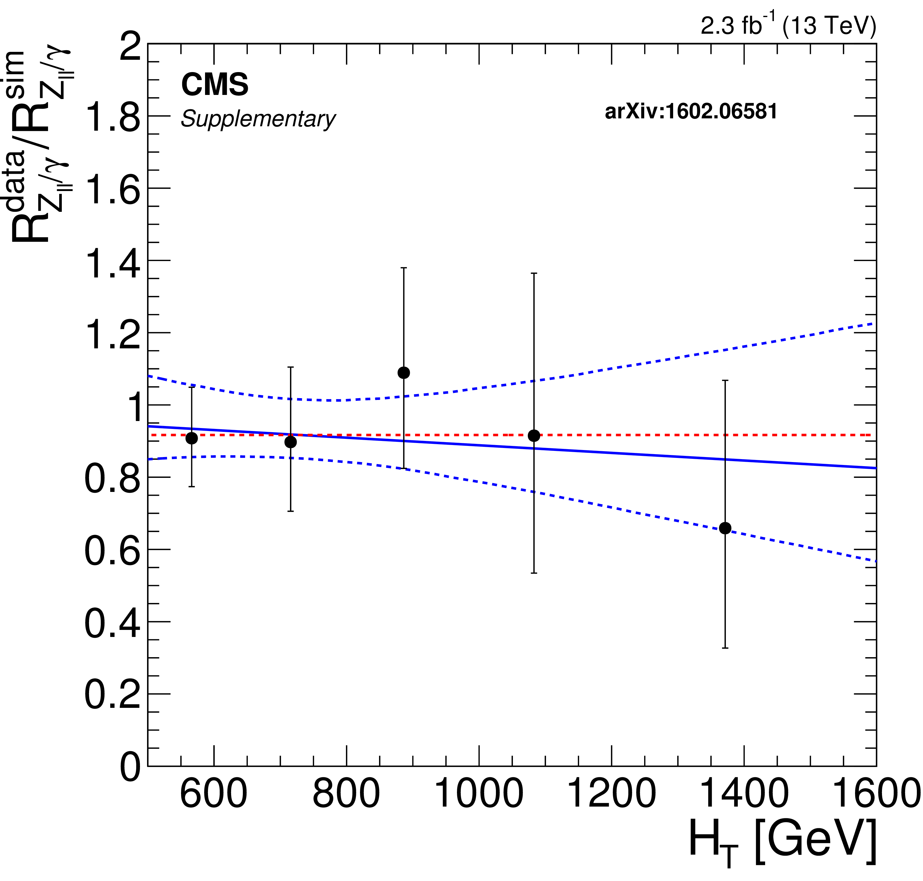
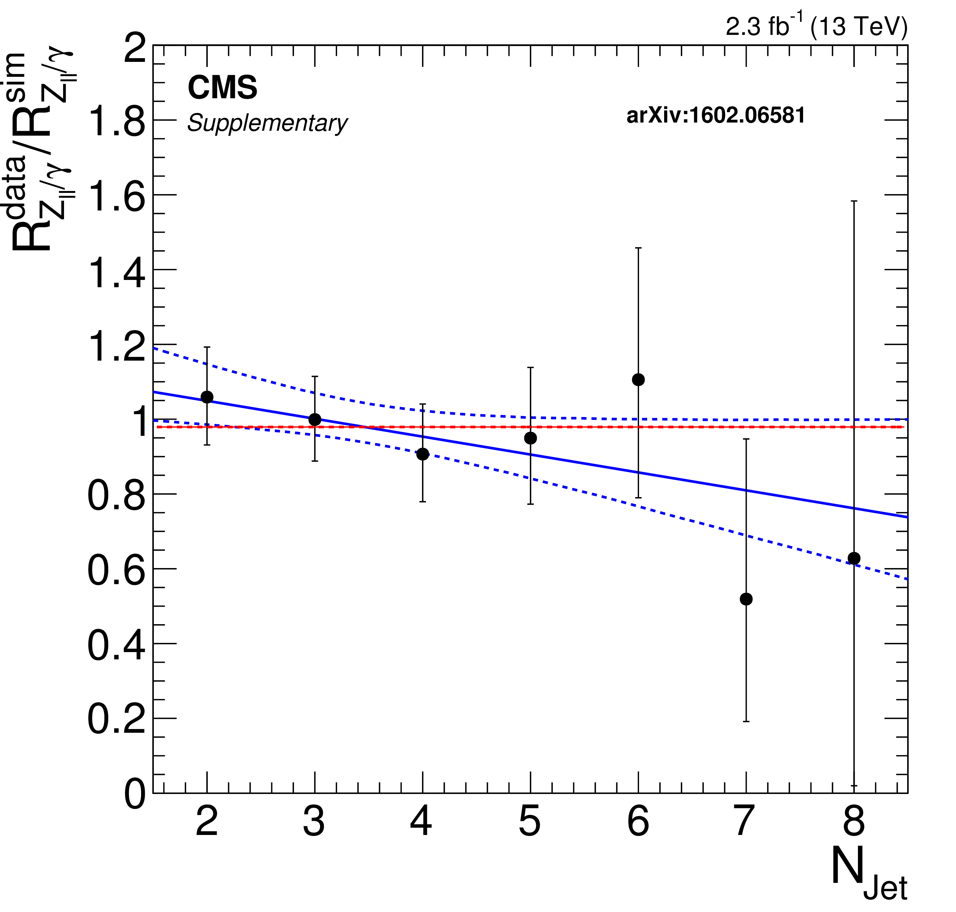
Additional Figure 14-a:
The $\mathrm{Z}\rightarrow \ell ^+\ell ^-/\gamma $ Double Ratio and linear fit as a function of $H_{\mathrm T}^{\mathrm miss}$, $H_{\mathrm T}$, and the number of jets after baseline selection. The average value of 0.924 is drawn as a red dashed line. |
png pdf |
Additional Figure 14-b:
The $\mathrm{Z}\rightarrow \ell ^+\ell ^-/\gamma $ Double Ratio and linear fit as a function of $H_{\mathrm T}^{\mathrm miss}$, $H_{\mathrm T}$, and the number of jets after baseline selection. The average value of 0.924 is drawn as a red dashed line. |
png pdf |
Additional Figure 14-c:
The $\mathrm{Z}\rightarrow \ell ^+\ell ^-/\gamma $ Double Ratio and linear fit as a function of $H_{\mathrm T}^{\mathrm miss}$, $H_{\mathrm T}$, and the number of jets after baseline selection. The average value of 0.924 is drawn as a red dashed line. |
png pdf |
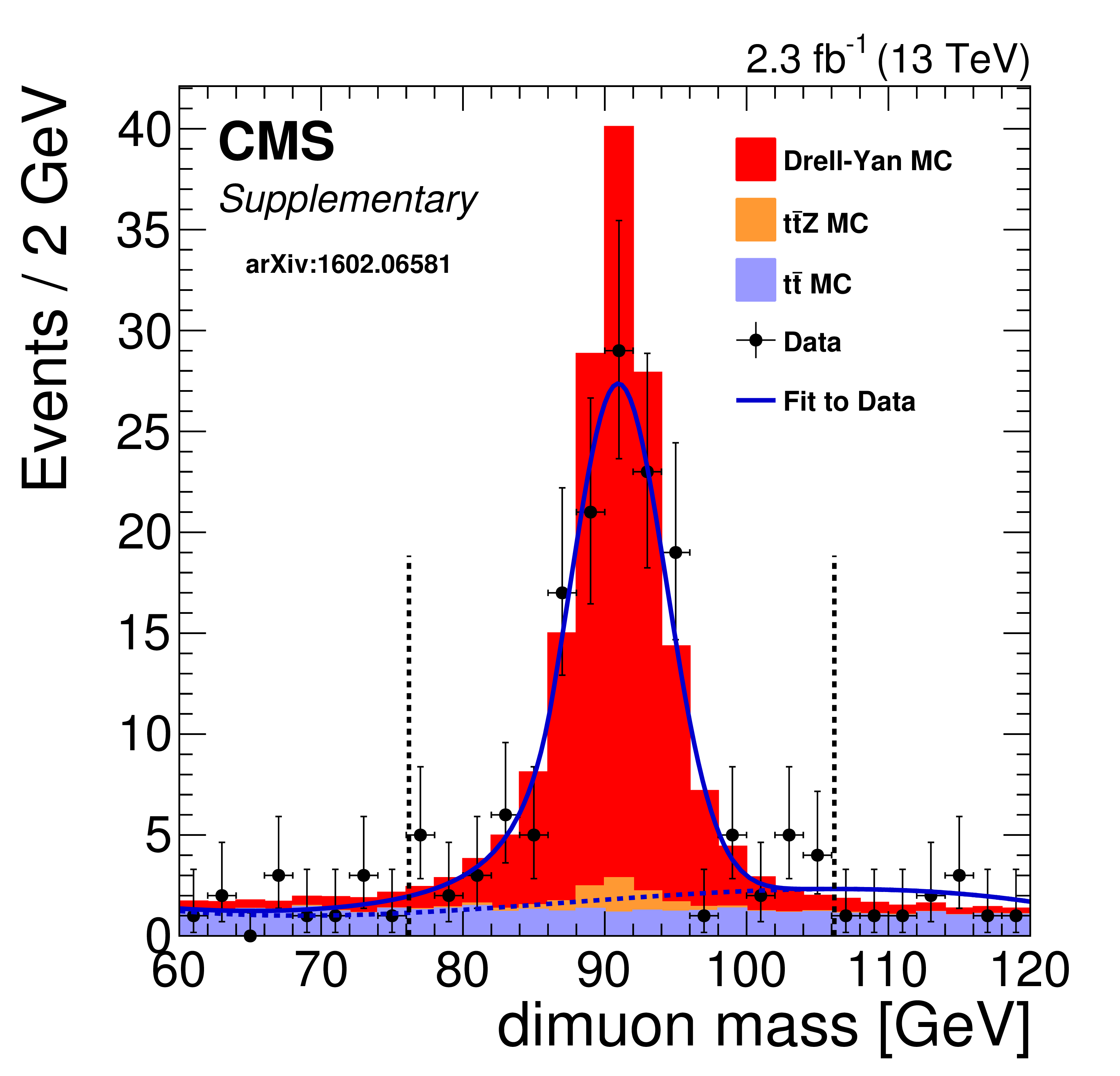
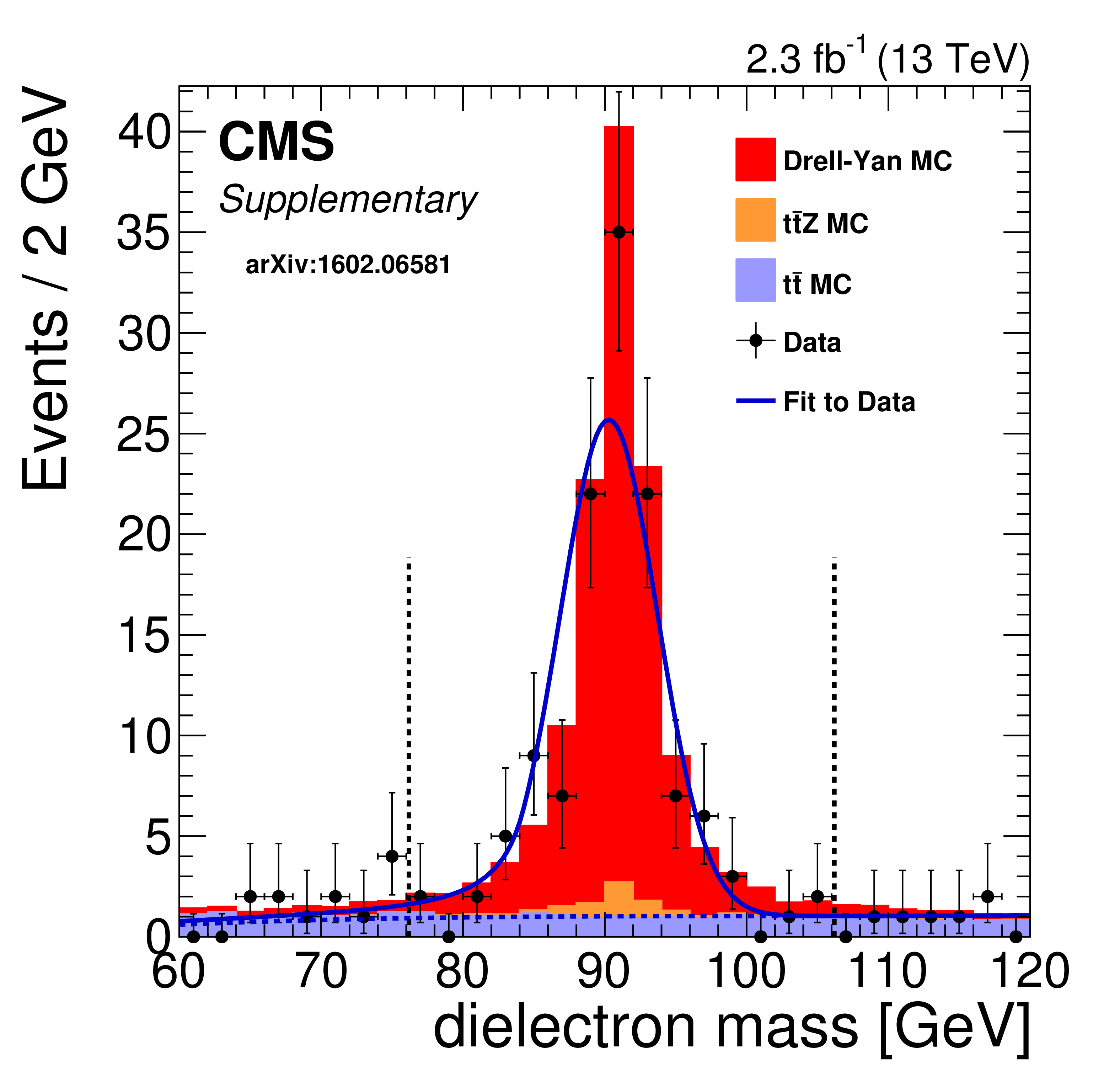
Additional Figure 15-a:
The dimuon and dielectron invariant mass distributions of the $\mathrm{Z}\rightarrow \ell ^+\ell ^-$ control regions. Fit shapes are obtained from a data sample with baseline selection, except for a loosening of the selection on the number of jets to 2. These shapes are then fixed and fit to the baseline selection as shown. |
png pdf |
Additional Figure 15-b:
The dimuon and dielectron invariant mass distributions of the $\mathrm{Z}\rightarrow \ell ^+\ell ^-$ control regions. Fit shapes are obtained from a data sample with baseline selection, except for a loosening of the selection on the number of jets to 2. These shapes are then fixed and fit to the baseline selection as shown. |
png pdf |
Additional Figure 16:
Predicted $(\mathrm{Z}\rightarrow \nu \bar{\nu})+\mathrm {jets}$ yields in the full 72-bin search space, from $\gamma +\mathrm {jets}$ data (for 0 b-tagged jets) combined with the extrapolation factors from $(\mathrm{Z}\rightarrow \ell ^+\ell ^-)+\mathrm {jets}$ (for at least 1 b-tagged jet). Statistical (blue error bars) and systematic (pink shaded) uncertainties are plotted separately, and for comparison the expectation from simulation is overlaid as the black points with (statistical) error bars. |

png pdf |
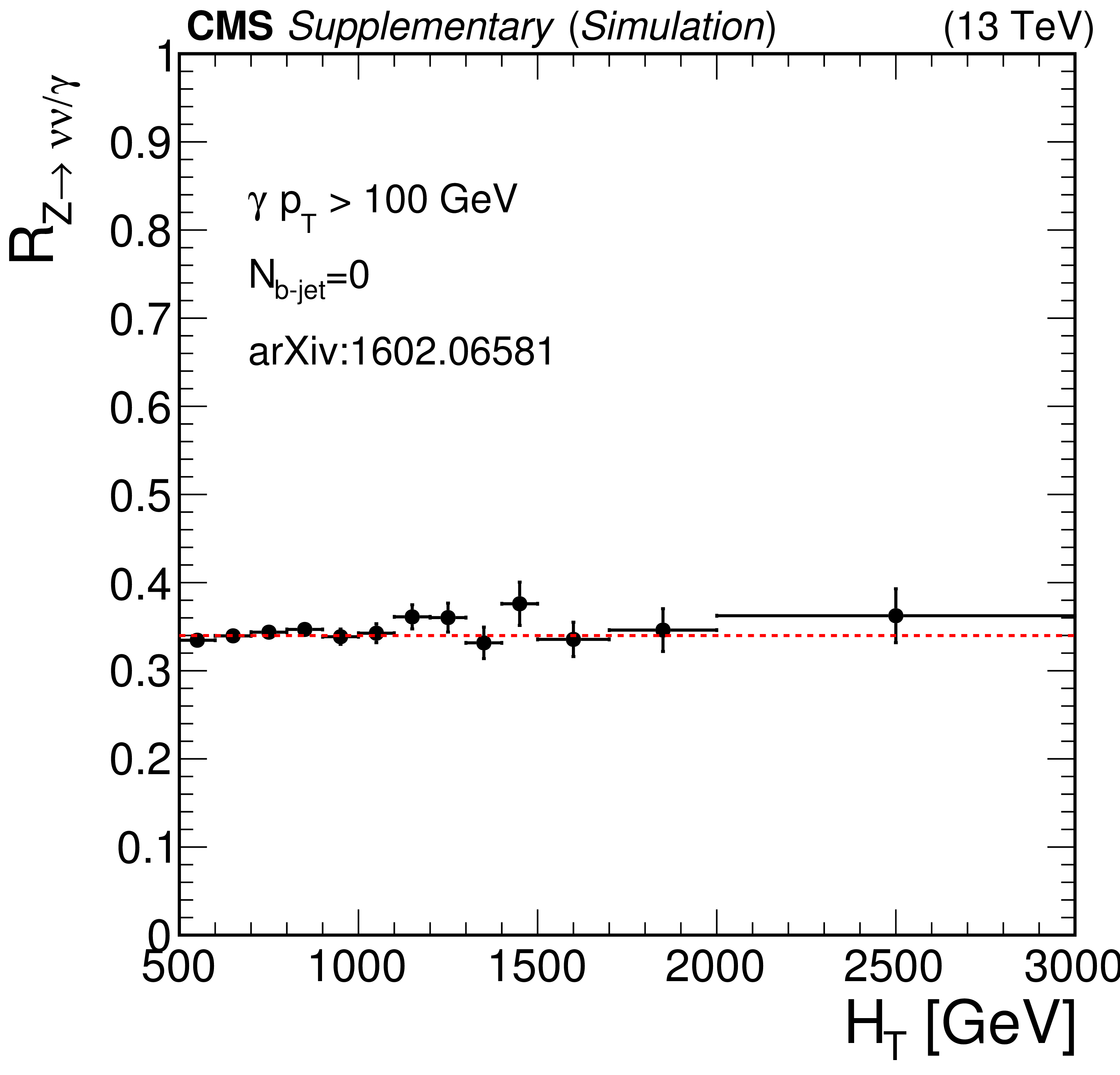
Additional Figure 17:
The $\mathrm {Z}(\nu \nu )/\gamma $ ratio calculated using leading order Monte Carlo simulation in the search bins with $N_{\mathrm {b-jet}}= $ 0 . The average value of 0.339 is drawn as a red dashed line. |
png pdf |
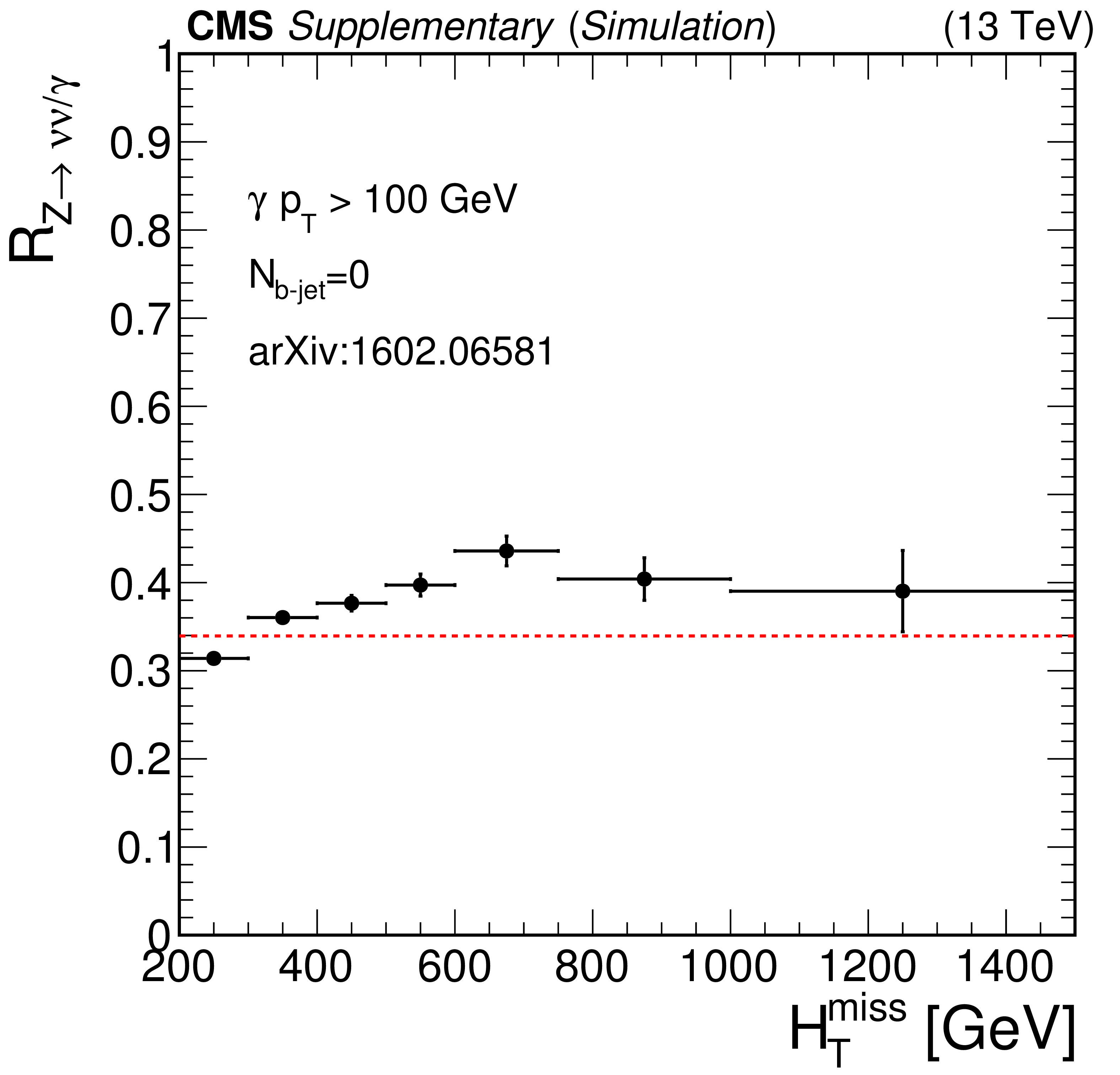
Additional Figure 18-a:
The $\mathrm {Z}(\nu \nu )/\gamma $ ratio vs. $H_{\mathrm {T}}$, $H_{\mathrm {T}}^{\mathrm {miss}}$, and $N_{\mathrm {jet}}$, calculated using leading order Monte Carlo simulation. The average value of 0.339 is drawn as a red dashed line. |
png pdf |
Additional Figure 18-b:
The $\mathrm {Z}(\nu \nu )/\gamma $ ratio vs. $H_{\mathrm {T}}$, $H_{\mathrm {T}}^{\mathrm {miss}}$, and $N_{\mathrm {jet}}$, calculated using leading order Monte Carlo simulation. The average value of 0.339 is drawn as a red dashed line. |

png pdf |
Additional Figure 18-c:
The $\mathrm {Z}(\nu \nu )/\gamma $ ratio vs. $H_{\mathrm {T}}$, $H_{\mathrm {T}}^{\mathrm {miss}}$, and $N_{\mathrm {jet}}$, calculated using leading order Monte Carlo simulation. The average value of 0.339 is drawn as a red dashed line. |

png |
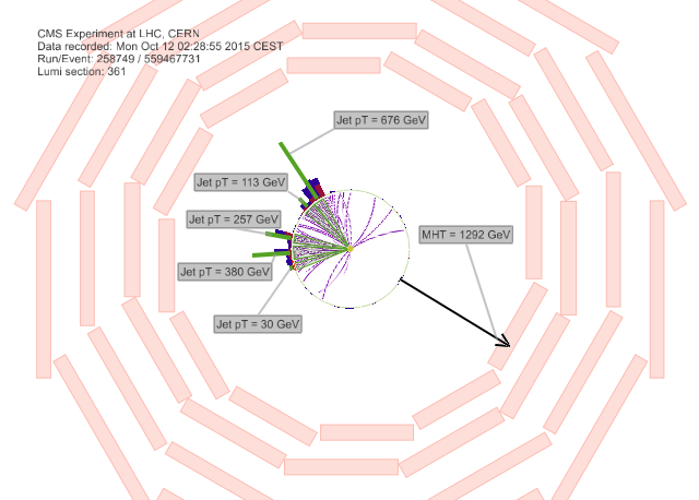
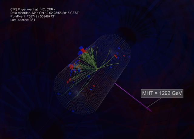
Additional Figure 19:
Event display showing the $r-\phi $ plane for event 258749:361:559467731, which has the highest observed $H_{\mathrm T}^{\mathrm miss}$ of all events in the search region. Only tracks with $p_\mathrm {T}> $ 1.5 GeV are shown. |
png |
Additional Figure 20:
Event display showing the $r-\phi $ plane for event 258749:361:559467731, with a white background. |
png |
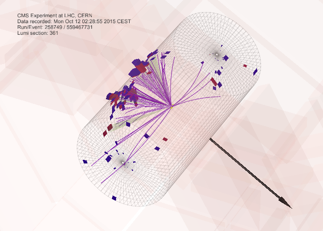
Additional Figure 21:
Event display showing event 258749:361:559467731 in 3D Tower view mode.. |
png |
Additional Figure 22:
Event display showing event 258749:361:559467731 in 3D Tower view mode with a white background. |
png pdf |
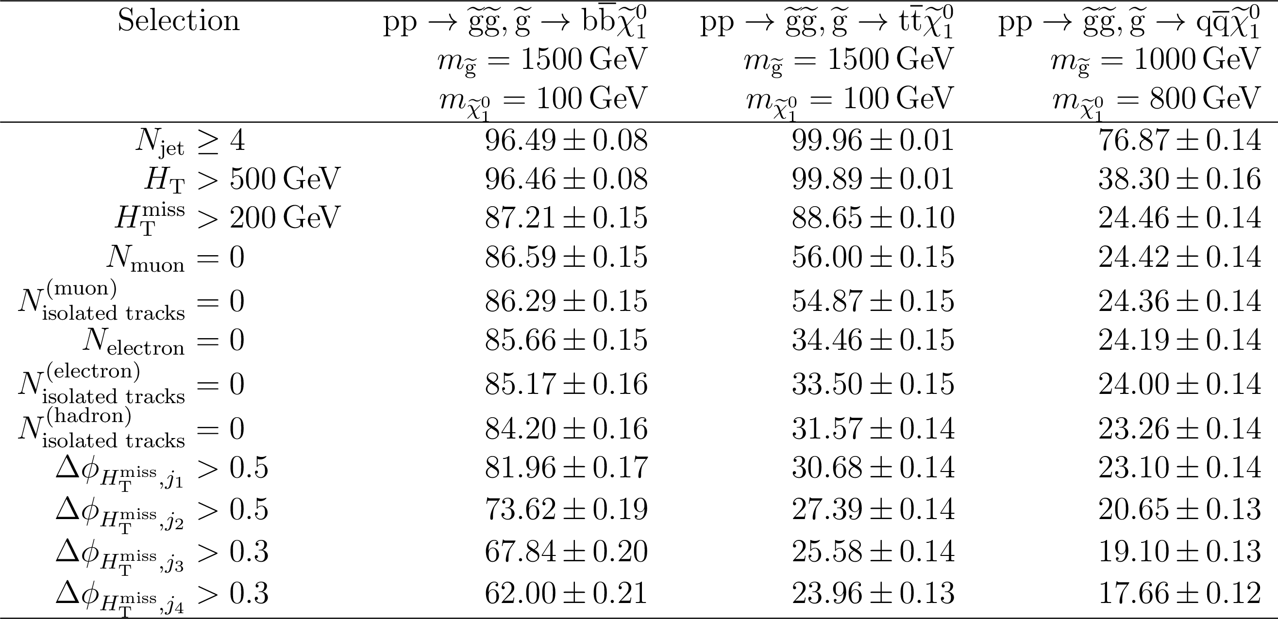
Additional Figure 23:
An expanded and reorganized version of the table of absolute cumulative efficiencies in % for each step of the event selection process, listed for three representative signal models and choices for the gluino and LSP masses. The lepton and isolated track vetoes are grouped by lepton flavor (muon or electron) and each $\Delta \phi $ cut is shown separately. Only statistical uncertainties are shown. |
png pdf root |
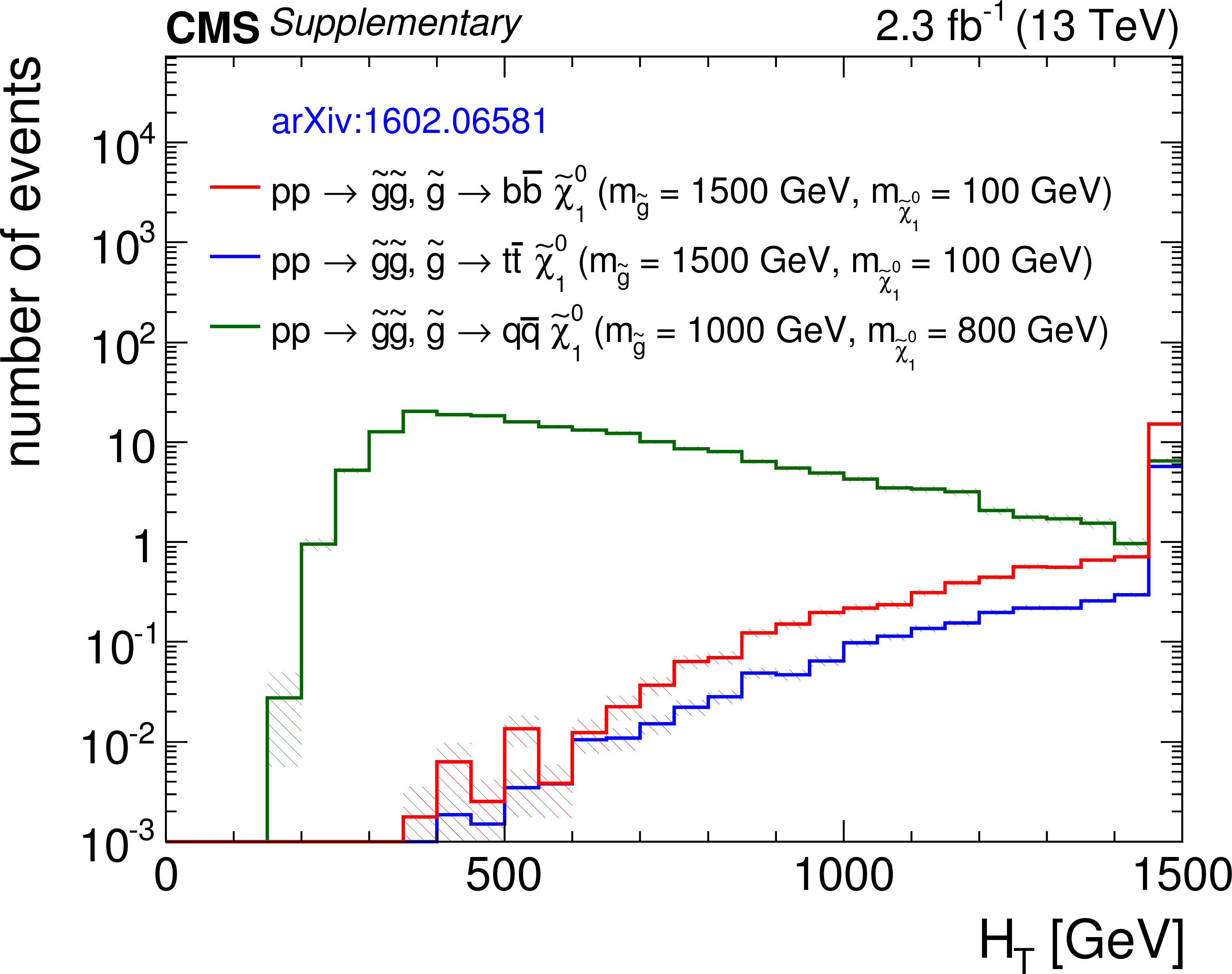
Additional Figure 24-a:
Distributions of (a) $H_{\mathrm T}$, (b) $H_{\mathrm T}^{\mathrm miss}$, (c) the number of b-tagged jets, and (d) the number of jets from three representative signal models after the baseline selection. Electronic versions of the histograms in each plot are provided as root files ('root' links). Each plot ignores the baseline requirement (if any) for its respective variable. The last bin in each plot contains the overflow events. Only statistical uncertainties are shown. |

png pdf root |
Additional Figure 24-b:
Distributions of (a) $H_{\mathrm T}$, (b) $H_{\mathrm T}^{\mathrm miss}$, (c) the number of b-tagged jets, and (d) the number of jets from three representative signal models after the baseline selection. Electronic versions of the histograms in each plot are provided as root files ('root' links). Each plot ignores the baseline requirement (if any) for its respective variable. The last bin in each plot contains the overflow events. Only statistical uncertainties are shown. |
png pdf root |
Additional Figure 24-c:
Distributions of (a) $H_{\mathrm T}$, (b) $H_{\mathrm T}^{\mathrm miss}$, (c) the number of b-tagged jets, and (d) the number of jets from three representative signal models after the baseline selection. Electronic versions of the histograms in each plot are provided as root files ('root' links). Each plot ignores the baseline requirement (if any) for its respective variable. The last bin in each plot contains the overflow events. Only statistical uncertainties are shown. |
png pdf root |
Additional Figure 24-d:
Distributions of (a) $H_{\mathrm T}$, (b) $H_{\mathrm T}^{\mathrm miss}$, (c) the number of b-tagged jets, and (d) the number of jets from three representative signal models after the baseline selection. Electronic versions of the histograms in each plot are provided as root files ('root' links). Each plot ignores the baseline requirement (if any) for its respective variable. The last bin in each plot contains the overflow events. Only statistical uncertainties are shown. |

png pdf root |
Additional Figure 25-a:
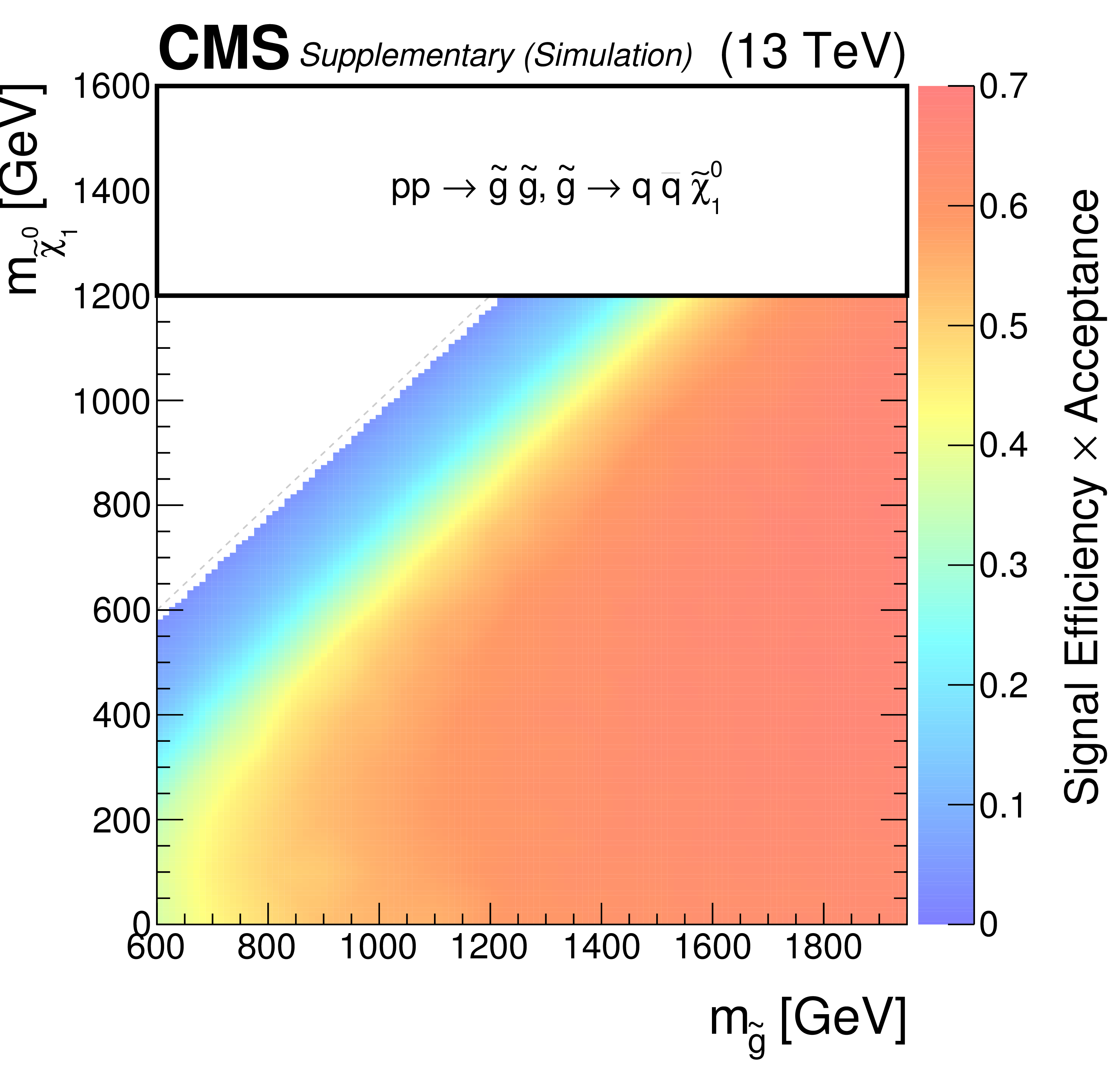
The product of signal efficiency and acceptance for the baseline selection in the $m_{\mathrm{ \tilde{g} }}-m_{\tilde{\chi}_{1}^{0}}$ mass plane for the SMS models (a) T1bbbb, (b) T1tttt, (c) T1qqqq, and (d) T5qqqqVV. Electronic versions of these figures are provided as a single root file ('root' link). |

png pdf root |
Additional Figure 25-b:
The product of signal efficiency and acceptance for the baseline selection in the $m_{\mathrm{ \tilde{g} }}-m_{\tilde{\chi}_{1}^{0}}$ mass plane for the SMS models (a) T1bbbb, (b) T1tttt, (c) T1qqqq, and (d) T5qqqqVV. Electronic versions of these figures are provided as a single root file ('root' link). |
png pdf root |
Additional Figure 25-c:
The product of signal efficiency and acceptance for the baseline selection in the $m_{\mathrm{ \tilde{g} }}-m_{\tilde{\chi}_{1}^{0}}$ mass plane for the SMS models (a) T1bbbb, (b) T1tttt, (c) T1qqqq, and (d) T5qqqqVV. Electronic versions of these figures are provided as a single root file ('root' link). |

png pdf root |
Additional Figure 25-d:
The product of signal efficiency and acceptance for the baseline selection in the $m_{\mathrm{ \tilde{g} }}-m_{\tilde{\chi}_{1}^{0}}$ mass plane for the SMS models (a) T1bbbb, (b) T1tttt, (c) T1qqqq, and (d) T5qqqqVV. Electronic versions of these figures are provided as a single root file ('root' link). |
png pdf |
Additional Figure 26:
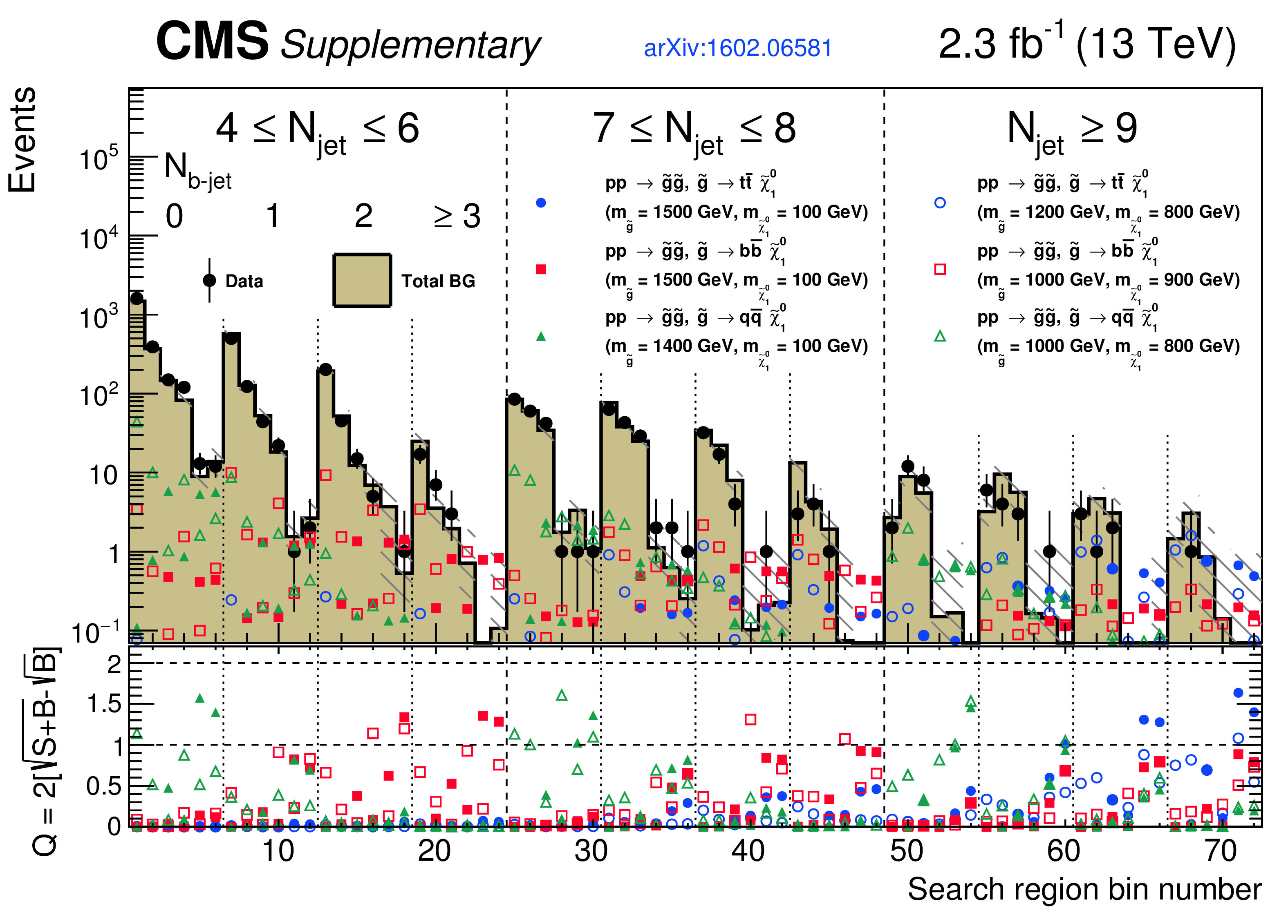
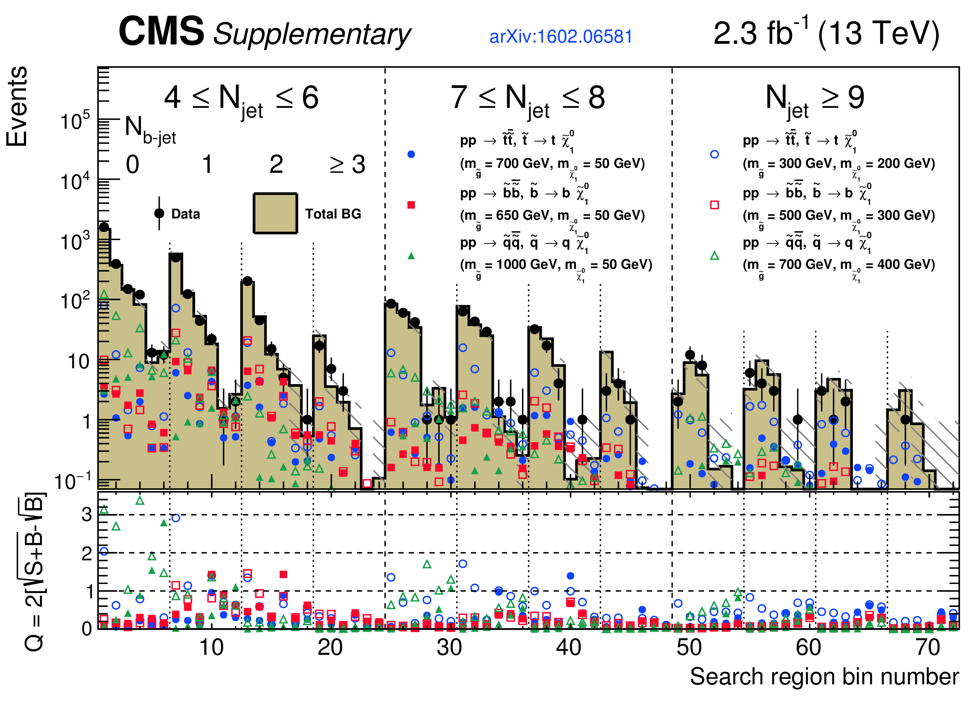
The sensitivity of the analysis to different direct gluino production signal models as a function of the analysis binning. The upper panel shows the total predicted SM backgrounds and the expected number of signal events for six representative model points per analysis bin. The bottom panel shows the expected sensitivity, expressed in terms of the figure of merit Q, per analysis bin. |
png pdf |
Additional Figure 27:
The sensitivity of the analysis to different direct squark production signal models as a function of the analysis binning. The upper panel shows the total predicted SM backgrounds and the expected number of signal events for six representative model points per analysis bin. The bottom panel shows the expected sensitivity, expressed in terms of the figure of merit Q, per analysis bin. |
png pdf |
Additional Figure 28:
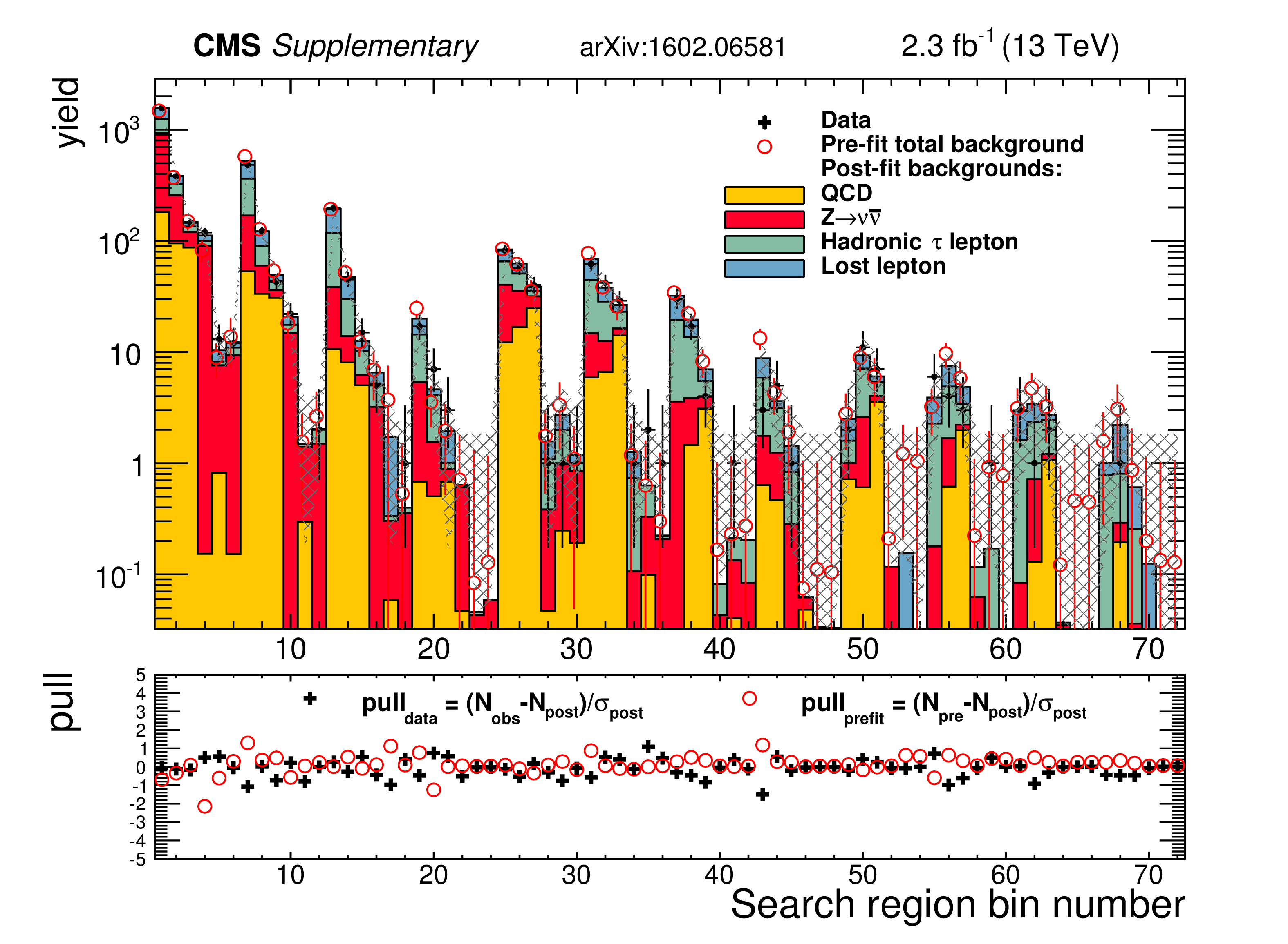
Observed numbers of events and corresponding SM background predictions in the 72 search regions of the analysis after the final fit performed with the assumption of only standard model contributions. Background predictions before the final fit are also shown for comparison. The lower panel shows the pull distributions for the data and the pre-fit background estimates with respect to the post-fit background estimates. |
png pdf |
Additional Figure 29-a:
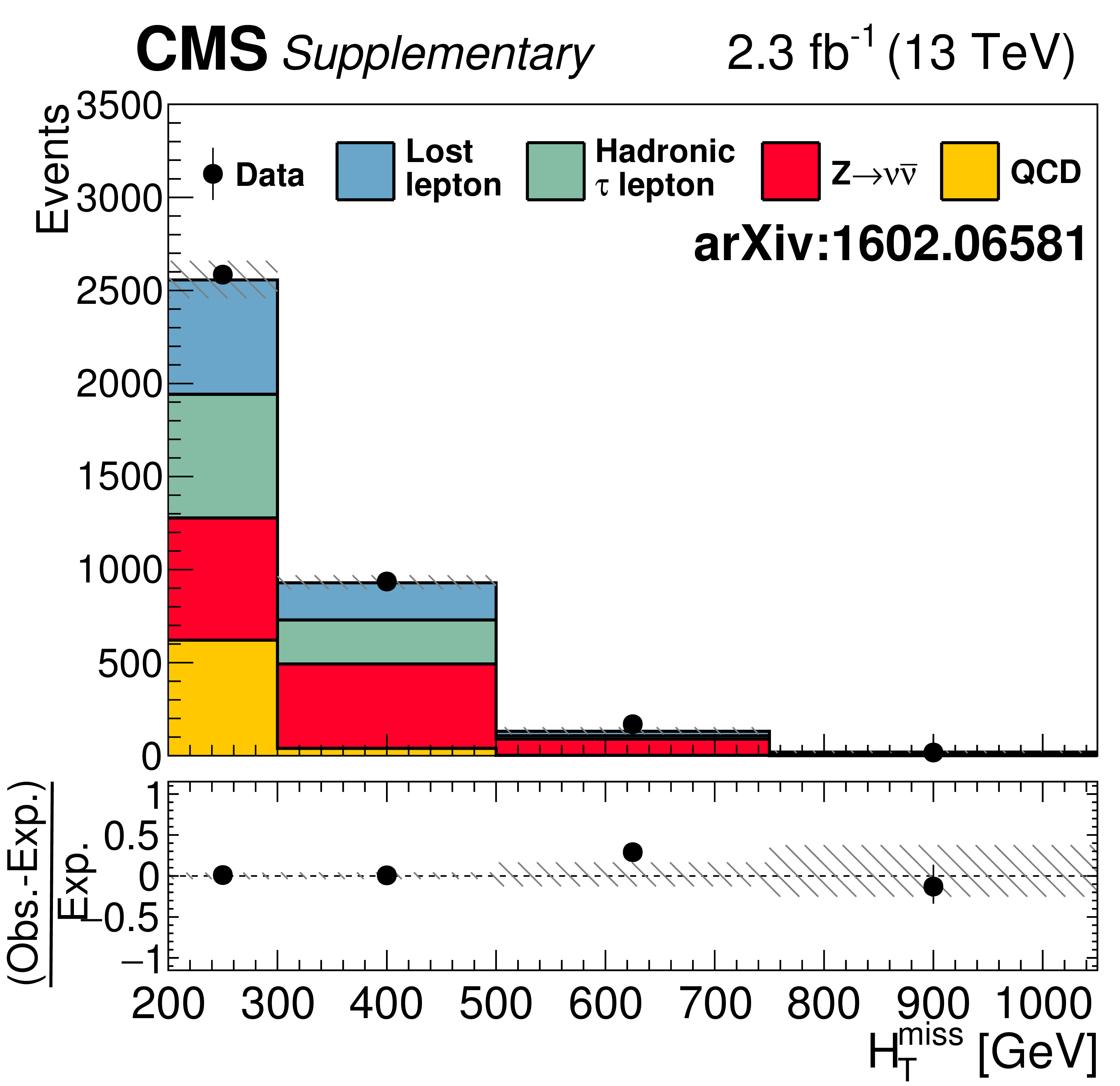
The distributions of observed number of events and predicted background as a function of $H_{\mathrm T}^{\mathrm miss}$, plotted on linear and log scales. Distributions are integrated over other binned observables in the analysis, number of b-tagged jets, number of jets, and $H_{\mathrm T}$. |

png pdf |
Additional Figure 29-b:
The distributions of observed number of events and predicted background as a function of $H_{\mathrm T}^{\mathrm miss}$, plotted on linear and log scales. Distributions are integrated over other binned observables in the analysis, number of b-tagged jets, number of jets, and $H_{\mathrm T}$. |

png pdf |
Additional Figure 30-a:
The distributions of observed number of events and predicted background as a function of $H_{\mathrm T}$, plotted on linear and log scales. Distributions are integrated over other binned observables in the analysis, number of b-tagged jets, number of jets, and $H_{\mathrm T}^{\mathrm miss}$. |

png pdf |
Additional Figure 30-b:
The distributions of observed number of events and predicted background as a function of $H_{\mathrm T}$, plotted on linear and log scales. Distributions are integrated over other binned observables in the analysis, number of b-tagged jets, number of jets, and $H_{\mathrm T}^{\mathrm miss}$. |
png pdf |
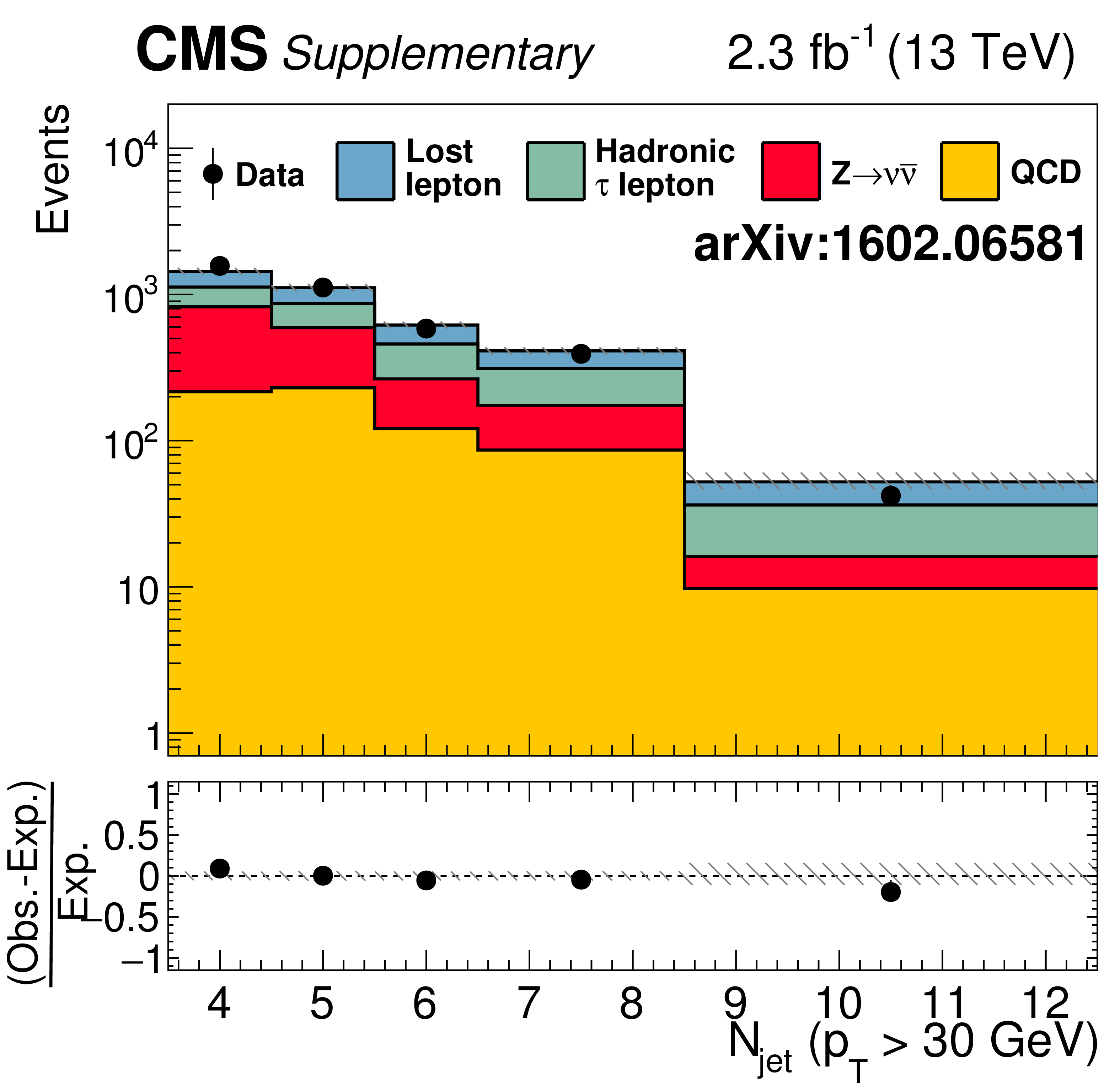
Additional Figure 31-a:
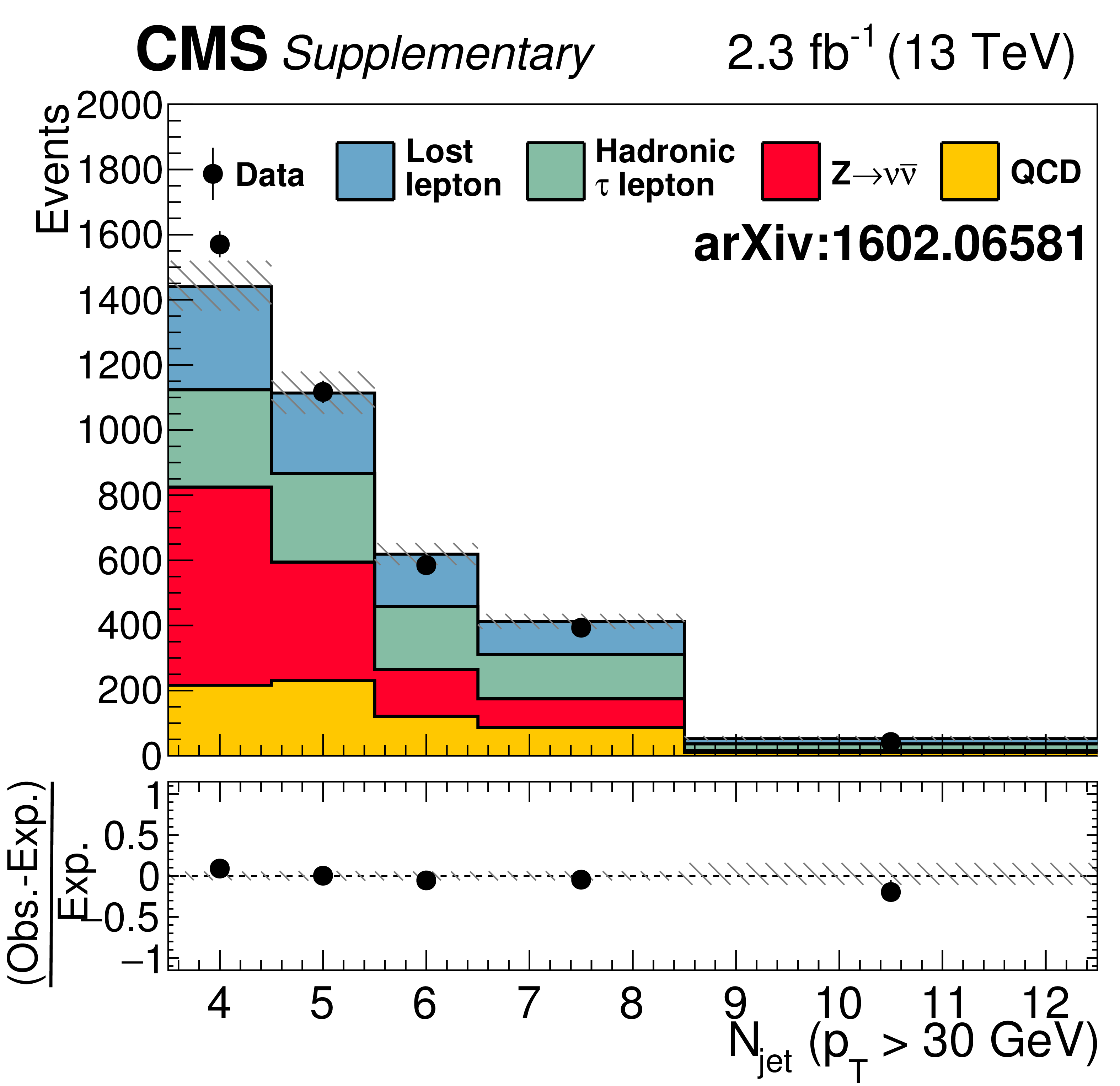
The distributions of observed number of events and predicted background as a function of the number of jets, plotted on linear and log scales. Distributions are integrated over other binned observables in the analysis, number of b-tagged jets, $H_{\mathrm T}^{\mathrm miss}$, and $H_{\mathrm T}$. |
png pdf |
Additional Figure 31-b:
The distributions of observed number of events and predicted background as a function of the number of jets, plotted on linear and log scales. Distributions are integrated over other binned observables in the analysis, number of b-tagged jets, $H_{\mathrm T}^{\mathrm miss}$, and $H_{\mathrm T}$. |

png pdf |
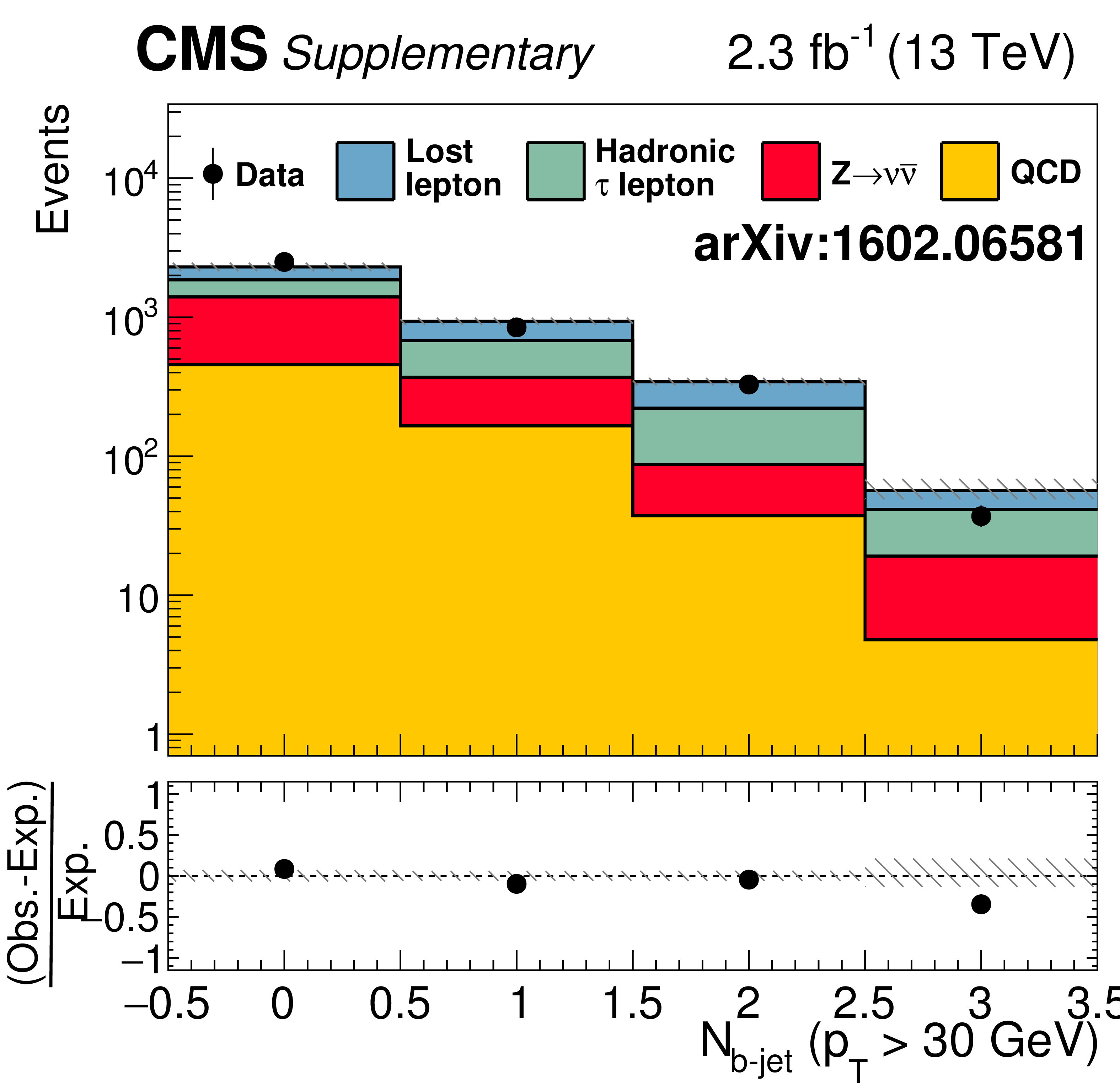
Additional Figure 32-a:
The distributions of observed number of events and predicted background as a function of the number of b-tagged jets, plotted on linear and log scales. Distributions are integrated over other binned observables in the analysis, number of jets, $H_{\mathrm T}^{\mathrm miss}$, and $H_{\mathrm T}$. |
png pdf |
Additional Figure 32-b:
The distributions of observed number of events and predicted background as a function of the number of b-tagged jets, plotted on linear and log scales. Distributions are integrated over other binned observables in the analysis, number of jets, $H_{\mathrm T}^{\mathrm miss}$, and $H_{\mathrm T}$. |
png pdf |
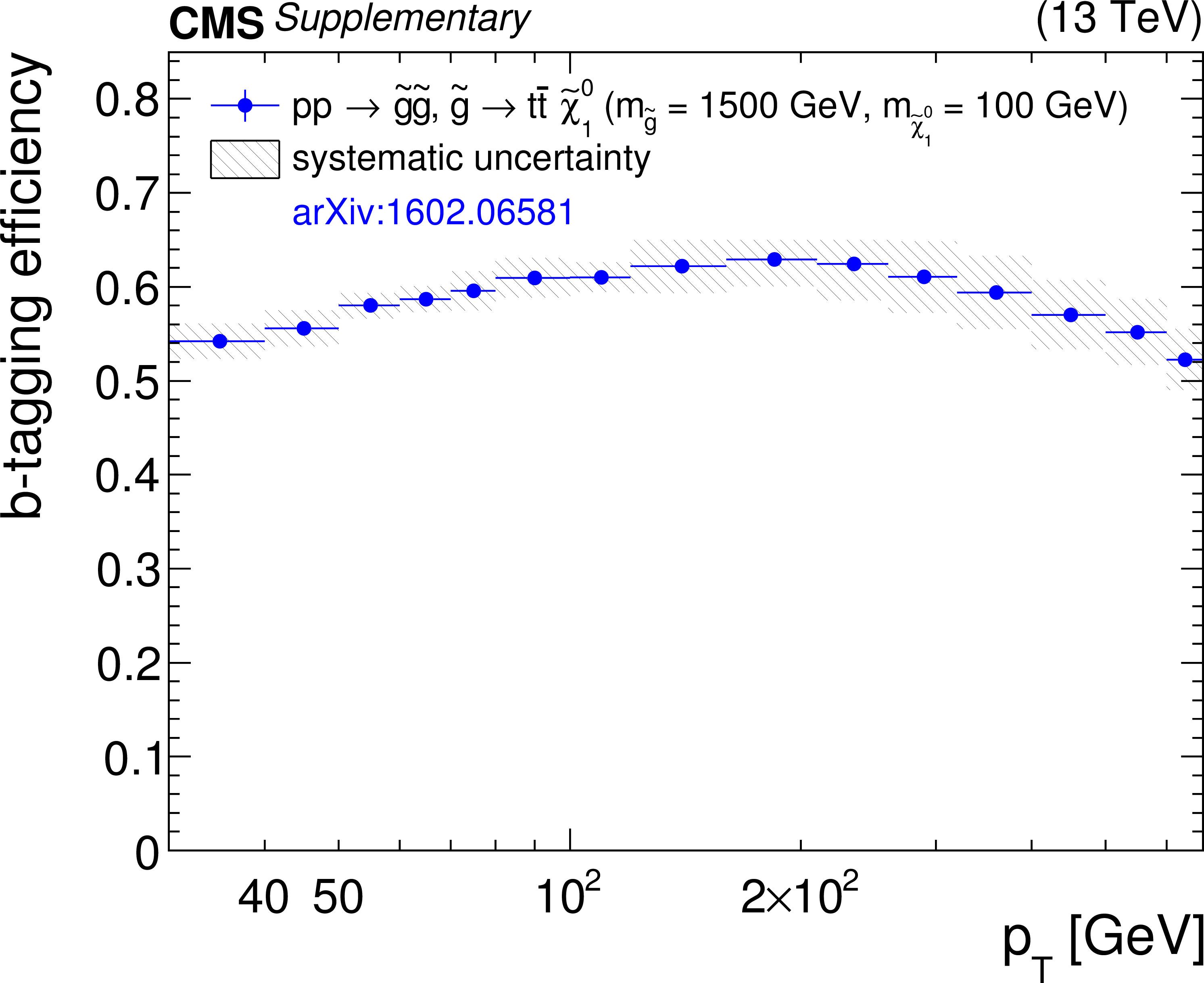
Additional Figure 33:
The b-tagging efficiency, with data/MC scale factors applied, for a representative signal model. Statistical and systematic uncertainties are shown separately. |

png pdf |
Additional Figure 34:
The b-tagging efficiency in table form, with data/MC scale factors applied, for a representative signal model. Statistical and systematic uncertainties are shown separately. |
png pdf |
Additional Figure 35-a:
Event diagrams for the T1ttbb model, with two out of its six possible topologies. |
png pdf |
Additional Figure 35-b:
Event diagrams for the T1ttbb model, with two out of its six possible topologies. |

png pdf |
Additional Figure 35-c:
Event diagrams for the T1ttbb model, with two out of its six possible topologies. |
png pdf |
Additional Figure 36:
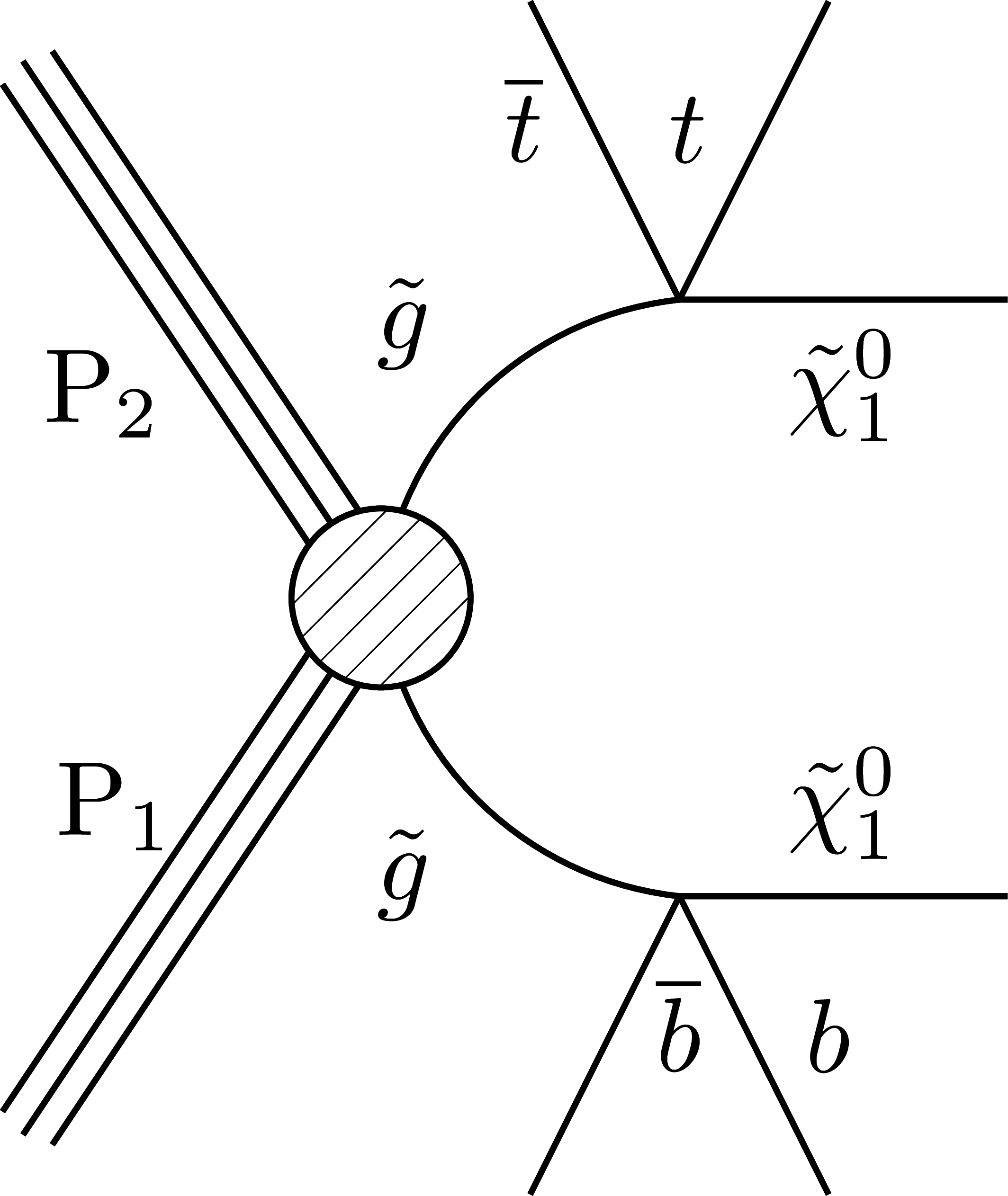
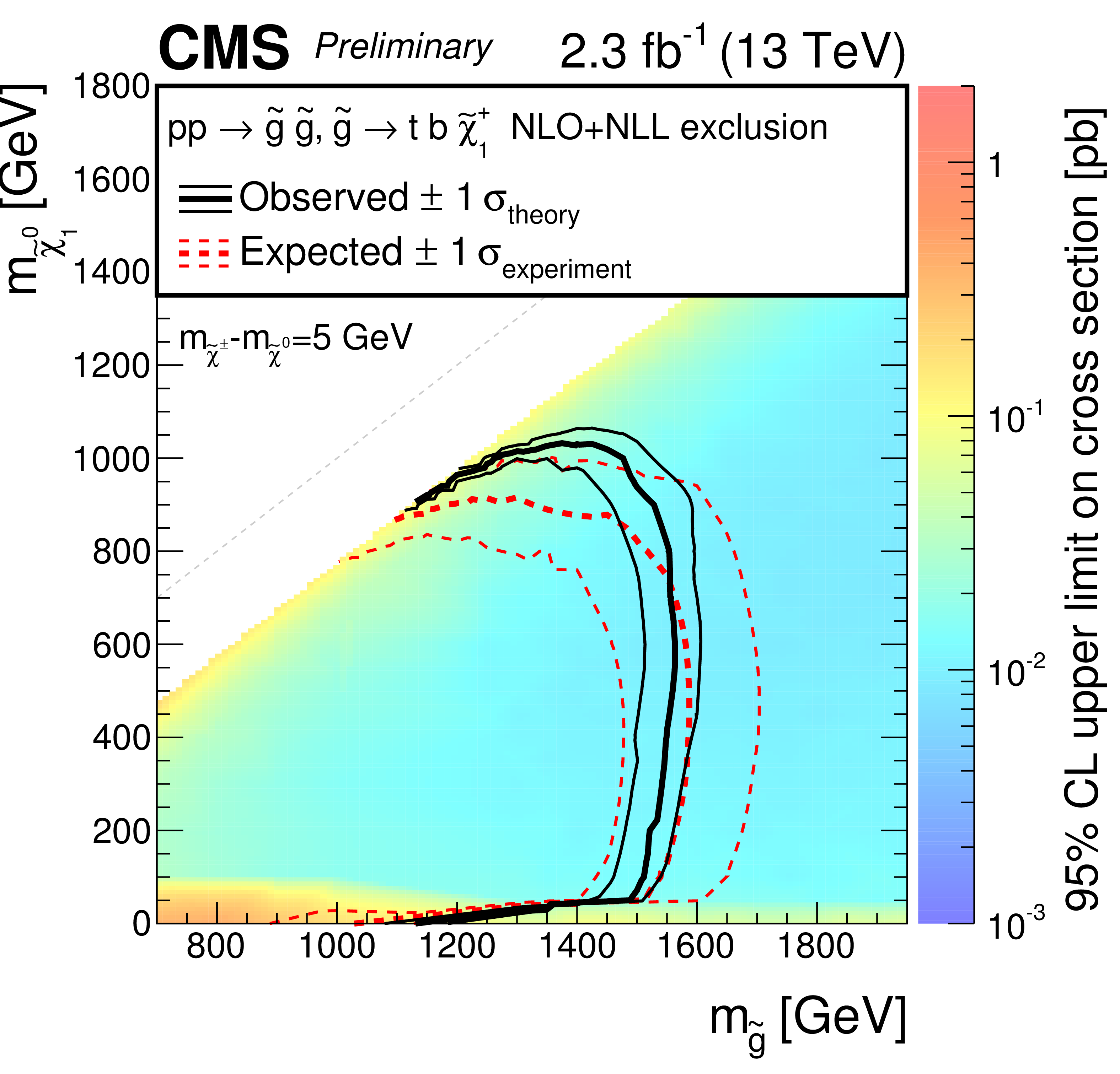
Exclusion region in the $\mathrm{ \tilde{g} } -\tilde{\chi}^0_1$ mass plane at 95% C.L., for $\mathrm{ \tilde{g} } \mathrm{ \tilde{g} }$ pair production on the T1ttbb SMS for for $\mathcal {BR}(\mathrm{ \tilde{g} } \rightarrow \mathrm{ t } \mathrm{ b } \tilde{\chi}^{pm}_1 )=100%$. |

png pdf |
Additional Figure 37:
Exclusion region in the $\mathrm{ \tilde{g} } -\tilde{\chi}^0_1$ mass plane at 95% C.L., for $ \mathrm{ \tilde{g} } \mathrm{ \tilde{g} }$ pair production on the T1ttbb SMS for different choices of the $\mathrm{ \tilde{g} } \mathrm{ \tilde{g} }$ branching ratio into top and bottom quarks. |
png pdf |
Additional Figure 38:
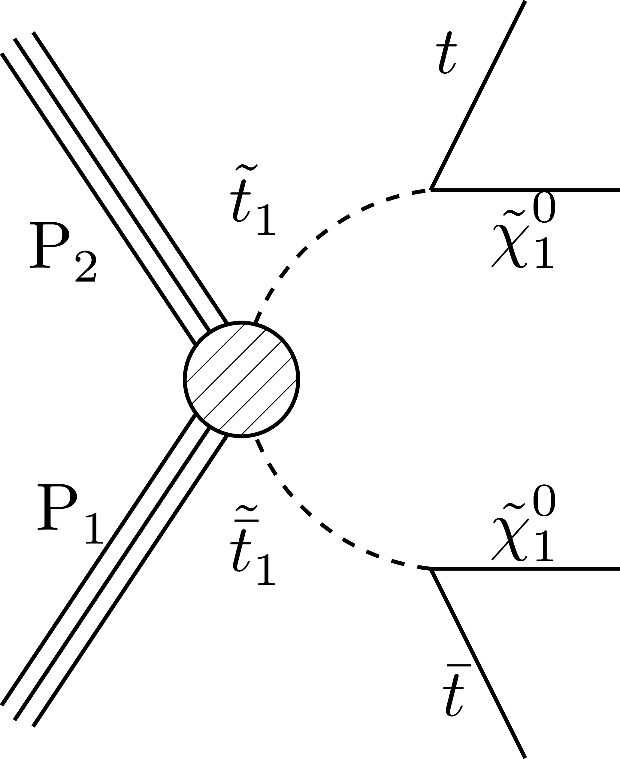
Event diagram for the direct top squark production model, T2tt. |

png pdf |
Additional Figure 39:
Upper limits and exclusion region at 95% C.L. on the $\tilde{ \mathrm{ t } } -\tilde{\chi}^0_1$ mass plane for the T2tt model. The region where $M_{\tilde{ \mathrm{ t } } } \approx M_{\mathrm{ t } }+M_{\tilde{\chi}^0_1 }$ is masked, as this region of parameter space will be targeted by a dedicated analysis. |
| Additional Tables | |

png pdf |
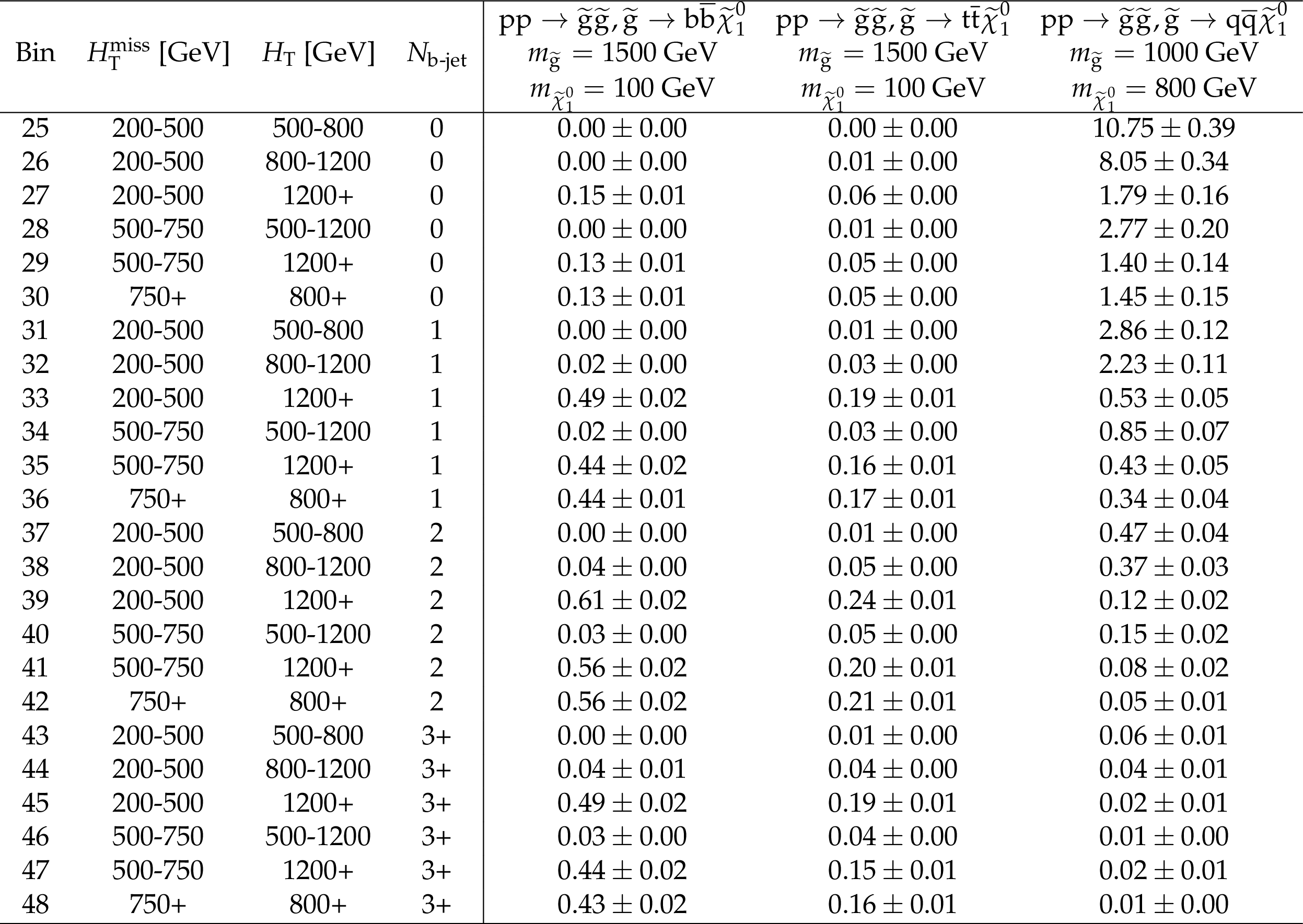
Additional Table 1:
Expected numbers of events in search bins with 4 $ \leq N_{\mathrm jet}\leq $ 6 for three representative signal models. Only statistical uncertainties are shown. |
png pdf |
Additional Table 2:
Expected numbers of events in search bins with 7 $ \leq N_{\mathrm jet}\leq $ 8 for three representative signal models. Only statistical uncertainties are shown. |

png pdf |
Additional Table 3:
Expected numbers of events in search bins with $N_{\mathrm jet}\geq $ 9 for three representative signal models. Only statistical uncertainties are shown. |
|
|
Compact Muon Solenoid LHC, CERN |
|

|

|

|

|

|