

Compact Muon Solenoid
LHC, CERN
| CMS-PAS-SUS-15-011 | ||
| Search for new physics in final states with two opposite-sign same-flavor leptons, jets and $ E_{ \mathrm{T} }^{ \text{miss} } $ in pp collisions at $ \sqrt{s} =$ 13 TeV | ||
| CMS Collaboration | ||
| December 2015 | ||
| Abstract: A search is presented for physics beyond the standard model in final states with two opposite-sign same-flavor leptons, jets, and missing transverse momentum. The data sample corresponds to an integrated luminosity of 2.2 fb$^{-1}$ of proton-proton collisions at $\sqrt{s}= $ 13 TeV collected with the CMS detector at the CERN LHC in 2015. The analysis focuses on the invariant mass distribution of the lepton pair, searching for a kinematic edge or a resonant-like excess compatible with the Z boson mass. The kinematic edge search includes phase-space regions matching the previous 8 TeV analysis where CMS reported a 2.6$\sigma$ excess. The resonant Z boson peak search includes a region where ATLAS reported a 3.0$\sigma$ excess at 8 TeV. Additional event categories are included in both searches beyond those in the 8~TeV analysis to increase sensitivity to new physics. The observations in all signal regions are consistent with the expectations from the standard model, and the results are interpreted in the context of simplified models of supersymmetry. | ||
|
Links:
CDS record (PDF) ;
CADI line (restricted) ;
These preliminary results are superseded in this paper, JHEP 12 (2016) 013. The superseded preliminary plots can be found here. |
||
| Figures | |

png ; pdf ; |
Figure 1-a:
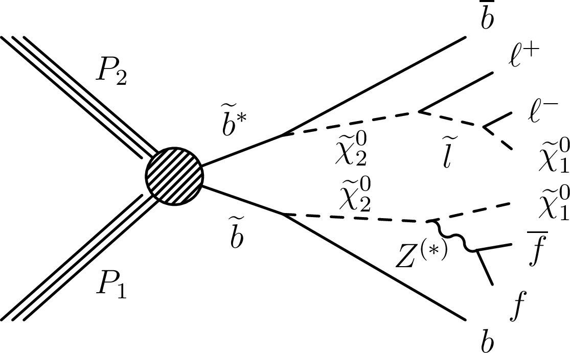
Feynman diagrams for gluino and $ \tilde{b} $ pair production and decays realized in the simplified models. The GMSB model targeted by the on-Z search is shown on (a). On (b), the slepton-edge model features characteristic edges in the $m_{\ell \ell }$ spectrum given by the mass difference of the $ \tilde{\chi }^0_2 $ and $ \tilde{\chi }^0_1 $. |
png ; pdf ; |
Figure 1-b:
Feynman diagrams for gluino and $ \tilde{b} $ pair production and decays realized in the simplified models. The GMSB model targeted by the on-Z search is shown on (a). On (b), the slepton-edge model features characteristic edges in the $m_{\ell \ell }$ spectrum given by the mass difference of the $ \tilde{\chi }^0_2 $ and $ \tilde{\chi }^0_1 $. |
png ; pdf ; |
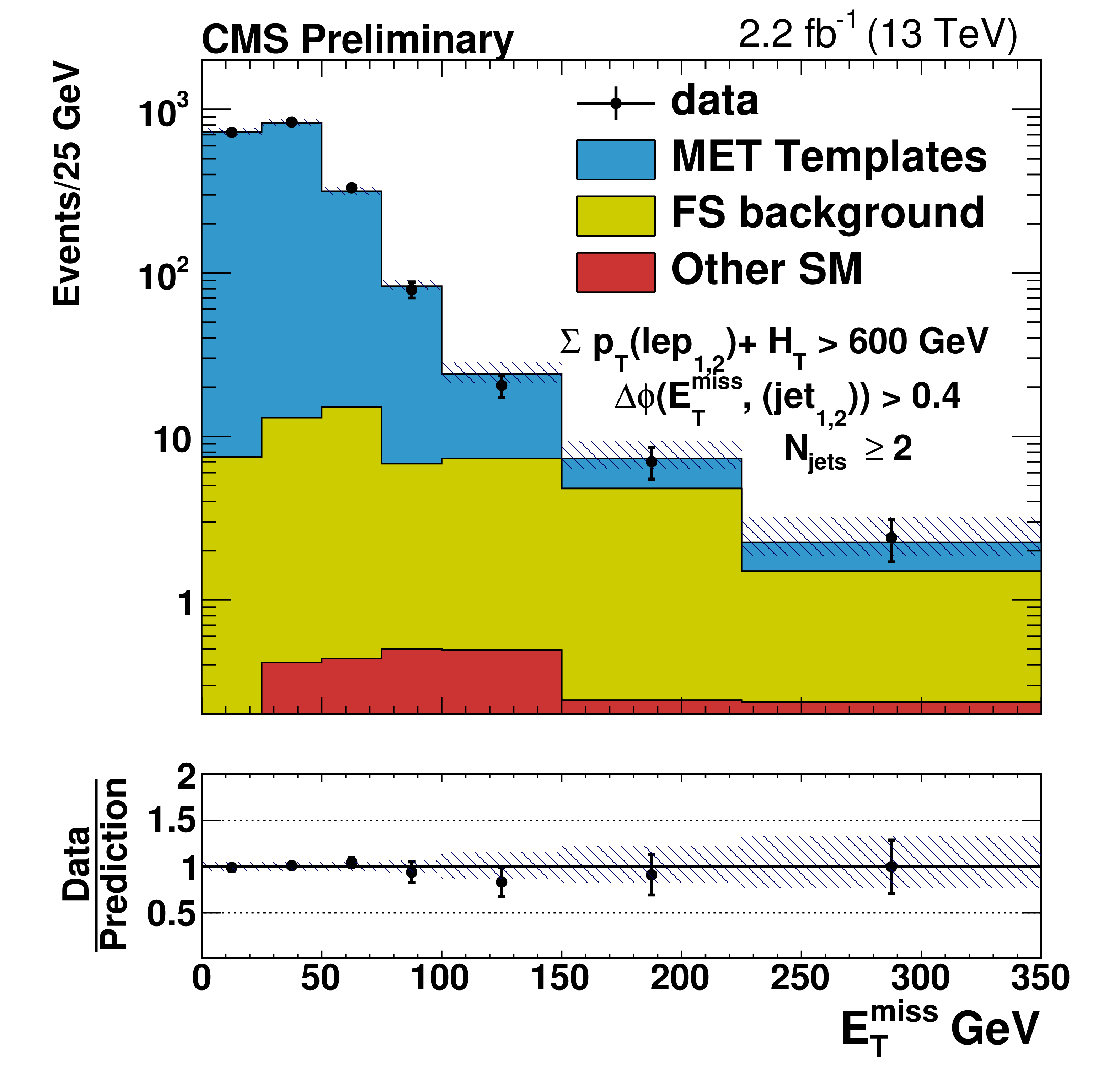
Figure 2-a:
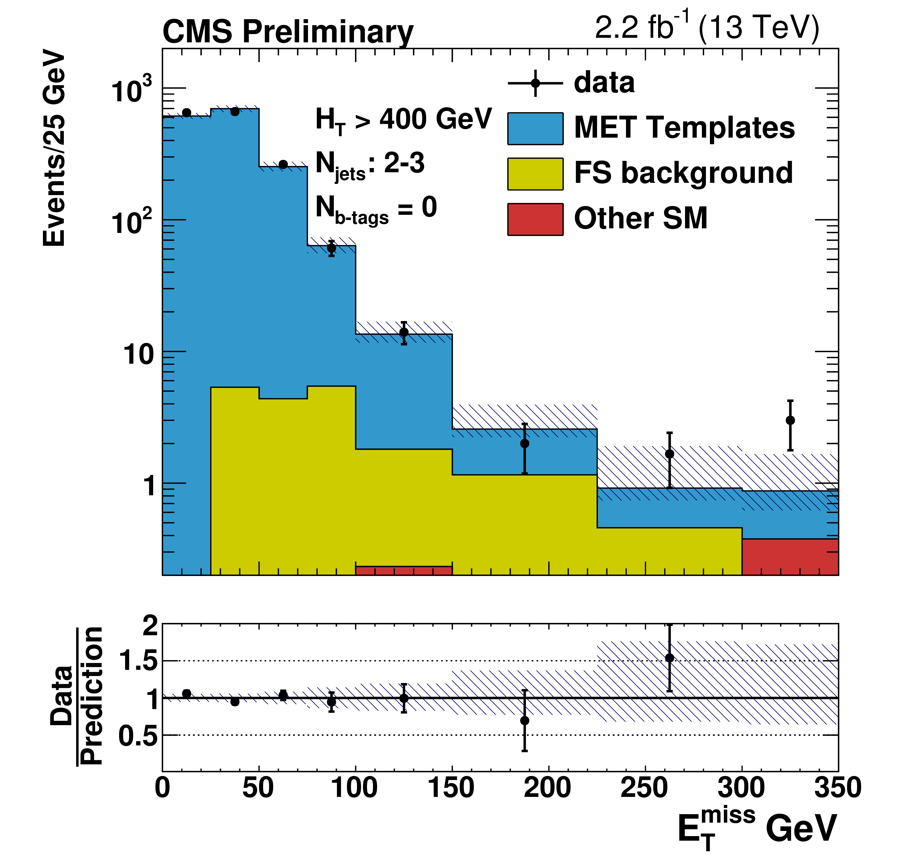
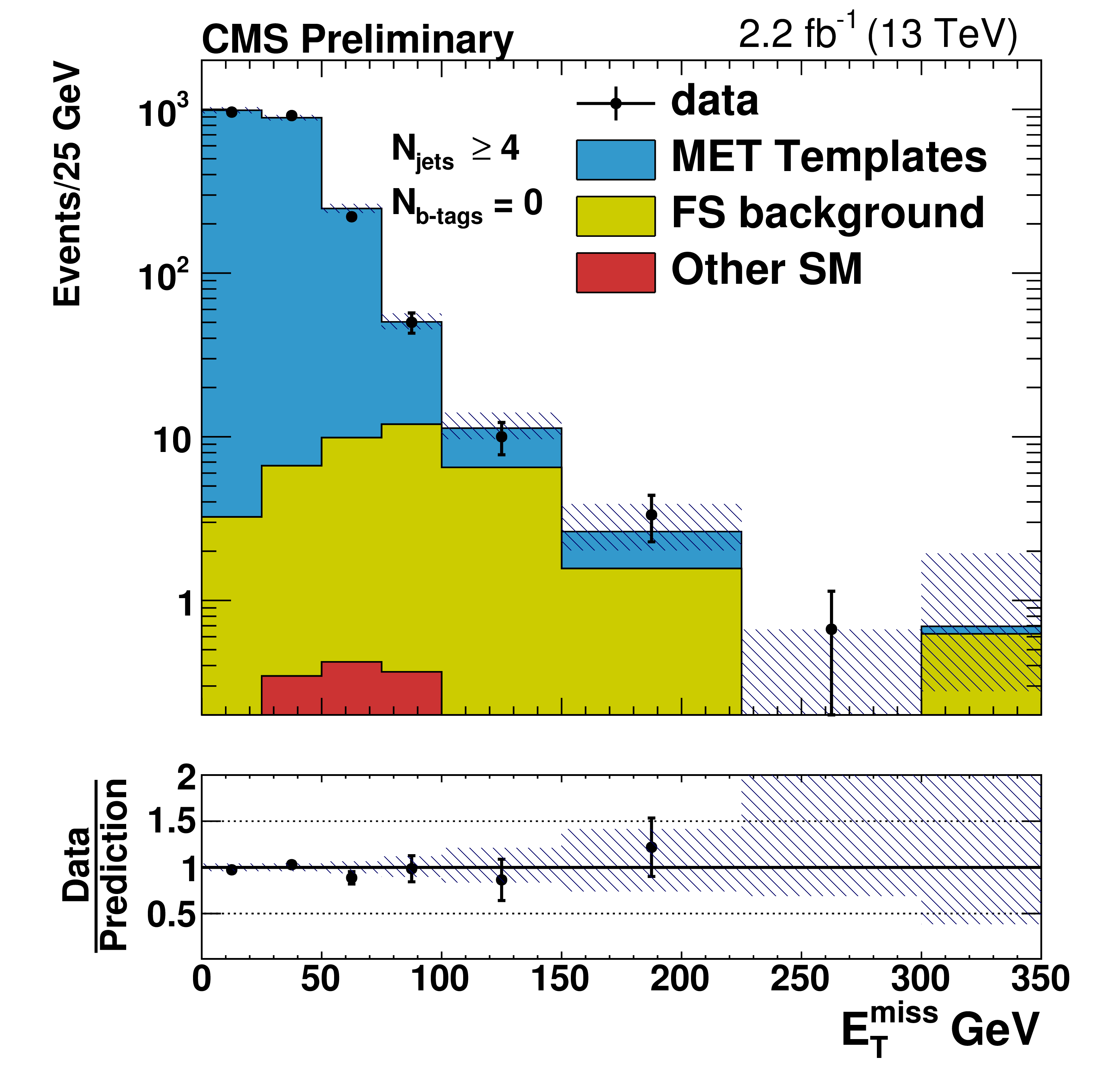
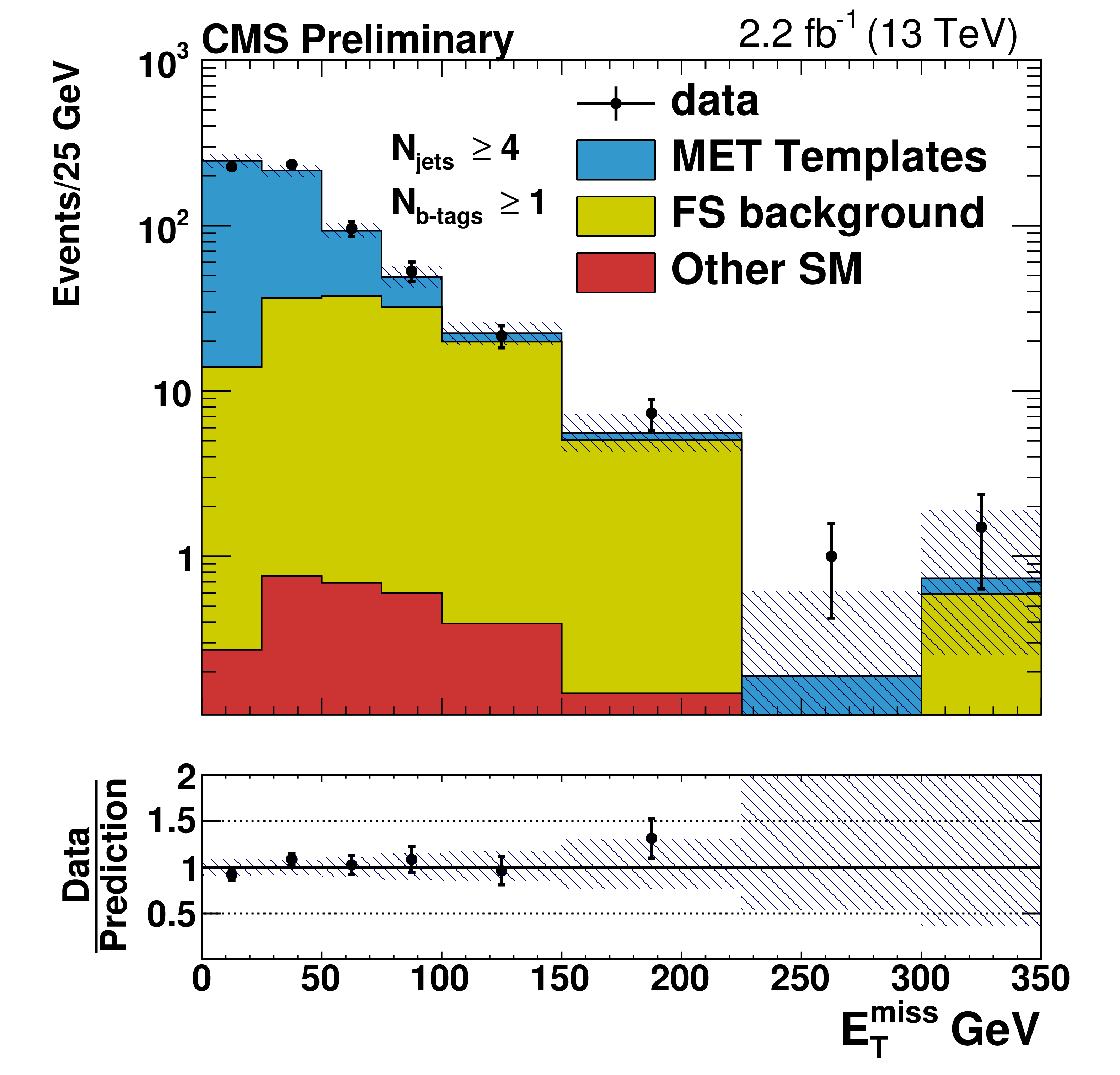
The $ {E_{\mathrm {T}}^{\text {miss}}} $ distribution is shown for data and the data-driven predictions in the on-Z signal regions. The top plots show the results in SRA where the left plot shows events with exactly 0 b-tagged jets, and the right plot shows events with $\geq $ 1 b-tagged jet. The second row of plots shows the results in SRB with the same b-tagging requirement as in the first row, and the bottom row shows the results in the ATLAS-like signal region. The ``Other SM'' category includes WZ, ZZ, and other rare SM backgrounds taken from MC. See Table XXX for yields. |

png ; pdf ; |
Figure 2-b:
The $ {E_{\mathrm {T}}^{\text {miss}}} $ distribution is shown for data and the data-driven predictions in the on-Z signal regions. The top plots show the results in SRA where the left plot shows events with exactly 0 b-tagged jets, and the right plot shows events with $\geq $ 1 b-tagged jet. The second row of plots shows the results in SRB with the same b-tagging requirement as in the first row, and the bottom row shows the results in the ATLAS-like signal region. The ``Other SM'' category includes WZ, ZZ, and other rare SM backgrounds taken from MC. See Table XXX for yields. |
png ; pdf ; |
Figure 2-c:
The $ {E_{\mathrm {T}}^{\text {miss}}} $ distribution is shown for data and the data-driven predictions in the on-Z signal regions. The top plots show the results in SRA where the left plot shows events with exactly 0 b-tagged jets, and the right plot shows events with $\geq $ 1 b-tagged jet. The second row of plots shows the results in SRB with the same b-tagging requirement as in the first row, and the bottom row shows the results in the ATLAS-like signal region. The ``Other SM'' category includes WZ, ZZ, and other rare SM backgrounds taken from MC. See Table XXX for yields. |
png ; pdf ; |
Figure 2-d:
The $ {E_{\mathrm {T}}^{\text {miss}}} $ distribution is shown for data and the data-driven predictions in the on-Z signal regions. The top plots show the results in SRA where the left plot shows events with exactly 0 b-tagged jets, and the right plot shows events with $\geq $ 1 b-tagged jet. The second row of plots shows the results in SRB with the same b-tagging requirement as in the first row, and the bottom row shows the results in the ATLAS-like signal region. The ``Other SM'' category includes WZ, ZZ, and other rare SM backgrounds taken from MC. See Table XXX for yields. |
png ; pdf ; |
Figure 2-e:
The $ {E_{\mathrm {T}}^{\text {miss}}} $ distribution is shown for data and the data-driven predictions in the on-Z signal regions. The top plots show the results in SRA where the left plot shows events with exactly 0 b-tagged jets, and the right plot shows events with $\geq $ 1 b-tagged jet. The second row of plots shows the results in SRB with the same b-tagging requirement as in the first row, and the bottom row shows the results in the ATLAS-like signal region. The ``Other SM'' category includes WZ, ZZ, and other rare SM backgrounds taken from MC. See Table XXX for yields. |

png ; pdf ; |
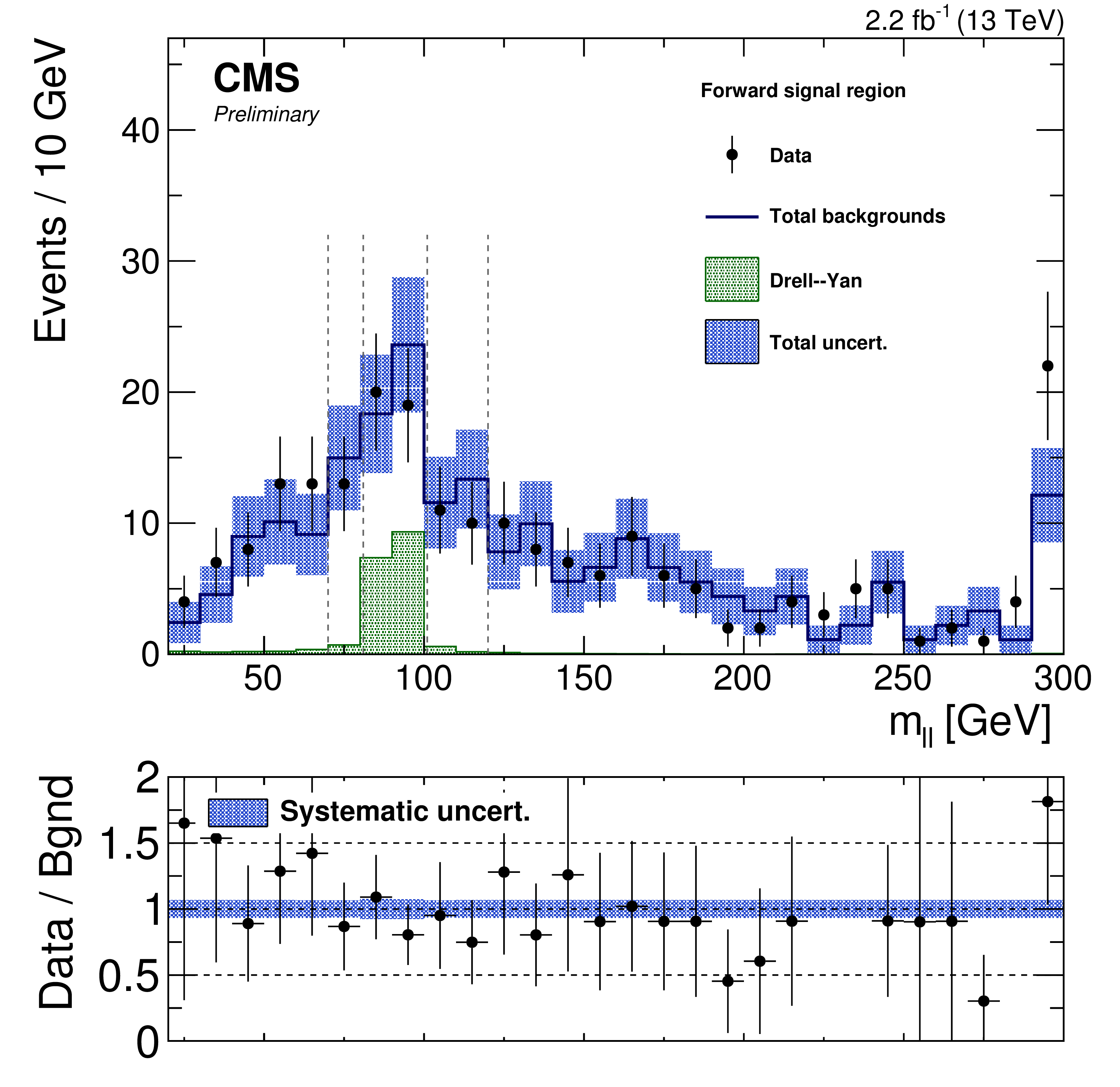
Figure 3-a:
The $m_{\ell \ell }$ spectra without requirements on b-tagged jets (top), for exactly zero b-tagged jets (middle) and at least one b-tagged jet (bottom) for central leptons (left) and forward leptons (right). The data is shown as black points, while the total background estimate and its uncertainty are shown as a solid blue line surrounded by a shaded blue band. The Drell-Yan background is shown as a shaded green area. |

png ; pdf ; |
Figure 3-b:
The $m_{\ell \ell }$ spectra without requirements on b-tagged jets (top), for exactly zero b-tagged jets (middle) and at least one b-tagged jet (bottom) for central leptons (left) and forward leptons (right). The data is shown as black points, while the total background estimate and its uncertainty are shown as a solid blue line surrounded by a shaded blue band. The Drell-Yan background is shown as a shaded green area. |

png ; pdf ; |
Figure 3-c:
The $m_{\ell \ell }$ spectra without requirements on b-tagged jets (top), for exactly zero b-tagged jets (middle) and at least one b-tagged jet (bottom) for central leptons (left) and forward leptons (right). The data is shown as black points, while the total background estimate and its uncertainty are shown as a solid blue line surrounded by a shaded blue band. The Drell-Yan background is shown as a shaded green area. |
png ; pdf ; |
Figure 3-d:
The $m_{\ell \ell }$ spectra without requirements on b-tagged jets (top), for exactly zero b-tagged jets (middle) and at least one b-tagged jet (bottom) for central leptons (left) and forward leptons (right). The data is shown as black points, while the total background estimate and its uncertainty are shown as a solid blue line surrounded by a shaded blue band. The Drell-Yan background is shown as a shaded green area. |

png ; pdf ; |
Figure 3-e:
The $m_{\ell \ell }$ spectra without requirements on b-tagged jets (top), for exactly zero b-tagged jets (middle) and at least one b-tagged jet (bottom) for central leptons (left) and forward leptons (right). The data is shown as black points, while the total background estimate and its uncertainty are shown as a solid blue line surrounded by a shaded blue band. The Drell-Yan background is shown as a shaded green area. |

png ; pdf ; |
Figure 3-f:
The $m_{\ell \ell }$ spectra without requirements on b-tagged jets (top), for exactly zero b-tagged jets (middle) and at least one b-tagged jet (bottom) for central leptons (left) and forward leptons (right). The data is shown as black points, while the total background estimate and its uncertainty are shown as a solid blue line surrounded by a shaded blue band. The Drell-Yan background is shown as a shaded green area. |
png ; pdf ; |
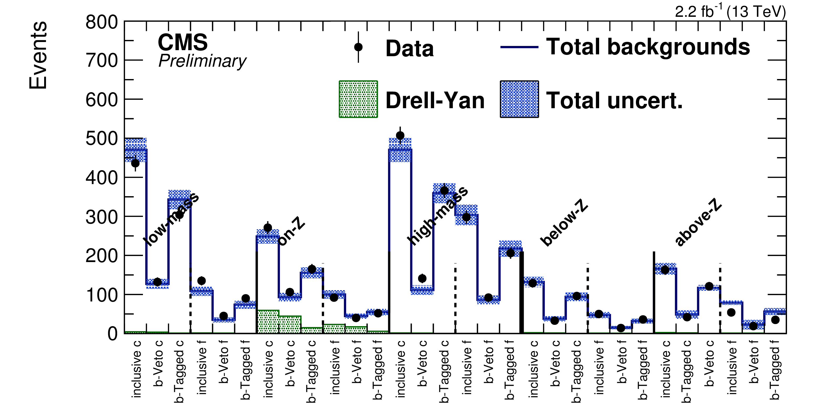
Figure 4-a:
Overview of results in all signal regions of both the edge (a) and the on-Z search (b). The data points in blue are compared to the background expectation, which is shown as a solid blue line, together with its uncertainty, shown as a blue band. For the edge search, the Drell-Yan backgrounds are shown as a shaded green area. |

png ; pdf ; |
Figure 4-b:
Overview of results in all signal regions of both the edge (a) and the on-Z search (b). The data points in blue are compared to the background expectation, which is shown as a solid blue line, together with its uncertainty, shown as a blue band. For the edge search, the Drell-Yan backgrounds are shown as a shaded green area. |

png ; pdf ; |
Figure 5:
Exclusion contours are shown when we interpret the results of this analysis in the GMSB model. The region to the left of the red (black) dotted line shows the masses which are excluded by the expected (observed) limit. |
png ; pdf ; |
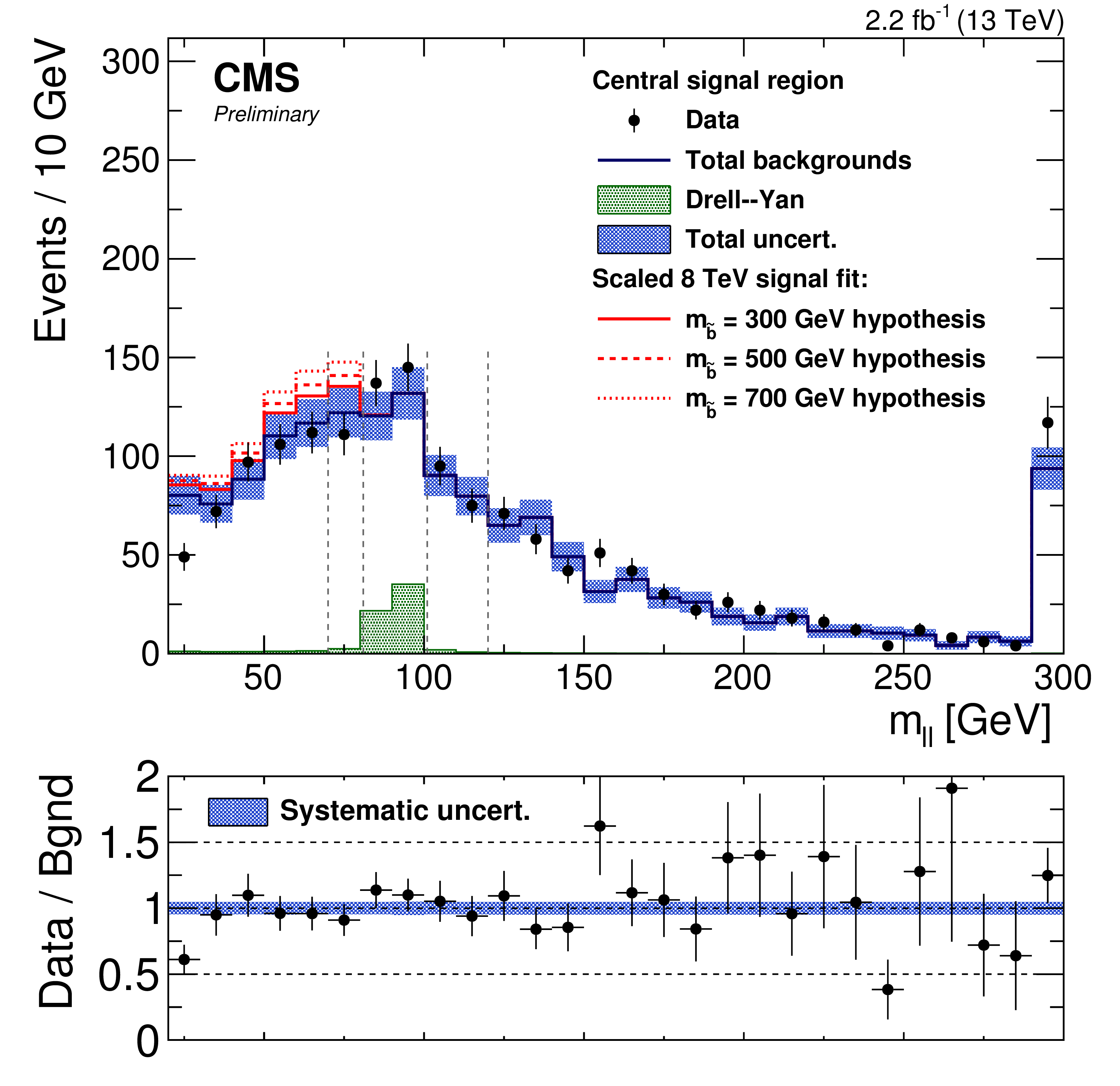
Figure 6:
The di-lepton invariant mass spectra for central leptons. The data is shown as black points, while the total background estimate and its uncertainty are shown as a solid blue line surrounded by a shaded blue band. The Drell-Yan background is shown as a shaded green area. The signal shape measured by CMS with 8 TeV data has been overlaid on top of the background prediction and has been normalized to the size of the excess observed at 8 TeV scaled by the ratio of integrated luminosity and cross sections for 3 different sbottom mass hypothesis. |
|
|
Compact Muon Solenoid LHC, CERN |
|

|

|

|

|

|