Mean Energy Loss

Energy loss processes are very similar for \(e^+/e^-\), \(\mu^+/\mu^-\) and charged hadrons, so a common description for them was a natural choice in Geant4 [eal03], [eal09]. Any energy loss process must calculate the continuous and discrete energy loss in a material. Below a given energy threshold the energy loss is continuous and above it the energy loss is simulated by the explicit production of secondary particles - gammas, electrons, and positrons.

Method

Let

\[\frac{d\sigma(Z,E,T)}{dT}\]

be the differential cross-section per atom (atomic number \(Z\)) for the ejection of a secondary particle with kinetic energy \(T\) by an incident particle of total energy \(E\) moving in a material of density \(\rho\). The value of the kinetic energy cut-off or production threshold is denoted by \(T_{cut}\). Below this threshold the soft secondaries ejected are simulated as continuous energy loss by the incident particle, and above it they are explicitly generated. The mean rate of energy loss is given by:

(29)\[\frac{dE_{soft}(E,T_{cut})}{dx} = n_{at} \cdot \int_{0}^{T_{cut}} \frac{d \sigma (Z,E,T)}{dT} T \: dT\]

where \(n_{at}\) is the number of atoms per volume in the material. The total cross section per atom for the ejection of a secondary of energy \(T > T_{cut}\) is

(30)\[\sigma (Z,E,T_{cut}) = \int_{T_{cut}}^{T_{max}}\frac{d \sigma (Z,E,T)} {dT} \: dT \,\]

where \(T_{max}\) is the maximum energy transferable to the secondary particle.

If there are several processes providing energy loss for a given particle, then the total continuous part of the energy loss is the sum:

(31)\[\frac{dE_{soft}^{tot}(E,T_{cut})}{dx} = \sum_i{\frac{dE_{soft,i}(E,T_{cut})}{dx}}.\]

These values are pre-calculated during the initialization phase of Geant4 and stored in the \(dE/dx\) table. Using this table the ranges of the particle in given materials are calculated and stored in the Range table. The Range table is then inverted to provide the InverseRange table. At run time, values of the particle’s continuous energy loss and range are obtained using these tables. Concrete processes contributing to the energy loss are not involved in the calculation at that moment. In contrast, the production of secondaries with kinetic energies above the production threshold is sampled by each concrete energy loss process.

The default energy interval for these tables extends from 100 eV to 100 TeV and the default number of bins is 84. For muons and for heavy particles energy loss processes models are valid for higher energies and can be extended. For muons the upper limit may be set to 1000 PeV.

General Interfaces

There are a number of similar functions for discrete electromagnetic processes and for electromagnetic (EM) packages an additional base classes were designed to provide common computations [eal09]. Common calculations for discrete EM processes are performed in the class G4VEnergyLossProcess. Derived classes (Table 13) are concrete processes providing initialisation. The physics models are implemented using the G4VEmModel interface. Each process may have one or many models defined to be active over a given energy range and set of G4Regions. Models are implementing computation of energy loss, cross section and sampling of final state. The list of EM processes and models for gamma incident is shown in Table 13.

Table 13 List of process and model classes for charged particles.

EM process	EM model	Ref.
G4eIonisation	G4MollerBhabhaModel	Ionisation
	G4LivermoreIonisationModel	Livermore Model
	G4PenelopeIonisationModel	Penelope Model
	G4PAIModel	Photoabsorption Ionisation Model
	G4PAIPhotModel	Photoabsorption Ionisation Model
G4ePolarizedIonisation	G4PolarizedMollerBhabhaModel	Ionisation
G4MuIonisation	G4MuBetheBlochModel	Muon Ionisation
	G4PAIModel	Photoabsorption Ionisation Model
	G4PAIPhotModel	Photoabsorption Ionisation Model
G4hIonisation	G4BetheBlochModel	Hadron and Ion Ionisation
	G4BraggModel	Hadron and Ion Ionisation
	G4ICRU73QOModel	Energy losses of slow negative particles
	G4PAIModel	Photoabsorption Ionisation Model
	G4PAIPhotModel	Photoabsorption Ionisation Model
G4ionIonisation	G4BetheBlochModel	Hadron and Ion Ionisation
	G4BetheBlochIonGasModel	Hadron and Ion Ionisation
	G4BraggIonModel	Hadron and Ion Ionisation
	G4BraggIonGasModel	Hadron and Ion Ionisation
	G4IonParametrisedLossModel	ICRU 73-based energy loss model
	G4AtimaEnergyLossModel	ATIMA energy-loss model
	G4LindhardSorensenIonModel
G4NuclearStopping	G4ICRU49NuclearStoppingModel	Nuclear Stopping
G4mplIonisation	G4mplIonisationWithDeltaModel
G4eBremsstrahlung	G4SeltzerBergerModel	Seltzer-Berger bremsstrahlung model
	G4eBremsstrahlungRelModel	Bremsstrahlung of high-energy electrons
	G4LivermoreBremsstrahlungModel	Livermore Model
	G4PenelopeBremsstrahlungModel	Penelope Model
G4ePolarizedBremsstrahlung	G4PolarizedBremsstrahlungModel	Polarized Bremsstrahlung for electron and positron
G4MuBremsstrahlung	G4MuBremsstrahlungModel	Bremsstrahlung
G4hBremsstrahlung	G4hBremsstrahlungModel	Bremsstrahlung
G4ePairProduction	G4MuPairProductionModel	Positron - Electron Pair Production by Muons
G4MuPairProduction	G4MuPairProductionModel	Positron - Electron Pair Production by Muons
G4hPairProduction	G4hPairProductionModel	Positron - Electron Pair Production by Muons

Step-size Limit

Continuous energy loss imposes a limit on the step-size because of the energy dependence of the cross sections. It is generally assumed in MC programs (for example, Geant3) that the cross sections are approximately constant along a step, i.e. the step size should be small enough, so that the change in cross section along the step is also small. In principle one must use very small steps in order to insure an accurate simulation, however the computing time increases as the step-size decreases.

For EM processes the exact solution is available (see Correcting the Cross Section for Energy Variation) but is is not implemented yet for all physics processes including hadronics. A good compromise is to limit the step-size by not allowing the stopping range of the particle to decrease by more than ~20% during the step. This condition works well for particles with kinetic energies >1 MeV, but for lower energies it gives too short step-sizes, so must be relaxed. To solve this problem a lower limit on the step-size was introduced. A smooth StepFunction, with 2 parameters, controls the step size. At high energy the maximum step size is defined by Step/Range \(\sim \alpha_R\) (parameter dRoverRange). By default \(\alpha_R = 0.2\). As the particle travels the maximum step size decreases gradually until the range becomes lower than \(\rho_R\) (parameter finalRange). Default finalRange \(\rho_R = 1\) mm. For the case of a particle range \(R > \rho_R\) the StepFunction provides limit for the step size \(\Delta S_{lim}\) by the following formula:

(32)\[\Delta S_{lim} = \alpha_R R + \rho_R (1- \alpha_R ) \left(2-\frac{\rho_R}{R} \right).\]

In the opposite case of a small range \(\Delta S_{lim} = R\). The figure below shows the ratio step/range as a function of range if step limitation is determined only by the expression (32).

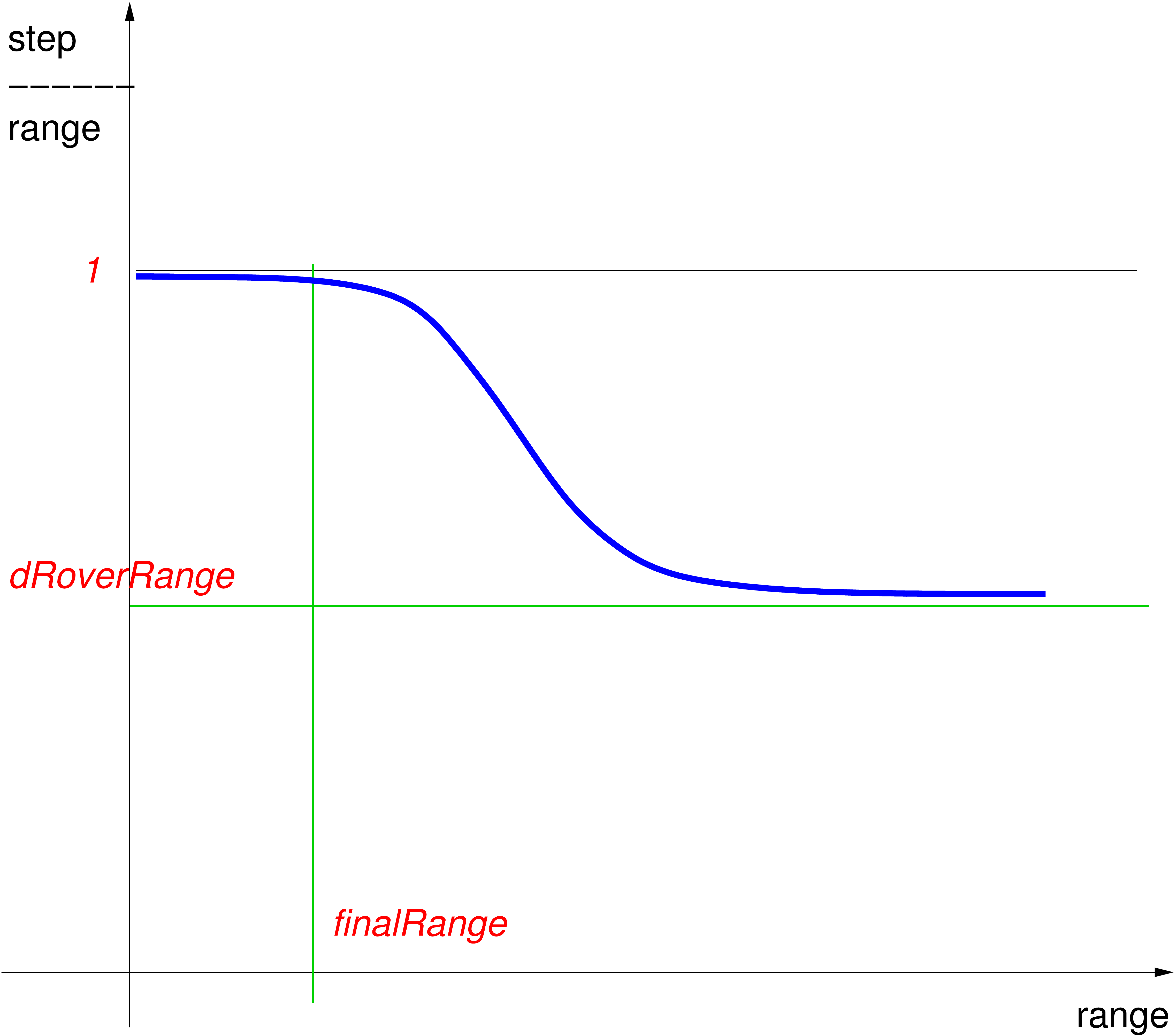
Fig. 17 Step limit.

The parameters of StepFunction can be overwritten using a UI command:

/process/eLoss/StepFunction 0.2 1 mm

To provide more accurate simulation of particle ranges in physics constructors G4EmStandardPhysics_option3 and G4EmStandardPhysics_option4 more strict step limitation is chosen for different particle types.

Run Time Energy Loss Computation

The computation of the mean energy loss after a given step is done by using the \(dE/dx\), Range, and InverseRange tables. The \(dE/dx\) table is used if the energy deposition (\(\Delta T\)) is less than allowed limit \(\Delta T < \xi T_0\), where \(\xi\) is \(linearLossLimit\) parameter (by default \(\xi = 0.01\)), \(T_0\) is the kinetic energy of the particle. In that case

\[\Delta T = \frac{dE}{dx}\Delta s,\]

where \(\Delta T\) is the energy loss, \(\Delta s\) is the true step length. When a larger percentage of energy is lost, the mean loss can be written as

\[\Delta T = T_0 - f_T(r_0- \Delta s)\]

where \(r_0\) the range at the beginning of the step, the function \(f_T(r)\) is the inverse of the Range table (i.e. it gives the kinetic energy of the particle for a range value of r. By default spline approximation is used to retrieve a value from \(dE/dx\), Range, and InverseRange tables. The spline flag can be changed using an UI command:

/process/em/spline false

After the mean energy loss has been calculated, the process computes the actual energy loss, i.e. the loss with fluctuations. The fluctuation models are described in Energy Loss Fluctuations.

If deexcitation module (see Atomic relaxation) is enabled then simulation of atomic deexcitation is performed using information on step length and ionisation cross section. Fluorescence gamma and Auger electrons are produced above the same threshold energy as \(\delta\)-electrons and bremsstrahlung gammas. The following UI commands can be used to enable atomic relaxation:

/process/em/deexcitation myregion true true true
/process/em/fluo true
/process/em/auger true
/process/em/pixe true
/process/em/deexcitationIgnoreCut true

The last command means that production threshold for electrons and gammas are not checked, so full atomic de-excitation decay chain is simulated.

After the step a kinetic energy of a charged particle is compared with the lowestEnergy. In the case if final kinetic energy is below the particle is stopped and remaining kinetic energy is assigned to the local energy deposit. The default value of the limit is 1 keV. It may be changed separately for electron/positron and muon/hadron using UI commands:

/process/em/lowestElectronEnergy 100 eV
/process/em/lowestMuHadEnergy 50 eV

These values may be set to zero.

Energy Loss by Heavy Charged Particles

To save memory in the case of positively charged hadrons and ions energy loss, \(dE/dx\), Range and InverseRange tables are constructed only for proton, antiproton, muons, pions, kaons, and Generic Ion. The energy loss for other particles is computed from these tables at the scaled kinetic energy \(T_{scaled}\):

(33)\[T_{scaled} = T\frac{ M_{base}}{ M_{particle}},\]

where T is the kinetic energy of the particle, \(M_{base}\) and \(M_{particle}\) are the masses of the base particle (proton or kaon) and particle. For positively changed hadrons with non-zero spin proton is used as a based particle, for negatively charged hadrons with non-zero spin - antiproton, for charged particles with zero spin - \(K^+\) or \(K^-\) correspondingly. The virtual particle Generic Ion is used as a base particle for for all ions with \(Z > 2\). It has mass, change and other quantum numbers of the proton. The energy loss can be defined via scaling relation:

\[\frac{dE}{dx}(T) = q^2_{eff}(F_1(T)\frac{dE}{dx}_{base}(T_{scaled}) + F_2(T,q_{eff})),\]

where \(q_{eff}\) is particle effective change in units of positron charge, \(F_1\) and \(F_2\) are correction function taking into account Birks effect, Block correction, low-energy corrections based on data from evaluated data bases [eal05]. For a hadron \(q_{eff}\) is equal to the hadron charge, for a slow ion effective charge is different from the charge of the ion’s nucleus, because of electron exchange between transporting ion and the media. The effective charge approach is used to describe this effect [ZM88]. The scaling relation (33) is valid for any combination of two heavy charged particles with accuracy corresponding to high order mass, charge and spin corrections [eal93].

Bibliography

eal09(1,2,3)

J. Apostolakis et al. Geometry and physics of the geant4 toolkit for high and medium energy applications. Radiation Physics and Chemistry, 78(10):859–873, oct 2009. URL: https://doi.org/10.1016/j.radphyschem.2009.04.026, doi:10.1016/j.radphyschem.2009.04.026.

eal93

M.J. Berger et al. Report 49. Journal of the International Commission on Radiation Units and Measurements, os25(2):NP–NP, may 1993. ICRU Report 49. URL: https://doi.org/10.1093/jicru/os25.2.Report49, doi:10.1093/jicru/os25.2.report49.

eal05

P. Sigmund et al. Stopping of ions heavier than helium. Journal of the International Commission on Radiation Units and Measurements, jun 2005. ICRU Report 73. URL: https://doi.org/10.1093/jicru/ndi001, doi:10.1093/jicru/ndi001.

eal03

S. Agostinelli et al. Geant4—a simulation toolkit. Nucl. Instr. and Meth. in Phys. Research Section A, 506(3):250–303, jul 2003. URL: https://doi.org/10.1016/S0168-9002(03)01368-8, doi:10.1016/s0168-9002(03)01368-8.

ZM88

J.F. Ziegler and J.M. Manoyan. Nucl. Instr. and Meth. B, 35():215, 1988.