Introduction

With the EM polarization extension it is possible to track polarized particles (leptons and photons). Special emphasis will be put in the proper treatment of polarized matter and its interaction with longitudinal polarized electrons/positrons or circularly polarized photons, which is for instance essential for the simulation of positron polarimetry. The implementation is base on Stokes vectors [McM61]. Further details can be found in [Lai08].

In its current state, the following polarization dependent processes are considered:

• Bhabha/Møller scattering,

• Positron Annihilation,

• Compton scattering,

• Pair creation,

• Bremsstrahlung.

Several simulation packages for the realistic description of the development of electromagnetic showers in matter have been developed. A prominent example of such codes is EGS (Electron Gamma Shower) [NHR85]. For this simulation framework extensions with the treatment of polarized particles exist [Flottmann93a][NBH93][LKNS]; the most complete has been developed by K. Flöttmann [Flottmann93a]. It is based on the matrix formalism [McM61], which enables a very general treatment of polarization. However, the Flöttmann extension concentrates on evaluation of polarization transfer, i.e. the effects of polarization induced asymmetries are neglected, and interactions with polarized media are not considered.

Another important simulation tool for detector studies is Geant3 [eal85]. Here also some effort has been made to include polarization [aal][Hoo97], but these extensions are not publicly available.

In general the implementation of polarization in this EM polarization library follows very closely the approach by K. Flöttmann [Flottmann93a]. The basic principle is to associate a Stokes vector to each particle and track the mean polarization from one interaction to another. The basics for this approach is the matrix formalism as introduced in [McM61].

Stokes vector

The Stokes vector [Sto52][McM61] is a rather simple object (in comparison to e.g. the spin density matrix), three real numbers are sufficient for the characterization of the polarization state of any single electron, positron or photon. Using Stokes vectors all possible polarization states can be described, i.e. circular and linear polarized photons can be handled with the same formalism as longitudinal and transverse polarized electron/positrons.

The Stokes vector can be used also for beams, in the sense that it defines a mean polarization.

In the EM polarization library the Stokes vector is defined as follows:

	Photons	Electrons
\(\xi_1\)	linear polarization	polarization in x direction
\(\xi_2\)	linear polarization but \(\pi/4\) to right	polarization in y direction
\(\xi_3\)	circular polarization	polarization in z direction

This definition is assumed in the particle reference frame, i.e. with the momentum of the particle pointing to the z direction, cf. also next section about coordinate transformations. Correspondingly a 100% longitudinally polarized electron or positron is characterized by

\[\begin{split}{{\boldsymbol{\xi}}}=\mbox{$\scriptscriptstyle\left(\begin{array}{c}0\\0\\\pm1\end{array}\right)$},\end{split}\]

where \(\pm1\) corresponds to spin parallel (anti parallel) to particle’s momentum. Note that this definition is similar, but not identical to the definition used in McMaster [McM61].

Many scattering cross sections of polarized processes using Stokes vectors for the characterization of initial and final states are available in [McM61]. In general a differential cross section has the form

\[\frac{d\sigma({{\boldsymbol{\zeta}}}^{(1)},{{\boldsymbol{\zeta}}}^{(2)},{{\boldsymbol{\xi}}}^{(1)},{{\boldsymbol{\xi}}}^{(2)})}{d\Omega}\;,\]

i.e. it is a function of the polarization states of the initial particles \({{\boldsymbol{\zeta}}}^{(1)}\) and \({{\boldsymbol{\zeta}}}^{(2)}\), as well as of the polarization states of the final state particles \({{\boldsymbol{\xi}}}^{(1)}\) and \({{\boldsymbol{\xi}}}^{(2)}\) (in addition to the kinematic variables \(E\), \(\theta\), and \(\phi\)).

Consequently, in a simulation we have to account for

• Asymmetries:

• Polarization of beam (\({{\boldsymbol{\zeta}}}^{(1)}\)) and target (\({{\boldsymbol{\zeta}}}^{(2)}\)) can induce azimuthal and polar asymmetries, and may also influence on the total cross section (Geant4: GetMeanFreePath()).

• Polarization transfer / depolarization effects

• The dependence on the final state polarizations defines a possible transfer from initial polarization to final state particles.

Transfer matrix

Using the formalism of McMaster, differential cross section and polarization transfer from the initial state (\({{\boldsymbol{\zeta}}}^{(1)}\)) to one final state particle (\({{\boldsymbol{\xi}}}^{(1)}\)) are combined in an interaction matrix \(T\):

\[\begin{split}\left(\begin{array}{c} O \\ {{\boldsymbol{\xi}}}^{(1)} \end{array}\right) = T \, \left(\begin{array}{c} I \\ {{\boldsymbol{\zeta}}}^{(1)} \end{array}\right)\;,\end{split}\]

where \(I\) and \(O\) are the incoming and outgoing currents, respectively. In general the \(4\times4\) matrix \(T\) depends on the target polarization \({{\boldsymbol{\zeta}}}^{(2)}\) (and of course on the kinematic variables \(E\), \(\theta\), \(\phi\)). Similarly one can define a matrix defining the polarization transfer to second final state particle like

\[\begin{split}\left(\begin{array}{c} O \\ {{\boldsymbol{\xi}}}^{(2)} \end{array}\right) = T' \, \left(\begin{array}{c}I\\ {{\boldsymbol{\zeta}}}^{(1)}\end{array}\right) \;.\end{split}\]

In this framework the transfer matrix \(T\) is of the form

\[\begin{split}T = \left( \begin{array}{llll} S & A_1 & A_2 & A_3 \\ P_1 & M_{11} & M_{21} & M_{31} \\ P_2 & M_{12} & M_{22} & M_{32} \\ P_3 & M_{13} & M_{23} & M_{33} \\ \end{array} \right) \;.\end{split}\]

The matrix elements \(T_{ij}\) can be identified as (unpolarized) differential cross section (\(S\)), polarized differential cross section (\(A_j\)), polarization transfer (\(M_{ij}\)), and (de)polarization (\(P_i\)). In the Flöttmann extension the elements \(A_j\) and \(P_i\) have been neglected, thus concentrating on polarization transfer only. Using the full matrix takes now all polarization effects into account.

The transformation matrix, i.e. the dependence of the mean polarization of final state particles, can be derived from the asymmetry of the differential cross section w.r.t. this particular polarization. Where the asymmetry is defined as usual by

\[A = \frac{\sigma(+1)-\sigma(-1)}{\sigma(+1)+\sigma(-1)} \;.\]

The mean final state polarizations can be determined coefficient by coefficient. In general, the differential cross section is a linear function of the polarizations, i.e.

\[\frac{d\sigma({{\boldsymbol{\zeta}}}^{(1)},{{\boldsymbol{\zeta}}}^{(2)},{{\boldsymbol{\xi}}}^{(1)},{{\boldsymbol{\xi}}}^{(2)})}{d\Omega} = \Phi_{(\zeta^{(1)},\zeta^{(2)})} + {{\boldsymbol{A}}}_{(\zeta^{(1)},\zeta^{(2)})} \cdot{{\boldsymbol{\xi}}}^{(1)} + {{\boldsymbol{B}}}_{(\zeta^{(1)},\zeta^{(2)})} \cdot{{\boldsymbol{\xi}}}^{(2)} + {{{\boldsymbol{\xi}}}^{(1)}}^T M_{(\zeta^{(1)},\zeta^{(2)})} \,{{\boldsymbol{\xi}}}^{(2)}\]

In this form, the mean polarization of the final state can be read off easily, and one obtains

\[\begin{split}\langle{{\boldsymbol{\xi}}}^{(1)}\rangle &= \frac{1}{\Phi_{(\zeta^{(1)},\zeta^{(2)})}} {{\boldsymbol{A}}}_{(\zeta^{(1)},\zeta^{(2)})} \;\; \mbox{and} \\ \langle{{\boldsymbol{\xi}}}^{(2)}\rangle &= \frac{1}{\Phi_{(\zeta^{(1)},\zeta^{(2)})}} {{\boldsymbol{B}}}_{(\zeta^{(1)},\zeta^{(2)})} \;.\end{split}\]

Note that the mean polarization states do not depend on the correlation matrix \(M_{(\zeta^{(1)},\zeta^{(2)})}\). In order to account for correlation one has to generate single particle Stokes vector explicitly, i.e. on an event by event basis. However, this implementation generates mean polarization states, and neglects correlation effects.

Coordinate transformations

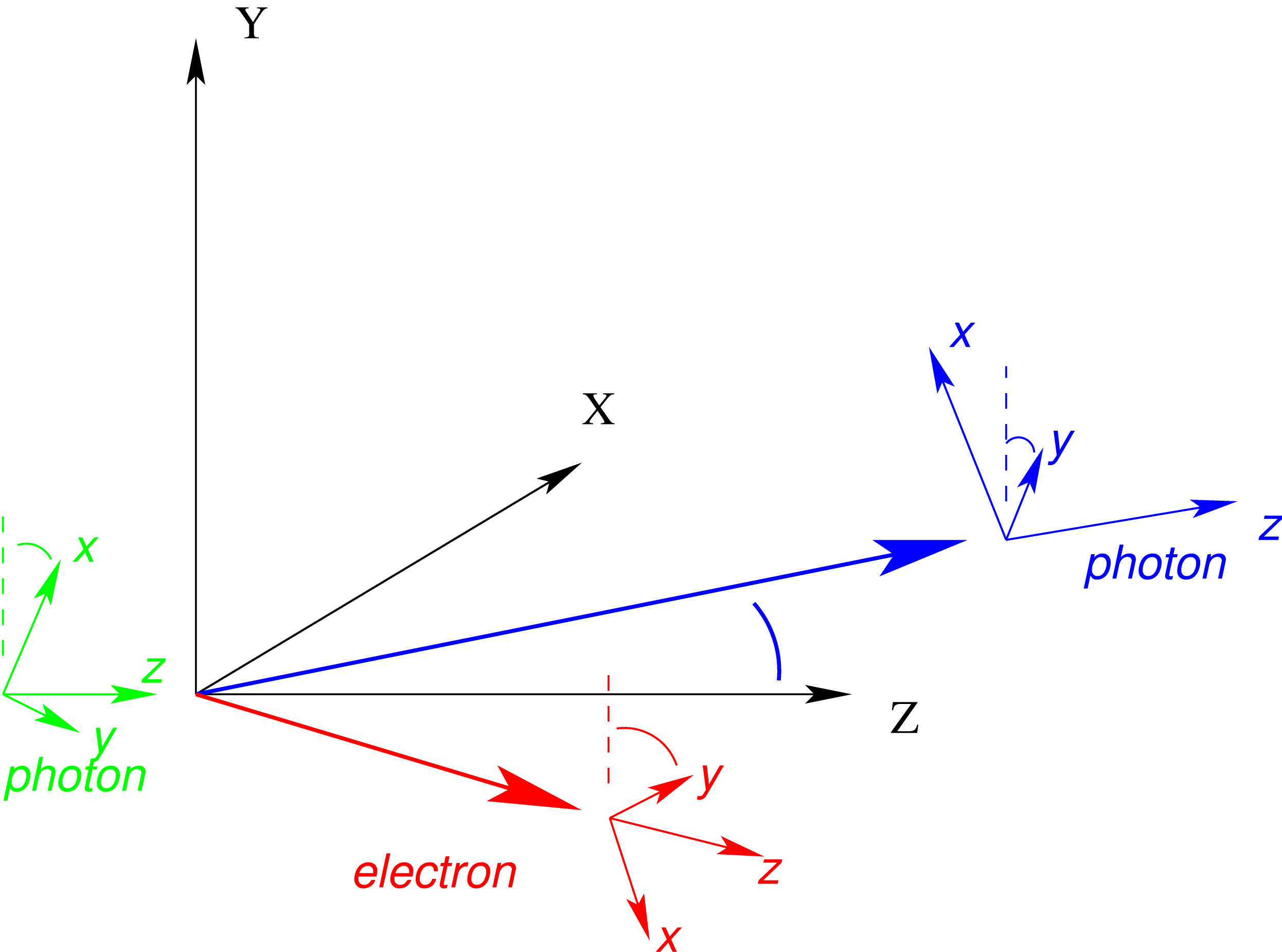
Fig. 32 The interaction frame and the particle frames for the example of Compton scattering. The momenta of all participating particle lie in the \(x\)-\(z\)-plane, the scattering plane. The incoming photon gives the \(z\) direction. The outgoing photon is defined as particle 1 and gives the \(x\)-direction, perpendicular to the \(z\)-axis. The \(y\)-axis is then perpendicular to the scattering plane and completes the definition of a right handed coordinate system called interaction frame. The particle frame is defined by the Geant4 routine G4ThreeMomemtum::rotateUz().

Three different coordinate systems are used in the evaluation of polarization states:

• World frame The geometry of the target, and the momenta of all particles in Geant4 are noted in the world frame \(X\), \(Y\), \(Z\) (the global reference frame, GRF). It is the basis of the calculation of any other coordinate system.

• Particle frame Each particle is carrying its own coordinate system. In this system the direction of motion coincides with the \(z\)-direction. Geant4 provides a transformation from any particle frame to the World frame by the method G4ThreeMomemtum::rotateUz(). Thus, the \(y\)-axis of the particle reference frame (PRF) lies in the \(X\)-\(Y\)-plane of the world frame.

  The Stokes vector of any moving particle is defined w.r.t. the corresponding particle frame. Particles at rest (e.g. electrons of a media) use the world frame as particle frame.

• Interaction frame For the evaluation of the polarization transfer another coordinate system is used, defined by the scattering plane, cf. Fig. 32. There the \(z\)-axis is defined by the direction of motion of the incoming particle. The scattering plane is spanned by the \(z\)-axis and the \(x\)-axis, in a way, that the direction of particle 1 has a positive \(x\) component. The definition of particle 1 depends on the process, for instance in Compton scattering, the outgoing photon is referred as particle 11.

All frames are right handed.

Polarized beam and material

Polarization of beam particles is well established. It can be used for simulating low-energy Compton scattering of linear polarized photons. The interpretation as Stokes vector allows now the usage in a more general framework. The polarization state of a (initial) beam particle can be fixed using the standard ParticleGunMessenger class. For example, the class G4ParticleGun provides the method SetParticlePolarization(), which is usually accessible via:

/gun/polarization <Sx> <Sy> <Sz>

in a macro file.

In addition for the simulation of polarized media, a possibility to assign Stokes vectors to physical volumes is provided by a new class, the so-called G4PolarizationManager. The procedure to assign a polarization vector to a media, is done during the detector construction. There the logical volumes with certain polarization are made known to polarization manager. One example DetectorConstruction might look like follows:

G4double Targetthickness = .010*mm;
G4double Targetradius    = 2.5*mm;

G4Tubs* solidTarget =
  new G4Tubs("solidTarget",
             0.0,
             Targetradius,
             Targetthickness/2,
             0.0*deg,
             360.0*deg );

G4LogicalVolume * logicalTarget =
  new G4LogicalVolume(solidTarget,
                      iron,
                      "logicalTarget",
                      0,0,0);

G4VPhysicalVolume *  physicalTarget =
  new G4PVPlacement(0,G4ThreeVector(0.*mm, 0.*mm, 0.*mm),
                    logicalTarget,
                    "physicalTarget",
                    worldLogical,
                    false,
                    0);

G4PolarizationManager * polMgr = G4PolarizationManager::GetInstance();
polMgr->SetVolumePolarization(logicalTarget,G4ThreeVector(0.,0.,0.08));

Once a logical volume is known to the G4PolarizationManager, its polarization vector can be accessed from a macro file by its name, e.g. the polarization of the logical volume called “logicalTarget” can be changed via:

/polarization/volume/set logicalTarget 0. 0. -0.08

Note, the polarization of a material is stated in the world frame.

Ionisation

Method

The class G4ePolarizedIonization provides continuous and discrete energy losses of polarized electrons and positrons in a material. It evaluates polarization transfer and – if the material is polarized – asymmetries in the explicit delta rays production. The implementation baseline follows the approach derived for the class G4eIonization described in Mean Energy Loss and Ionisation. For continuous energy losses the effects of a polarized beam or target are negligible provided the separation cut \(T_{\rm cut}\) is small, and are therefore not considered separately. On the other hand, in the explicit production of delta rays by Møller or Bhabha scattering, the effects of polarization on total cross section and mean free path, on distribution of final state particles and the average polarization of final state particles are taken into account.

Total cross section and mean free path

Kinematics of Bhabha and Møller scattering is fixed by initial energy

\[\gamma=\frac{E_{k_1}}{m c^2}\]

and variable

\[\epsilon = \frac{E_{p_2}-m c^2}{E_{k_1}-m c^2},\]

which is the part of kinetic energy of initial particle carried out by scatter. Lower kinematic limit for \(\epsilon\) is \(0\), but in order to avoid divergences in both total and differential cross sections one sets

\[\epsilon_{min}= x = \frac{T_{min}}{E_{k_1}-mc^2},\]

where \(T_{min}\) has meaning of minimal kinetic energy of secondary electron. And, \(\epsilon_{\rm max}=1(1/2)\) for Bhabha(Møller) scatterings.

Total Møller cross section

The total cross section of the polarized Møller scattering can be expressed as follows

\[\sigma^M_{pol}=\frac{2\pi\gamma^2 r_e^2}{(\gamma-1)^2(\gamma+1)}\left[ \sigma^M_0 + \zeta_3^{(1)}\zeta_3^{(2)}\sigma^M_L + \left(\zeta_1^{(1)}\zeta_1^{(2)}+\zeta_2^{(1)}\zeta_2^{(2)}\right)\sigma^M_T\right],\]

where the \(r_e\) is classical electron radius, and

\[\begin{split}\sigma^M_0 &= - \frac{1}{1 - x} + \frac{1}{x} - \frac{{\left( \gamma - 1 \right)}^2}{{\gamma}^2} \left(\frac{1}{2} - x \right) + \frac{ 2 - 4\,\gamma }{2\,{\gamma}^2} \,\ln \left(\frac{1-x}{x}\right) \\ \sigma^M_L &= \frac{ \left( -3 + 2\,\gamma + {\gamma}^2 \right) \,\left( 1 - 2\,x \right) }{2\, {\gamma}^2} + \frac{2\,\gamma\,\left( -1 + 2\,\gamma \right)}{2\, {\gamma}^2} \,\ln \left(\frac{1-x}{x}\right) \\ \sigma^M_T &= \frac{2\,\left( \gamma - 1 \right) \,\left( 2\,x -1 \right)}{2\,{\gamma}^2} + \frac{ \left( 1 - 3\,\gamma \right) }{2\,{\gamma}^2} \,\ln \left(\frac{1-x}{x}\right)\end{split}\]

Total Bhabha cross section

The total cross section of the polarized Bhabha scattering can be expressed as follows

\[\sigma^B_{pol}=\frac{2\pi r_e^2}{\gamma-1} \left[ \sigma^B_0 + \zeta_3^{(1)}\zeta_3^{(2)}\sigma^B_L + \left(\zeta_1^{(1)}\zeta_1^{(2)} + \zeta_2^{(1)}\zeta_2^{(2)}\right)\sigma^B_T \right],\]

where

\[\begin{split}\sigma^B_0 &= \frac{1 - x}{2\,\left( \gamma - 1 \right) \,x} + \frac{2\,\left( -1 + 3\,x - 6\,x^2 + 4\,x^3 \right) } {3\,{\left( 1 + \gamma \right) }^3} \\ &+ \frac{-1 - 5\,x + 12\,x^2 - 10\,x^3 + 4\,x^4}{2\,\left( 1 + \gamma \right) \,x} + \frac{-3 - x + 8\,x^2 - 4\,x^3 - \ln (x)}{{\left( 1 + \gamma \right) }^2} \\ &+ \frac{3 + 4\,x - 9\,x^2 + 3\,x^3 - x^4 + 6\,x\,\ln (x)}{3\,x} \\ \sigma^B_L &= \frac{2\,\left( 1 - 3\,x + 6\,x^2 - 4\,x^3 \right) }{3\,{\left( 1 + \gamma \right) }^3} + \frac{-14 + 15\,x - 3\,x^2 + 2\,x^3 - 9\,\ln (x)}{3\,\left( 1 + \gamma \right) } \\ &+ \frac{5 + 3\,x - 12\,x^2 + 4\,x^3 + 3\,\ln (x)}{3\,{\left( 1 + \gamma \right) }^2} + \frac{7 - 9\,x + 3\,x^2 - x^3 + 6\,\ln (x)}{3} \\ \sigma^B_T &= \frac{2\,\left( -1 + 3\,x - 6\,x^2 + 4\,x^3 \right) }{3\,{\left( 1 + \gamma \right) }^3} + \frac{-7 - 3\,x + 18\,x^2 - 8\,x^3 - 3\,\ln (x)}{3\,{\left( 1 + \gamma \right) }^2} \\ &+ \frac{5 + 3\,x - 12\,x^2 + 4\,x^3 + 9\,\ln (x)}{6\,\left( 1 + \gamma \right) }\end{split}\]

Mean free path

With the help of the total polarized Møller cross section one can define a longitudinal asymmetry \(A^M_L\) and the transverse asymmetry \(A^M_T\), by

\[A^M_L = \displaystyle \frac{\sigma^M_L}{\sigma^M_0}\]

and

\[\quad A^M_T = \displaystyle \frac{\sigma^M_T}{\sigma^M_0} .\]

Similarly, using the polarized Bhabha cross section one can introduce a longitudinal asymmetry \(A^B_L\) and the transverse asymmetry \(A^B_T\) via

\[A^B_L = \displaystyle \frac{\sigma^B_L}{\sigma^B_0}\]

and

\[A^B_T = \displaystyle \frac{\sigma^B_T}{\sigma^B_0}\]

These asymmetries are depicted in Fig. 33, Fig. 34 for Møller and Fig. 35, Fig. 36 for Bhabha.

If both beam and target are polarized the mean free path as defined in Ionisation has to be modified. In the class G4ePolarizedIonization the polarized mean free path \(\lambda^{\rm pol}\) is derived from the unpolarized mean free path \(\lambda^{\rm unpol}\) via

\[\lambda^{\rm pol} = \frac{\lambda^{\rm unpol}}{1 + \zeta_3^{(1)}\zeta_3^{(2)}\, A_L + \left(\zeta_1^{(1)}\zeta_1^{(2)}+\zeta_2^{(1)}\zeta_2^{(2)}\right) \,A_T}\]

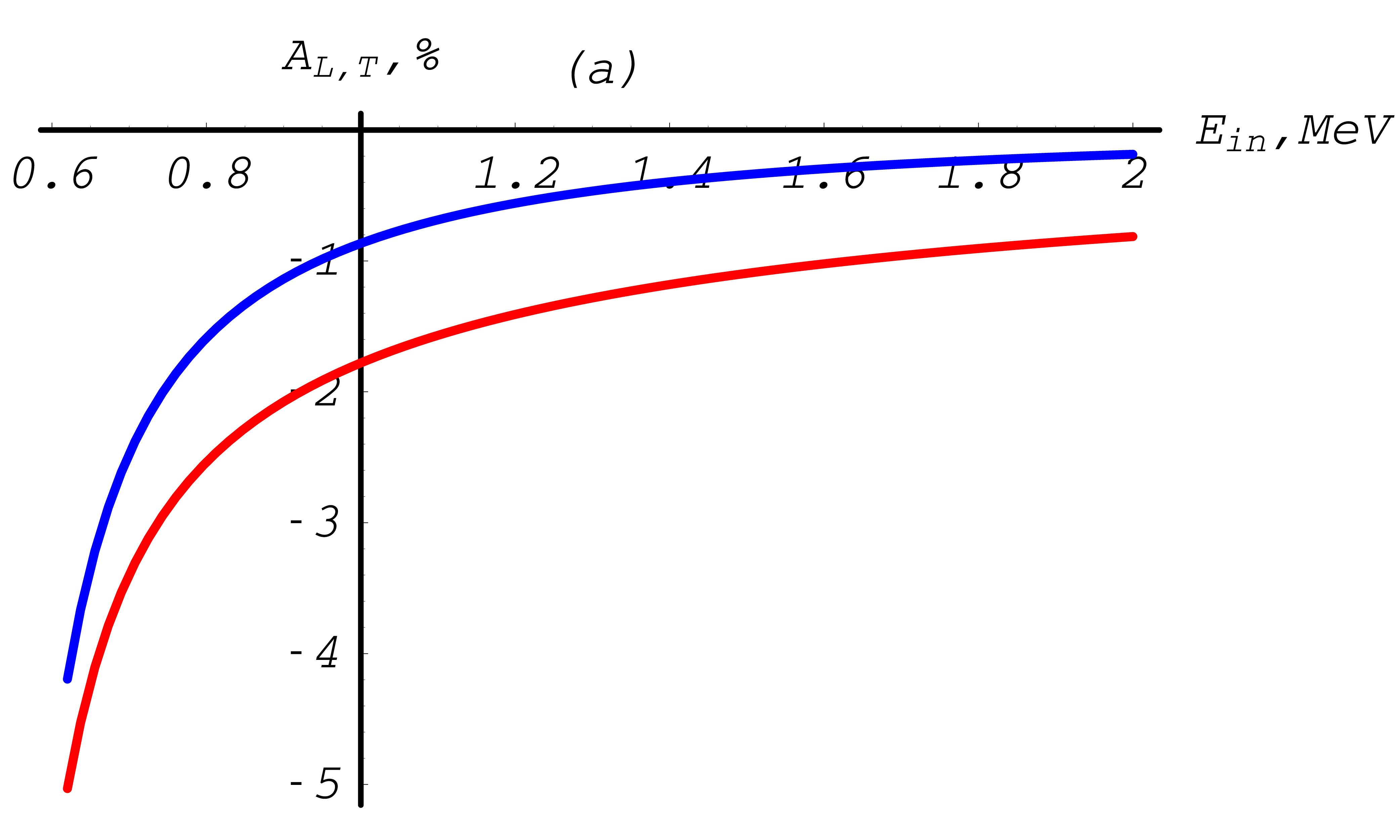
Fig. 33 Møller total cross section asymmetries depending on the total energy of the incoming electron, with a cut-off \(T_{\rm cut}= 1\) keV. Transverse asymmetry is plotted in blue, longitudinal asymmetry in red. Between 0.5 MeV and 2 MeV.

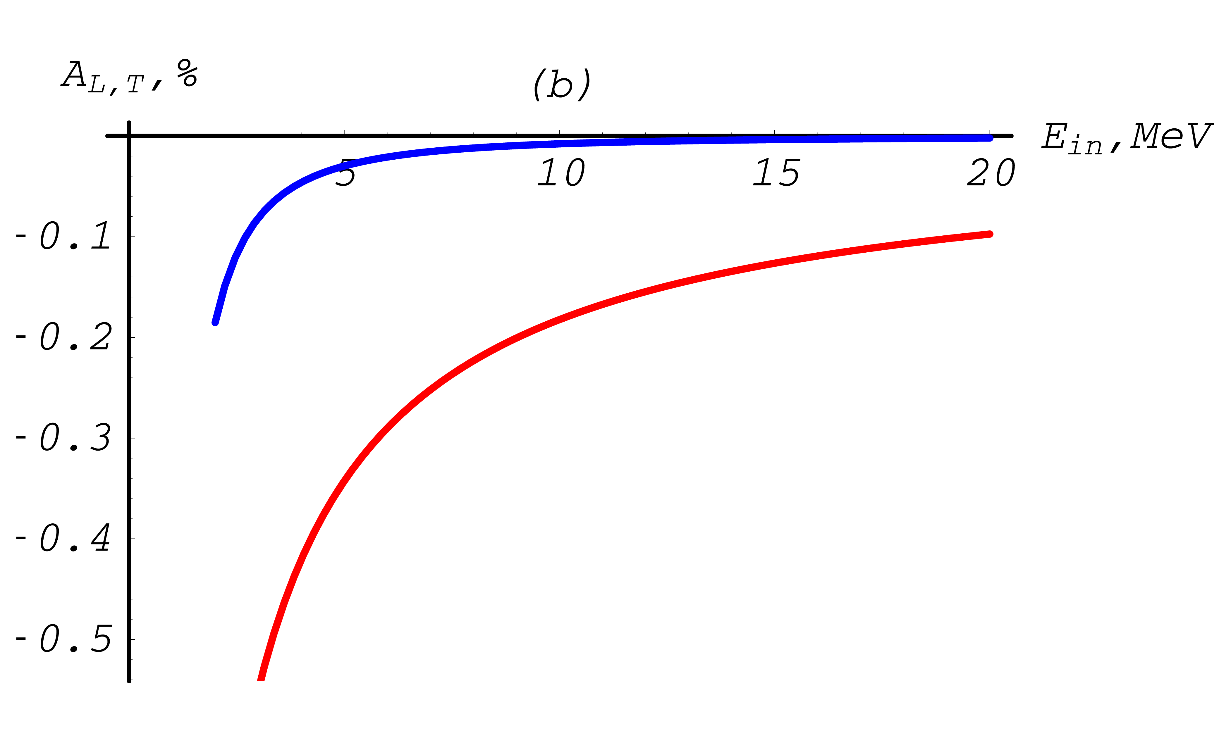
Fig. 34 Møller total cross section asymmetries depending on the total energy of the incoming electron, with a cut-off \(T_{\rm cut}= 1 {\rm keV}\). Transverse asymmetry is plotted in blue, longitudinal asymmetry in red. Up to 10 MeV.

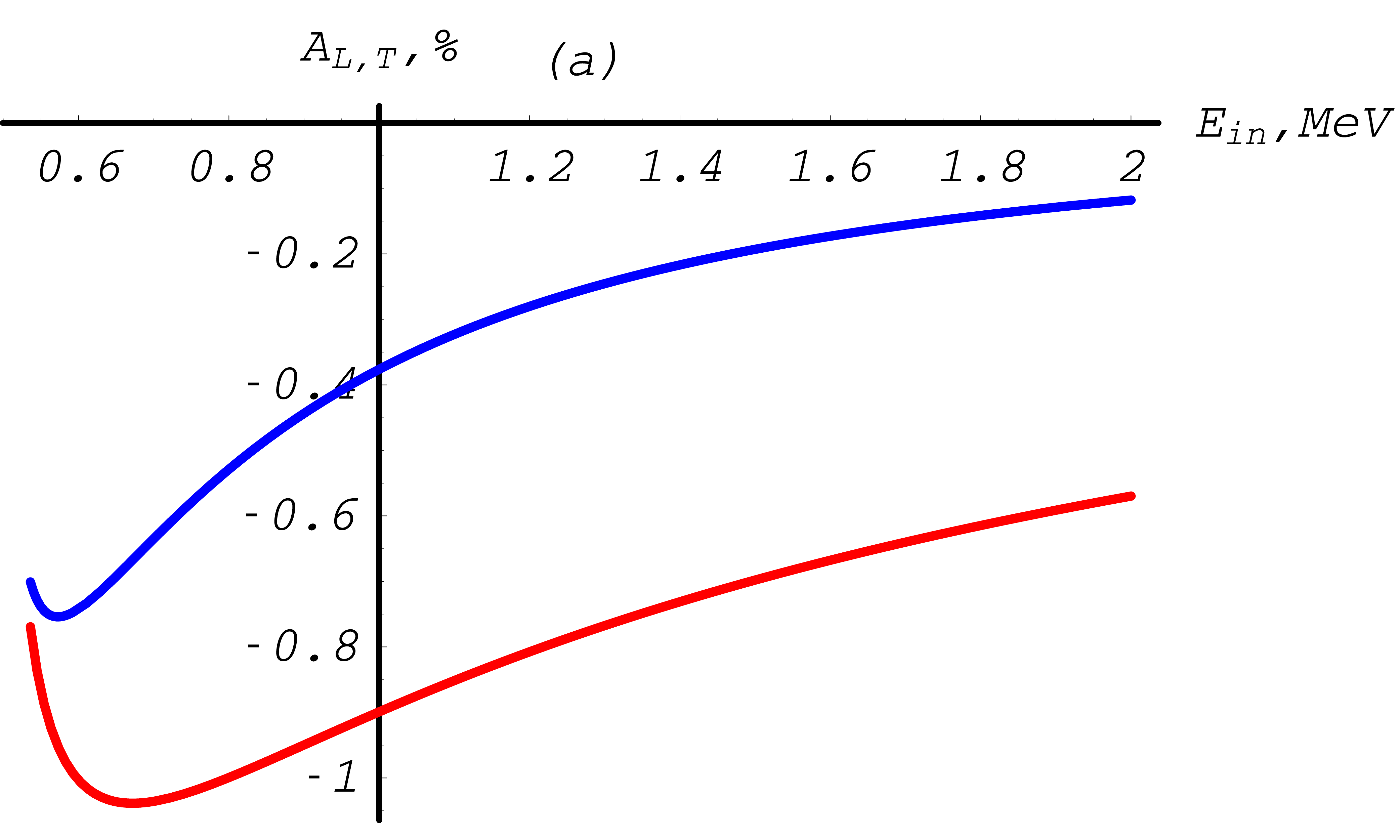
Fig. 35 Bhabha total cross section asymmetries depending on the total energy of the incoming positron, with a cut-off \(T_{\rm cut}= 1 {\rm keV}\). Transverse asymmetry is plotted in blue, longitudinal asymmetry in red. Between 0.5 MeV and 2 MeV.

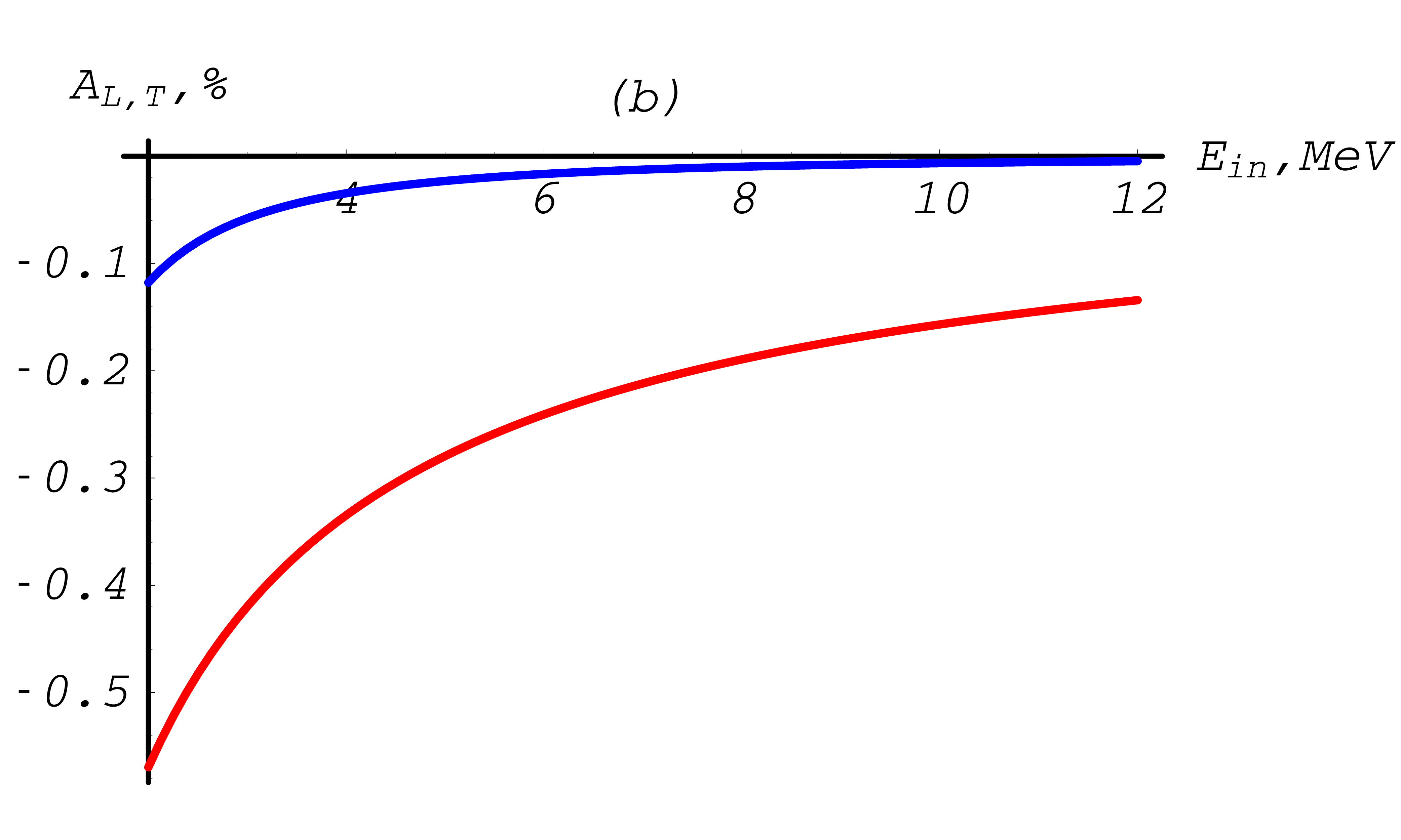
Fig. 36 Bhabha total cross section asymmetries depending on the total energy of the incoming positron, with a cut-off \(T_{\rm cut}= 1 {\rm keV}\). Transverse asymmetry is plotted in blue, longitudinal asymmetry in red. Up to 10 MeV.

Sampling the final state

Differential cross section

The polarized differential cross section is rather complicated. The full result can be found in [eal][FM57][Ste58]. In G4PolarizedMollerCrossSection the complete result is available taking all mass effects into account, with only binding effects neglected. Here we state only the ultra-relativistic approximation (URA), to show the general dependencies.

\[\begin{split}\frac{d\sigma_{URA}^M}{d\epsilon d\varphi} &= \frac{{{r_\epsilon}}^2}{ \gamma + 1} \times \Bigg[ \frac{{\left( 1 - \epsilon + \epsilon^2 \right) }^2}{4\,{\left( \epsilon - 1 \right) }^2\,\epsilon^2} + \zeta_3^{(1)}\zeta_3^{(2)}\frac{2 - \epsilon + \epsilon^2}{-4\,\epsilon ( 1 - \epsilon)} + \left(\zeta_2^{(1)}\zeta_2^{(2)} -\zeta_1^{(1)}\zeta_1^{(2)}\right)\frac{1}{4} \\ &+ \left(\xi_3^{(1)}\zeta_3^{(1)} - \xi_3^{(2)}\zeta_3^{(2)}\right) \frac{1 - \epsilon + 2\,\epsilon^2}{4\,\left( 1 - \epsilon \right) \,\epsilon^2} + \left(\xi_3^{(2)}\zeta_3^{(1)} - \xi_3^{(1)}\zeta_3^{(2)}\right) \frac{2 - 3\,\epsilon + 2\,\epsilon^2}{4\,{\left( 1 - \epsilon \right) }^2\,\epsilon} \Bigg]\end{split}\]

The corresponding cross section for Bhabha cross section is implemented in G4PolarizedBhabhaCrossSection. In the ultra-relativistic approximation it reads

\[\begin{split}\frac{d\sigma_{URA}^B}{d\epsilon d\varphi} &= \frac{{{r_\epsilon}}^2}{ \gamma - 1} \times \Bigg[ \frac{{\left( 1 - \epsilon + \epsilon^2 \right) }^2}{4\,\epsilon^2} + \zeta_3^{(1)}\zeta_3^{(2)}\frac{\left( \epsilon - 1 \right) \,\left( 2 - \epsilon + \epsilon^2 \right) }{4\,\epsilon} +\left(\zeta_2^{(1)}\zeta_2^{(2)} -\zeta_1^{(1)}\zeta_1^{(2)}\right)\frac{(1-\epsilon)^2}{4} \\ &+ \left(\xi_3^{(1)}\zeta_3^{(1)} - \xi_3^{(2)}\zeta_3^{(2)}\right)\frac{1 - 2\,\epsilon + 3\,\epsilon^2 - 2\,\epsilon^3}{4\,\epsilon^2} + \left(\xi_3^{(2)}\zeta_3^{(1)} - \xi_3^{(1)}\zeta_3^{(2)}\right)\frac{ 2 - 3\,\epsilon + 2\,\epsilon^2}{4\epsilon} \Bigg]\end{split}\]

where

\(r_e\)	classical electron radius
\(\gamma\)	\(E_{k_1}/m_e c^2\)
\(\epsilon\)	(\(E_{p_1}-m_e c^2)/(E_{k_1}-m_e c^2)\)
\(E_{k_1}\)	energy of the incident electron/positron
\(E_{p_1}\)	energy of the scattered electron/positron
\(m_e c^2\)	electron mass
\({{\boldsymbol{\zeta}}}^{(1)}\)	Stokes vector of the incoming electron/positron
\({{\boldsymbol{\zeta}}}^{(2)}\)	Stokes vector of the target electron
\({{\boldsymbol{\xi}}}^{(1)}\)	Stokes vector of the outgoing electron/positron
\({{\boldsymbol{\xi}}}^{(2)}\)	Stokes vector of the outgoing (2nd) electron .

Sampling

The delta ray is sampled according to methods discussed in Monte Carlo Methods. After exploitation of the symmetry in the Møller cross section under exchanging \(\epsilon\) versus \((1-\epsilon)\), the differential cross section can be approximated by a simple function \(f^M(\epsilon)\):

\[f^M(\epsilon) = \frac{1}{\epsilon^2} \frac{\epsilon_0}{1-2\epsilon_0}\]

with the kinematic limits given by

\[\epsilon_0 = \frac{T_{\rm cut}}{E_{k_1}-m_e c^2} \le \epsilon \le \frac{1}{2}\]

A similar function \(f^B(\epsilon)\) can be found for Bhabha scattering:

\[f^B(\epsilon) = \frac{1}{\epsilon^2} \frac{\epsilon_0}{1-\epsilon_0}\]

with the kinematic limits given by

\[\epsilon_0 = \frac{T_{\rm cut}}{E_{k_1}-m_e c^2} \le \epsilon \le 1\]

The kinematic of the delta ray production is constructed by the following steps:

1. \(\epsilon\) is sampled from \(f(\epsilon)\)

2. calculate the differential cross section, depending on the initial polarizations \({{\boldsymbol{\zeta}}}^{(1)}\) and \({{\boldsymbol{\zeta}}}^{(2)}\).

3. \(\epsilon\) is accepted with the probability defined by ratio of the differential cross section over the approximation function.

4. The \(\varphi\) is diced uniformly.

5. \(\varphi\) is determined from the differential cross section, depending on the initial polarizations \({{\boldsymbol{\zeta}}}^{(1)}\) and \({{\boldsymbol{\zeta}}}^{(2)}\)

Note, for initial states without transverse polarization components, the \(\varphi\) distribution is always uniform. In Fig. 37 and Fig. 38 the asymmetries indicate the influence of polarization. In general the effect is largest around \(\epsilon=1/2\).

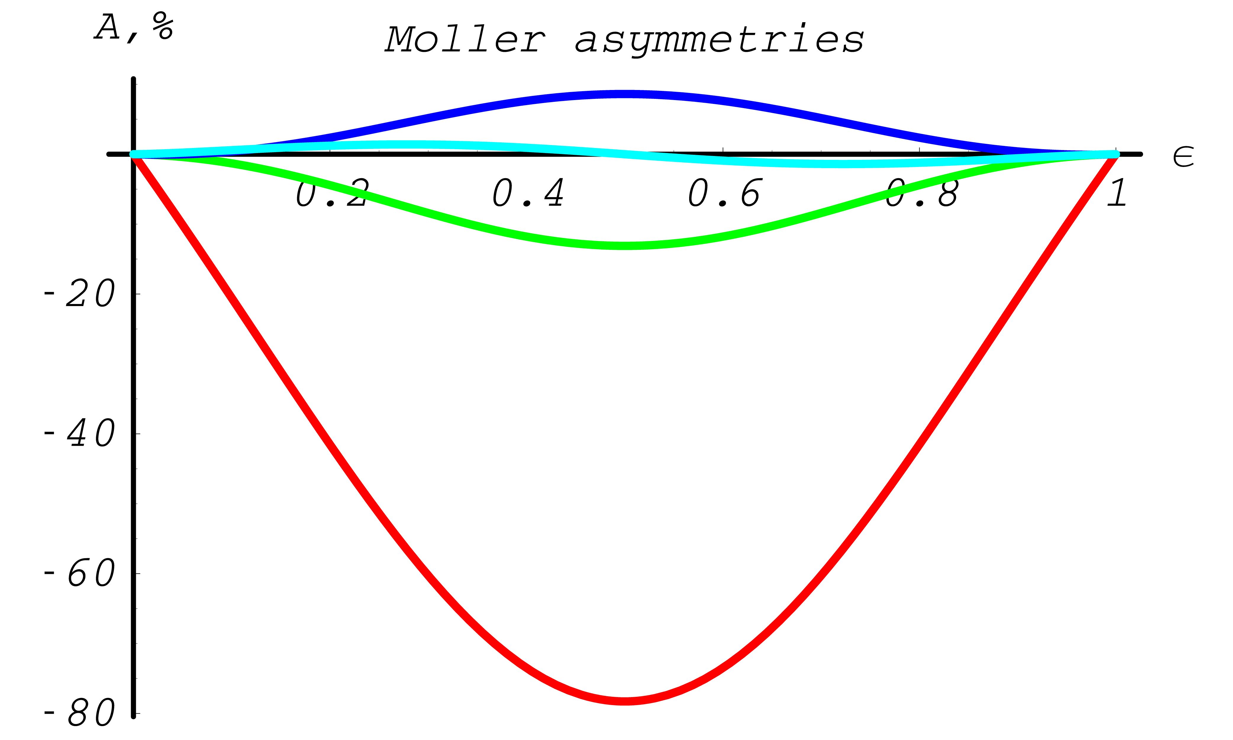
Fig. 37 Differential cross section asymmetries in % for Møller scattering (red - \(A_{ZZ}(\epsilon)\), green - \(A_{XX}(\epsilon)\), blue - \(A_{YY}(\epsilon)\), light blue - \(A_{ZX}(\epsilon)\))

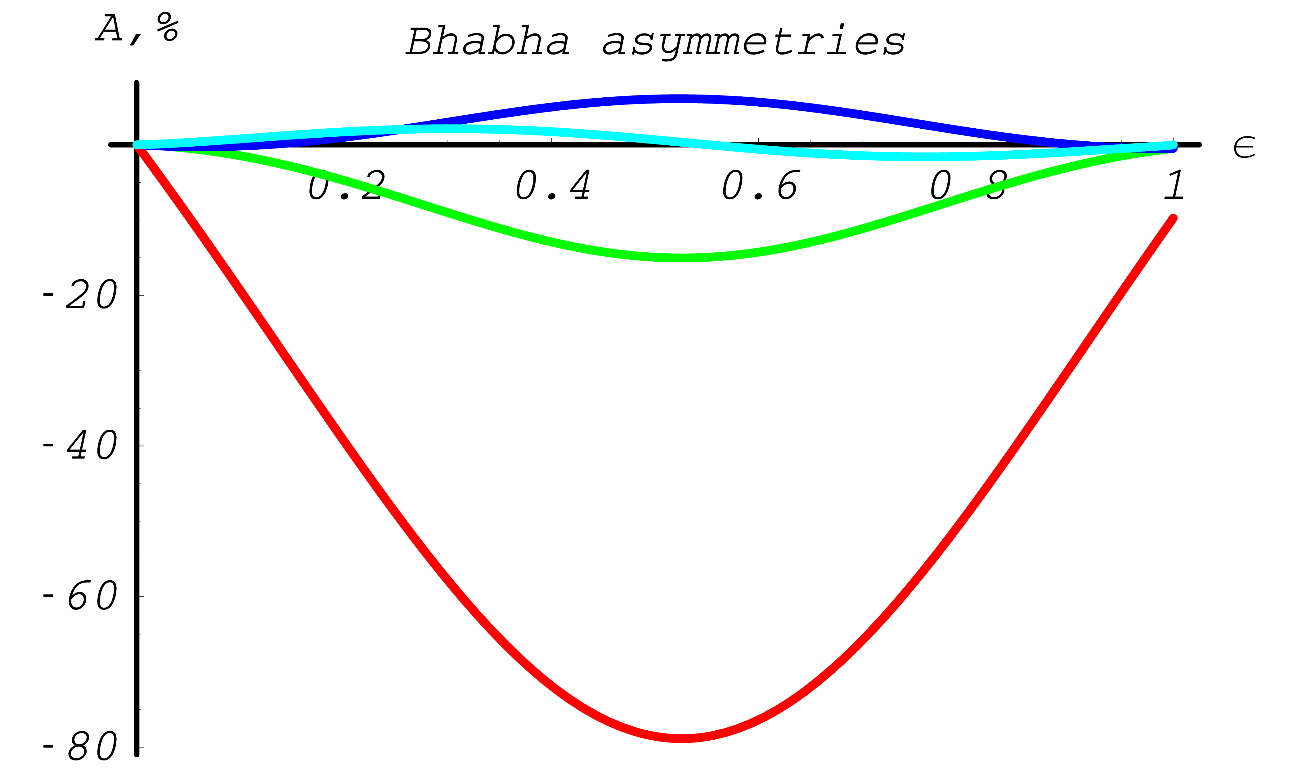
Fig. 38 Differential cross section asymmetries in % for Bhabha scattering (red - \(A_{ZZ}(\epsilon)\), green - \(A_{XX}(\epsilon)\), blue - \(A_{YY}(\epsilon)\), light blue - \(A_{ZX}(\epsilon)\))

After both \(\phi\) and \(\epsilon\) are known, the kinematic can be constructed fully. Using momentum conservation the momenta of the scattered incident particle and the ejected electron are constructed in global coordinate system.

Polarization transfer

After the kinematics is fixed the polarization properties of the outgoing particles are determined. Using the dependence of the differential cross section on the final state polarization a mean polarization is calculated according to method described in Introduction.

The resulting polarization transfer functions \(\xi^{(1,2)}_3(\epsilon)\) are depicted in Fig. 39, Fig. 40, and Fig. 41, Fig. 42.

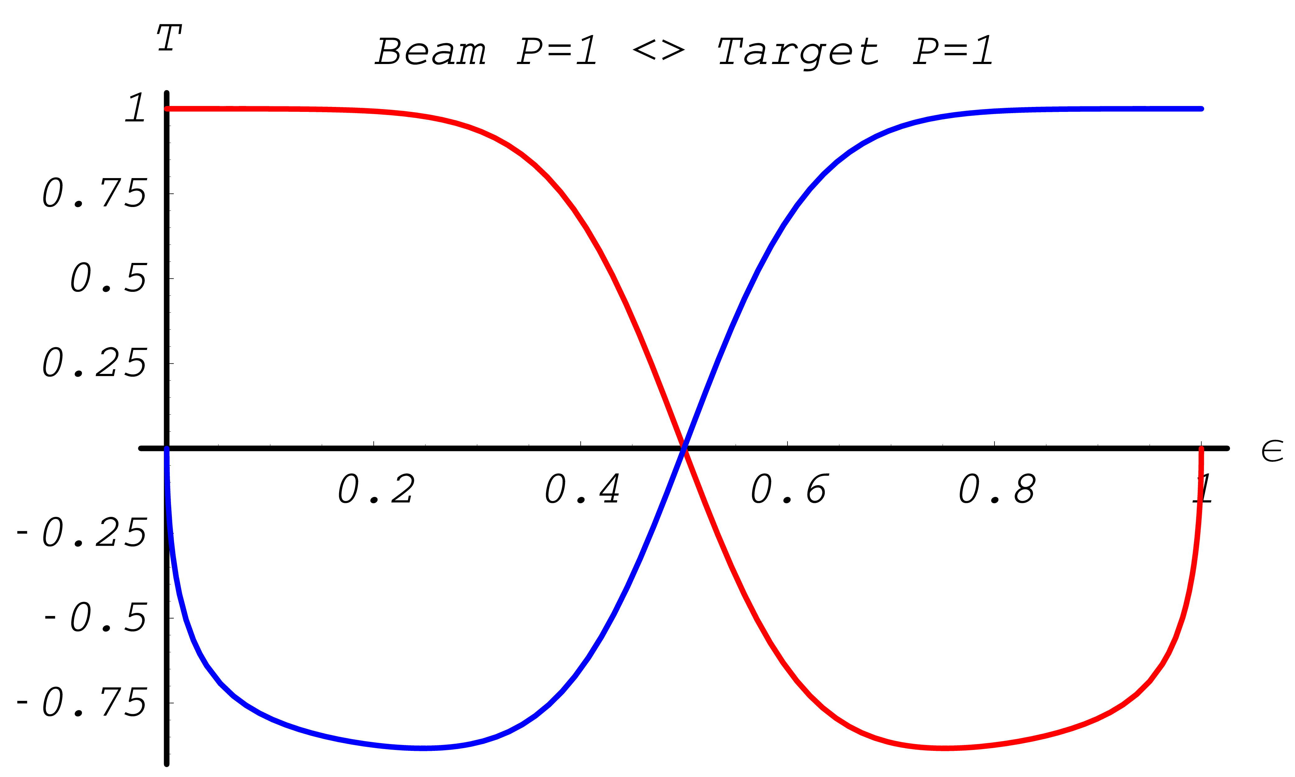
Fig. 39 Polarization transfer functions in Møller scattering. Longitudinal polarization \(\xi^{(2)}_3\) of electron with energy \(E_{p_2}\) in blue; longitudinal polarization \(\xi^{(1)}_3\) of second electron in red. Kinetic energy of incoming electron \(T_{k_1} = 10 {\rm MeV}\)

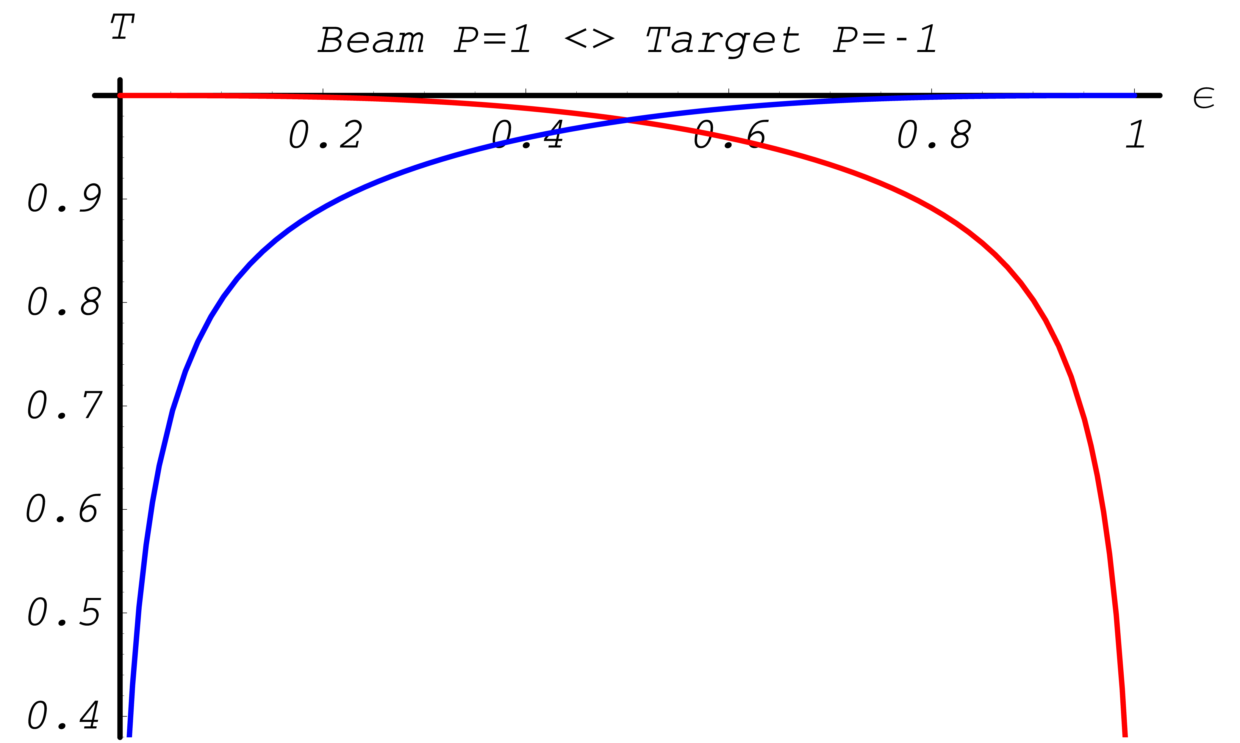
Fig. 40 Polarization transfer functions in Møller scattering. Longitudinal polarization \(\xi^{(2)}_3\) of electron with energy \(E_{p_2}\) in blue; longitudinal polarization \(\xi^{(1)}_3\) of second electron in red. Kinetic energy of incoming electron \(T_{k_1} = 10 {\rm MeV}\)

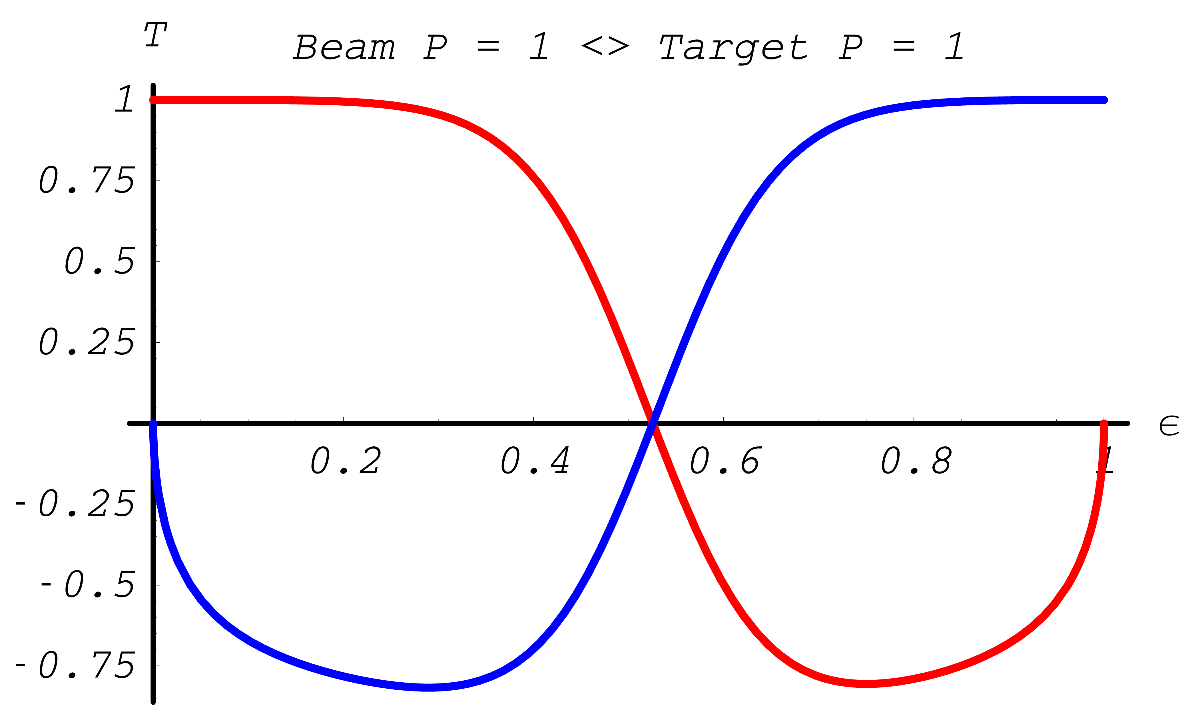
Fig. 41 Polarization Transfer in Bhabha scattering. Longitudinal polarization \(\xi^{(2)}_3\) of electron with energy \(E_{p_2}\) in blue; longitudinal polarization \(\xi^{(1)}_3\) of scattered positron. Kinetic energy of incoming positron \(T_{k_1} = 10 {\rm MeV}\)

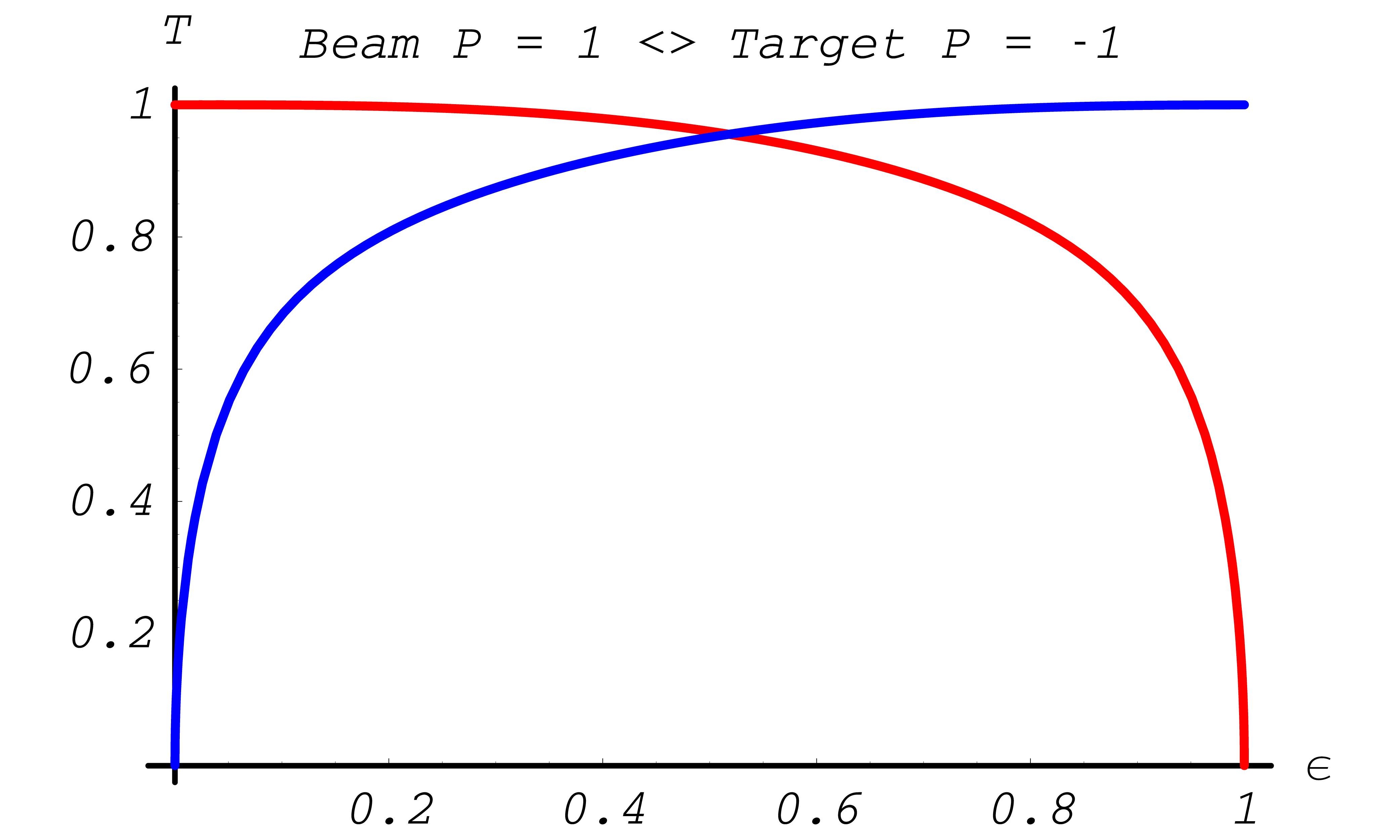
Fig. 42 Polarization Transfer in Bhabha scattering. Longitudinal polarization \(\xi^{(2)}_3\) of electron with energy \(E_{p_2}\) in blue; longitudinal polarization \(\xi^{(1)}_3\) of scattered positron. Kinetic energy of incoming positron \(T_{k_1} = 10 {\rm MeV}\)

Positron - Electron Annihilation

Method

The class G4eplusPolarizedAnnihilation simulates annihilation of polarized positrons with electrons in a material. The implementation baseline follows the approach derived for the class G4eplusAnnihilation described in Positron - Electron Annihilation. It evaluates polarization transfer and – if the material is polarized – asymmetries in the produced photons. Thus, it takes the effects of polarization on total cross section and mean free path, on distribution of final state photons into account. And calculates the average polarization of these generated photons. The material electrons are assumed to be free and at rest.

Total cross section and mean free path

Kinematics of annihilation process is fixed by initial energy

\[\gamma=\frac{E_{k_1}}{mc^2}\]

and variable

\[\epsilon = \frac{E_{p_1}}{E_{k_1}+mc^2},\]

which is the part of total energy available in initial state carried out by first photon. This variable has the following kinematical limits

\[\frac{1}{2}\left(1-\sqrt{\frac{\gamma-1}{\gamma+1}}\right)\;<\; \epsilon \;<\;\frac{1}{2}\left(1+\sqrt{\frac{\gamma-1}{\gamma+1}}\right) \;.\]

Total Cross Section

The total cross section of the annihilation of a polarized \(e^+e^-\) pair into two photons could be expressed as follows

\[\sigma^A_{pol}=\frac{\pi r_e^2}{\gamma+1}\left[ \sigma^A_0 + \zeta_3^{(1)}\zeta_3^{(2)}\sigma^A_L + \left(\zeta_1^{(1)}\zeta_1^{(2)}+\zeta_2^{(1)}\zeta_2^{(2)}\right)\sigma^A_T\right],\]

where

\[\begin{split}\sigma^A_0 &= \frac{- \left( 3 + {\gamma} \right) \,{\sqrt{-1 + {{\gamma}}^2}} + \left( 1 + {\gamma}\,\left( 4 + {\gamma} \right) \right) \, \ln ({\gamma} + {\sqrt{-1 + {{\gamma}}^2}})}{4\, \left( {{\gamma}}^2 - 1 \right) } \\ \sigma^A_L &= \frac{- {\sqrt{-1 + {{\gamma}}^2}}\, \left( 5 + {\gamma}\,\left( 4 + 3\,{\gamma} \right) \right) + \left( 3 + {\gamma}\,\left( 7 + {\gamma} + {{\gamma}}^2 \right) \right) \, \ln ({\gamma} + {\sqrt{{{\gamma}}^2-1 }})}{4\, {\left( {\gamma} -1\right) }^2\,\left( 1 + {\gamma} \right) } \\ \sigma^A_T &= \frac{\left( 5 + {\gamma} \right) \,{\sqrt{-1 + {{\gamma}}^2}} - \left( 1 + 5\,{\gamma} \right) \,\ln ({\gamma} + {\sqrt{-1 + {{\gamma}}^2}})} {4\,{\left( -1 + {\gamma} \right) }^2\,\left( 1 + {\gamma} \right) }\end{split}\]

Mean free path

With the help of the total polarized annihilation cross section one can define a longitudinal asymmetry \(A^A_L\) and the transverse asymmetry \(A^A_T\), by

\[A^A_L = \displaystyle \frac{\sigma^A_L}{\sigma^A_0}\]

and

\[A^A_T = \displaystyle \frac{\sigma^A_T}{\sigma^A_0}.\]

These asymmetries are depicted in Fig. 43, Fig. 44.

If both incident positron and target electron are polarized the mean free path as defined in section Positron - Electron Annihilation has to be modified. The polarized mean free path \(\lambda^{\rm pol}\) is derived from the unpolarized mean free path \(\lambda^{\rm unpol}\) via

\[\lambda^{\rm pol} = \frac{\lambda^{\rm unpol}}{1 + \zeta_3^{(1)}\zeta_3^{(2)}\, A_L + \left(\zeta_1^{(1)}\zeta_1^{(2)}+\zeta_2^{(1)}\zeta_2^{(2)}\right) \,A_T}\]

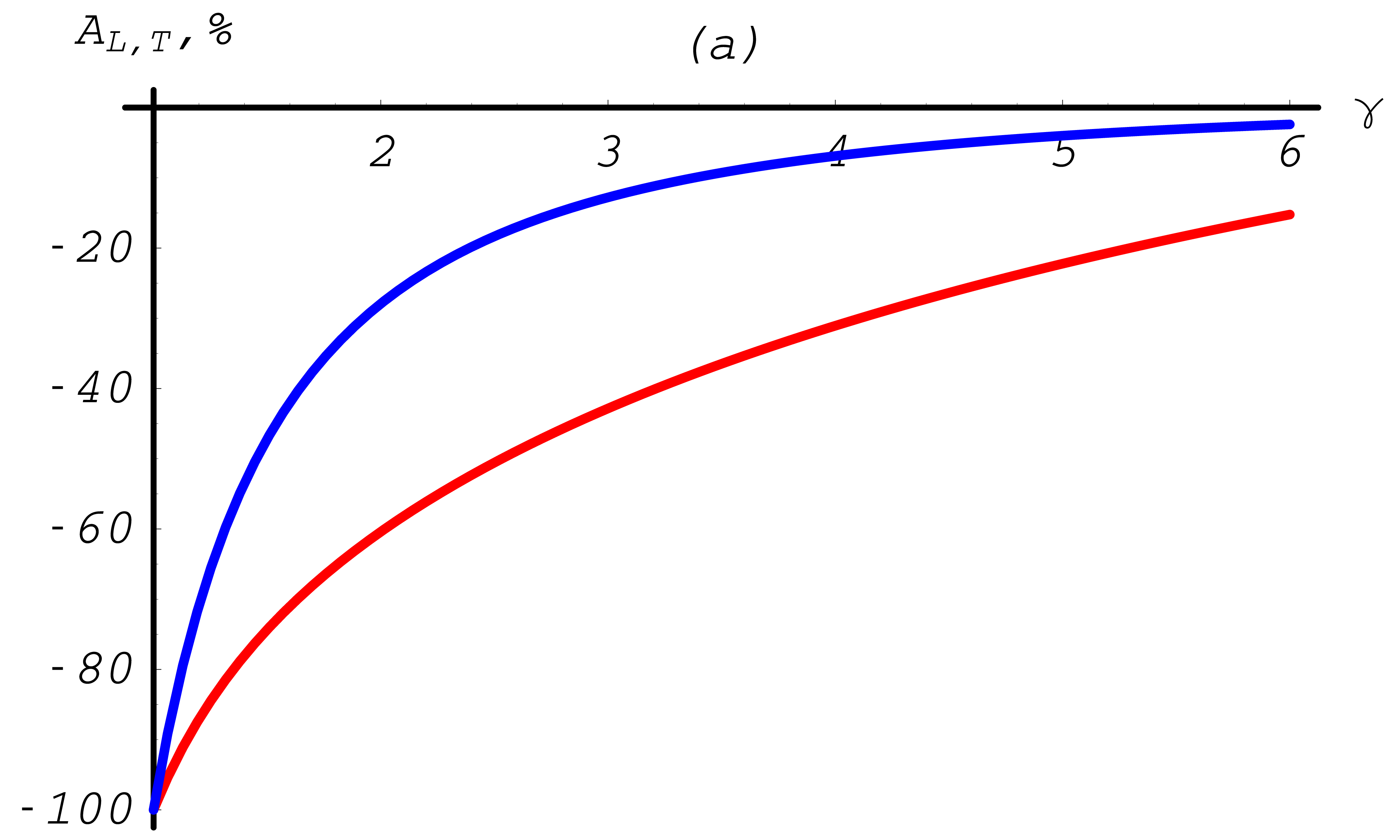
Fig. 43 Annihilation total cross section asymmetries depending on the total energy of the incoming positron \(E_{k_1}\). The transverse asymmetry is shown in blue, the longitudinal asymmetry in red.

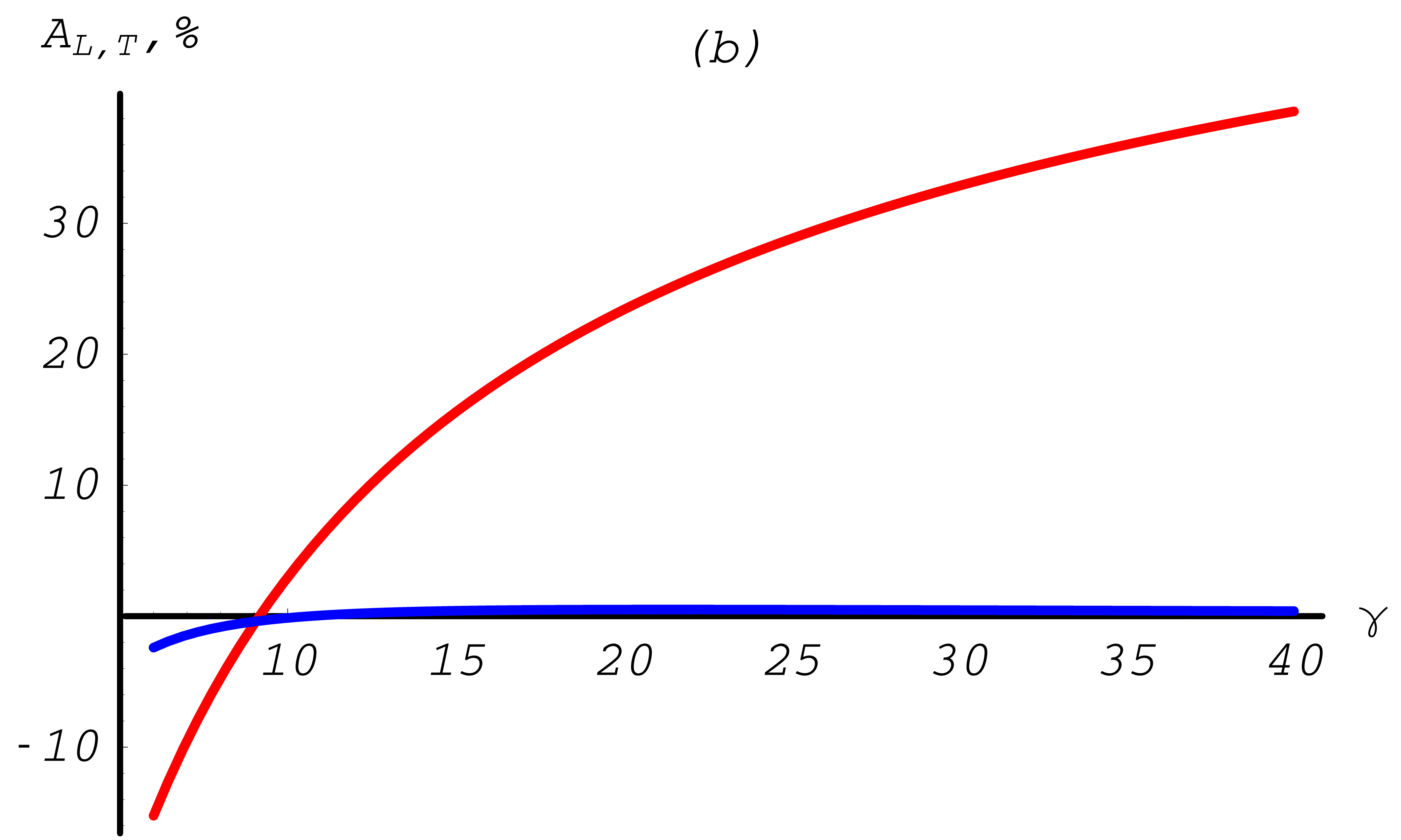
Fig. 44 Annihilation total cross section asymmetries depending on the total energy of the incoming positron \(E_{k_1}\). The transverse asymmetry is shown in blue, the longitudinal asymmetry in red.

Sampling the final state

Differential Cross Section

The fully polarized differential cross section is implemented in the class G4PolarizedAnnihilationCrossSection, which takes all mass effects into account, but binding effects are neglected [eal][Pag57]. In the ultra-relativistic approximation (URA) and concentrating on longitudinal polarization states only the cross section is rather simple:

\[\frac{d\sigma_{URA}^A}{d\epsilon d\varphi} = \frac{{{r_e}}^2}{ \gamma - 1} \times \Bigg( \frac{1 - 2\,\epsilon + 2\,\epsilon^2}{8\,\epsilon - 8\,\epsilon^2}\left(1 + \zeta_3^{(1)}\zeta_3^{(2)}\right) + \frac{ \left( 1 - 2\,\epsilon \right) \,\left( \zeta _{3}^{(1)} + \zeta _{3}^{(2)} \right) \, \left( \xi _{3}^{(1)} - \xi _{3}^{(2)} \right) }{8\,\left( \epsilon -1 \right) \,\epsilon} \Bigg)\]

where

\(r_e\)	classical electron radius
\(\gamma\)	\(E_{k_1}/m_e c^2\)
\(E_{k_1}\)	energy of the incident positron
\(m_e c^2\)	electron mass
\({{\boldsymbol{\zeta}}}^{(1)}\)	Stokes vector of the incoming positron
\({{\boldsymbol{\zeta}}}^{(2)}\)	Stokes vector of the target electron
\({{\boldsymbol{\xi}}}^{(1)}\)	Stokes vector of the 1st photon
\({{\boldsymbol{\xi}}}^{(2)}\)	Stokes vector of the 2nd photon .

Sampling

The photon energy is sampled according to methods discussed in Monte Carlo Methods. After exploitation of the symmetry in the Annihilation cross section under exchanging \(\epsilon\) versus \((1-\epsilon)\), the differential cross section can be approximated by a simple function \(f(\epsilon)\):

\[f(\epsilon) = \frac{1}{\epsilon} \ln^{-1}\left(\frac{\epsilon_{\rm max}}{\epsilon_{\rm min}}\right)\]

with the kinematic limits given by

\[\begin{split}\epsilon_{\rm min} &= \frac{1}{2}\left(1-\sqrt{\frac{\gamma-1}{\gamma+1}}\right)\;, \\ \epsilon_{\rm max} &= \frac{1}{2}\left(1+\sqrt{\frac{\gamma-1}{\gamma+1}}\right) \;.\end{split}\]

The kinematic of the two photon final state is constructed by the following steps:

1. \(\epsilon\) is sampled from \(f(\epsilon)\)

2. calculate the differential cross section, depending on the initial polarizations \({{\boldsymbol{\zeta}}}^{(1)}\) and \({{\boldsymbol{\zeta}}}^{(2)}\).

3. \(\epsilon\) is accepted with the probability defined by the ratio of the differential cross section over the approximation function \(f(\epsilon)\).

4. The \(\varphi\) is diced uniformly.

5. \(\varphi\) is determined from the differential cross section, depending on the initial polarizations \({{\boldsymbol{\zeta}}}^{(1)}\) and \({{\boldsymbol{\zeta}}}^{(2)}\).

A short overview over the sampling method is given in Monte Carlo Methods. In Fig. 45 the asymmetries indicate the influence of polarization for an 10MeV incoming positron. The actual behavior is very sensitive to the energy of the incoming positron.

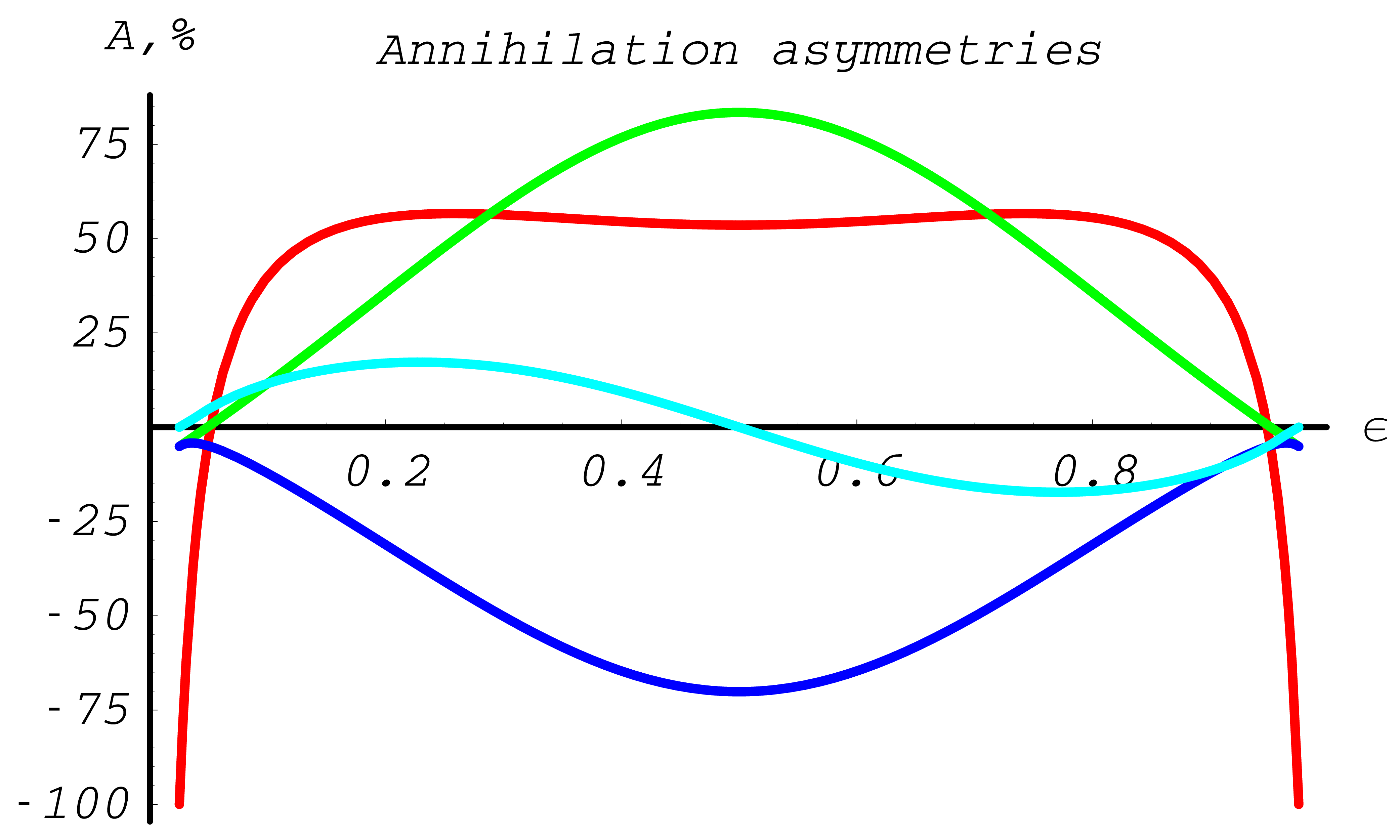
Fig. 45 Annihilation differential cross section asymmetries in %. Red line corrsponds to \(A_{ZZ}(\epsilon)\), green line – \(A_{XX}(\epsilon)\), blue line – \(A_{YY}(\epsilon)\), lightblue line – \(A_{ZX}(\epsilon)\)). Kinetic energy of the incoming positron \(T_{k_1} = 10 {\rm MeV}\).

Polarization transfer

After the kinematics is fixed the polarization of the outgoing photon is determined. Using the dependence of the differential cross section on the final state polarizations a mean polarization is calculated for each photon according to method described in section Introduction.

The resulting polarization transfer functions \(\xi^{(1,2)}(\epsilon)\) are depicted in Fig. 46, Fig. 47.

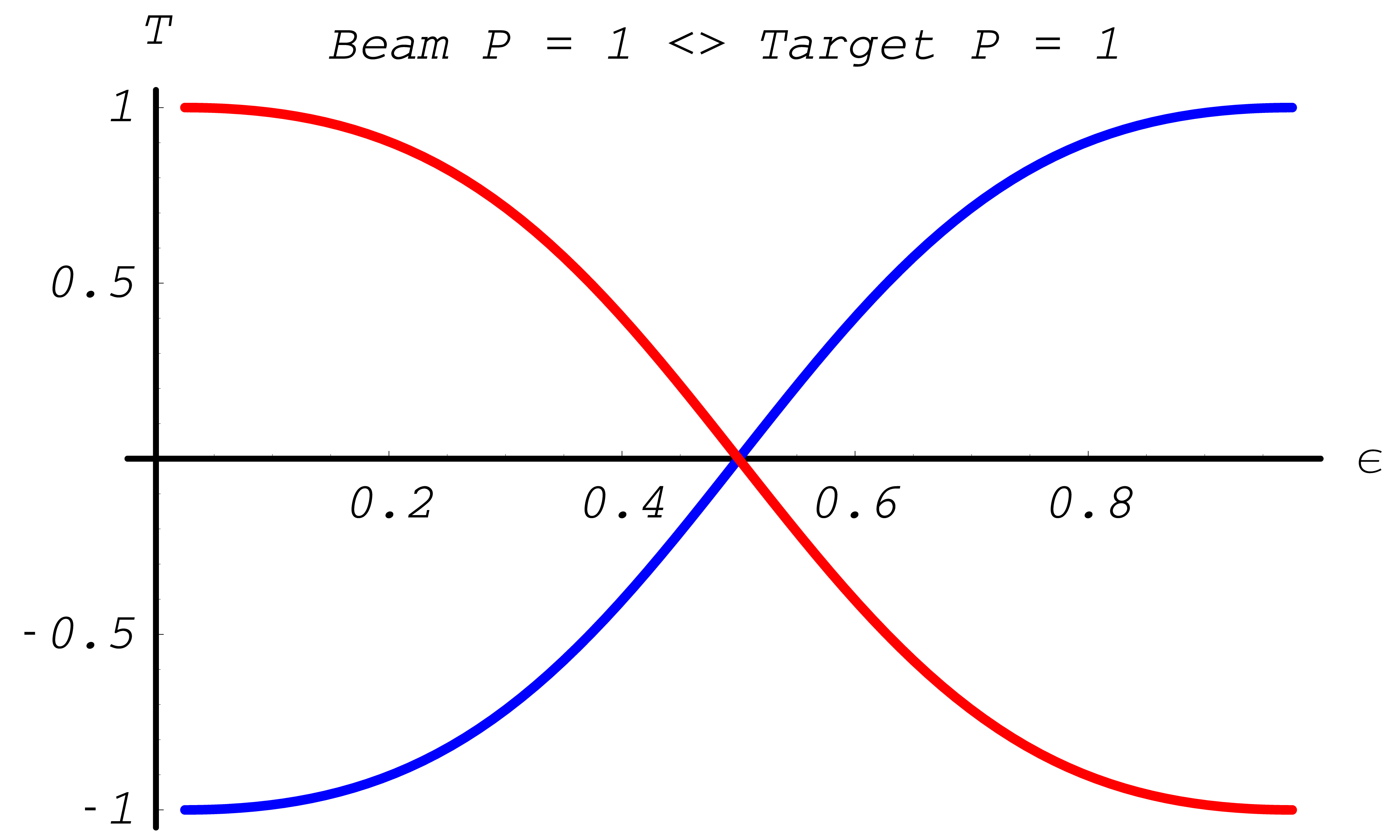
Fig. 46 Polarization Transfer in annihilation process. Blue line corresponds to the circular polarization \(\xi_3^{(1)}\) of the photon with energy \(m(\gamma + 1)\epsilon\); red line – circular polarization \(\xi_3^{(2)}\) of the photon photon with energy \(m(\gamma + 1)(1-\epsilon)\).

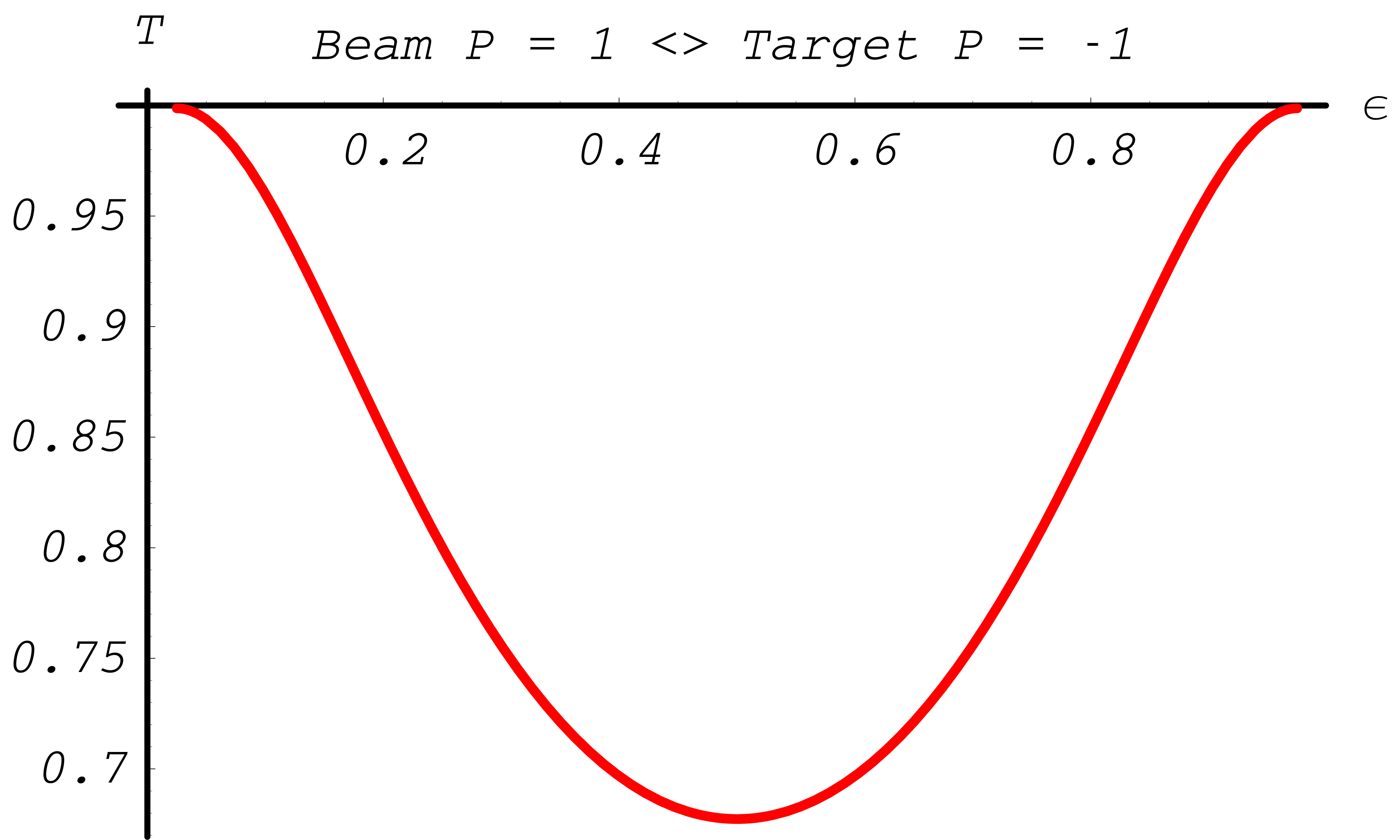
Fig. 47 Polarization Transfer in annihilation process. Blue line corresponds to the circular polarization \(\xi_3^{(1)}\) of the photon with energy \(m(\gamma + 1)\epsilon\); red line – circular polarization \(\xi_3^{(2)}\) of the photon photon with energy \(m(\gamma + 1)(1-\epsilon)\).

Annihilation at Rest

The method AtRestDoIt treats the special case where a positron comes to rest before annihilating. It generates two photons, each with energy \(E_{p_{1/2}}=m c^2\) and an isotropic angular distribution. Starting with the differential cross section for annihilation with positron and electron spins opposed and parallel, respectively, [Pag57]

\[\begin{split}d\sigma_1 &= \sim \frac{(1 - \beta^2) + \beta^2 (1 - \beta^2) (1 - \cos^2\theta)^2}{(1 - \beta^2\cos^2\theta)^2} d \cos\theta \\ d\sigma_2 &= \sim \frac{\beta^2(1 - \cos^4\theta)}{(1 - \beta^2\cos^2\theta)^2} d \cos\theta\end{split}\]

In the limit \(\beta\to0\) the cross section \(d\sigma_1\) becomes one, and the cross section \(d\sigma_2\) vanishes. For the opposed spin state, the total angular momentum is zero and we have a uniform photon distribution. For the parallel case the total angular momentum is 1. Here the two photon final state is forbidden by angular momentum conservation, and it can be assumed that higher order processes (e.g. three photon final state) play a dominant role. However, in reality 100% polarized electron targets do not exist, consequently there are always electrons with opposite spin, where the positron can annihilate with. Final state polarization does not play a role for the decay products of a spin zero state, and can be safely neglected (is set to zero).

Polarized Compton scattering

Method

The class G4PolarizedCompton simulates Compton scattering of polarized photons with (possibly polarized) electrons in a material. The implementation follows the approach described for the class G4ComptonScattering introduced in Compton scattering. Here the explicit production of a Compton scattered photon and the ejected electron is considered taking the effects of polarization on total cross section and mean free path as well as on the distribution of final state particles into account. Further the average polarizations of the scattered photon and electron are calculated. The material electrons are assumed to be free and at rest.

Total cross section and mean free path

Kinematics of the Compton process is fixed by the initial energy

\[X=\frac{E_{k_1}}{mc^2}\]

and the variable

\[\epsilon = \frac{E_{p_1}}{E_{k_1}},\]

which is the part of total energy available in initial state carried out by scattered photon, and the scattering angle

\[\cos{\theta} = 1 - \frac{1}{X}\left(\frac{1}{\epsilon} - 1\right)\]

The variable \(\epsilon\) has the following limits:

\[\frac{1}{1+2X} \;<\; \epsilon \;<\;1\]

Total Cross Section

The total cross section of Compton scattering reads

\[\sigma^{C}_{pol}= \frac{\pi \,{{r_e}}^2}{X^2\,{\left( 1 + 2\,X \right) }^2} \left[\sigma^{C}_0 + \zeta^{(1)}_3\zeta^{(2)}_3 \sigma^{C}_L\right]\]

where

\[\sigma^{C}_0 = \frac{2\,X\,\left( 2 + X\,\left( 1 + X \right) \,\left( 8 + X \right) \right) - {\left( 1 + 2\,X \right) }^2\,\left( 2 + \left( 2 - X \right) \,X \right) \, \ln (1 + 2\,X)}{X}\]

and

\[\sigma^{C}_L = 2\,X\,\left( 1 + X\,\left( 4 + 5\,X \right) \right) - \left( 1 + X \right) \,{\left( 1 + 2\,X \right) }^2\,\ln (1 + 2\,X)\]

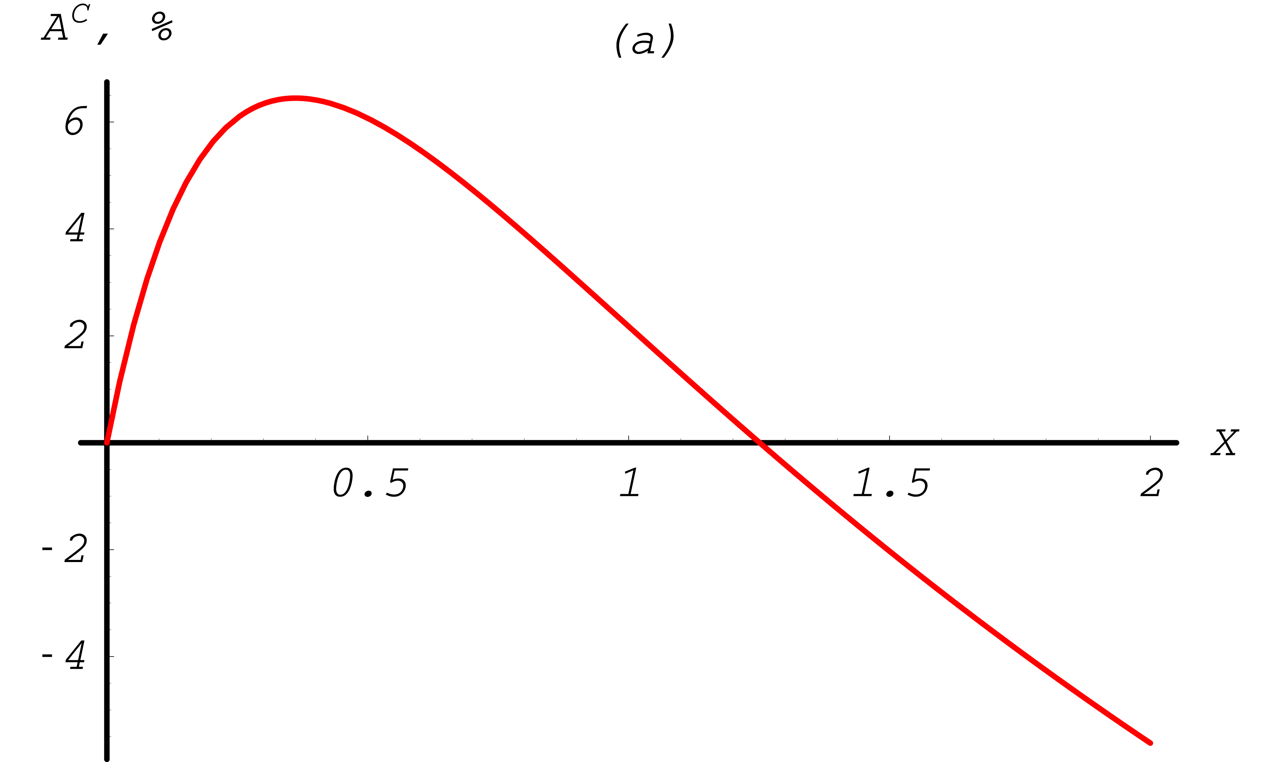
Fig. 48 Compton total cross section asymmetry depending on the energy of incoming photon. Between \(0\) and \(\sim 1\) MeV.

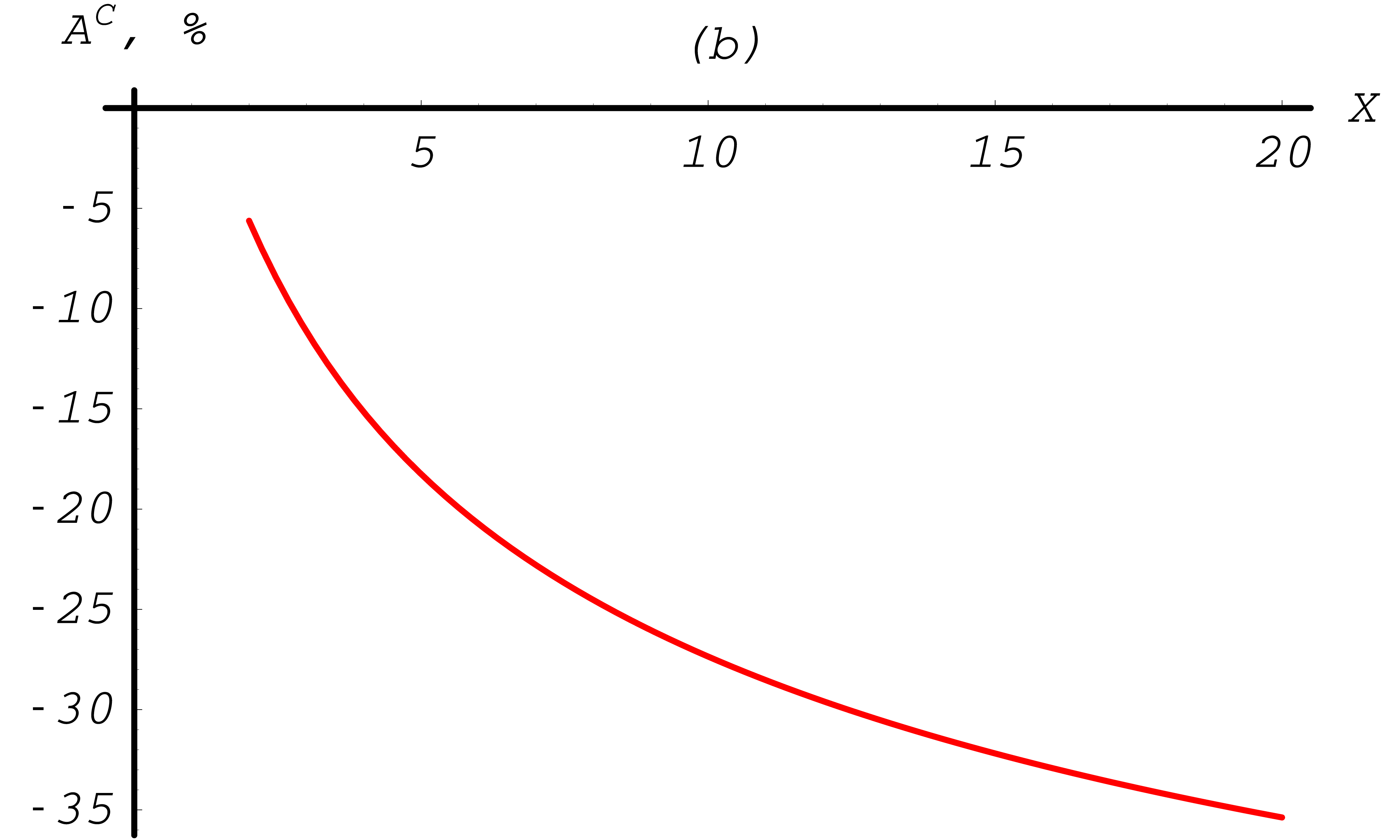
Fig. 49 Compton total cross section asymmetry depending on the energy of incoming photon. Up to 10MeV.

Mean free path

When simulating the Compton scattering of a photon with an atomic electron, an empirical cross section formula is used, which reproduces the cross section data down to 10 keV (see Compton scattering). If both beam and target are polarized this mean free path has to be corrected.

In the class G4ComptonScattering the polarized mean free path \(\lambda^{\rm pol}\) is defined on the basis of the the unpolarized mean free path \(\lambda^{\rm unpol}\) via

\[\lambda^{\rm pol} = \frac{\lambda^{\rm unpol}}{1 + \zeta_3^{(1)}\zeta_3^{(2)}\, A^C_L }\]

where

\[A^C_L = \displaystyle \frac{\sigma^A_L}{\sigma^A_0}\]

is the expected asymmetry from the the total polarized Compton cross section given above. This asymmetry is depicted in Fig. 48, Fig. 49.

Sampling the final state

Differential Compton Cross Section

In the ultra-relativistic approximation the dependence of the differential cross section on the longitudinal/circular degree of polarization is very simple. It reads

\[\frac{d\sigma_{URA}^C}{de d\varphi}= \frac{{{r_e}}^2 }{ X} \Bigg( \frac{\epsilon^2 + 1}{2\,\epsilon} + \frac{ \epsilon^2 -1 }{2\,\epsilon} \left(\zeta_3^{(1)}\zeta_3^{(2)} + \zeta _{3}^{(2)}\,\xi _{3}^{(1)} - \zeta _{3}^{(1)}\,\xi _{3}^{(2)}\right) +\frac{\epsilon^2 + 1}{2\,\epsilon} \left( \zeta _{3}^{(1)}\,\xi _{3}^{(1)} - \zeta _{3}^{(2)} \,\xi _{3}^{(2)} \right) \Bigg)\]

where

\(r_e\)	classical electron radius
\(X\)	\(E_{k_1}/m_e c^2\)
\(E_{k_1}\)	energy of the incident photon
\(m_e c^2\)	electron mass

The fully polarized differential cross section is available in the class G4PolarizedComptonCrossSection. It takes all mass effects into account, but binding effects are neglected [eal][LT54a][LT54b]. The cross section dependence on \(\epsilon\) for right handed circularly polarized photons and longitudinally polarized electrons is plotted in Fig. 50, Fig. 51.

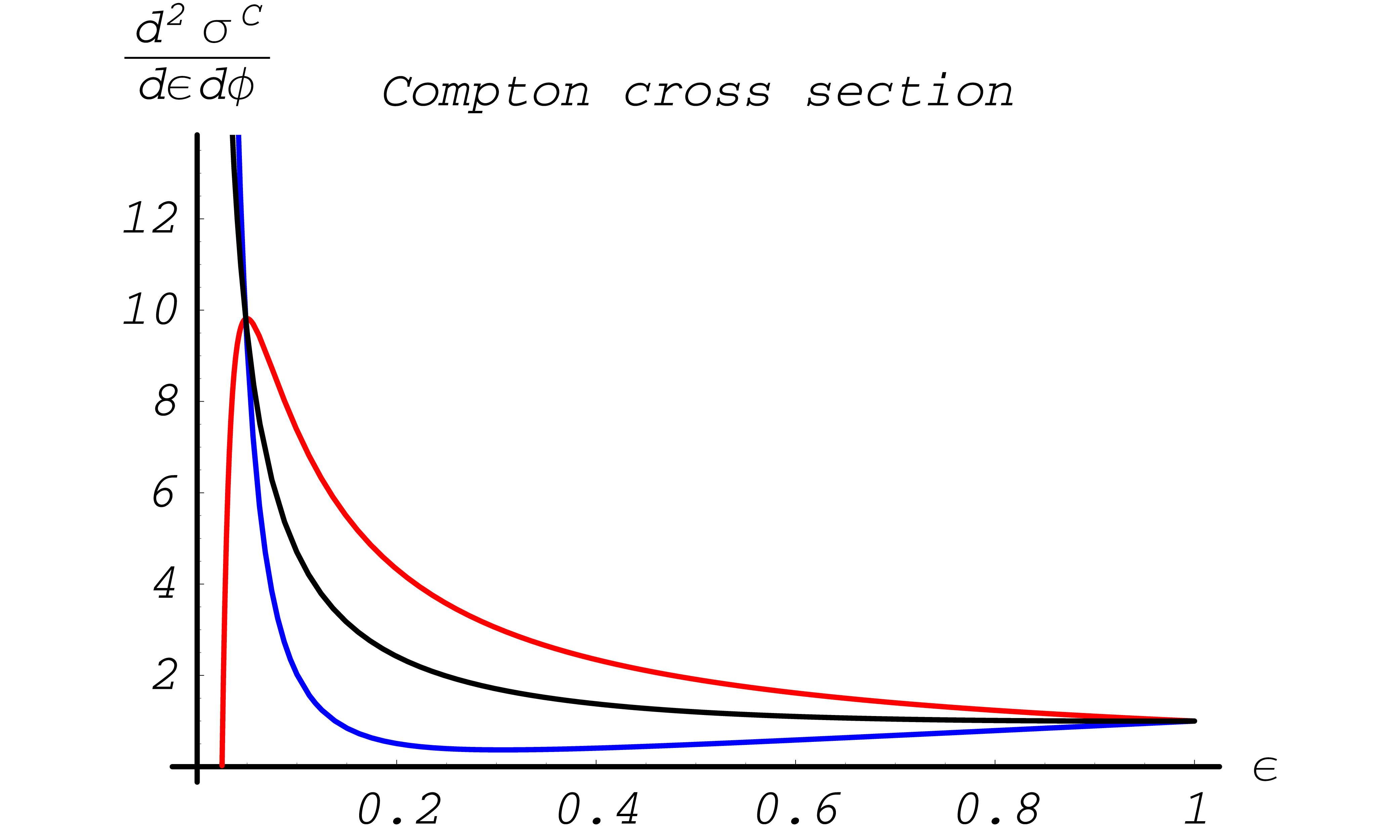
Fig. 50 Compton scattering differential cross section in arbitrary units. Black line corresponds to the unpolarized cross section; red line – to the antiparallel spins of initial particles, and blue line – to the parallel spins. Energy of the incoming photon \(E_{k_1} = 10 {\rm MeV}\).

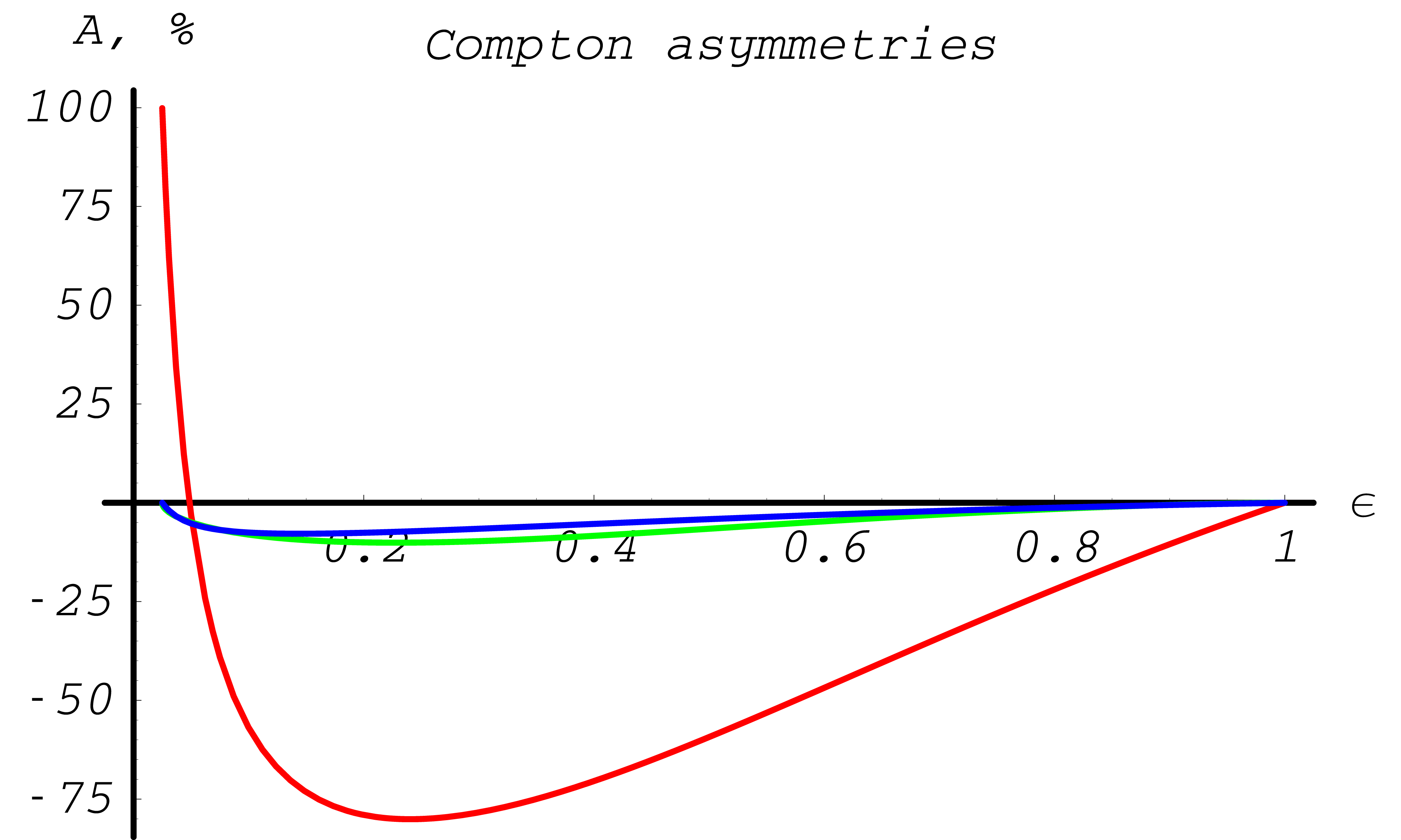
Fig. 51 Compton scattering differential cross section asymmetries in%. Red line corresponds to the asymmetry due to circular photon and longitudinal electron initial state polarization, green line – due to circular photon and transverse electron initial state polarization, blue line – due to linear photon and transverse electron initial state polarization.

Sampling

The photon energy is sampled according to methods discussed in Monte Carlo Methods. The differential cross section can be approximated by a simple function \(\Phi(\epsilon)\):

\[\Phi(\epsilon) = \frac{1}{\epsilon} + \epsilon\]

with the kinematic limits given by

\[\begin{split}\epsilon_{\rm min} &= \frac{1}{1+2X} \\ \epsilon_{\rm max} &= 1\end{split}\]

The kinematic of the scattered photon is constructed by the following steps:

1. \(\epsilon\) is sampled from \(\Phi(\epsilon)\)

2. calculate the differential cross section, depending on the initial polarizations \({{\boldsymbol{\zeta}}}^{(1)}\) and \({{\boldsymbol{\zeta}}}^{(2)}\), which the correct normalization.

3. \(\epsilon\) is accepted with the probability defined by ratio of the differential cross section over the approximation function.

4. The \(\varphi\) is diced uniformly.

5. \(\varphi\) is determined from the differential cross section, depending on the initial polarizations \({{\boldsymbol{\zeta}}}^{(1)}\) and \({{\boldsymbol{\zeta}}}^{(2)}\).

In Fig. 50, Fig. 51 the asymmetries indicate the influence of polarization for an 10 MeV incoming positron. The actual behavior is very sensitive to energy of the incoming positron.

Polarization transfer

After the kinematics is fixed the polarization of the outgoing photon is determined. Using the dependence of the differential cross section on the final state polarizations a mean polarization is calculated for each photon according to the method described in section Introduction.

The resulting polarization transfer functions \(\xi^{(1,2)}(\epsilon)\) are depicted in Fig. 52, Fig. 53.

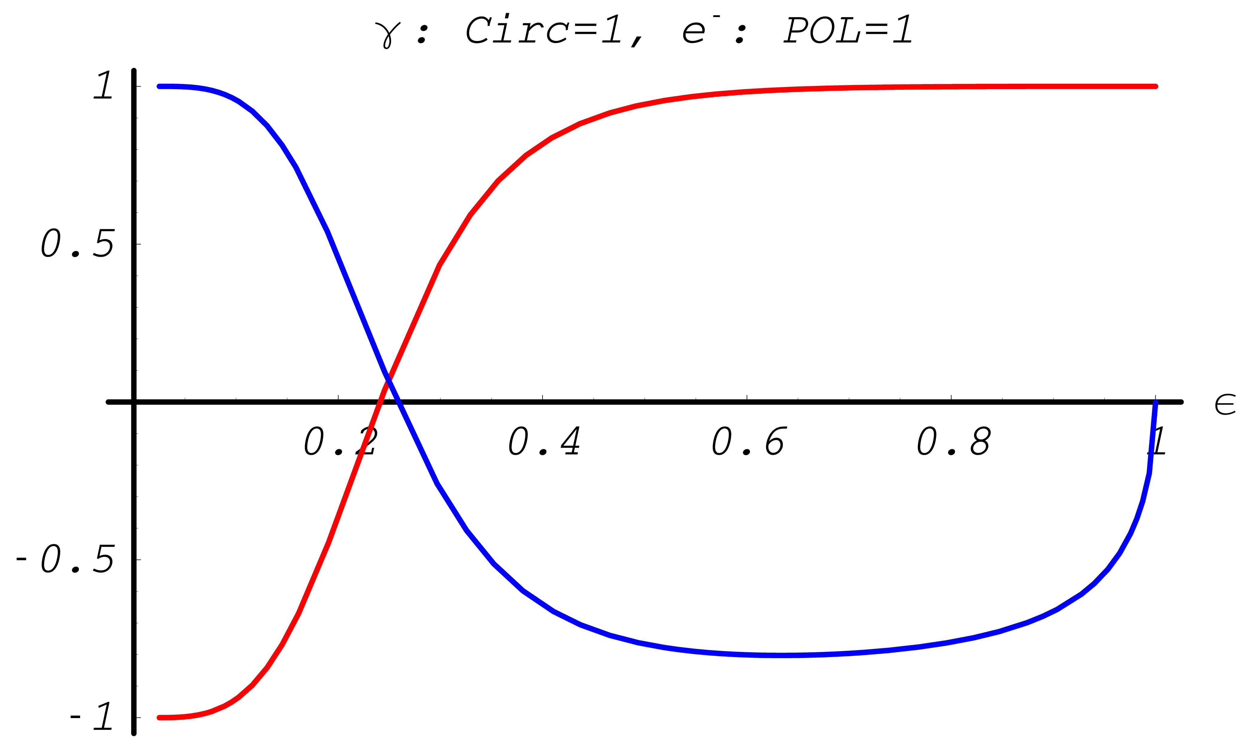
Fig. 52 Polarization Transfer in Compton scattering. Blue line corresponds to the longitudinal polarization \(\xi_3^{(2)}\) of the electron, red line – circular polarization \(\xi_3^{(1)}\) of the photon.

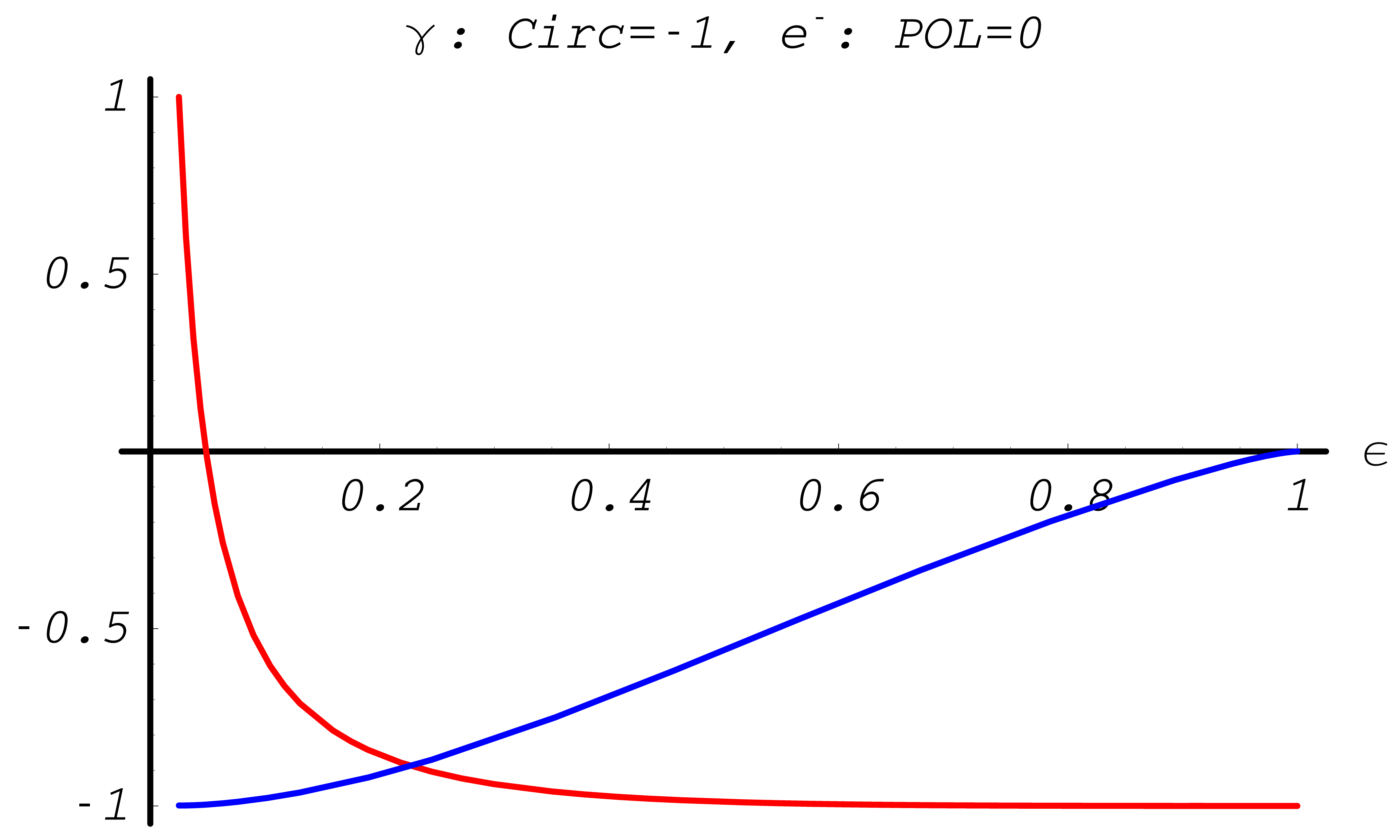
Fig. 53 Polarization Transfer in Compton scattering. Blue line corresponds to the longitudinal polarization \(\xi_3^{(2)}\) of the electron, red line – circular polarization \(\xi_3^{(1)}\) of the photon.

Polarized Bremsstrahlung for electron and positron

Method

The polarized version of Bremsstrahlung is based on the unpolarized cross section. Energy loss, mean free path, and distribution of explicitly generated final state particles are treated by the unpolarized version G4eBremsstrahlung. For details consult Bremsstrahlung.

The remaining task is to attribute polarization vectors to the generated final state particles, which is discussed in the following.

Polarization in gamma conversion and bremsstrahlung

Gamma conversion and bremsstrahlung are cross-symmetric processes (i.e. the Feynman diagram for electron bremsstrahlung can be obtained from the gamma conversion diagram by flipping the incoming photon and outgoing positron lines) and their cross sections closely related. For both processes, the interaction occurs in the field of the nucleus and the total and differential cross section are polarization independent. Therefore, only the polarization transfer from the polarized incoming particle to the outgoing particles is taken into account.

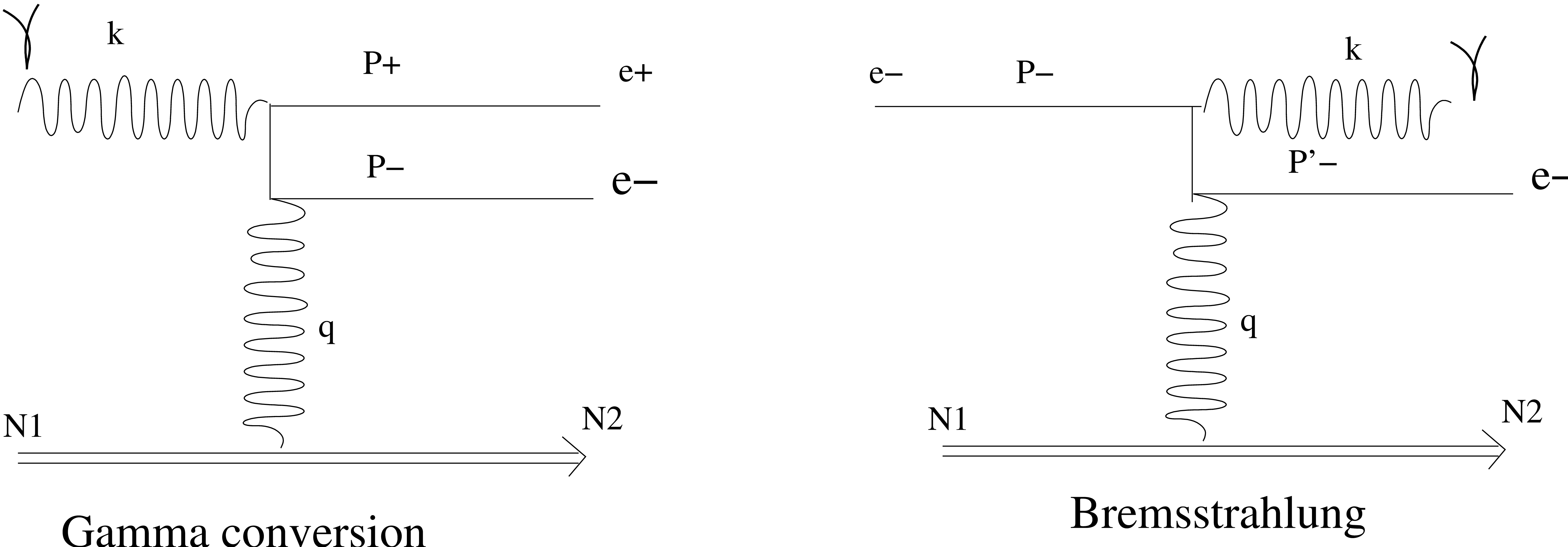
Fig. 54 Feynman diagrams of Gamma conversion and bremsstrahlung processes.

For both processes, the scattering can be formulated by:

\[\mathcal{K}_{1}(k_{1},{{\boldsymbol{\zeta}}}^{(1)}) + \mathcal{N}_{1}(k_{\mathcal {N}_{1}}, {{\boldsymbol{\zeta}}}^{(\mathcal {N}_{1})}) \longrightarrow \mathcal{P}_{1}(p_{1},{{\boldsymbol{\xi}}}^{(1)}) + \mathcal{P}_{2}(p_{2},{{\boldsymbol{\xi}}}^{(2)}) + \mathcal{N}_{2}(p_{\mathcal{N}_{2}}, {{\boldsymbol{\xi}}}^{(\mathcal{N}_{2})})\]

Where \(\mathcal{N}_{1}(k_{\mathcal {N}_{1}}, {{\boldsymbol{\zeta}}}^{(\mathcal {N}_{1})})\) and \(\mathcal{N}_{2}(p_{\mathcal{N}_{2}}, {{\boldsymbol{\xi}}}^{(\mathcal{N}_{2})})\) are the initial and final state of the field of the nucleus respectively assumed to be unchanged, at rest and unpolarized. This leads to \(k_{\mathcal {N}_{1}} = k_{\mathcal {N}_{2}} = 0\) and \({{\boldsymbol{\zeta}}}^{(\mathcal {N}_{1})} = {{\boldsymbol{\xi}}}^{(\mathcal{N}_{2})} = 0\).

In the case of gamma conversion process: \(\mathcal{K}_{1}(k_{1},{{\boldsymbol{\zeta}}}^{(1)})\) is the incoming photon initial state with momentum \(k_{1}\) and polarization state \({{\boldsymbol{\zeta}}}^{(1)}\). \(\mathcal{P}_{1}(p_{1},{{\boldsymbol{\xi}}}^{(1)})\) and \(\mathcal{P}_{2}(p_{2},{{\boldsymbol{\xi}}}^{(2)})\) are the two photons final states with momenta \(p_{1}\) and \(p_{2}\) and polarization states \({{\boldsymbol{\xi}}}^{(1)}\) and \({{\boldsymbol{\xi}}}^{(2)}\).

In the case of bremsstrahlung process: \(\mathcal{K}_{1}(k_{1},{{\boldsymbol{\zeta}}}^{(1)})\) is the incoming lepton \(e^{-}(e^{+})\) initial state with momentum \(k_{1}\) and polarization state \({{\boldsymbol{\zeta}}}^{(1)}\). \(\mathcal{P}_{1}(p_{1},{{\boldsymbol{\xi}}}^{(1)})\) is the lepton \(e^{-}(e^{+})\) final state with momentum \(p_{1}\) and polarization state \({{\boldsymbol{\xi}}}^{(1)}\). \(\mathcal{P}_{2}(p_{2},{{\boldsymbol{\xi}}}^{(2)})\) is the bremsstrahlung photon in final state with momentum \(p_{2}\) and polarization state \({{\boldsymbol{\xi}}}^{(2)}\).

Polarization transfer from the lepton e⁺e^- to a photon

The polarization transfer from an electron (positron) to a photon in a bremsstrahlung process was first calculated by Olsen and Maximon [OM59] taking into account both Coulomb and screening effects. In the Stokes vector formalism, the \(e^{-}(e^{+})\) polarization state can be transformed to a photon polarization finale state by means of interaction matrix \(T_{\gamma}^{b}\). It defined via

(191)\[\begin{split}\left(\begin{array}{c} O \\ {{\boldsymbol{\xi}}}^{(2)} \end{array}\right) = T_{\gamma}^{b} \, \left(\begin{array}{c} 1 \\ {{\boldsymbol{\zeta}}}^{(1)} \end{array}\right)\;,\end{split}\]

and

(192)\[\begin{split}T_{\gamma}^{b}\approx \left( \begin{array}{cccc} 1 & 0 & 0 & 0 \\ D & 0 & 0 & 0 \\ 0 & 0 & 0 & 0 \\ 0 & T & 0 & L \\ \end{array} \right)\;,\end{split}\]

where

(193)\[\begin{split}I &= (\epsilon_{1}^{2}+\epsilon_{2}^{2})(3+2\Gamma)-2\epsilon_{1}\epsilon_{2}(1+4u^{2}\hat\xi^{2}\Gamma)\\ D &= \left\lbrace 8\epsilon_{1}\epsilon_{2}u^{2}\hat\xi^{2}\Gamma \right\rbrace / I\\ T &= \left\lbrace -4k\epsilon_{2}\hat\xi(1-2\hat\xi)u \Gamma \right\rbrace / I \\ L &= k\lbrace(\epsilon_{1}+\epsilon_{2})(3+2\Gamma)-2\epsilon_{2}(1+4u^{2}\hat\xi^{2}\Gamma)\rbrace / I\end{split}\]

and

\(\epsilon_{1}\)	Total energy of the incoming lepton \(e^{+}(e^{-})\) in units \(mc^{2}\)
\(\epsilon_{2}\)	Total energy of the outgoing lepton \(e^{+}(e^{-})\) in units \(mc^{2}\)
\(k\)	\(=(\epsilon_{1}-\epsilon_{2})\), the energy of the bremsstrahlung photon in units of \(mc^{2}\)
\({{\boldsymbol{p}}}\)	Electron (positron) initial momentum in units \(mc\)
\({{\boldsymbol{k}}}\)	Bremsstrahlung photon momentum in units \(mc\)
\({{\boldsymbol{u}}}\)	Component of \({{\boldsymbol{p}}}\) perpendicular to \({{\boldsymbol{k}}}\) in units \(mc\) and \(u=\vert {{\boldsymbol{u}}} \vert \)
\(\hat\xi\)	\(= 1/(1+u^{2})\)

Coulomb and screening effects are contained in \(\Gamma\), defined as follows

\[\begin{split}\Gamma &= \ln\left(\frac{1}{\delta}\right)-2-f(Z)+ \mathcal{F}\left(\frac{\hat\xi}{\delta}\right) \quad \mbox{for } \Delta \le 120 \\ \Gamma &= \ln\left( \frac{111}{\hat\xi Z^{\frac{1}{3}}}\right)-2-f(z) \quad \mbox{for } \Delta \ge 120\end{split}\]

with

\[\Delta = \frac{12 Z^{\frac{1}{3}}\epsilon_{1}\epsilon_{2} \hat\xi}{121 k} \quad \mbox{with $Z$ the atomic number and } \delta = \frac{k}{2\epsilon_{1}\epsilon{2}}\]

\(f(Z)\) is the Coulomb correction term derived by Davies, Bethe and Maximon [eal54]. \(\mathcal{F}({\hat\xi}/{\delta})\) contains the screening effects and is zero for \(\Delta \le 0.5 \) (No screening effects). For \(0.5 \le \Delta \le 120 \) (intermediate screening) it is a slowly decreasing function. The \(\mathcal{F}({\hat\xi}/{\delta})\) values versus \(\Delta\) are given in Table 28 [KM59] and used with a linear interpolation in between.

The polarization vector of the incoming \(e^{-}(e^{+})\) must be rotated into the frame defined by the scattering plane (x-z-plane) and the direction of the outgoing photon (z-axis). The resulting polarization vector of the bremsstrahlung photon is also given in this frame.

Table 28 \(\mathcal{F}({\hat\xi}/{\delta})\) for intermediate values of the screening factor.

\(\Delta\)	\(-\mathcal{F}\left({\hat\xi}/{\delta}\right)\) | \(\Delta\)		\(-\mathcal{F}\left({\hat\xi}/{\delta}\right)\)
0.5	0.0145	40.0	2.00
1.0	0.0490	45.0	2.114
2.0	0.1400	50.0	2.216
4.0	0.3312	60.0	2.393
8.0	0.6758	70.0	2.545
15.0	1.126	80.0	2.676
20.0	1.367	90.0	2.793
25.0	1.564	100.0	2.897
30.0	1.731	120.0	3.078
35.0	1.875

Using Eq.(191) and the transfer matrix given by Eq.(192) the bremsstrahlung photon polarization state in the Stokes formalism [McM54][McM61] is given by

\[\begin{split}\xi^{(2)} = \left( \begin{array}{c} \xi_{1}^{(2)}\\ \xi_{2}^{(2)} \\ \xi_{3}^{(2)} \\ \end{array} \right) \approx \left( \begin{array}{c} D \\ 0 \\ \zeta_{1}^{(1)}L + \zeta_{2}^{(1)}T \\ \end{array} \right)\end{split}\]

Remaining polarization of the lepton after emitting a bremsstrahlung photon

The \(e^{-}(e^{+})\) polarization final state after emitting a bremsstrahlung photon can be calculated using the interaction matrix \(T_{l}^{b}\) which describes the lepton depolarization. The polarization vector for the outgoing \(e^{-}(e^{+})\) is not given by Olsen and Maximon. However, their results can be used to calculate the following transfer matrix [Flottmann93b][Hoo97].

(194)\[\begin{split}\left(\begin{array}{c} O \\ {{\boldsymbol{\xi}}}^{(1)} \end{array}\right) = T_{l}^{b} \, \left(\begin{array}{c} 1 \\ {{\boldsymbol{\zeta}}}^{(1)} \end{array}\right)\end{split}\]

(195)\[\begin{split}T_{l}^{b}\approx \left( \begin{array}{cccc} 1 & 0 & 0 & 0 \\ D & M & 0 & E \\ 0 & 0 & M & 0 \\ 0 & F & 0 & M+P \\ \end{array} \right)\end{split}\]

where

\[\begin{split}I &=(\epsilon_{1}^{2}+\epsilon_{2}^{2})(3+2\Gamma)-2\epsilon_{1}\epsilon_{2}(1+4u^{2}\hat\xi^{2}\Gamma)\\ F &= \epsilon_{2} \left\lbrace 4k\hat\xi u (1-2\hat\xi)\Gamma\right\rbrace /I \\ E &= \epsilon_{1} \left\lbrace 4k\hat\xi u (2\hat\xi-1)\Gamma \right\rbrace /I\\ M &= \left\lbrace 4k\epsilon_{1}\epsilon_{2}(1+\Gamma - 2 u^{2}\hat\xi^{2} \Gamma)\right\rbrace / I \\ P &= \left\lbrace k^{2} (1+8 \Gamma(\hat\xi - 0.5)^{2}\right\rbrace / I\end{split}\]

and

\(\epsilon_{1}\)	Total energy of the incoming \(e^{+}/e^{-}\) in units \(mc^{2}\)
\(\epsilon_{2}\)	Total energy of the outgoing \(e^{+}/e^{-}\) in units \(mc^{2}\)
\(k\)	\(=(\epsilon_{1}-\epsilon_{2})\), energy of the photon in units of \(mc^{2}\)
\({{\boldsymbol{p}}}\)	Electron (positron) initial momentum in units \(mc\)
\({{\boldsymbol{k}}}\)	Photon momentum in units \(mc\)
\({{\boldsymbol{u}}}\)	Component of \({{\boldsymbol{p}}}\) perpendicular to \({{\boldsymbol{k}}}\) in units \(mc\) and \(u=\vert {{\boldsymbol{u}}} \vert \)

Using Eq.(194) and the transfer matrix given by Eq.(195) the \(e^{-}(e^{+})\) polarization state after emitting a bremsstrahlung photon is given in the Stokes formalism by

\[\begin{split}\xi^{(1)} = \left( \begin{array}{c} \xi_{1}^{(1)}\\ \xi_{2}^{(1)} \\ \xi_{3}^{(1)} \\ \end{array} \right) \approx \left( \begin{array}{c} \zeta_{1}^{(1)} M + \zeta_{3}^{(1)} E \\ \zeta_{2}^{(1)} M \\ \zeta_{3}^{(1)}(M+P) + \zeta_{1}^{(1)} F \\ \end{array} \right) \;.\end{split}\]

Polarized Gamma conversion into an electron–positron pair

Method

The polarized version of gamma conversion is based on the EM standard process G4GammaConversion. Mean free path and the distribution of explicitly generated final state particles are treated by this version. For details consult Gamma Conversion into e+e- Pair.

The remaining task is to attribute polarization vectors to the generated final state leptons, which is discussed in the following.

Polarization transfer from the photon to the two leptons

Gamma conversion process is essentially the inverse process of bremsstrahlung and the interaction matrix is obtained by inverting the rows and columns of the bremsstrahlung matrix and changing the sign of \(\epsilon_{2}\), cf. Polarized Bremsstrahlung for electron and positron. It follows from the work by Olsen and Maximon [OM59] that the polarization state \(\xi^{(1)}\) of an electron or positron after pair production is obtained by

(196)\[\begin{split}\left(\begin{array}{c} O \\ {{\boldsymbol{\xi}}}^{(1)} \end{array}\right) = T_{l}^{p} \, \left(\begin{array}{c} 1 \\ {{\boldsymbol{\zeta}}}^{(1)} \end{array}\right)\end{split}\]

and

(197)\[\begin{split}T_{l}^{p}\approx \left( \begin{array}{cccc} 1 & D & 0 & 0 \\ 0 & 0 & 0 & T \\ 0 & 0 & 0 & 0 \\ 0 & 0 & 0 & L \\ \end{array} \right) \;,\end{split}\]

where

(198)\[\begin{split}I &= (\epsilon_{1}^{2}+\epsilon_{2}^{2})(3+2\Gamma)+2\epsilon_{1}\epsilon_{2}(1+4u^{2}\hat\xi^{2}\Gamma)\\ D &= \left\lbrace -8\epsilon_{1}\epsilon_{2}u^{2}\hat\xi^{2}\Gamma \right\rbrace / I\\ T &= \left\lbrace -4k\epsilon_{2}\hat\xi(1-2\hat\xi)u \Gamma \right\rbrace / I \\ L &= k\lbrace(\epsilon_{1}-\epsilon_{2})(3+2\Gamma)+2\epsilon_{2}(1+4u^{2}\hat\xi^{2}\Gamma)\rbrace/ I\end{split}\]

and

\(\epsilon_{1}\)	total energy of the first lepton \(e^{+}(e^{-})\) in units \(mc^{2}\)
\(\epsilon_{2}\)	total energy of the second lepton \(e^{-}(e^{+})\) in units \(mc^{2}\)
\(k=(\epsilon_{1}+\epsilon_{2})\)	energy of the incoming photon in units of \(mc^{2}\)
\({{\boldsymbol{p}}}\)	electron=positron initial momentum in units \(mc\)
\({{\boldsymbol{k}}}\)	photon momentum in units \(mc\)
\({{\boldsymbol{u}}}\)	electron/positron initial momentum in units \(mc\)
\(u\)	\(=\vert {{\boldsymbol{u}}} \vert \)

Coulomb and screening effects are contained in \(\Gamma\), defined in section Polarized Bremsstrahlung for electron and positron.

Using Eq.(196) and the transfer matrix given by Eq.(197) the polarization state of the produced \(e^{-}(e^{+})\) is given in the Stokes formalism by:

\[\begin{split}\xi^{(1)} = \left( \begin{array}{c} \xi_{1}^{(1)}\\ \xi_{2}^{(1)} \\ \xi_{3}^{(1)} \\ \end{array} \right) \approx \left( \begin{array}{c} \zeta_{3}^{(1)} T \\ 0 \\ \zeta_{3}^{(1)} L \\ \end{array} \right)\end{split}\]

Polarized Photoelectric Effect

Method

This section describes the basic formulas of polarization transfer in the photoelectric effect class (G4PolarizedPhotoElectricEffect). The photoelectric effect is the emission of electrons from matter upon the absorption of electromagnetic radiation, such as ultraviolet radiation or x-rays. The energy of the photon is completely absorbed by the electron and, if sufficient, the electron can escape from the material with a finite kinetic energy. A single photon can only eject a single electron, as the energy of one photon is only absorbed by one electron. The electrons that are emitted are often called photoelectrons. If the photon energy is higher than the binding energy the remaining energy is transferred to the electron as a kinetic energy

\[E_{kin}^{e^-} = k-B_{shell}\]

In Geant4 the photoelectric effect process is taken into account if:

\[k > B_{shell}\]

Where \(k\) is the incoming photon energy and \(B_{shell}\) the electron binding energy provided by the class G4AtomicShells.

The polarized version of the photoelectric effect is based on the EM standard process G4PhotoElectricEffect. Mean free path and the distribution of explicitly generated final state particles are treated by this version. For details consult section PhotoElectric Effect.

The remaining task is to attribute polarization vectors to the generated final state electron, which is discussed in the following.

Polarization transfer

The polarization state of an incoming polarized photon is described by the Stokes vector \(\vec{\zeta}^{(1)}\). The polarization transfer to the photoelectron can be described in the Stokes formalism using the same approach as for the bremsstrahlung and gamma conversion processes, cf. Polarized Bremsstrahlung for electron and positron and Polarized Gamma conversion into an electron–positron pair. The relation between the photoelectron’s Stokes parameters and the incoming photon’s Stokes parameters is described by the interaction matrix \(T_{l}^{p}\) derived from H. Olsen [OV58] and reviewed by H.W McMaster [McM61]:

(199)\[\begin{split}\left(\begin{array}{c} I^{\prime} \\ \vec{\xi}^{(1)} \end{array}\right) = T_{l}^{p} \, \left(\begin{array}{c} I_0 \\ \vec{\zeta}^{(1)} \end{array}\right)\end{split}\]

In general, for the photoelectric effect as a two-body scattering, the cross section should be correlated with the spin states of the incoming photon and the target electron. In our implementation the target electron is not polarized and only the polarization transfer from the photon to the photoelectron is taken into account. In this case the cross section of the process remains polarization independent. To compute the matrix elements we take advantage of the available kinematic variables provided by the generic G4PhotoelectricEffect class. To compute the photoelectron spin state (Stokes parameters), four main parameters are needed:

• The incoming photon Stokes vector \(\vec{\zeta}^{(1)}\)

• The incoming photon’s energy \(k\).

• the photoelectron’s kinetic energy \(E_{kin}^{e^-}\) or the Lorentz factors \(\beta\) and \(\gamma\).

• The photoelectron’s polar angle \(\theta\) or \(\cos\theta\).

The interaction matrix derived by H. Olsen [OV58] is given by:

(200)\[\begin{split}T_{l}^{P}= \left( \begin{array}{cccc} 1+D & -D & 0 & 0 \\ 0 & 0 & 0 & B \\ 0 & 0 & 0 & 0 \\ 0 & 0 & 0 & A \\ \end{array} \right)\end{split}\]

where

\[\begin{split}D &= \frac{1}{k}\left[\frac{2}{k\epsilon(1-\beta \cos\theta)}-1 \right]\\ A &= \frac{\epsilon}{\epsilon+1}\left[\frac{2}{k\epsilon}+\beta\cos\theta+\frac{2}{k\epsilon^2(1-\beta \cos\theta)}\right]\\ B &= \frac{\epsilon}{\epsilon+1}\beta\sin\theta\left[\frac{2}{k\epsilon(1-\beta \cos\theta)}-1\right]\end{split}\]

Using Eq.(199) and the transfer matrix given by Eq.(200) the polarization state of the produced \(e^{-}\) is given in the Stokes formalism by:

(201)\[\begin{split}\vec{\xi}^{(1)} = \left( \begin{array}{c} \xi_{1}^{(1)}\\ \xi_{2}^{(1)} \\ \xi_{3}^{(1)} \\ \end{array} \right) = \left( \begin{array}{c} \zeta_{3}^{(1)} B \\ 0 \\ \zeta_{3}^{(1)} A \\ \end{array} \right)\end{split}\]

From equation (201) one can see that a longitudinally (transversally) polarized photoelectron can only be produced if the incoming photon is circularly polarized.

Bibliography

aal

G. Alexander at al. Undulator-based production of polarized positrons: a proposal for the 50-gev beam in the fftb. Technical Report SLAC-TN-04-018, SLAC-PROPOSAL-E-166, SLAC.

eal54(1,2)

H. Davies et al. Theory of bremsstrahlung and pair production. ii. integral cross section for pair production. Phys. Rev., 93(4):788–795, 1954.

eal(1,2,3)

P. Starovoitov et al. in preparation.

eal85

R. Brun et al. The geant3 electromagnetic shower program and a comparison with the egs3 code. Technical Report CERN-DD/85/1, CERN, 1985.

Flottmann93a(1,2,3)

K. Flöttmann. DESY-93-161, DESY Hamburg, phd thesis edition, 1993.

Flottmann93b

K. Flöttmann. Investigations toward the development of polarized and unpolarized high intensity positron sources for linear colliders. Universitat Hamburg, phd thesis edition, 1993.

FM57

G. W. Ford and C. J. Mullin. Phys. Rev., 108:477, 1957.

Hoo97(1,2)

Johannes Marinus Hoogduin. Electron, positron and photon polarimetry. Rijksuniversiteit Groningen, phd thesis edition, 1997.

KM59(1,2)

H. W. Koch and J. W. Motz. Bremsstrahlung cross-section formulas and related data. Rev. Mod. Phys., 31(4):920–955, 1959.

Lai08

K. Laihem. Measurement of the positron polarization at an helical undulator based positron source for the International Linear Collider ILC. Humboldt University Berlin, Germany, phd thesis edition, 2008.

LT54a

F.W. Lipps and H.A. Tolhoek. Polarization phenomena of electrons and photons i. Physica, 20:85, 1954.

LT54b

F.W. Lipps and H.A. Tolhoek. Polarization phenomena of electrons and photons ii. Physica, 20:395, 1954.

LKNS

J. C. Liu, T. Kotseroglou, W. R. Nelson, and D. C. Schultz. Polarization study for nlc positron source using egs4. Technical Report SLAC-PUB-8477, SLAC.

McM61(1,2,3,4,5,6,7,8)

W. H. McMaster. Rev. Mod. Phys., 33():8, 1961.

McM54

W.H. McMaster. Polarization and the stokes parameters. American Journal of Physics, 22(6):351–362, 1954.

NBH93

Y. Namito, S. Ban, and H. Hirayama. Implementation of linearly polarized photon scattering into the egs4 code. Nucl. Instrum. Meth. A, 332:277, 1993.

NHR85

W.R. Nelson, H. Hirayama, and D.W.O. Rogers. EGS4 code system. SLAC, Dec 1985. SLAC-265, UC-32.

OM59(1,2)

H. Olsen and L.C. Maximon. Photon and electron polarization in high- energy bremsstrahlung and pair production with screening. Physical Review, 114:887–904, 1959.

OV58(1,2)

H. Olsen and Kgl. N. Videnskab. Selskabs Forh., 1958.

Pag57(1,2)

L. A. Page. Polarization effects in the two-quantum annihilation of positrons. Phys. Rev., 106:394–398, 1957.

Ste58

P. Stehle. Phys. Rev., 110:1458, 1958.

Sto52

G. Stokes. Trans. Cambridge Phil. Soc., 9 edition, 1852.

1

Note, for an incoming particle travelling on the \(Z\)-axis (of GRF), the \(y\)-axis of the PRF of both outgoing particles is parallel to the \(y\)-axis of the interaction frame.