Pair production by Linearly Polarized Gamma Rays - Livermore Model

A method to study the pair production interaction of linearly polarized gamma rays at energies 50 MeV was discussed in [DKT99]. The study of the differential cross section for pair production shows that the polarization information is coded in the azimuthal distribution of the electron - positron pair created by polarized photons (Fig. 55).

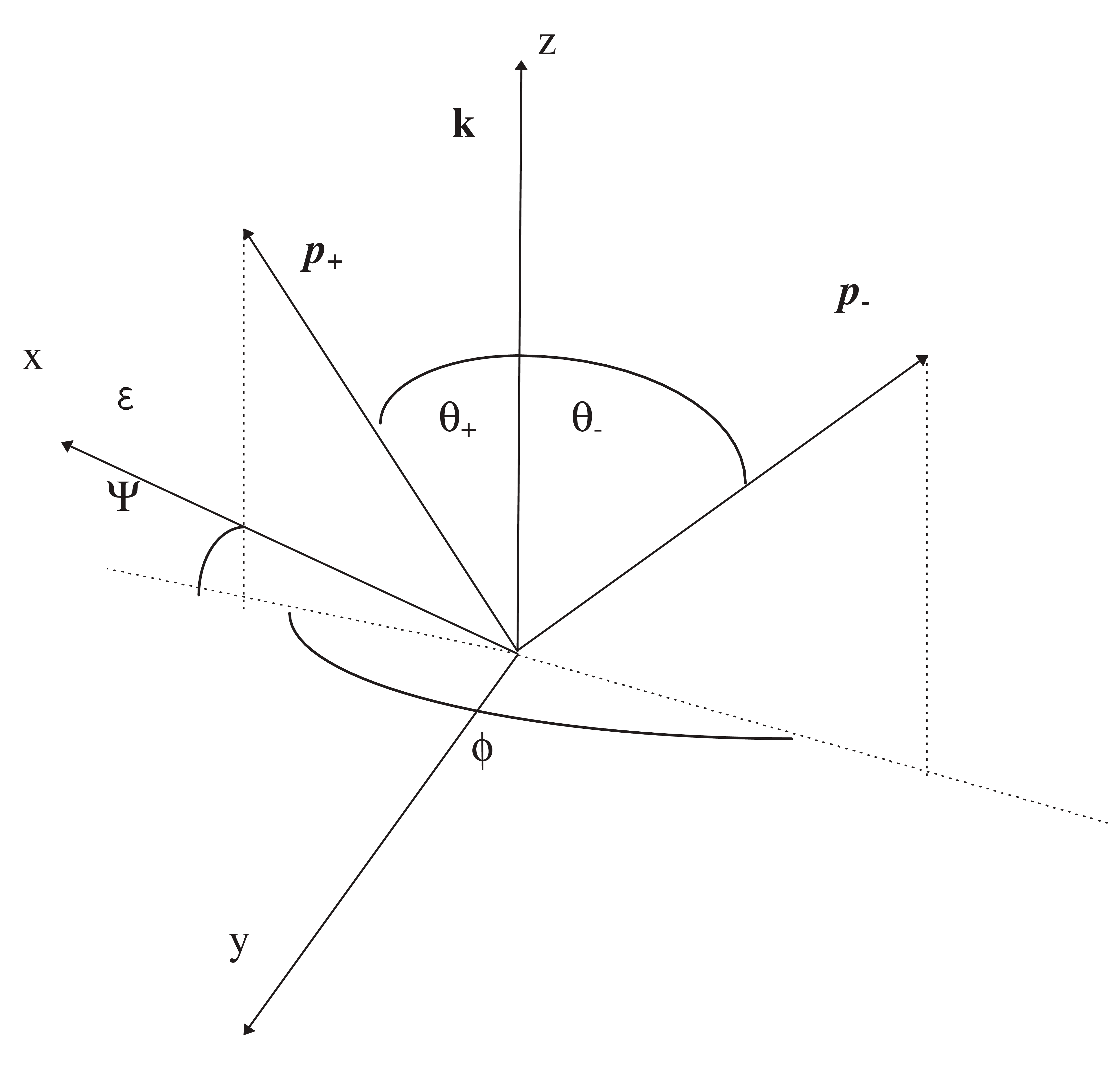
Fig. 55 Angles occurring in the pair creation

Relativistic cross section for linearly polarized gamma ray

The cross section for pair production by linearly polarized gamma rays in the high energy limit using natural units with \(h/2\pi =c=1\) is

\[\begin{split}d\sigma & = \frac{-2 \alpha Z^2r_0m^2}{(2 \pi)^2 \omega ^3} dE d\Omega_{+} d\Omega_{-} \frac{E(\omega - E)}{\lvert \vec{q}\rvert^4} \left\{ 4 \left[ E \frac{\sin{\theta _-} \cos{\Psi}}{1-\cos{\theta _-}} + (\omega - E) \frac{\sin{\theta _+} \cos{(\Psi + \phi)}} {1- \cos{\theta _+}} \right] ^2 \right. \\ &- \lvert \vec{q}\rvert^2 \left[ \frac{\sin{\theta _-}\cos{\Psi}}{1-\cos{\theta _-}} - \frac{\sin{\theta _+ \cos{(\Psi + \phi)}}}{1- \cos{\theta _+}} \right] ^2 \\ &- \left. \omega ^2 \frac{\sin{\theta _-} \sin{\theta _+}}{(1-\cos{\theta_{-}})(1- \cos{\theta _+})} \left[ \frac{E\sin{\theta _+}}{(\omega _ E)\sin{\theta _-}} + \frac{(\omega - E)\sin{\theta_{-}}}{E \sin{\theta _+}} + 2\cos{\phi} \right] \right\} \; ,\end{split}\]

with

\[\begin{split}\lvert \vec{q}\rvert^2 & = -2 \left[ E(\omega - E)(1 - \sin{\theta _+} \sin{\theta _-} \cos{\phi} - \cos{\theta _+} \cos{\theta _-}) \right. \\ & \left. + \omega E(\cos{\theta _+}-1) + \omega (\omega - E)(cos{\theta _-}-1) + m^2 \right] \; .\end{split}\]

\(E\) is the positron energy and we have assumed that the polarization direction is along the \(x\) axis (see Fig. 55).

Spatial azimuthal distribution

Integrating this cross section over energy and polar angles yields the spatial azimuthal distribution, that was calculated in [DKT99] using a Monte Carlo procedure.

Fig. 56 shows an example of this distribution for 100 MeV gamma-ray. In this figure the range of the \(\phi\) axis is restricted between 3.0 and \(\pi\) since it gives the most interesting part of the distribution. For angles smaller than 3.0 this distribution monotonically decreases to zero.

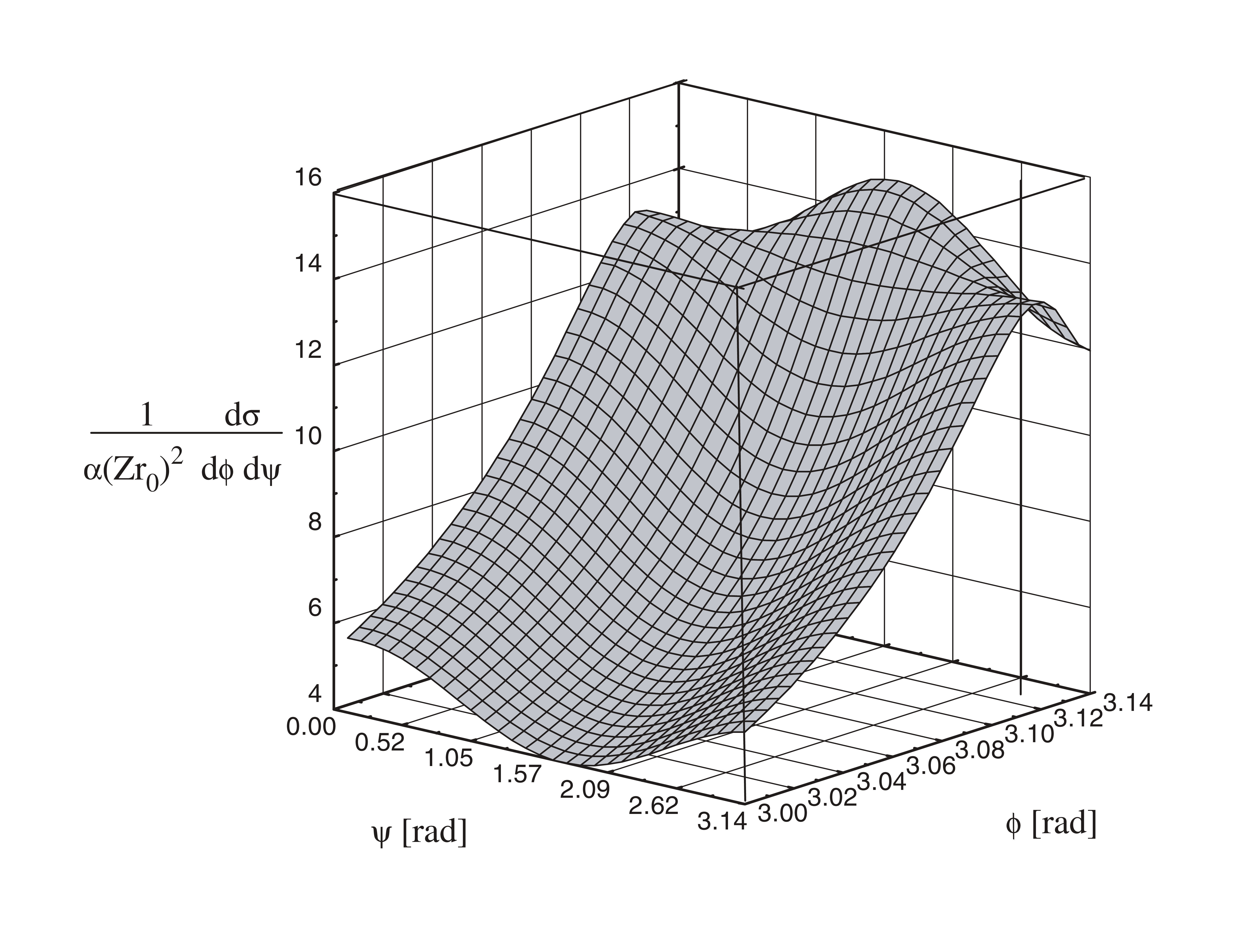
Fig. 56 Spatial azimuthal distribution of a pair created by 100 MeV photon

In Geant4 the azimuthal distribution surface is parametrized in terms of smooth functions of \((\phi , \psi )\) .

\[f(\phi ,\psi ) = f_{\pi /2}(\phi ) \sin ^2 \psi + f_0 (\phi) \cos ^2 \psi \; .\]

Since both \(f_0 (\phi)\) and \(f_{\pi /2} (\phi)\) are functions that rapidly vary when \(\phi\) approaches \(\pi\), it was necessary to adjust the functions in two ranges of \(\phi\):

\(0 \leq \phi \leq 3.05\) rad.
\(3.06\) rad \(\leq \phi \leq \pi\) ,

whereas in the small range \(3.05 \leq \phi \leq 3.06\) we extrapolate the two fitting functions until the intersection point is reached.

In region 2 we used Lorentzian functions of the form

\[f(\phi ) = y_0 + \frac{2A \omega}{\pi [\omega ^2 + 4 (\phi - x_c)^2]} \; ,\]

whereas for region 1 the best fitting function was found to adopt the form:

\[f(\phi ) = a + d \tan{(b \phi + c)} \; .\]

The paper [DKT99] reports the coefficients obtained in different energy regions to fit the angular distribution and their function form as function of gamma-ray as energy reported in the Table 30 and Table 31 below.

Table 30 Fit for the parameter of \(f_0 (\phi )\) function.
Parameter	Function	a	b	c
\(y_0\)	\(a\ln{E} - b\)	\(2.98 \pm 0.06\)	\(7.7 \pm 0.4\)	–
\(A\)	\(a\ln{E} - b\)	\(1.41 \pm 0.08\)	\(5.6 \pm 0.5\)	–
\(\omega\)	\(a + b/E + c/E^3\)	\(0.015 \pm 0.001\)	\(9.5 \pm 0.6\)	\((-2.2 \pm 0.1) 10^4\)
\(x_c\)	\(a + b/E + c/E^3\)	\(3.143 \pm 0.001\)	\(-2.7 \pm 0.2\)	\((2 \pm 1)10^3\)

Table 31 Fit for the parameter of \(f_{\pi /2} (\phi)\) function.
Parameter	Function	a	b	c
\(y_0\)	\(a\ln{E} - b\)	\(1.85 \pm 0.07\)	\(5.1 \pm 0.4\)	–
\(A\)	\(a\ln{E} - b\)	\(1.3 \pm 0.1\)	\((6.6 \pm 0.2)10^{-3}\)	–
\(\omega\)	\(a + b/E + c/E^3\)	\(0.008 \pm 0.002\)	\(12.1 \pm 0.9\)	\((-2.8 \pm 0.8) 10^4\)
\(x_c\)	\(3.149\)	–	–	–

Unpolarized Photons

A special treatment is devoted to unpolarized photons. In this case a random polarization in the plane perpendicular to the incident photon is selected.

Bibliography

DKT99(1,2,3,4): G.O. Depaola, C.N. Kozameh, and M.H. Tiglio. A method to determine the polarization of high energy gamma rays. Astroparticle Physics, 10():175, 1999.