(top left) The LHCb VELO vacuum tank. The cut-away view allows the VELO sensors, hybrids and module support on the left-hand side to be seen. (top right) A photograph of one side of the VELO during assembly showing the silicon sensors and readout hybrids. (bottom) Cross-section in the $xz$ plane at $y=0$ of the sensors and a view of the sensors in the $xy$ plane. The detector is shown in its closed position. $R$ ($\Phi$ ) sensors are shown with solid blue (dashed red) lines. The modules at positive (negative) $x$ are known as the left or A-side (right or C-side).

Schematic representation of an $R$ and a $\Phi$ sensor. The $R$ sensor strips are arranged into four approximately $45 ^{\circ} $ segments and have routing lines perpendicular to the strips. The $\Phi$ sensor has two zones with inner and outer strips. The routing lines of the inner strips are orientated parallel to the outer strips.

Illustration of the influence of the proton beams on the beam volume pressure. The readings of the beam volume (PE 412) and detector volume (PE 422) are shown, and the increase in pressure in the beam volume coinciding with the beam injections (each containing $2\times10^{14}$ protons) at $t = 6 \mathrm{hours}$ can be seen. The beams were dumped 24 hours later.

The horizontal position of LHC collision vertices as reconstructed by the A-Side (left) and C-Side (right). These online screenshots of data illustrate the "stop-measure-move" cycle of the closing procedure, where each peak in the distribution corresponds to a "stop", as well as the degradation of vertex resolution with opening distance.

(left) Material passed through on trajectories originating from the interaction point and terminating at the radius of the first active strip in the detector expressed in terms of the fraction of a radiation length ( $ X_0$ ) and as a function of pseudorapidity ($\eta$) and azimuthal angle ($\phi$). The material is higher in the regions around $\pm90 ^{\circ} $ where the two halves of the detector overlap. (right) Breakdown of the total material budget by component of the VELO . The number given for each component is the percentage of the total average VELO material budget ($0.227 X_0 $).

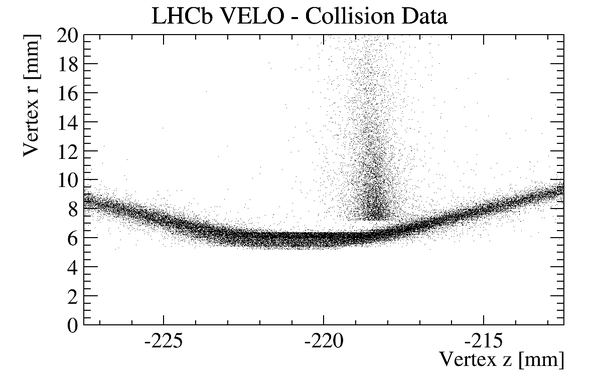
Vertices of hadronic interactions in the LHCb VELO material. (top left) Full VELO system with entrance and exit regions visible in data. (top right) Zoom in to a group of sensors downstream from the interaction point in data. (bottom left) the same region reconstructed using simulation events. (bottom right) Zoom onto an pile-up module consisting of a single R-sensor to check the distance between the sensor and foil.

An example of the scan over the digitisation phases (see text). Data for 16 analogue links are shown. The horizontal axis represents the sampling time, where the integer numbers indicate the location of the serially transmitted Beetle channels, and between two channels there are 16 bins. The solid red vertical line indicates the chosen sampling point and the dashed red lines the position of the previous and next samples.

The FHS distribution before and after the first gain calibration. The data were taken two months apart in late 2009. One entry is made in the histogram for each link.

Pulse-shape obtained by combining data from all sensors, with a 1 $ {\rm ns}$ time step and after applying for each sensor the time shift determined by the procedure. The plot on the left shows the ADC spectra versus time. The plot on the right shows the most probable value for each time bin obtained from a fit of a Landau convolved with a Gaussian function. A bifurcated Gaussian function is fitted to this distribution from which the rise and the fall widths are obtained. The fitted function also predicts the amount of pre-spill (25 $ {\rm ns}$ before the chosen point) and the spillover (25 ns after), which are marked with red vertical dotted lines. The chosen sampling time is also marked with a red vertical dotted line.

Typical raw (Non-Zero Suppressed) data ADC values. Data from two ASICs, each with four analogue links, is shown. Variations in the pedestal values at the ASIC, analogue link, and channel level are seen.

Distribution of common mode noise per link. The blue histogram is for all links. The green histogram is for links in a ASIC that has large signals (see text).

(left) Event snapshot for an ASIC that has large signals (channels 1024-1152). The blue dots are the raw ADC values. The red lines are the pedestals. (right) ASIC baseline shift in response to injected charge in units of the most probable charge deposited by a MIP in 300 $ \upmu\rm m$ thick silicon.

Example of the graphical user interface used in the VELO monitoring. Shown are distributions of the number of hits per VELO track segment (top left), the track angle with respect to the beam axis (top right), and the ADC counts of $R$ and $\Phi$ sensor clusters associated to a track (bottom left and right, respectively). The results of the current run are shown in red filled symbols and the reference data for comparison are shown as black open symbols.

(left) Fit of the signal distribution for Sensor 104 (a $\Phi$ sensor) for clusters on long tracks with a track intercept point on the sensor $10 < r (\rm mm ) <15$. (right) The most probable value of the fits to sensors 40 and 104, the $R$ and $\Phi$ sensor of the same module respectively, as a function of the track intercept point radius. The cluster ADC counts were normalised to a track crossing 300 $ \upmu\rm m$ of silicon.

Noise in ADC counts averaged across the 42 installed R (left) and $\Phi$ (right) sensors, with the error bars indicating the RMS of the distribution.

Signal to noise (S/N) ratio from the MPV of the signal for single strip clusters on tracks divided by the noise of that strip. Shown are the S/N values for sensor 40 (R) and sensor 104, the $\Phi$ sensor of the same module, as a function of impact point radius.

(left) The VELO resolution for two projected angle bins for the $R$ sensors as a function of the readout pitch compared with binary resolution. (right) Resolution divided by pitch as function of the track projected angle for four different strip pitches.

The percentage of one (left) and two (right) strip clusters as a function of the track projected angle for four different strip pitches.

Cluster occupancy in the VELO silicon strip detectors. (left plots) Average occupancy in the sensor as a function of the position of the sensor along the beam-line. (right plots) Occupancy as a function of the local radius of strips on the $R$ sensors, with a negative sign applied to sensors on one half. The upper plots show the occupancy when fully closed using 2011 data with a $\mu$ of 1.7 and for events selected using a random trigger or with events passing the high level trigger. The lower plots show the occupancy as a function of closing distance with fully closed labelled as 0 $\rm mm$ , the points below then follow in order of the retraction distance indicated in the key.

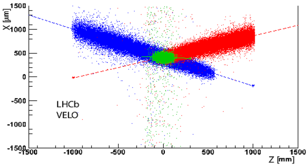
(left) Imaging of the LHC beams through the reconstruction of the production vertex of tracks in 2010. The vertices from beam-gas interactions with the beam travelling in the $+z$ ($-z$) direction in LHCb are shown in blue (red). Vertices arising from beam-beam interactions are in green. The vertical axis represents the horizontal direction ($x$) and the horizontal axis the beam direction ($z$). (right) An event display image showing clusters in $R$ and $\Phi$ sensors with a high occupancy in a localised region assumed to be due to a beam background splash event.

The cluster finding efficiency for each sensor with all strips (left) and when identified bad strips are excluded (right).

The intercept position of an extrapolated track when a cluster is not found for two example $R$ (left) and $\Phi$ (right) sensors. The bad channels are clearly visible.

Currents measured for each sensor as a function of time (bottom). The integrated luminosity delivered to LHCb and the average sensor temperature is shown over the same time scale (middle and top). Increases in the delivered luminosity are matched by increases in the sensor currents. The evolution of the mean measured current agrees well with the prediction from simulation. The mean measured value excludes sensors that are surface-current dominated.

The effective depletion voltage versus fluence for all VELO sensors up to 3.4 $ fb^{-1}$ delivered integrated luminosity.

Tracking efficiency for the 2011 data and simulation for the VELO as a function of the momentum, p (top left), the pseudorapidity, $\eta$ (top right), the azimuthal angle $\phi$ (bottom left) and the total number of tracks in the event, $N_{track}$ (bottom right). The simulation has been reweighted to the number of tracks observed in data for the p,$\eta$ and $\phi$ plots. The error bars indicate the statistical uncertainty.

(left) Fraction of ghost tracks versus number of VELO clusters in simulation. (right) VELO pattern recognition timing versus number of clusters, the pattern recognition alone (magenta triangles), the raw data decoding (blue squares) and the combined (red circles) timings are shown. The times are scaled to a 2.8 $ {\rm GHz}$ Xeon processor.

Example unbiased sensor residuals as a function of the $\phi$ coordinate using only the survey information (left) and using the track-based software alignment (right). Results are given for two different example sensors. (top) A significant improvement in the residuals is seen in this sensor with the track-based alignment. (bottom) In this sensor the alignment quality using the survey information is already good.

Misalignment between the two VELO halves in each run, evaluated by fitting the PV separately with tracks in the two halves of the VELO . The run numbers shown here span the period of the last four months of operations in 2010.

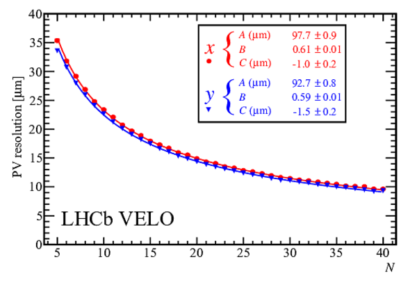
PV Resolution of events with exactly one PV in 2011 data as a function of track multiplicity. (left) $x$ (red) and $y$ (blue) resolution and (right) $z$ resolution. The fit parameters $A$, $B$ and $C$ for each coordinate are given.

$IP_x$ and $IP_y$ resolution as a function of momentum (left) and $IP_x$ as a function of $1/p_T$ and compared with simulation (right). Determined with 2012 data.

$IP_x$ resolution as a function of azimuthal angle $\phi$, measured on 2011 data and compared to simulation.

Decay time (left) and decay length (right) distribution for fake, prompt $ B ^0_s \rightarrow { J \mskip -3mu/\mskip -2mu\psi \mskip 2mu} \phi\rightarrow \mu ^+\mu ^- K ^+ K ^- $ candidates in 2011 data (black points) and simulation (solid red histogram). Only events with a single PV are used. The simulated data are generated inclusive $ { J \mskip -3mu/\mskip -2mu\psi \mskip 2mu} $ events from which signal $ B ^0_s \rightarrow { J \mskip -3mu/\mskip -2mu\psi \mskip 2mu} \phi$ are removed. In the data contributions from non- $ { J \mskip -3mu/\mskip -2mu\psi \mskip 2mu}$ {} di-muon combinations and from true $ B ^0_s \rightarrow { J \mskip -3mu/\mskip -2mu\psi \mskip 2mu} \phi$ are subtracted using the sPlot technique \cite{Pivk:2004ty}.

Decay time resolution (points) as a function of momentum (left) and as a function of the estimated decay time uncertainty (right) of fake, prompt $ B ^0_s \rightarrow { J \mskip -3mu/\mskip -2mu\psi \mskip 2mu} \phi\rightarrow \mu ^+\mu ^- K ^+ K ^- $ candidates in data. Only events with a single PV are used. Contributions from non- $ { J \mskip -3mu/\mskip -2mu\psi \mskip 2mu}$ {} di-muon combinations and from true $ B ^0_s \rightarrow { J \mskip -3mu/\mskip -2mu\psi \mskip 2mu} \phi$ are subtracted using the sPlot\ technique. The superimposed histogram shows the distribution of momentum (left) and estimated decay time uncertainty (right) on an arbitrary scale.

Animated gif made out of all figures.

Fraction of faulty strips classified as dead or noisy. The results are obtained from the methods used at production, occupancy spectrum studies, and a cluster finding efficiency analysis. Values are given at the time of production or start of operations in 2010, at the end of 2011, and at the end of 2012.