Distribution of $\overline{ D }{} {}^0$ candidate invariant mass for $ B ^0_ s $ candidates in the signal region defined in Sec. 4. Here the selection criteria have been modified to avoid biasing the distribution: the $\overline{ D }{} {}^0 $ candidate invariant mass requirement has been removed, and the $\chi^2 $ of the kinematic fit is calculated without applying the $\overline{ D }{} {}^0 $ mass constraint.

Result of the fit to the $ B ^0_ s \rightarrow \overline{ D }{} {}^0 K ^- \pi ^+ $ candidates invariant mass distribution shown with (a) linear and (b) logarithmic $y$-axis scales. Data points are shown in black, the total fit as a solid blue line and the components as detailed in the legend.

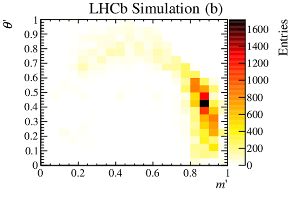
Distribution of $ B ^0_ s \rightarrow \overline{ D }{} {}^0 K ^- \pi ^+ $ candidates in the signal region over (a) the Dalitz plot and (b) the square Dalitz plot defined in Eq. (19). The effect of the $ D ^0$ veto can be seen as an unpopulated horizontal (curved) band in the (square) Dalitz plot.

SDP distributions of the background contributions from (a) combinatorial, (b) $\overline{\Lambda} {}^0_ b \rightarrow \overline{ D }{} {}^{(*)0} \overline p \pi ^+ $ and (c) $ B ^0 \rightarrow \overline{ D }{} {}^{(*)0} \pi ^+ \pi ^- $ backgrounds.

Signal efficiency across the SDP for (a) events triggered by signal decay products and (b) the rest of the event. The relative uncertainty at each point is typically $5 \%$. The effect of the $ D ^0$ veto can be seen as a curved band running across the SDP, while the $ D ^*$ veto appears in the bottom left corner of the SDP.

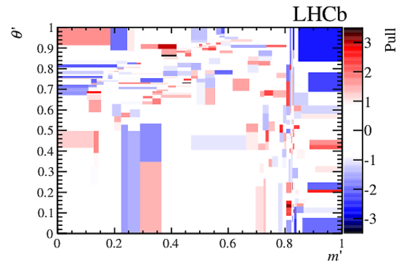
Distribution of the pull between data and the fit result as a function of SDP position.

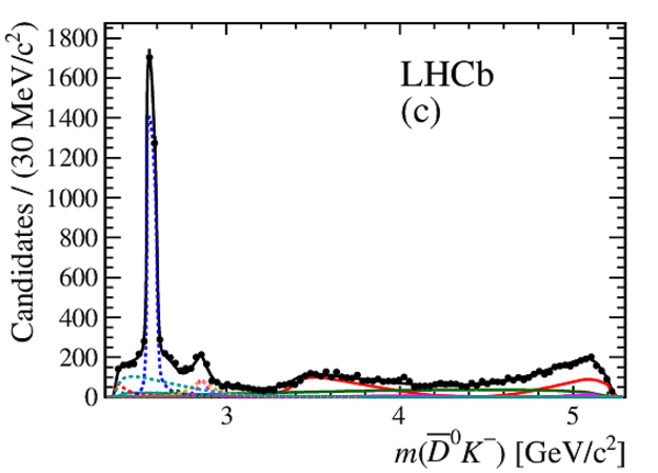
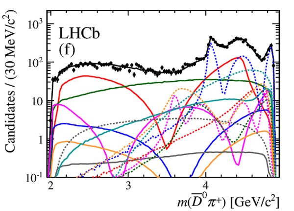
Projections of the data and the Dalitz plot fit result onto (a) $m( K ^- \pi ^+ )$, (c) $m(\overline{ D }{} {}^0 K ^- )$ and (e) $m(\overline{ D }{} {}^0 \pi ^+ )$, with the same projections shown with a logarithmic $y$-axis scale in (b), (d) and (f), respectively. The components are as described in the legend (small background components are not shown).

Projections of the data and the Dalitz plot fit result onto (a) $m( K ^- \pi ^+ )$ in the range $0.5$--$1.8 {\mathrm{ Ge V /}c^2} $, (b) $m(\overline{ D }{} {}^0 K ^- )$ between $2.2 {\mathrm{ Ge V /}c^2} $ and $3.2 {\mathrm{ Ge V /}c^2} $, (c) $m(\overline{ D }{} {}^0 K ^- )$ around the $D^{*}_{s2}(2573)^-$ resonance and (d) the $D^{*}_{sJ}(2860)^-$ region. Discrepancies between the data and the model are discussed at the end of Sec. 7. The components are as described in the legend for Fig 7.

Projections of the data and the Dalitz plot fit result onto the cosine of the helicity angle of the $ K ^- \pi ^+ $ system, $\cos\theta( K ^- \pi ^+ )$, for $m( K ^- \pi ^+ )$ slices of (a) $0$--$0.8 {\mathrm{ Ge V /}c^2} $, (b) $0.8$--$1.0 {\mathrm{ Ge V /}c^2} $, (c) $1.0$--$1.3 {\mathrm{ Ge V /}c^2} $ and (d) $1.4$--$1.5 {\mathrm{ Ge V /}c^2} $. The data are shown as black points, the total fit result as a solid blue curve, and the small contributions from $ B ^0 \rightarrow \overline{ D }{} {}^{(*)0} \pi ^+ \pi ^- $, $\overline{\Lambda} {}^0_ b \rightarrow \overline{ D }{} {}^{(*)0} \overline p \pi ^+ $ and combinatorial background shown as green, black and red curves, respectively.

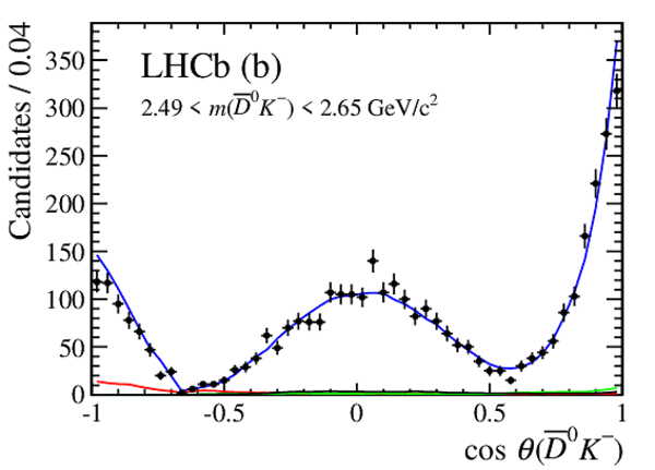
Projections of the data and the Dalitz plot fit result onto the cosine of the helicity angle of the $\overline{ D }{} {}^0 K ^- $ system, $\cos\theta(\overline{ D }{} {}^0 K ^- )$, for $m(\overline{ D }{} {}^0 K ^- )$ slices of (a) $0$--$2.49 {\mathrm{ Ge V /}c^2} $, (b) $2.49$--$2.65 {\mathrm{ Ge V /}c^2} $, (c) $2.65$--$2.77 {\mathrm{ Ge V /}c^2} $ and (d) $2.77$--$2.91 {\mathrm{ Ge V /}c^2} $. The data are shown as black points, the total fit result as a solid blue curve, and the small contributions from $ B ^0 \rightarrow \overline{ D }{} {}^{(*)0} \pi ^+ \pi ^- $, $\overline{\Lambda} {}^0_ b \rightarrow \overline{ D }{} {}^{(*)0} \overline p \pi ^+ $ and combinatorial background shown as green, black and red curves, respectively.

Projections of the data and Dalitz plot fit results with alternative models onto the cosine of the helicity angle of the $\overline{ D }{} {}^0 K ^- $ system, $\cos\theta(\overline{ D }{} {}^0 K ^- )$, for $2.49 < m(\overline{ D }{} {}^0 K ^- ) < 2.65 {\mathrm{ Ge V /}c^2} $. The data are shown as black points, the result of the baseline fit with a spin-2 resonance is given as a solid blue curve, and the result of the fit from the best model with a spin-0 resonance is shown as a dashed red line.

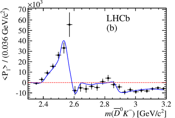
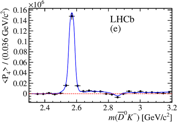
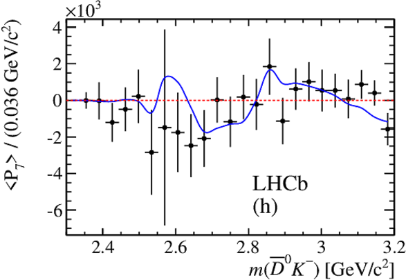
Legendre moments up to order 7 calculated as a function of $m(\overline{ D }{} {}^0 K ^- )$ for data (black data points) and the fit result (solid blue curve).

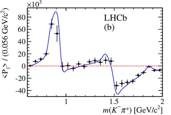
Legendre moments up to order 7 calculated as a function of $m( K ^- \pi ^+ )$ for data (black data points) and the fit result (solid blue curve).

Projections of the data and Dalitz plot fit results with alternative models onto the cosine of the helicity angle of the $\overline{ D }{} {}^0 K ^- $ system, $\cos\theta(\overline{ D }{} {}^0 K ^- )$, for $2.77 < m(\overline{ D }{} {}^0 K ^- ) < 2.91 {\mathrm{ Ge V /}c^2} $. The data are shown as black points, the result of the baseline fit with both spin-1 and spin-3 resonances is given as a solid blue curve, and results of fits from the best models with only either a spin-1 or a spin-3 resonance are shown as dashed red and dotted green lines, respectively. The dip at $\cos\theta(\overline{ D }{} {}^0 K ^- ) \approx -0.6$ is due to the $\overline{ D }{} {}^0 $ veto. Comparison of the data and the different fit results in the 50 bins of this projection gives $\chi^2 $ values of 47.3, 214.0 and 150.0 for the default, spin-1 only and spin-3 only models, respectively.

Fits of $\chi^2$ functions to the $2\Delta{\rm NLL}$ distributions obtained from fits to pseudoexperiments generated with (left) no $D_{s1}^*(2860)^-$ and (right) no $D_{s3}^*(2860)^-$ component. The corresponding $2\Delta{\rm NLL}$ values observed in data are 273 and 314, respectively (see Table 7).

Animated gif made out of all figures.

Excited charm-strange states above the $D_{s2}^*(2573)^-$ seen in $ D ^{(*)} K $ spectra by BaBar [5] in $ e ^+ e ^-$ collisions and by LHCb [6] in $pp$ collisions. Units of $ {\mathrm{ Me V /}c^2} $ are implied. The first source of uncertainty is statistical and the second is systematic.

Results of the $ B ^0_ s \rightarrow \overline{ D }{} {}^0 K ^- \pi ^+ $ candidate invariant mass fit. Uncertainties are statistical only.

Yields of the fit components within the signal region used for the Dalitz plot analysis.

Contributions to the fit model. Resonances labelled with subscript $v$ are virtual. Parameters and uncertainties are taken from Ref. [3] except where indicated otherwise. Details of these models are given in Sec. 5.

Fit fractions and complex coefficients determined from the Dalitz plot fit. Uncertainties are statistical only and are obtained as described in the text.

Resonance parameters of the $D^{*}_{s2}(2573)^-$, $D^{*}_{s1}(2860)^-$ and $D^{*}_{s3}(2860)^-$ states from the Dalitz plot fit (statistical uncertainties only).

Changes in NLL from fits with different hypotheses for the state(s) at $m(\overline{ D }{} {}^0 K ^- )=2860 {\mathrm{ Me V /}c^2} $. Units of $ {\mathrm{ Me V /}c^2} $ are implied for the masses and widths. When two pairs of mass and width values are given, the first corresponds to the lower spin state. Values marked * are discussed further in the text. There are two entries for spin-2 because two solutions were found.

Experimental systematic uncertainties on the fit fractions and complex amplitudes.

Breakdown of experimental systematic uncertainties on the fit fractions (%). The columns give the contributions from the different sources described in the text.

Breakdown of experimental systematic uncertainties on the masses and widths. Units of $ {\mathrm{ Me V /}c^2}$ are implied. The columns give the contributions from the different sources described in the text.

Model uncertainties on the fit fractions and complex amplitudes.

Breakdown of model uncertainties on the fit fractions (%). The columns give the contributions from the different sources described in the text.

Breakdown of model uncertainties on the masses and widths. Units of $ {\mathrm{ Me V /}c^2}$ are implied. The columns give the contributions from the different sources described in the text.

Results for the complex amplitudes and their uncertainties. The three quoted errors are statistical, experimental systematic and model uncertainties, respectively. The central values and statistical uncertainties are as reported in Table 5, while the experimental and model systematic uncertainties are as reported in Tables 8 and 11.

Results for the fit fractions and their uncertainties (%). The three quoted errors are statistical, experimental systematic and model uncertainties, respectively. Upper limits at both 90 % and 95 % confidence level (CL) are given for components that are not significant. The central values and statistical uncertainties are as reported in Table 5, while the experimental and model systematic uncertainties are as reported in Tables 8 and 11.

Results for the product branching fractions (top) ${\cal B}( B ^0_ s \rightarrow \overline{ D }{} {}^0 \overline{ K }{} {}^{*0} )\times{\cal B}(\overline{ K }{} {}^{*0} \rightarrow K ^- \pi ^+ )$ and (bottom) ${\cal B}( B ^0_ s \rightarrow D_s^{*-}\pi ^+ )\times{\cal B}(D_s^{*-} \rightarrow \overline{ D }{} {}^0 K ^- )$, for each $\overline{ K }{} {}^{*0} $ and $D_s^{*-}$ resonance. For the $\overline{ K }{} {}^{*0} $ resonances, where ${\cal B}(\overline{ K }{} {}^{*0} \rightarrow K ^- \pi ^+ )$ is known [3], the $ B ^0_ s $ decay branching fraction is also given. The four quoted uncertainties are statistical, experimental systematic, model and PDG uncertainties, respectively. Upper limits are given at 90 % (95 %) confidence level.

Interference fit fractions (%) from the nominal Dalitz plot fit. The amplitudes are: ($A_{0}$) $\overline{ K }{} {}^* (892)^{0}$, ($A_{1}$) $\overline{ K }{} {}^* (1410)^{0}$, ($A_{2}$) $\overline{ K }{} {}^*_0 (1430)^{0}$, ($A_{3}$) LASS nonresonant, ($A_{4}$) $\overline{ K }{} {}^*_2 (1430)^{0}$, ($A_{5}$) $\overline{ K }{} {}^* (1680)^{0}$, ($A_{6}$) $\overline{ K }{} {}^*_0 (1950)^{0}$, ($A_{7}$) $D^{*-}_{s v}$, ($A_{8}$) $D^{*}_{s0 v}(2317)^-$, ($A_{9}$) $D^{*}_{s2}(2573)^-$, ($A_{10}$) $D^{*}_{s1}(2700)^-$, ($A_{11}$) $D^{*}_{s3}(2860)^-$, ($A_{12}$) $D^{*}_{s1}(2860)^-$, ($A_{13}$) $B^{*+}_{v}$, ($A_{14}$) Nonresonant. The diagonal elements correspond to the fit fractions shown in Table 5.

Absolute statistical uncertainties on the interference fit fractions (%) from the Dalitz plot fit. The amplitudes are: ($A_{0}$) $\overline{ K }{} {}^* (892)^{0}$, ($A_{1}$) $\overline{ K }{} {}^* (1410)^{0}$, ($A_{2}$) $\overline{ K }{} {}^*_0 (1430)^{0}$, ($A_{3}$) LASS nonresonant, ($A_{4}$) $\overline{ K }{} {}^*_2 (1430)^{0}$, ($A_{5}$) $\overline{ K }{} {}^* (1680)^{0}$, ($A_{6}$) $\overline{ K }{} {}^*_0 (1950)^{0}$, ($A_{7}$) $D^{*-}_{s v}$, ($A_{8}$) $D^{*}_{s0 v}(2317)^-$, ($A_{9}$) $D^{*}_{s2}(2573)^-$, ($A_{10}$) $D^{*}_{s1}(2700)^-$, ($A_{11}$) $D^{*}_{s3}(2860)^-$, ($A_{12}$) $D^{*}_{s1}(2860)^-$, ($A_{13}$) $B^{*+}_{v}$, ($A_{14}$) Nonresonant. The diagonal elements correspond to the statistical uncertainties on the fit fractions shown in Table 5.

Absolute experimental systematic uncertainties on the interference fit fractions (%). The amplitudes are: ($A_{0}$) $\overline{ K }{} {}^* (892)^{0}$, ($A_{1}$) $\overline{ K }{} {}^* (1410)^{0}$, ($A_{2}$) $\overline{ K }{} {}^*_0 (1430)^{0}$, ($A_{3}$) LASS nonresonant, ($A_{4}$) $\overline{ K }{} {}^*_2 (1430)^{0}$, ($A_{5}$) $\overline{ K }{} {}^* (1680)^{0}$, ($A_{6}$) $\overline{ K }{} {}^*_0 (1950)^{0}$, ($A_{7}$) $D^{*-}_{s v}$, ($A_{8}$) $D^{*}_{s0 v}(2317)^-$, ($A_{9}$) $D^{*}_{s2}(2573)^-$, ($A_{10}$) $D^{*}_{s1}(2700)^-$, ($A_{11}$) $D^{*}_{s3}(2860)^-$, ($A_{12}$) $D^{*}_{s1}(2860)^-$, ($A_{13}$) $B^{*+}_{v}$, ($A_{14}$) Nonresonant. The diagonal elements correspond to the experimental systematic uncertainties on the fit fractions shown in Table 8.

Absolute model uncertainties on the interference fit fractions (%). The amplitudes are: ($A_{0}$) $\overline{ K }{} {}^* (892)^{0}$, ($A_{1}$) $\overline{ K }{} {}^* (1410)^{0}$, ($A_{2}$) $\overline{ K }{} {}^*_0 (1430)^{0}$, ($A_{3}$) LASS nonresonant, ($A_{4}$) $\overline{ K }{} {}^*_2 (1430)^{0}$, ($A_{5}$) $\overline{ K }{} {}^* (1680)^{0}$, ($A_{6}$) $\overline{ K }{} {}^*_0 (1950)^{0}$, ($A_{7}$) $D^{*-}_{s v}$, ($A_{8}$) $D^{*}_{s0 v}(2317)^-$, ($A_{9}$) $D^{*}_{s2}(2573)^-$, ($A_{10}$) $D^{*}_{s1}(2700)^-$, ($A_{11}$) $D^{*}_{s3}(2860)^-$, ($A_{12}$) $D^{*}_{s1}(2860)^-$, ($A_{13}$) $B^{*+}_{v}$, ($A_{14}$) Nonresonant. The diagonal elements correspond to the model uncertainties on the fit fractions shown in Table 11.