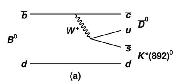
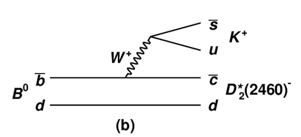
Decay diagrams for the quasi-two-body contributions to $ B ^0 \rightarrow D K ^+ \pi ^- $ from (a) $ B ^0 \rightarrow D K ^* (892)^0$ and (b) $ B ^0 \rightarrow D^{*}_{2}(2460)^{-} K ^+ $ decays.

Results of the fit to the $ B $ candidate invariant mass distribution with (a) linear and (b) logarithmic $y$-axis scales. The components are as described in the legend.

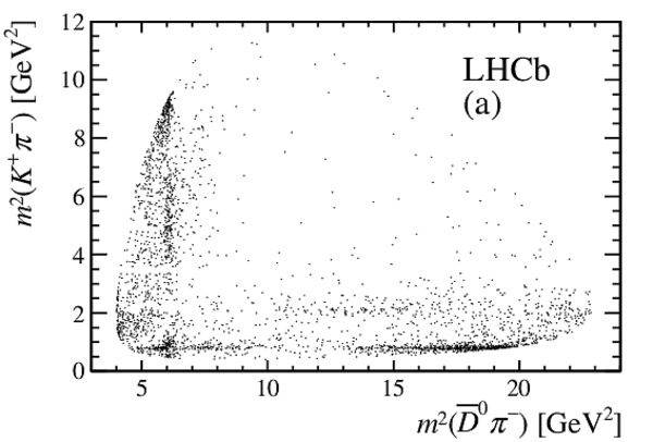
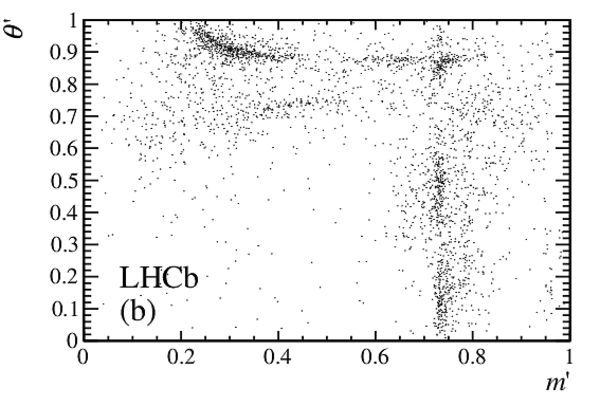
Distribution of $ B ^0 \rightarrow \overline{ D }{} {}^0 K ^+ \pi ^- $ candidates in the signal region over (a) the Dalitz plot and (b) the square Dalitz plot. The definition of the square Dalitz plot is given in Sec. ???.

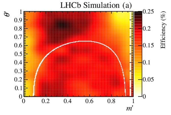
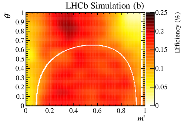
Efficiency variation as a function of SDP position for candidates triggered by (a) signal decay products and (b) by the rest of the event. The vertical white stripe is due to the $ D ^*$ veto and the curved white band is due to the $\overline{ D }{} {}^0$ veto.

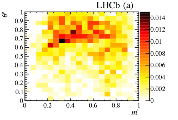
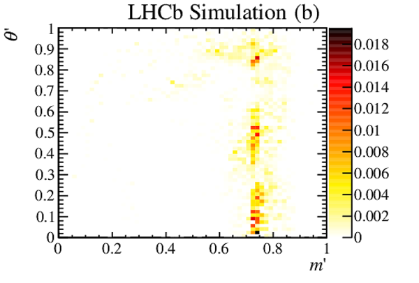
SDP distributions of the background contributions from (a) combinatorial background and (b) $ B ^0 \rightarrow \overline{ D }{} {}^{(*)0} \pi ^+ \pi ^- $ decays.

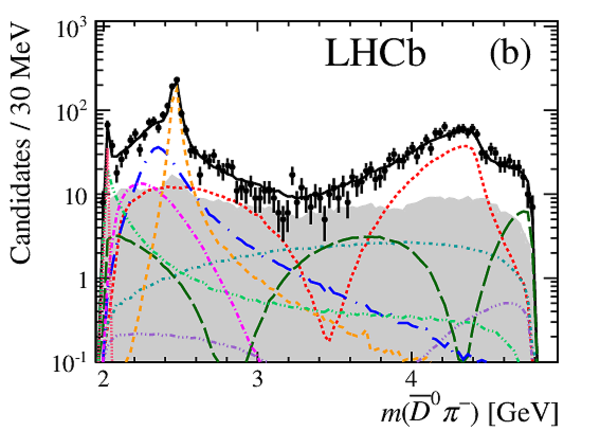
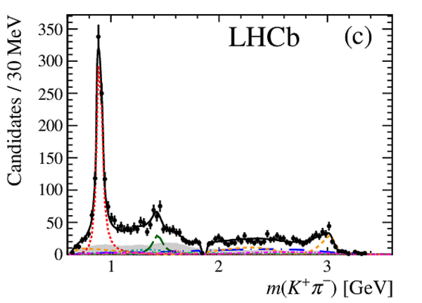
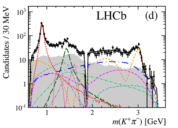
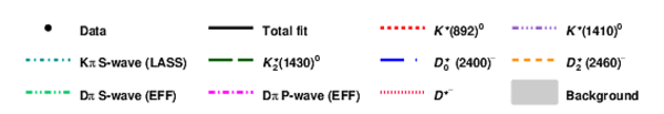
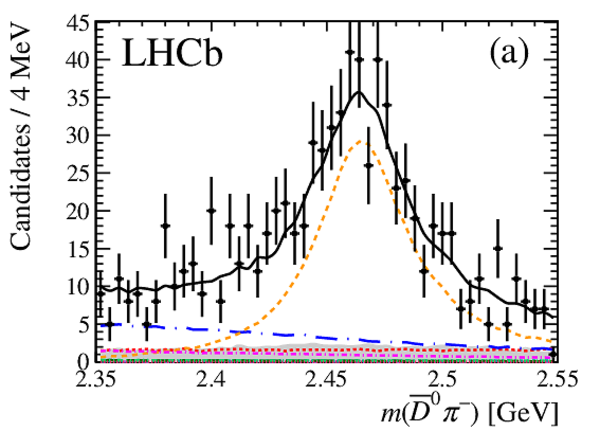
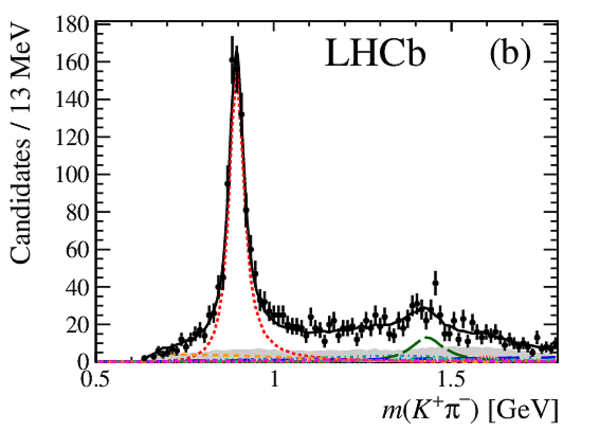
Projections of the data and amplitude fit results onto (a) $m(\overline{ D }{} {}^0 \pi ^- )$, (c) $m( K ^+ \pi ^- )$ and (e) $m(\overline{ D }{} {}^0 K ^+ )$, with the same projections shown in (b), (d) and (f) with a logarithmic $y$-axis scale. Components are described in the legend.

Projections of the data and amplitude fit results onto (a) $m(\overline{ D }{} {}^0 \pi ^- )$ in the $D^*_2(2460)^-$ region and (b) the low $m( K ^+ \pi ^- )$ region. Components are as shown in Fig. ???.

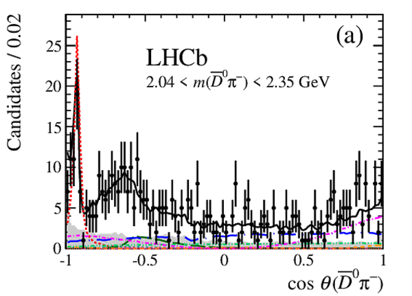
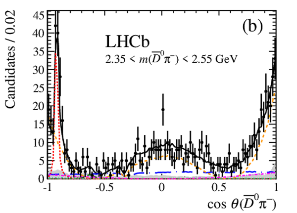
Projections of the data and amplitude fit results onto $\cos \theta(\overline{ D }{} {}^0 \pi ^- )$ in the mass ranges (a) $2.04 < m(\overline{ D }{} {}^0 \pi ^- ) < 2.35 \mathrm{ Ge V} $ and (b) $2.35 < m(\overline{ D }{} {}^0 \pi ^- ) < 2.55 \mathrm{ Ge V} $. Components are as shown in Fig. ???.

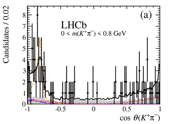
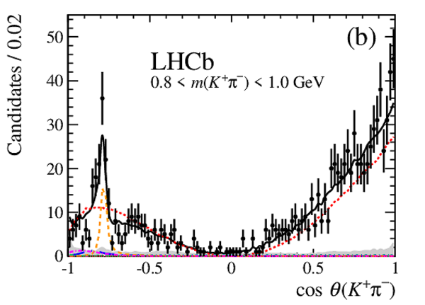
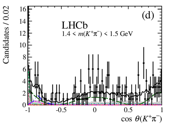
Projections of the data and amplitude fit results onto $\cos \theta( K ^+ \pi ^- )$ in the mass ranges (a) $m( K ^+ \pi ^- ) < 0.8 \mathrm{ Ge V} $, (b) $0.8 < m( K ^+ \pi ^- ) < 1.0 \mathrm{ Ge V} $, (c) $1.0 < m( K ^+ \pi ^- ) < 1.3 \mathrm{ Ge V} $ and (d) $1.4 < m( K ^+ \pi ^- ) < 1.5 \mathrm{ Ge V} $. Components are as shown in Fig. ???.

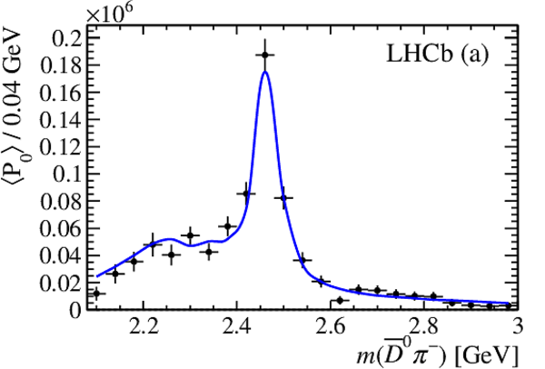
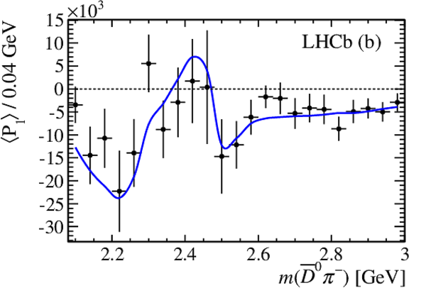
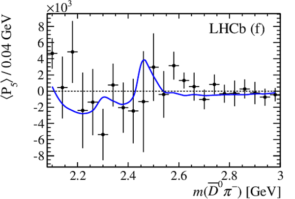
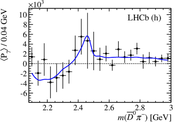
Background-subtracted and efficiency-corrected Legendre moments up to order 7 calculated as a function of $m(\overline{ D }{} {}^0 \pi ^- )$ for data (black data points) and the fit result (solid blue curve).

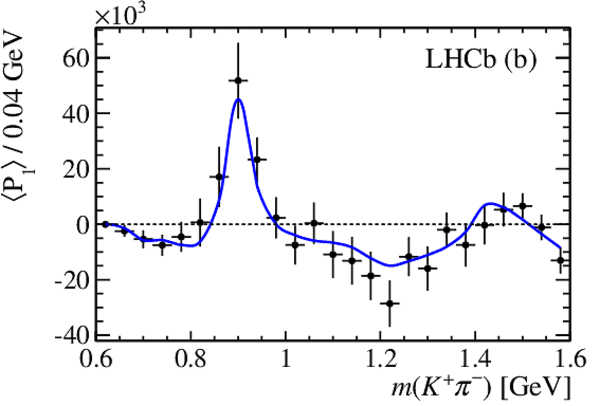
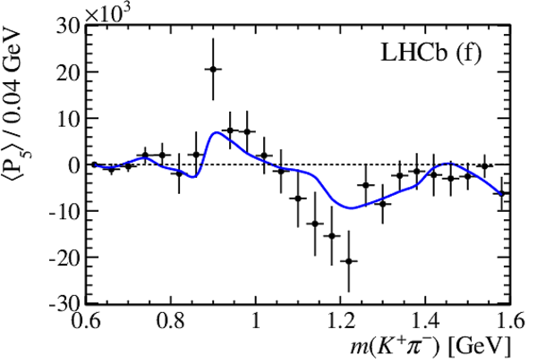
Background-subtracted and efficiency-corrected Legendre moments up to order 7 calculated as a function of $m( K ^+ \pi ^- )$ for data (black data points) and the fit result (solid blue curve).

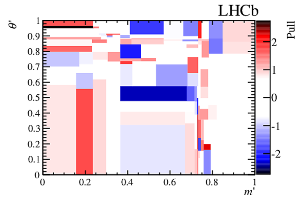
Differences between the data SDP distribution and the fit model across the SDP, in terms of the per-bin pull.

Animated gif made out of all figures.

Yields from the fit to the $\overline{ D }{} {}^0 K ^+ \pi ^- $ data sample. The full mass range is $5100$--$5900\mathrm{ Me V} $ and the signal region is $5248.55$--$5309.05\mathrm{ Me V} $.

Signal contributions to the fit model, where parameters and uncertainties are taken from Ref. \cite{PDG2014}. The models are described in Sec. ???.

Masses and widths $(\mathrm{Me V} )$ determined in the fit to data, with statistical uncertainties only.

Complex coefficients and fit fractions determined from the Dalitz plot fit. Uncertainties are statistical only. Note that the fit fractions, magnitudes and phases are derived quantities.

Experimental systematic uncertainties on the fit fractions (%) and masses and widths $(\mathrm{Me V} )$. Uncertainties given on the central values are statistical only.

Model uncertainties on the fit fractions (%) and masses and widths $(\mathrm{Me V} )$. Uncertainties given on the central values are statistical only.

Results for the complex amplitudes and their uncertainties presented (top) in terms of real and imaginary parts and (bottom) in terms and magnitudes and phases. The three quoted errors are statistical, experimental systematic and model uncertainties, respectively.

Results for the fit fractions and their uncertainties (%). The three quoted errors are statistical, experimental systematic and model uncertainties, respectively. Upper limits are given at 90 % (95 %) confidence level.

Results for the product branching fractions. The four quoted errors are statistical, experimental systematic, model and PDG uncertainties, respectively. Upper limits are given at 90 % (95 %) confidence level.

Results for the branching fractions. The four quoted errors are statistical, experimental systematic, model and PDG uncertainties, respectively. Upper limits are given at 90 % (95 %) confidence level.

Statistical correlations between the real ($x$) and imaginary ($y$) parts of the complex coefficients that are free parameters of the fit. Correlations with the masses ($m$) and widths ($\Gamma$) that are determined from the fit are also included. The correlations are determined from the same sample of simulated pseudoexperiments used to evaluate systematic uncertainties. The labels correspond to: (0) $ K ^* (892)^{0}$, (1) $ K ^* (1410)^{0}$, (2) $ K ^*_{0}(1430)^{0}$, (3) LASS nonresonant, (4) $ K ^*_{2}(1430)^{0}$, (5) $D^{*}_{0}(2400)^{-}$, (6) $D^{*}_{2}(2460)^{-}$, (7) $D\pi$ S-wave (dabba), (8) $D\pi$ P-wave (EFF).

Statistical correlations between the magnitudes ($a$) and phases ($\Delta$) of the complex coefficients that are free parameters of the fit. Correlations with the masses ($m$) and widths ($\Gamma$) that are determined from the fit are also included. The correlations are determined from the same sample of simulated pseudoexperiments used to evaluate systematic uncertainties. The labels correspond to: (0) $ K ^* (892)^{0}$, (1) $ K ^* (1410)^{0}$, (2) $ K ^*_{0}(1430)^{0}$, (3) LASS nonresonant, (4) $ K ^*_{2}(1430)^{0}$, (5) $D^{*}_{0}(2400)^{-}$, (6) $D^{*}_{2}(2460)^{-}$, (7) $D\pi$ S-wave (dabba), (8) $D\pi$ P-wave (EFF).

Interference fit fractions (%) from the nominal DP fit. The amplitudes are all pairwise products involving: ($A_{0}$) $ K ^* (892)^{0}$, ($A_{1}$) $ K ^* (1410)^{0}$, ($A_{2}$) $ K ^*_{0}(1430)^{0}$, ($A_{3}$) LASS nonresonant, ($A_{4}$) $ K ^*_{2}(1430)^{0}$, ($A_{5}$) $D^{*}_{0}(2400)^{-}$, ($A_{6}$) $D^{*}_{2}(2460)^{-}$, ($A_{7}$) $D\pi$ S-wave (dabba), ($A_{8}$) $D\pi$ P-wave (EFF). The diagonal elements are the same as the conventional fit fractions.

Statistical uncertainties on the interference fit fractions (%). The amplitudes are all pairwise products involving: ($A_{0}$) $ K ^* (892)^{0}$, ($A_{1}$) $ K ^* (1410)^{0}$, ($A_{2}$) $ K ^*_{0}(1430)^{0}$, ($A_{3}$) LASS nonresonant, ($A_{4}$) $ K ^*_{2}(1430)^{0}$, ($A_{5}$) $D^{*}_{0}(2400)^{-}$, ($A_{6}$) $D^{*}_{2}(2460)^{-}$, ($A_{7}$) $D\pi$ S-wave (dabba), ($A_{8}$) $D\pi$ P-wave (EFF). The diagonal elements are the same as the conventional fit fractions.

Experimental systematic uncertainties on the interference fit fractions (%). The amplitudes are all pairwise products involving: ($A_{0}$) $ K ^* (892)^{0}$, ($A_{1}$) $ K ^* (1410)^{0}$, ($A_{2}$) $ K ^*_{0}(1430)^{0}$, ($A_{3}$) LASS nonresonant, ($A_{4}$) $ K ^*_{2}(1430)^{0}$, ($A_{5}$) $D^{*}_{0}(2400)^{-}$, ($A_{6}$) $D^{*}_{2}(2460)^{-}$, ($A_{7}$) $D\pi$ S-wave (dabba), ($A_{8}$) $D\pi$ P-wave (EFF). The diagonal elements are the same as the conventional fit fractions.

Model uncertainties on the interference fit fractions (%). The amplitudes are all pairwise products involving: ($A_{0}$) $ K ^* (892)^{0}$, ($A_{1}$) $ K ^* (1410)^{0}$, ($A_{2}$) $ K ^*_{0}(1430)^{0}$, ($A_{3}$) LASS nonresonant, ($A_{4}$) $ K ^*_{2}(1430)^{0}$, ($A_{5}$) $D^{*}_{0}(2400)^{-}$, ($A_{6}$) $D^{*}_{2}(2460)^{-}$, ($A_{7}$) $D\pi$ S-wave (dabba), ($A_{8}$) $D\pi$ P-wave (EFF). The diagonal elements are the same as the conventional fit fractions.