Studies of the resonance structure in $D^0\to K^0_S K^{\pm}\pi^{\mp}$ decays
[to restricted-access page]Information
LHCb-PAPER-2015-026
CERN-PH-EP-2015-238
arXiv:1509.06628 [PDF]
(Submitted on 22 Sep 2015)
Phys. Rev. D93 (2016) 052018
Inspire 1394391
Tools
Abstract
Amplitude models are applied to studies of resonance structure in $D^0\to K^0_S K^- \pi^+$ and $D^0\to K^0_S K^+ \pi^-$ decays using $pp$ collision data corresponding to an integrated luminosity of $3.0 \mathrm{fb}^{-1}$ collected by the LHCb experiment. Relative magnitude and phase information is determined, and coherence factors and related observables are computed for both the whole phase space and a restricted region of $100 \mathrm{MeV/}c^2$ around the $K^{*}(892)^{\pm}$ resonance. Two formulations for the $K\pi$ $S$-wave are used, both of which give a good description of the data. The ratio of branching fractions $\mathcal{B}(D^0\to K^0_S K^+ \pi^-)/\mathcal{B}(D^0\to K^0_S K^- \pi^+)$ is measured to be $0.655\pm0.004 (\textrm{stat})\pm0.006 (\textrm{syst})$ over the full phase space and $0.370\pm0.003 (\textrm{stat})\pm0.012 (\textrm{syst})$ in the restricted region. A search for $CP$ violation is performed using the amplitude models and no significant effect is found. Predictions from $SU(3)$ flavor symmetry for $K^{*}(892)K$ amplitudes of different charges are compared with the amplitude model results.
Figures and captions
|
SCS classes of diagrams contributing to the decays $ D ^0 \rightarrow K ^0_{\rm\scriptscriptstyle S} K ^\pm \pi ^\mp $ . The color-favored (tree) diagrams (a) contribute to the $ K ^{*{\pm}}_{0,1,2} \rightarrow K ^0_{\rm\scriptscriptstyle S} \pi ^\pm $ and $ ( a ^{{}}_{0,2} ,\rho )^{\pm} \rightarrow K ^0_{\rm\scriptscriptstyle S} K ^\pm $ channels, while the color-suppressed exchange diagrams (b) contribute to the $ ( a ^{{}}_{0,2} ,\rho )^{\pm} \rightarrow K ^0_{\rm\scriptscriptstyle S} K ^\pm $ , $ K ^{*{0}}_{0,1,2} \rightarrow K ^+ \pi ^- $ and $\overline{ K }{} ^{*{0}}_{0,1,2} \rightarrow K ^- \pi ^+ $ channels. Second-order loop (penguin) diagrams (c) contribute to the $ ( a ^{{}}_{0,2} ,\rho )^{\pm} \rightarrow K ^0_{\rm\scriptscriptstyle S} K ^\pm $ and $ K ^{*{\pm}}_{0,1,2} \rightarrow K ^0_{\rm\scriptscriptstyle S} \pi ^\pm $ channels, and, finally, OZI-suppressed penguin annihilation diagrams (d) contribute to all decay channels. |
[Failure to get the plot] | |
|
Mass (left) and $\Delta m$ (right) distributions for the $ D ^0 \rightarrow K ^0_{\rm\scriptscriptstyle S} K ^- \pi ^+ $ (top) and $ D ^0 \rightarrow K ^0_{\rm\scriptscriptstyle S} K ^+ \pi ^- $ (bottom) samples with fit results superimposed. The long-dashed (blue) curve represents the $ D ^{*}({{2010}})^{{+}}$ signal, the dash-dotted (green) curve represents the contribution of real $ D ^0$ mesons combined with incorrect $\pi ^{+}_{\text{slow}}$ and the dotted (red) curve represents the combined combinatorial and $ D ^0 \rightarrow K ^0_{\rm\scriptscriptstyle S} \pi ^+ \pi ^- \pi ^0 $ background contribution. The vertical solid lines show the signal region boundaries, and the vertical dotted lines show the sideband region boundaries. |
Fig_2.pdf [1 KiB] HiDef png [1 KiB] Thumbnail [0 KiB] *.C file tex code |

|
|
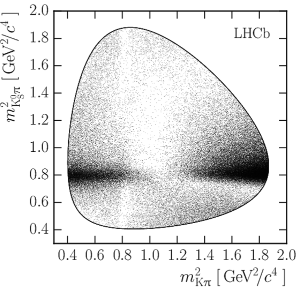
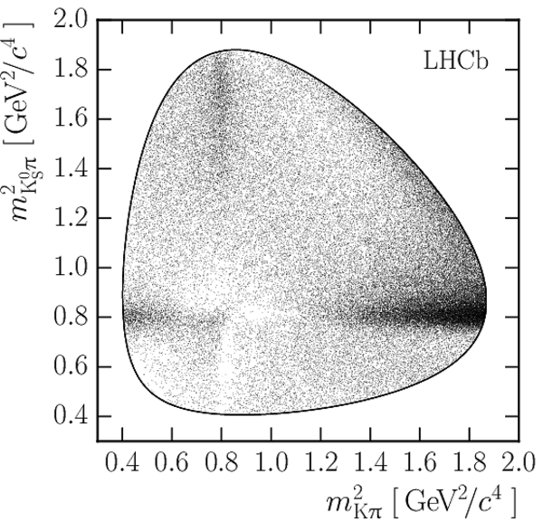
Dalitz plots of the $ D ^0 \rightarrow K ^0_{\rm\scriptscriptstyle S} K ^- \pi ^+ $ (left) and $ D ^0 \rightarrow K ^0_{\rm\scriptscriptstyle S} K ^+ \pi ^- $ (right) candidates in the two-dimensional signal region. |
rd_tos[..].pdf [472 KiB] HiDef png [1 MiB] Thumbnail [313 KiB] *.C file |
|
|
rd_tos[..].pdf [527 KiB] HiDef png [1 MiB] Thumbnail [339 KiB] *.C file |
|
|
|
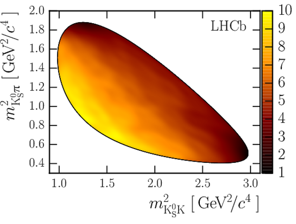
Efficiency function used in the isobar model fits, corresponding to the average efficiency over the full dataset. The coordinates $ m^{2}_{ K ^0_{\rm\scriptscriptstyle S} \pi }$ and $ m^{2}_{ K ^0_{\rm\scriptscriptstyle S} K }$ are used to highlight the approximate symmetry of the efficiency function. The $z$ units are arbitrary. |
efficiency.pdf [178 KiB] HiDef png [1 MiB] Thumbnail [341 KiB] *.C file |
|
|
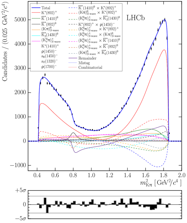
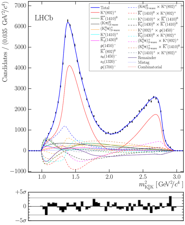
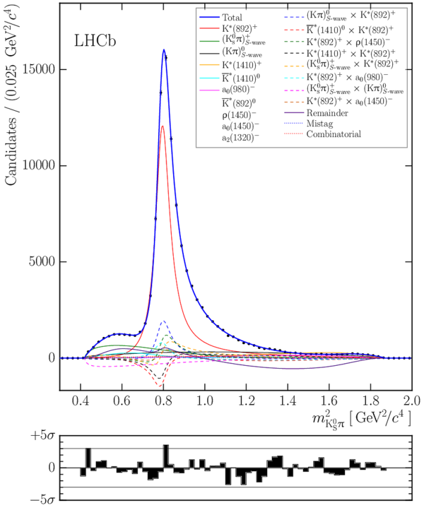
Distributions of $ m^{2}_{ K \pi }$ (upper left), $ m^{2}_{ K ^0_{\rm\scriptscriptstyle S} \pi }$ (upper right) and $ m^{2}_{ K ^0_{\rm\scriptscriptstyle S} K }$ (lower left) in the $ D ^0 \rightarrow K ^0_{\rm\scriptscriptstyle S} K ^- \pi ^+ $ mode with fit curves from the best \texttt{GLASS} model. The solid (blue) curve shows the full PDF $P_{ K ^0_{\rm\scriptscriptstyle S} K ^- \pi ^+ }( m^{2}_{ K ^0_{\rm\scriptscriptstyle S} \pi } , m^{2}_{ K \pi } )$, while the other curves show the components with the largest integrated fractions. |
[Failure to get the plot] | [Failure to get the plot] | [Failure to get the plot] | [Failure to get the plot] |
|
Distributions of $ m^{2}_{ K \pi }$ (upper left), $ m^{2}_{ K ^0_{\rm\scriptscriptstyle S} \pi }$ (upper right) and $ m^{2}_{ K ^0_{\rm\scriptscriptstyle S} K }$ (lower left) in the $ D ^0 \rightarrow K ^0_{\rm\scriptscriptstyle S} K ^- \pi ^+ $ mode with fit curves from the best \texttt{LASS} model. The solid (blue) curve shows the full PDF $P_{ K ^0_{\rm\scriptscriptstyle S} K ^- \pi ^+ }( m^{2}_{ K ^0_{\rm\scriptscriptstyle S} \pi } , m^{2}_{ K \pi } )$, while the other curves show the components with the largest integrated fractions. |
[Failure to get the plot] | [Failure to get the plot] | [Failure to get the plot] | [Failure to get the plot] |
|
Distributions of $ m^{2}_{ K \pi }$ (upper left), $ m^{2}_{ K ^0_{\rm\scriptscriptstyle S} \pi }$ (upper right) and $ m^{2}_{ K ^0_{\rm\scriptscriptstyle S} K }$ (lower left) in the $ D ^0 \rightarrow K ^0_{\rm\scriptscriptstyle S} K ^+ \pi ^- $ mode with fit curves from the best \texttt{GLASS} model. The solid (blue) curve shows the full PDF $P_{ K ^0_{\rm\scriptscriptstyle S} K ^+ \pi ^- }( m^{2}_{ K ^0_{\rm\scriptscriptstyle S} \pi } , m^{2}_{ K \pi } )$, while the other curves show the components with the largest integrated fractions. |
[Failure to get the plot] | [Failure to get the plot] | [Failure to get the plot] | [Failure to get the plot] |
|
Distributions of $ m^{2}_{ K \pi }$ (upper left), $ m^{2}_{ K ^0_{\rm\scriptscriptstyle S} \pi }$ (upper right) and $ m^{2}_{ K ^0_{\rm\scriptscriptstyle S} K }$ (lower left) in the $ D ^0 \rightarrow K ^0_{\rm\scriptscriptstyle S} K ^+ \pi ^- $ mode with fit curves from the best \texttt{LASS} model. The solid (blue) curve shows the full PDF $P_{ K ^0_{\rm\scriptscriptstyle S} K ^+ \pi ^- }( m^{2}_{ K ^0_{\rm\scriptscriptstyle S} \pi } , m^{2}_{ K \pi } )$, while the other curves show the components with the largest integrated fractions. |
[Failure to get the plot] | [Failure to get the plot] | [Failure to get the plot] | [Failure to get the plot] |
|
Decay rate and phase variation across the Dalitz plot. The top row shows $|\mathcal{M} _{ K ^0_{\rm\scriptscriptstyle S} K ^\pm \pi ^\mp }( m^{2}_{ K ^0_{\rm\scriptscriptstyle S} \pi } , m^{2}_{ K \pi } )|^2$ in the best \texttt{GLASS} isobar models, the center row shows the phase behavior of the same models and the bottom row shows the same function subtracted from the phase behavior in the best \texttt{LASS} isobar models. The left column shows the $ D ^0 \rightarrow K ^0_{\rm\scriptscriptstyle S} K ^- \pi ^+ $ mode with $ D ^0 \rightarrow K ^0_{\rm\scriptscriptstyle S} K ^+ \pi ^- $ on the right. The small inhomogeneities that are visible in the bottom row relate to the \texttt{GLASS} and \texttt{LASS} models preferring slightly different values of the $ K ^{*}_{{}}({892})^{{\pm}}$ mass and width. |
[Failure to get the plot] | [Failure to get the plot] | [Failure to get the plot] | [Failure to get the plot] | [Failure to get the plot] | [Failure to get the plot] |
|
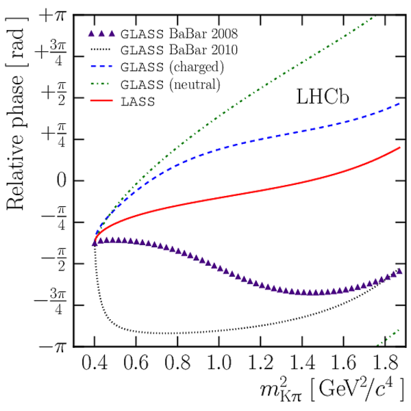
Comparison of the phase behavior of the various $ K \pi $ $S$-wave parameterizations used. The solid (red) curve shows the \texttt{LASS} parameterization, while the dashed (blue) and dash-dotted (green) curves show, respectively, the \texttt{GLASS} functional form fitted to the charged and neutral $S$-wave channels. The final two curves show the \texttt{GLASS} forms fitted to the charged $ K \pi $ $S$-wave in $ D ^0 \rightarrow K ^0_{\rm\scriptscriptstyle S} \pi ^+ \pi ^- $ decays in Ref. \cite{Aubert:2008bd} (triangular markers, purple) and Ref. \cite{delAmoSanchez:2010xz} (dotted curve, black). The latter of these was used in the analysis of $ D ^0 \rightarrow K ^0_{\rm\scriptscriptstyle S} K ^\pm \pi ^\mp $ decays by the CLEO collaboration \cite{Insler:2012pm}. |
lass_g[..].pdf [168 KiB] HiDef png [282 KiB] Thumbnail [227 KiB] *.C file |
|
|
Smooth functions, $c_{ K ^0_{\rm\scriptscriptstyle S} K ^\pm \pi ^\mp }( m^{2}_{ K ^0_{\rm\scriptscriptstyle S} K } , m^{2}_{ K ^0_{\rm\scriptscriptstyle S} \pi } )$, used to describe the combinatorial background component in the $ D ^0 \rightarrow K ^0_{\rm\scriptscriptstyle S} K ^- \pi ^+ $ (left) and $ D ^0 \rightarrow K ^0_{\rm\scriptscriptstyle S} K ^+ \pi ^- $ (right) amplitude model fits. |
[Failure to get the plot] | [Failure to get the plot] |
|
Two-dimensional quality-of-fit distributions illustrating the dynamic binning scheme used to evaluate $\chi^2$ . The variable shown is $\frac{d_i - p_i}{\sqrt{p_i}}$ where $d_i$ and $p_i$ are the number of events and the fitted value, respectively, in bin $i$. The $ D ^0 \rightarrow K ^0_{\rm\scriptscriptstyle S} K ^- \pi ^+ $ ( $ D ^0 \rightarrow K ^0_{\rm\scriptscriptstyle S} K ^+ \pi ^- $ ) mode is shown in the left (right) column, and the \texttt{GLASS} (\texttt{LASS} ) isobar models are shown in the top (bottom) row. |
[Failure to get the plot] | [Failure to get the plot] | [Failure to get the plot] | [Failure to get the plot] |
|
Animated gif made out of all figures. |
PAPER-2015-026.gif Thumbnail |

|
Tables and captions
|
Signal yields and estimated background rates in the two-dimensional signal region. The larger mistag rate in the $ D ^0 \rightarrow K ^0_{\rm\scriptscriptstyle S} K ^+ \pi ^- $ mode is due to the different branching fractions for the two modes. Only statistical uncertainties are quoted. |
Table_1.pdf [52 KiB] HiDef png [41 KiB] Thumbnail [18 KiB] tex code |

|
|
Blatt-Weisskopf centrifugal barrier penetration factors, $B_J(q, q_0, d)$ \cite{BlattWeisskopf}. |
Table_2.pdf [47 KiB] HiDef png [98 KiB] Thumbnail [36 KiB] tex code |

|
|
Angular distribution factors, $\Omega_J(p_{ D ^0 } + p_{ C }, p_{ B } - p_{ A })$. These are expressed in terms of the tensors $T^{\mu\nu} = -g^{\mu\nu} + \frac{p^\mu_{ A B }p^\nu_{ A B }}{ m_{ R }^{2} }$ and $T^{\mu\nu\alpha\beta} = \frac{1}{2}(T^{\mu\alpha}T^{\nu\beta} + T^{\mu\beta}T^{\nu\alpha}) - \frac{1}{3}T^{\mu\nu}T^{\alpha\beta}$. |
Table_3.pdf [49 KiB] HiDef png [38 KiB] Thumbnail [17 KiB] tex code |

|
|
Particle ordering conventions used in this analysis. |
Table_4.pdf [48 KiB] HiDef png [35 KiB] Thumbnail [16 KiB] tex code |

|
|
Isobar model fit results for the $ D ^0 \rightarrow K ^0_{\rm\scriptscriptstyle S} K ^- \pi ^+ $ mode. The first uncertainties are statistical and the second systematic. |
Table_5.pdf [71 KiB] Thumbnail [36 KiB] tex code |

|
|
Isobar model fit results for the $ D ^0 \rightarrow K ^0_{\rm\scriptscriptstyle S} K ^+ \pi ^- $ mode. The first uncertainties are statistical and the second systematic. |
Table_6.pdf [71 KiB] Thumbnail [34 KiB] tex code |

|
|
Modulus and phase of the relative amplitudes between resonances that appear in both the $ D ^0 \rightarrow K ^0_{\rm\scriptscriptstyle S} K ^- \pi ^+ $ and $ D ^0 \rightarrow K ^0_{\rm\scriptscriptstyle S} K ^+ \pi ^- $ modes. Relative phases are calculated using the value of $\delta_{ K ^0_{\rm\scriptscriptstyle S} K \pi }$ measured in $\psi (3770)$ decays \cite{Insler:2012pm}, and the uncertainty on this value is included in the statistical uncertainty. The first uncertainties are statistical and the second systematic. |
Table_7.pdf [86 KiB] HiDef png [190 KiB] Thumbnail [97 KiB] tex code |

|
|
Values of $\chi^2/\mathrm{bin}$ indicating the fit quality obtained using both $ K \pi $ $S$-wave parameterizations in the two decay modes. The binning scheme for the $ D ^0 \rightarrow K ^0_{\rm\scriptscriptstyle S} K ^- \pi ^+ $ ( $ D ^0 \rightarrow K ^0_{\rm\scriptscriptstyle S} K ^+ \pi ^- $ ) mode contains 2191 (2573) bins. |
Table_8.pdf [57 KiB] HiDef png [53 KiB] Thumbnail [21 KiB] tex code |

|
|
Coherence factor observables to which the isobar models are sensitive. The third column summarizes the CLEO results measured in quantum-correlated decays \cite{Insler:2012pm}, where the uncertainty on $\delta_{ K ^0_{\rm\scriptscriptstyle S} K \pi } - \delta_{ K ^* K }$ is calculated assuming maximal correlation between $\delta_{ K ^0_{\rm\scriptscriptstyle S} K \pi }$ and $\delta_{ K ^* K }$. |
Table_9.pdf [66 KiB] HiDef png [39 KiB] Thumbnail [17 KiB] tex code |

|
|
$\mathrm{SU}(3)$ flavor symmetry predictions \cite{Bhattacharya:2012fz} and results. The uncertainties on phase difference predictions are calculated from the quoted magnitude and phase uncertainties. Note that some theoretical predictions depend on the $\eta $ -- $\eta ^{\prime}$ mixing angle $\theta_{\eta -\eta ^{\prime} }$ and are quoted for two different values. The bottom entry in the table relies on the CLEO measurement \cite{Insler:2012pm} of the coherence factor phase $\delta_{ K ^0_{\rm\scriptscriptstyle S} K \pi }$, and the uncertainty on this phase is included in the statistical uncertainty, while the other entries are calculated directly from the isobar models and relative branching ratio. Where two uncertainties are quoted the first is statistical and the second systematic. |
Table_10.pdf [77 KiB] HiDef png [90 KiB] Thumbnail [40 KiB] tex code |

|
|
$ C P$ violation fit results. Results are only shown for those resonances that appear in both the \texttt{GLASS} and \texttt{LASS} models. The first uncertainties are statistical and the second systematic; the only systematic uncertainty is that due to the choice of isobar model. |
Table_11.pdf [72 KiB] HiDef png [62 KiB] Thumbnail [22 KiB] tex code |

|
|
Nominal values for isobar model parameters that are fixed in the model fits, or used in constraint terms. These values are taken from Refs. \cite{PDG2014,Abele:1998qd,Bargiotti:2003ev,Dunwoodie} as described in Sect. ???. |
Table_12.pdf [72 KiB] HiDef png [304 KiB] Thumbnail [145 KiB] tex code |

|
|
Interference fractions for the $ D ^0 \rightarrow K ^0_{\rm\scriptscriptstyle S} K ^- \pi ^+ $ mode. The first uncertainties are statistical and the second systematic. Only the 25 largest terms are shown. |
Table_13.pdf [62 KiB] HiDef png [338 KiB] Thumbnail [157 KiB] tex code |

|
|
Interference fractions for the $ D ^0 \rightarrow K ^0_{\rm\scriptscriptstyle S} K ^+ \pi ^- $ mode. The first uncertainties are statistical and the second systematic. Only the 25 largest terms are shown. |
Table_14.pdf [62 KiB] HiDef png [334 KiB] Thumbnail [155 KiB] tex code |

|
|
Matrices $\mathbf{U}$ relating the fit coordinates $\mathbf{b'}$ to the \texttt{LASS} form factor coordinates $\mathbf{b}=\mathbf{Ub'}$ defined in Sect. ???. |
Table_15.pdf [62 KiB] HiDef png [43 KiB] Thumbnail [20 KiB] tex code |

|
|
Additional fit parameters for \texttt{GLASS} models. This table does not include parameters that are fixed to their nominal values. The first uncertainties are statistical and the second systematic. |
Table_16.pdf [63 KiB] HiDef png [171 KiB] Thumbnail [87 KiB] tex code |

|
|
Additional fit parameters for \texttt{LASS} models. This table does not include parameters that are fixed to their nominal values. The first uncertainties are statistical and the second systematic. |
Table_17.pdf [63 KiB] HiDef png [161 KiB] Thumbnail [81 KiB] tex code |

|
|
Change in $ -2\log\mathcal{L}$ value when removing a $\rho $ resonance from one of the models. |
Table_18.pdf [61 KiB] HiDef png [61 KiB] Thumbnail [28 KiB] tex code |

|
|
Listing of abbreviations required to typeset the systematic uncertainty tables. |
Table_19.pdf [77 KiB] HiDef png [268 KiB] Thumbnail [115 KiB] tex code |

|
|
Systematic uncertainties for complex amplitudes and fit fractions in the $ D ^0 \rightarrow K ^0_{\rm\scriptscriptstyle S} K ^- \pi ^+ $ model using the \texttt{GLASS} parameterization. The headings are defined in Table ???. |
Table_20.pdf [74 KiB] HiDef png [188 KiB] Thumbnail [70 KiB] tex code |

|
|
Systematic uncertainties for complex amplitudes and fit fractions in the $ D ^0 \rightarrow K ^0_{\rm\scriptscriptstyle S} K ^- \pi ^+ $ model using the \texttt{LASS} parameterization. The headings are defined in Table ???. |
Table_21.pdf [74 KiB] HiDef png [166 KiB] Thumbnail [68 KiB] tex code |

|
|
Systematic uncertainties for complex amplitudes and fit fractions in the $ D ^0 \rightarrow K ^0_{\rm\scriptscriptstyle S} K ^+ \pi ^- $ model using the \texttt{GLASS} parameterization. The headings are defined in Table ???. |
Table_22.pdf [74 KiB] HiDef png [185 KiB] Thumbnail [70 KiB] tex code |

|
|
Systematic uncertainties for complex amplitudes and fit fractions in the $ D ^0 \rightarrow K ^0_{\rm\scriptscriptstyle S} K ^+ \pi ^- $ model using the \texttt{LASS} parameterization. The headings are defined in Table ???. |
Table_23.pdf [74 KiB] HiDef png [126 KiB] Thumbnail [59 KiB] tex code |

|
|
Systematic uncertainties for shared parameters, coherence and relative branching ratio observables in the \texttt{GLASS} models. The systematic uncertainty on the $ K ^{*}_{{}}({892})^{{\pm}}$ width due to neglecting resolution effects in the nominal models is $0.5 {\mathrm{ Me V /}c^2} $. |
Table_24.pdf [78 KiB] HiDef png [132 KiB] Thumbnail [47 KiB] tex code |

|
|
Systematic uncertainties for shared parameters, coherence and relative branching ratio observables in the \texttt{LASS} models. The systematic uncertainty on the $ K ^{*}_{{}}({892})^{{\pm}}$ width due to neglecting resolution effects in the nominal models is $0.6 {\mathrm{ Me V /}c^2} $. |
Table_25.pdf [79 KiB] HiDef png [117 KiB] Thumbnail [43 KiB] tex code |

|
|
Full $ C P$ violation fit results as described in Sect. ???. The only uncertainties included are statistical. |
Table_26.pdf [71 KiB] HiDef png [75 KiB] Thumbnail [23 KiB] tex code |

|
|
Lookup table filenames. |
Table_27.pdf [60 KiB] HiDef png [42 KiB] Thumbnail [19 KiB] tex code |

|
Supplementary Material [file]


![HiDef png [1 KiB]](Directory_LHCb-PAPER-2015-026/hidef_Fig_2.png)
![HiDef png [1 MiB]](Directory_LHCb-PAPER-2015-026/hidef_rd_tos_fav_sig_scatter_mpl.png)
![HiDef png [1 MiB]](Directory_LHCb-PAPER-2015-026/hidef_rd_tos_sup_sig_scatter_mpl.png)
![HiDef png [1 MiB]](Directory_LHCb-PAPER-2015-026/hidef_efficiency.png)
![HiDef png [282 KiB]](Directory_LHCb-PAPER-2015-026/hidef_lass_glass_comparison.png)
![HiDef png [41 KiB]](Directory_LHCb-PAPER-2015-026/hidef_Table_1.png)
![HiDef png [98 KiB]](Directory_LHCb-PAPER-2015-026/hidef_Table_2.png)
![HiDef png [38 KiB]](Directory_LHCb-PAPER-2015-026/hidef_Table_3.png)
![HiDef png [35 KiB]](Directory_LHCb-PAPER-2015-026/hidef_Table_4.png)
![HiDef png [190 KiB]](Directory_LHCb-PAPER-2015-026/hidef_Table_7.png)
![HiDef png [53 KiB]](Directory_LHCb-PAPER-2015-026/hidef_Table_8.png)
![HiDef png [39 KiB]](Directory_LHCb-PAPER-2015-026/hidef_Table_9.png)
![HiDef png [90 KiB]](Directory_LHCb-PAPER-2015-026/hidef_Table_10.png)
![HiDef png [62 KiB]](Directory_LHCb-PAPER-2015-026/hidef_Table_11.png)
![HiDef png [304 KiB]](Directory_LHCb-PAPER-2015-026/hidef_Table_12.png)
![HiDef png [338 KiB]](Directory_LHCb-PAPER-2015-026/hidef_Table_13.png)
![HiDef png [334 KiB]](Directory_LHCb-PAPER-2015-026/hidef_Table_14.png)
![HiDef png [43 KiB]](Directory_LHCb-PAPER-2015-026/hidef_Table_15.png)
![HiDef png [171 KiB]](Directory_LHCb-PAPER-2015-026/hidef_Table_16.png)
![HiDef png [161 KiB]](Directory_LHCb-PAPER-2015-026/hidef_Table_17.png)
![HiDef png [61 KiB]](Directory_LHCb-PAPER-2015-026/hidef_Table_18.png)
![HiDef png [268 KiB]](Directory_LHCb-PAPER-2015-026/hidef_Table_19.png)
![HiDef png [188 KiB]](Directory_LHCb-PAPER-2015-026/hidef_Table_20.png)
![HiDef png [166 KiB]](Directory_LHCb-PAPER-2015-026/hidef_Table_21.png)
![HiDef png [185 KiB]](Directory_LHCb-PAPER-2015-026/hidef_Table_22.png)
![HiDef png [126 KiB]](Directory_LHCb-PAPER-2015-026/hidef_Table_23.png)
![HiDef png [132 KiB]](Directory_LHCb-PAPER-2015-026/hidef_Table_24.png)
![HiDef png [117 KiB]](Directory_LHCb-PAPER-2015-026/hidef_Table_25.png)
![HiDef png [75 KiB]](Directory_LHCb-PAPER-2015-026/hidef_Table_26.png)
![HiDef png [42 KiB]](Directory_LHCb-PAPER-2015-026/hidef_Table_27.png)
![HiDef png [523 KiB]](Directory_LHCb-PAPER-2015-026/supplementary/hidef_Fig1-S.png)
![HiDef png [502 KiB]](Directory_LHCb-PAPER-2015-026/supplementary/hidef_Fig10-S.png)
![HiDef png [467 KiB]](Directory_LHCb-PAPER-2015-026/supplementary/hidef_Fig11-S.png)
![HiDef png [455 KiB]](Directory_LHCb-PAPER-2015-026/supplementary/hidef_Fig12-S.png)
![HiDef png [455 KiB]](Directory_LHCb-PAPER-2015-026/supplementary/hidef_Fig2-S.png)
![HiDef png [536 KiB]](Directory_LHCb-PAPER-2015-026/supplementary/hidef_Fig3-S.png)
![HiDef png [509 KiB]](Directory_LHCb-PAPER-2015-026/supplementary/hidef_Fig4-S.png)
![HiDef png [432 KiB]](Directory_LHCb-PAPER-2015-026/supplementary/hidef_Fig5-S.png)
![HiDef png [505 KiB]](Directory_LHCb-PAPER-2015-026/supplementary/hidef_Fig6-S.png)
![HiDef png [541 KiB]](Directory_LHCb-PAPER-2015-026/supplementary/hidef_Fig7-S.png)
![HiDef png [490 KiB]](Directory_LHCb-PAPER-2015-026/supplementary/hidef_Fig8-S.png)
![HiDef png [502 KiB]](Directory_LHCb-PAPER-2015-026/supplementary/hidef_Fig9-S.png)
Created on 27 April 2024.