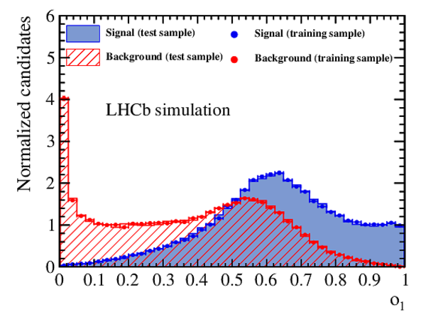
(left) Distribution of the NN1 output, $o_1$, of signal (blue) and background (red) tracks. (right) Distribution of the NN2 output, $o_2$, of initially produced $ B ^0_ s $ (blue) and $\overline{ B }{} {}^0_ s $ (red) mesons. Both distributions are obtained with simulated events. The markers represent the distributions obtained from the training samples; the solid histograms are the distributions obtained from the test samples. The good agreement between the distributions of the test and training samples shows that there is no overtraining of the classifiers.

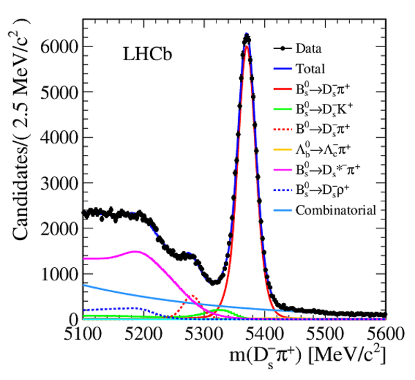
Mass distribution of $ B ^0_ s \rightarrow D ^-_ s \pi ^+ $ candidates with fit projections overlaid. Data points (black markers) correspond to the $ B ^0_ s $ candidates selected in the 3 $ fb^{-1}$ data sample. The total fit function and its components are overlaid with solid and dashed lines (see legend).

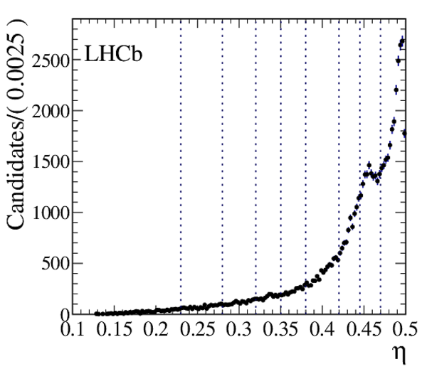
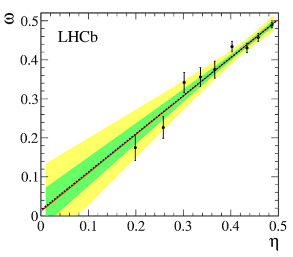
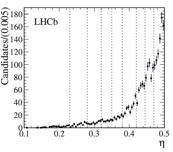
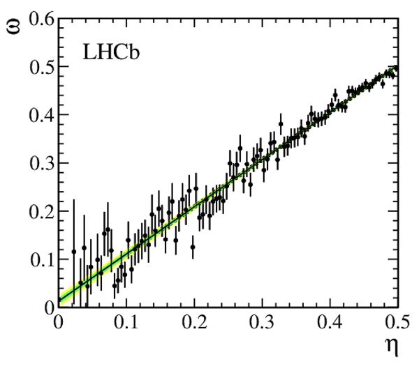
(left) Background-subtracted $\eta$ distribution of $ B ^0_ s \rightarrow D ^-_ s \pi ^+ $ candidates in data; the vertical dotted lines show the binning used in the second method of the calibration. (right) Measured average mistag fraction $\omega$ in bins of mistag probability $\eta$ (black points), with the result of a linear fit superimposed (solid red line) and compared to the calibration obtained from the unbinned fit (dashed black line). The linear fit has $\chi^2/\mathrm{ndf} =1.3$. The shaded areas correspond to the 68% and 95% confidence level regions of the unbinned fit.

Distribution of the mass difference, $Q$, of selected $ B ^+ K ^- $ candidates, summing over four $ B ^+$ decay modes (black points), and the function fitted to these data (solid blue line). From left to right, the three peaks are identified as being $ B _{ s 1}(5830)^0\rightarrow B ^{*+} K ^- $, $ B _{ s 2}^{*}(5840)^0 \rightarrow B ^{*+} K ^- $, and $ B _{ s 2}^{*}(5840)^0 \rightarrow B ^+ K ^- $ . Same charge combinations $ B ^\pm K ^\pm $ in data are superimposed (solid histogram) and contain no structure.

(left) Background-subtracted $\eta$ distribution of $ B _{ s 2}^{*}(5840)^0 \rightarrow B ^+ K ^- $ candidates in data; the vertical dotted lines show the binning used in the calibration. (right) Measured average mistag fraction $\omega$ in bins of mistag probability $\eta$ (black points), with the result of a linear fit superimposed (solid black line). The fit has $\chi^2/\mathrm{ndf} =0.8$. The shaded areas correspond to the 68% and 95% confidence level regions of the fit.

Mass distribution of $ D ^-_ s \rightarrow \phi(\rightarrow K ^+ K ^- )\pi ^- $ candidates with fit projections overlaid. Data points (black markers) correspond to the $ D ^-_ s $ candidates selected in the 3 $ fb^{-1}$ data sample. The total fit function and its components are overlaid (see legend).

Animated gif made out of all figures.

Systematic uncertainties of the parameters $p_0$ and $p_1$ obtained in the calibration with $ B ^0_ s \rightarrow D ^-_ s \pi ^+ $ decays.

Systematic uncertainties of the parameters $p_0$ and $p_1$ obtained in the calibration with $ B _{ s 2}^{*}(5840)^0 \rightarrow B ^+ K ^- $ decays.

Systematic uncertainties of the parameters $p_0$ and $p_1$ related to the portability of the calibration to different decay modes.

Supplementary material full pdf

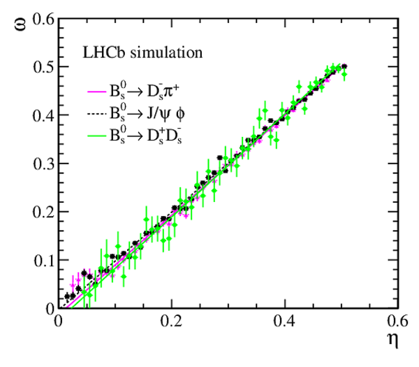
This ZIP file contains supplementary material for the publication LHCb-PAPER-2015-056. The files are: Supplementary.pdf: An overview of the extra figure *.pdf, *.png, *.eps, *.C: The figures in various formats. The *.C files contain the data on the figures.