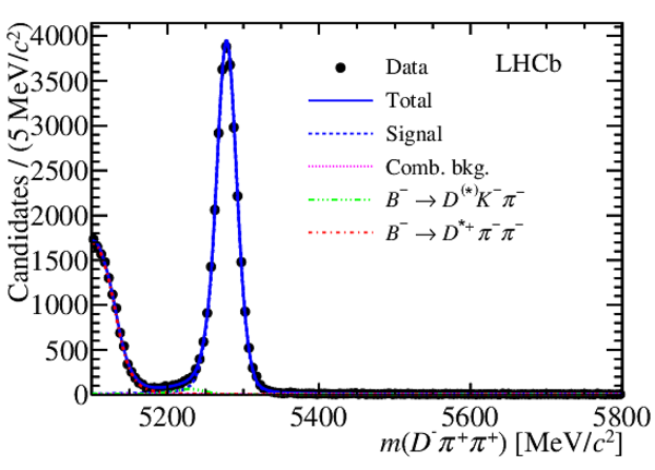
Results of the fit to the $B$ candidate invariant mass distribution shown with (left) linear and (right) logarithmic $y$-axis scales. Contributions are as described in the legend.

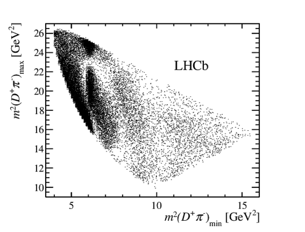
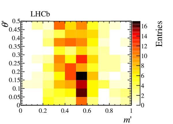
Distribution of $ B ^- \rightarrow D ^+ \pi ^- \pi ^- $ candidates in the signal region over (left) the DP and (right) the SDP.

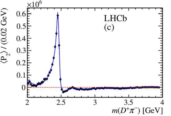
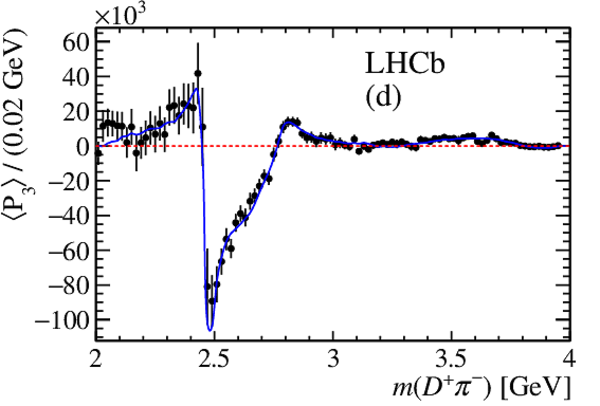
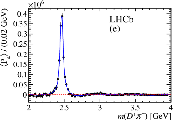
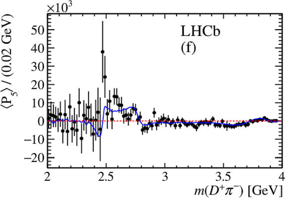
The first seven unnormalised angular moments for background-subtracted and efficiency-corrected data (black points) as a function of $m( D ^+ \pi ^- )$ in the range $2.0$--$4.0\mathrm{ Ge V} $. The blue line shows the result of the DP fit described in Sec. 7.

Unnormalised angular moments $\left\langle P_7 \right\rangle$ and $\left\langle P_8 \right\rangle$ for background-subtracted and efficiency-corrected data (black points) as a function of $m( D ^+ \pi ^- )$ in the range $2.0$--$4.0\mathrm{ Ge V} $. The blue line shows the result of the DP fit described in Sec. 7.

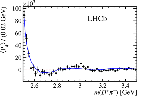
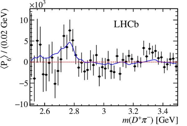
Zoomed views of the fourth and sixth unnormalised angular moments for background-subtracted and efficiency-corrected data (black points) as a function of $m( D ^+ \pi ^- )$. The blue line shows the result of the DP fit described in Sec. 7.

Signal efficiency across the SDP for $ B ^- \rightarrow D ^+ \pi ^- \pi ^- $ decays. The relative uncertainty at each point is typically $5 \%$.

Square Dalitz plot distributions for (left) combinatorial background and (right) $ B ^- \rightarrow D^{(*)+} K ^- \pi ^- $ decays.

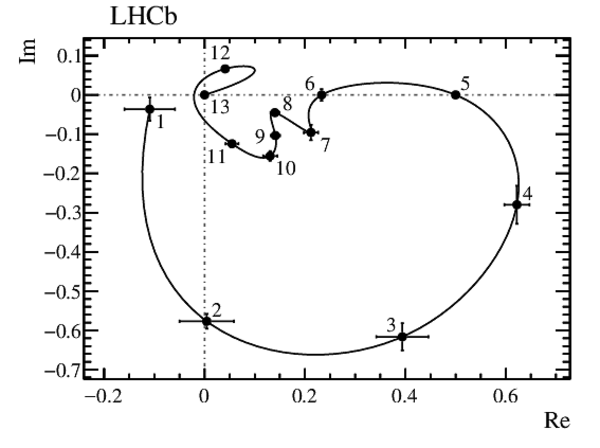
Real and imaginary parts of the S-wave amplitude, shown in an Argand diagram. The knots are shown with statistical uncertainties only, connected by the cubic spline interpolation used in the fit. The leftmost point is that at the lowest value of $m( D ^+ \pi ^- )$, with mass increasing along the connected points. Each point, labelled 1--13, corresponds to the position of a knot in the spline, at values of $m( D ^+ \pi ^- ) = \{ 2.01, 2.10, 2.20, 2.30, 2.40, 2.50, 2.60, 2.70, 2.80, 2.90, 3.10, 4.10, 5.14 \} \mathrm{ Ge V} $. The points at $(0.5,0.0)$ and $(0.0,0.0)$ are fixed. The anticlockwise rotation of the phase at low $m( D ^+ \pi ^- )$ is as expected due to the presence of the $ D ^{*}_{0}(2400)^{0}$ resonance.

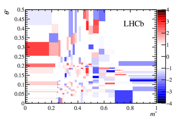
Differences between the SDP distribution of the data and fit model, in terms of the normalised residual in each bin. No bin lies outside the $z$-axis limits.

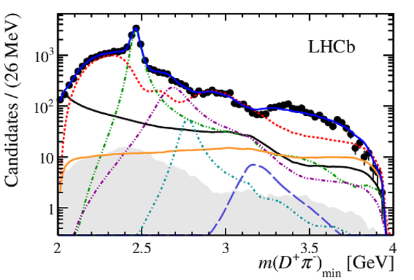
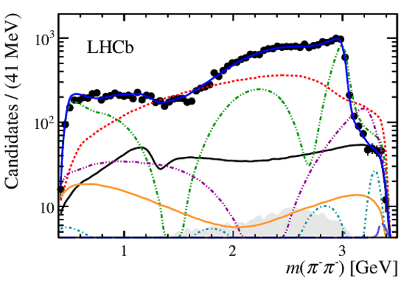
Projections of the data and amplitude fit onto (top) $m( D ^+ \pi ^- )_{\rm min}$, (middle) $m( D ^+ \pi ^- )_{\rm max}$ and (bottom) $m(\pi ^- \pi ^- )$, with the same projections shown (right) with a logarithmic $y$-axis scale. Components are described in the legend.

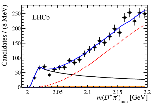
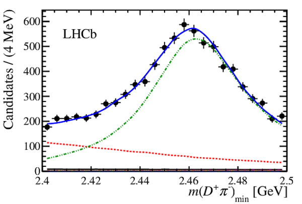
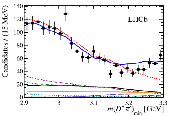
Projections of the data and amplitude fit onto (left) $m( D ^+ \pi ^- )$ and (right) the cosine of the helicity angle for the $ D ^+ \pi ^- $ system in (top to bottom) the low mass threshold region, the $ D ^{*}_{2}(2460)^{0}$ region, the $ D ^{*}_{1}(2680)^{0}$ -- $ D ^{*}_{3}(2760)^{0}$ region and the $ D ^{*}_{2}(3000)^{0}$ region. Components are as shown in Fig. 10.

Animated gif made out of all figures.

Measured properties of neutral excited charm states. World averages are given for the 1P resonances (top part), while all measurements are listed for the heavier states (bottom part). Where two uncertainties are given, the first is statistical and second systematic; where a third is given, it is due to model uncertainty. The uncertainties on the averages for the $ D ^{*}_{0}(2400)^{0}$ mass and the $D_1(2420)^0$ and $ D ^{*}_{2}(2460)^{0}$ masses and widths are inflated by scale factors to account for inconsistencies between measurements. The quoted $ D ^{*}_{2}(2460)^{0}$ averages do not include the recent result from Ref. [12].

Yields of the various components in the fit to $ B ^- \rightarrow D ^+ \pi ^- \pi ^- $ candidate invariant mass distribution. Note that the yields in the signal region are scaled from the full mass range.

Signal contributions to the fit model, where parameters and uncertainties are taken from Ref. [19]. States labelled with subscript $v$ are virtual contributions. The model "MIPW" refers to the quasi-model-independent partial wave approach.

Masses and widths determined in the fit to data, with statistical uncertainties only.

Complex coefficients and fit fractions determined from the Dalitz plot fit. Uncertainties are statistical only.

Breakdown of experimental systematic uncertainties on the fit fractions (%) and masses and widths $(\mathrm{Me V} )$.

Breakdown of model uncertainties on the fit fractions (%) and masses and widths $(\mathrm{Me V} )$.

Results for the complex amplitudes. The three quoted errors are statistical, experimental systematic and model uncertainties.

Results for the \DpiS-wave amplitude at the spline knots. The three quoted errors are statistical, experimental systematic and model uncertainties.

Results for the fit fractions. The three quoted errors are statistical, experimental systematic and model uncertainties.

Results for the product branching fractions ${\cal B}( B ^- \rightarrow R\pi ^- ) \times {\cal B}(R \rightarrow D ^+ \pi ^- )$. The four quoted errors are statistical, experimental systematic, model and inclusive branching fraction uncertainties.

Interference fit fractions (%) and statistical uncertainties. The amplitudes are: ($A_0$) $ D ^{*}_{v}(2007)^{0}$ , ($A_1$) \DpiS-wave , ($A_2$) $ D ^{*}_{2}(2460)^{0}$ , ($A_3$) $ D ^{*}_{1}(2680)^{0}$ , ($A_4$) $B^{*0}_v$, ($A_5$) $ D ^{*}_{3}(2760)^{0}$ , ($A_6$) $ D ^{*}_{2}(3000)^{0}$ . The diagonal elements are the same as the conventional fit fractions.

(Top) Experimental and (bottom) model systematic uncertainties on the interference fit fractions (%). The amplitudes are: ($A_0$) $ D ^{*}_{v}(2007)^{0}$ , ($A_1$) \DpiS-wave , ($A_2$) $ D ^{*}_{2}(2460)^{0}$ , ($A_3$) $ D ^{*}_{1}(2680)^{0}$ , ($A_4$) $B^{*0}_{v}$, ($A_5$) $ D ^{*}_{3}(2760)^{0}$ , ($A_6$) $ D ^{*}_{2}(3000)^{0}$ . The diagonal elements are the same as the conventional fit fractions.