Observation of the decay $B^0_s \to \phi\pi^+\pi^-$ and evidence for $B^0 \to \phi\pi^+\pi^-$

Information

LHCb-PAPER-2016-028
CERN-EP-2016-213
arXiv:1610.05187 [PDF]

(Submitted on 17 Oct 2016)
Phys. Rev. D95 (2017) 012006
Inspire 1492324

Tools

Abstract

The first observation of the rare decay$B^0_s \to \phi\pi^+\pi^-$ and evidence for $B^0 \to \phi\pi^+\pi^-$ are reported, using $pp$ collision data recorded by the LHCb detector at centre-of-mass energies $\sqrt{s} = 7$ and 8 TeV, corresponding to an integrated luminosity of $3{ fb^{-1}}$. The branching fractions in the $\pi^+\pi^-$ invariant mass range $400<m(\pi^+\pi^-)<1600{\mathrm{ Me V /}c^2}$ are $[3.48\pm 0.23\pm 0.17\pm 0.35]\times 10^{-6}$ and $[1.82\pm 0.25\pm 0.41\pm 0.14]\times 10^{-7}$ for $B^0_s \to \phi\pi^+\pi^-$ and $B^0 \to \phi\pi^+\pi^-$ respectively, where the uncertainties are statistical, systematic and from the normalisation mode $B^0_s \to \phi\phi $. A combined analysis of the $\pi^+\pi^-$ mass spectrum and the decay angles of the final-state particles identifies the exclusive decays $B^0_s \to \phi f_0(980) $, $B_s^0 \to \phi f_2(1270) $, and $B^0_s \to \phi\rho^0$ with branching fractions of $[1.12\pm 0.16^{+0.09}_{-0.08}\pm 0.11]\times 10^{-6}$, $[0.61\pm 0.13^{+0.12}_{-0.05}\pm 0.06]\times 10^{-6}$ and $[2.7\pm 0.7\pm 0.2\pm 0.2]\times 10^{-7}$, respectively.

Figures and captions

Feynman diagrams for the exclusive decays (a) $B_s^0 \rightarrow \phi f _{0}(980) $ and (b) $B_s^0 \rightarrow \phi \rho^0$.	fig1a.pdf [15 KiB] HiDef png [46 KiB] Thumbnail [22 KiB] *.C file
	fig1b.pdf [12 KiB] HiDef png [31 KiB] Thumbnail [15 KiB] *.C file
The $ K^+ K^- \pi^+ \pi^-$ invariant mass distribution for candidates in the mass range $0.4 < m_{\pi\pi} < 1.6$ $ {\mathrm{ Ge V /}c^2}$ . The fit described in the text is overlaid. The solid (red) line is the total fitted function, the dotted (green) line the combinatorial background, the dashed (blue) line the $ B ^0_ s $ and the dot-dashed (black) line the $ B ^0 $ signal component.	fig2.pdf [20 KiB] HiDef png [170 KiB] Thumbnail [132 KiB] *.C file
The $K^+ K^- K^+ K^-$ invariant mass distribution after all selection criteria. The solid (red) line is the total fitted function including the $ B ^0_ s \rightarrow \phi \phi$ signal, and the dashed (green) line is the combinatorial background.	fig3.pdf [19 KiB] HiDef png [176 KiB] Thumbnail [141 KiB] *.C file
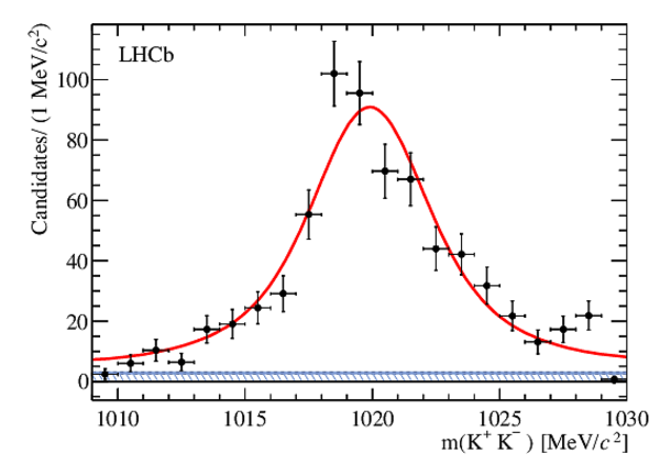
The $ K^+ K^- $ invariant mass distribution for background-subtracted $ B ^0_ s \rightarrow \phi \pi ^+ \pi ^- $ signal events with a fit to the dominant P-wave $\phi$ meson shown as a solid (red) line, and a small S-wave $ K^+ K^- $ contribution shown as a hatched (blue) area.	fig4.pdf [12 KiB] HiDef png [183 KiB] Thumbnail [150 KiB] *.C file
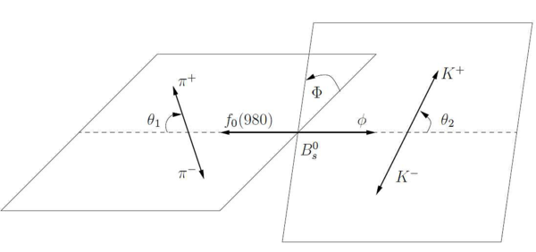
The definition of the decay angles $\theta_1$, $\theta_2$ and $\Phi$ for the decay $ B ^0_ s \rightarrow \phi \pi ^+ \pi ^- $ with $\phi\rightarrow K^+K^-$ and taking $f_0(980)\rightarrow \pi^+\pi^-$ for illustration.	fig5.pdf [27 KiB] HiDef png [253 KiB] Thumbnail [105 KiB] *.C file
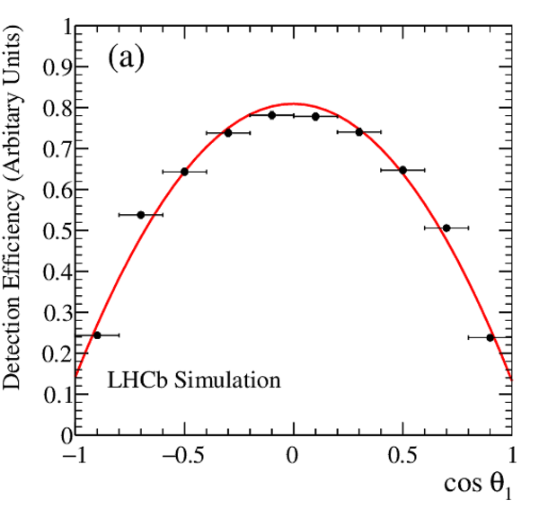
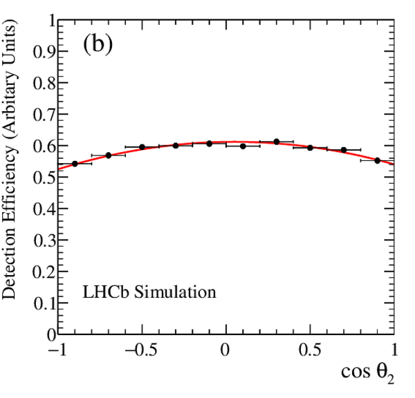
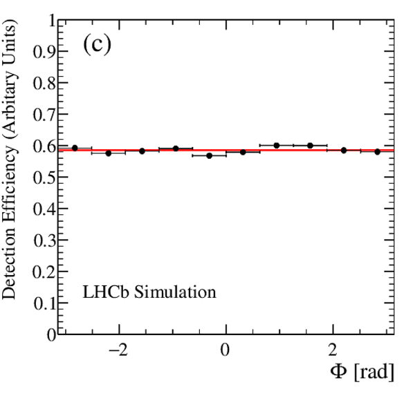
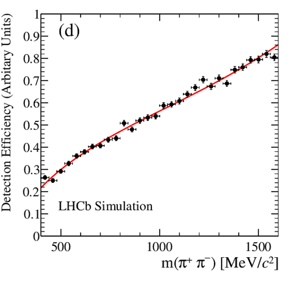
One-dimensional projections of the detection efficiency parameterised using Legendre polynomials (solid red lines) as a function of (a) $\cos\theta_1$, (b) $\cos\theta_2$, (c) $\Phi$ and (d) $m(\pi^+ \pi^- )$, superimposed on the efficiency determined from the ratio of the accepted/generated $ B ^0_ s \rightarrow \phi \pi ^+ \pi ^- $ events.	fig6a.pdf [15 KiB] HiDef png [180 KiB] Thumbnail [162 KiB] *.C file
	fig6b.pdf [15 KiB] HiDef png [158 KiB] Thumbnail [148 KiB] *.C file
	fig6c.pdf [14 KiB] HiDef png [134 KiB] Thumbnail [133 KiB] *.C file
	fig6d.pdf [17 KiB] HiDef png [197 KiB] Thumbnail [181 KiB] *.C file
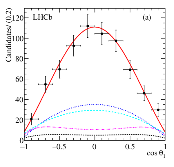
Projections of (a) $\cos\theta_1$, (b) $\cos\theta_2$, (c) $\Phi$, and (d) $m(\pi^+ \pi^- )$ for the preferred fit. The $\rho$ contribution is shown by the dotted (black) line, the $f_0(980)$ by the dot-dashed (blue) line, the $f_2(1270)$ by the double-dot-dashed (magenta) line and the $f_0(1500)$ by the dashed (cyan) line. Note that the expected distributions from each resonance include the effect of the experimental efficiency. The solid (red) line shows the total fit. The points with error bars are the data, where the background has been subtracted using the $ B ^0_ s $ signal weights from the $ K^+ K^- \pi^+ \pi^- $ invariant mass fit.	fig7a.pdf [16 KiB] HiDef png [208 KiB] Thumbnail [169 KiB] *.C file
	fig7b.pdf [15 KiB] HiDef png [228 KiB] Thumbnail [184 KiB] *.C file
	fig7c.pdf [10 KiB] HiDef png [167 KiB] Thumbnail [145 KiB] *.C file
	fig7d.pdf [20 KiB] HiDef png [293 KiB] Thumbnail [228 KiB] *.C file
Animated gif made out of all figures.	PAPER-2016-028.gif Thumbnail

Tables and captions

Possible resonances contributing to the $m(\pi^+ \pi^- )$ mass distribution. The shapes are either relativistic Breit-Wigner (BW) functions, or empirical threshold functions for the $f_0(500)$ proposed by Bugg [26] based on data from BES, and for the $f_0(980)$ proposed by Flatt\'e [27] to account for the effect of the $ K^+ K^- $ threshold.	Table_1.pdf [33 KiB] HiDef png [90 KiB] Thumbnail [43 KiB] tex code
The individual terms $i=1$ to $i=6$ come from the S-wave and P-wave $\pi^+ \pi^- $ amplitudes associated with the $f_0(980)$ and $\rho$, and the terms $i=7$ to $i=12$ come from the D-wave amplitudes associated with the $f_2(1270)$. See the text for definitions of $T_i$, $f_i$ and $\mathcal{M}_i$, and for a discussion of the interference terms omitted from this table.	Table_2.pdf [71 KiB] HiDef png [115 KiB] Thumbnail [49 KiB] tex code
The resonance amplitudes and phases from the preferred fit to the $m(\pi^+ \pi^- )$ and decay angle distributions of the $ B ^0_ s $ candidates, including the $\rho$, $f_0(980)$, $f_2(1270)$ and $f_0(1500)$. See text for definitions of the amplitudes and phases.	Table_3.pdf [52 KiB] HiDef png [87 KiB] Thumbnail [44 KiB] tex code
Fit fractions in % and event yields for the resonances contributing to $ B ^0_ s \rightarrow \phi \pi ^+ \pi ^- $. Results are quoted for the preferred model with a $\rho$, and for an alternative model without a $\rho$ which is used to evaluate systematic uncertainties.	Table_4.pdf [38 KiB] HiDef png [60 KiB] Thumbnail [31 KiB] tex code
Selection efficiencies for the signal and normalisation modes in %, as determined from simulated event samples. Here "Initial selection" refers to a loose set of requirements on the four tracks forming the $ B $ candidate. The "Offline selection" includes the charm and $\phi K^*{^0}$ vetoes, as well as the BDT. Angular acceptance and decay time refer to corrections made for the incorrect modelling of these distributions in the inclusive and $ B ^0_ s \rightarrow \phi f _{0}(980) $ simulated event samples.	Table_5.pdf [54 KiB] HiDef png [64 KiB] Thumbnail [27 KiB] tex code
Systematic uncertainties in % on the branching fractions of $ B ^0_ s $ and $ B ^0$ decays. All the uncertainties are taken on the ratio of the signal to the normalisation mode. Uncertainties marked by a dash are either negligible or exactly zero. The asymmetric uncertainties on $\phi f_0(980)$ and $\phi f_2(1270)$ come from the differences in yields between the fits with and without the $\rho^0$ contribution.	Table_6.pdf [56 KiB] HiDef png [67 KiB] Thumbnail [29 KiB] tex code