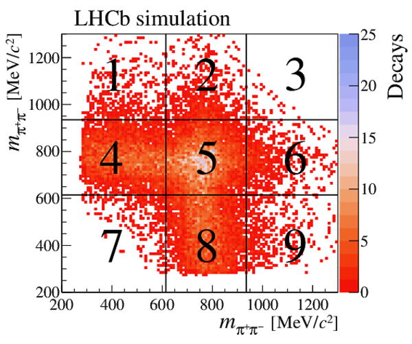
Two-dimensional distribution of the invariant masses $m_{\pi ^+ \pi ^- }$ of the two oppositely charged two-pion combinations for simulated $ B ^0_ s \rightarrow \tau ^+\tau ^- $ candidates. The distribution is symmetric by construction. The vertical and horizontal lines illustrate the sector boundaries.

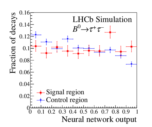
(left) Normalised NN output distribution in the signal ($\widehat{\mathcal{N}}^{\text{SR}}_{\text{sim}}$) and control ($\widehat{\mathcal{N}}^{\text{CR}}_{\text{sim}}$) region for $ B ^0_ s \rightarrow \tau ^+\tau ^- $ simulated events. (right) Normalised NN output distribution in the data control region $\widehat{\mathcal{N}}^{\text{CR}}_{\text{data}}$. The uncertainties reflect the statistics of the (simulated) data.

Distribution of the NN output in the signal region $\mathcal{N}^{\text{SR}}_{\text{data}}$ (black points), with the total fit result (blue line) and the background component (green line). The fitted $ B ^0_ s \rightarrow \tau ^+\tau ^- $ signal component is negative and is therefore shown multiplied by $-1$ (red line). For each bin of the signal and background component the combined statistical and systematic uncertainty on the template is shown as a light-coloured band. The difference between data and fit divided by its uncertainty (pull) is shown underneath.

Invariant mass distribution of the reconstructed $ B ^0 \rightarrow D^-D_s^{+}$ candidates in data (black points), together with the total fit result (blue line) used to determine the $ B ^0 \rightarrow D^-D_s^{+}$ yield. The individual components are described in the text.

Distribution of the NN output in the signal region $\mathcal{N}^{\text{SR}}_{\text{data}}$ (black points), with the total fit result (blue line), and the background component (green line). Shown is the fit using the "background only" model. For each bin of the background component the combined statistical and systematic uncertainty is shown as a light-coloured band. The difference between data and fit divided by its uncertainty (pull) is shown underneath.

Profile likelihood scan of the $ B ^0_ s \rightarrow \tau ^+\tau ^- $ signal yield. The intersections of the likelihood curve with the horizontal lines define the 68.3%, 95.4% and 99.7% likelihood intervals.

The $p$-value derived with the CL$_{\text{s}}$ method as a function of $\mathcal{B} ( B ^0_ s \rightarrow \tau ^+\tau ^- )$. Expected (observed) values are shown by a dashed (full) black line. The green (yellow) band covers the regions of 68% and 95% confidence for the expected limit. The red horizontal line corresponds to the limit at 95% CL.

Normalised NN output distribution in the signal ($\widehat{\mathcal{N}}^{\text{SR}}_{\text{sim}}$) and control ($\widehat{\mathcal{N}}^{\text{CR}}_{\text{sim}}$) region for $ B ^0 \rightarrow \tau ^+\tau ^- $ simulated events.

Fit results for $ B ^0 \rightarrow \tau ^+\tau ^- $. Distribution $\mathcal{N}^{\text{SR}}_{\text{data}}$ (black points), overlaid with the total fit result (blue line), and background component (green line), assuming all signal events originate from $ B ^0 \rightarrow \tau ^+\tau ^- $ decays. The $ B ^0 \rightarrow \tau ^+\tau ^- $ signal component is also shown (red line), multiplied by $-1$. For each bin of the signal and background component the combined statistical and systematic uncertainty is shown as a light-coloured band. The difference between data and fit divided by its uncertainty (pull) is shown underneath.

The $p$-value derived with the CL$_{\text{s}}$ method as a function of $\mathcal{B} ( B ^0 \rightarrow \tau ^+\tau ^- $). Expected (observed) values are shown by a dashed (full) black line. The green (yellow) band covers the regions of 68% and 95% confidence for the expected limit. The red horizontal line corresponds to the limit at 95% CL.

Animated gif made out of all figures.

Supplementary material full pdf

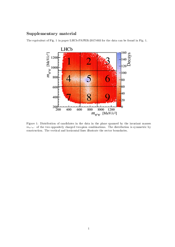
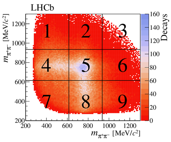
This ZIP file contains supplemetary material for the publication LHCb-PAPER-2017-003. The files are: supplementary.pdf : An overview of the extra figures *.pdf, *.png, *.eps, *.C : The figures in various formats