Measurement of the shape of the $ {B}_s^0\to {D}_s^{\ast -}{\mu}^{+}{\nu}_{\mu } $ differential decay rate

Information

LHCb-PAPER-2019-046
CERN-EP-2020-026
arXiv:2003.08453 [PDF]

(Submitted on 18 Mar 2020)
JHEP 12 (2020) 144
Inspire 1787090

Tools

Abstract

The shape of the $B_s^0\rightarrow D_s^{*-}\mu^+\nu_{\mu}$ differential decay rate is obtained as a function of the hadron recoil using proton-proton collision data at a centre-of-mass energy of 13 TeV, corresponding to an integrated luminosity of 1.7 fb$^{-1}$ collected by the LHCb detector. The $B_s^0\rightarrow D_s^{*-}\mu^+\nu_{\mu}$ decay is reconstructed through the decays $D_s^{*-}\rightarrow D_s^{-}\gamma$ and $D_s^{-}\rightarrow K^-K^+\pi^-$. The differential decay rate is fitted with the Caprini-Lellouch-Neubert (CLN) and Boyd-Grinstein-Lebed (BGL) parametrisations of the form factors, and the relevant quantities for both are extracted.

Figures and captions

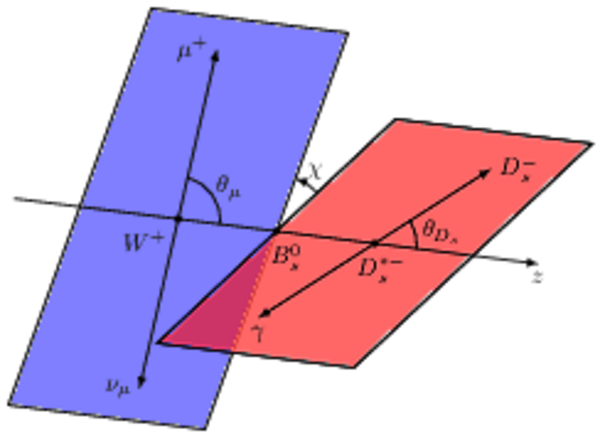
Schematic overview of the $ B ^0_ s \rightarrow D ^{*-}_ s \mu ^+ \nu _\mu $ decay, introducing the angles $\theta_{D_s}$ , $\theta_{\mu}$ and $\chi$.	Fig1.pdf [40 KiB] HiDef png [328 KiB] Thumbnail [236 KiB] *.C file
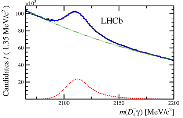
Distribution of the reconstructed $ D ^-_ s \gamma $ mass, $m( D ^-_ s \gamma )$, with the fit overlaid. The fit is performed constraining the $ D ^-_ s $ mass to the world-average value [16]. The signal and background components are shown separately with dashed red and dotted green lines, respectively.	Fig2.pdf [25 KiB] HiDef png [170 KiB] Thumbnail [131 KiB] *.C file
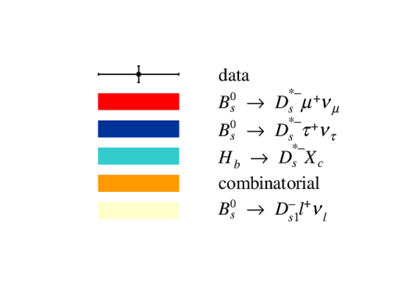
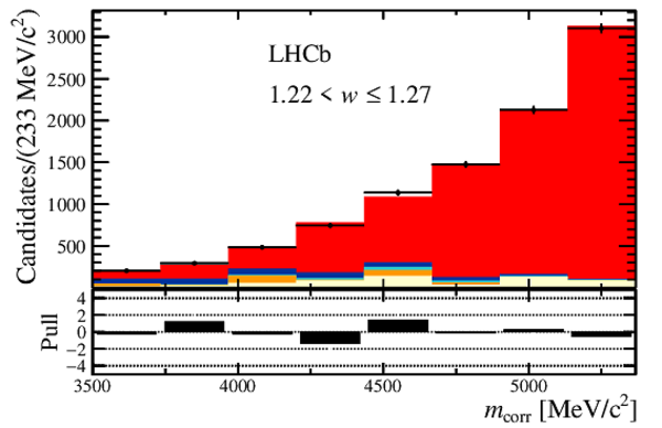
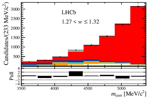
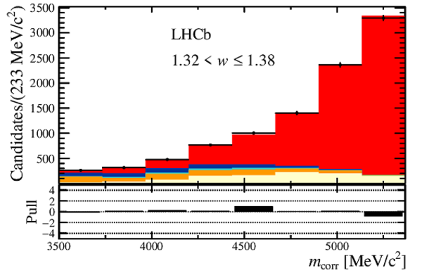
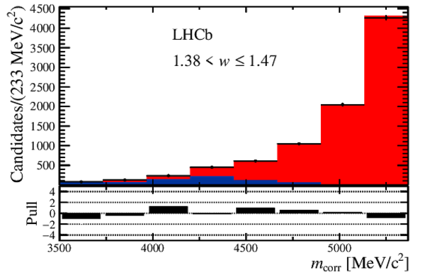
Distribution of the corrected mass, $m_{\rm corr}$, for the seven bins of $ w$ , overlaid with the fit results. The $ B ^0_ s \rightarrow D _{ s 1}(2460)^- \tau ^+ \nu _\tau $ and the $ B ^0_ s \rightarrow D _{ s 1}(2460)^- \mu ^+ \nu _\mu $ components are combined in $ B ^0_ s \rightarrow D _{ s 1}(2460)^- \ell^+ \nu _\ell $ . Below each plot, differences between the data and fit are shown, normalised by the uncertainty in the data.	Fig3a.pdf [13 KiB] HiDef png [71 KiB] Thumbnail [60 KiB] *.C file
	Fig3b.pdf [15 KiB] HiDef png [182 KiB] Thumbnail [156 KiB] *.C file
	Fig3c.pdf [15 KiB] HiDef png [178 KiB] Thumbnail [149 KiB] *.C file
	Fig3d.pdf [15 KiB] HiDef png [178 KiB] Thumbnail [153 KiB] *.C file
	Fig3e.pdf [15 KiB] HiDef png [177 KiB] Thumbnail [148 KiB] *.C file
	Fig3f.pdf [15 KiB] HiDef png [175 KiB] Thumbnail [149 KiB] *.C file
	Fig3g.pdf [15 KiB] HiDef png [180 KiB] Thumbnail [154 KiB] *.C file
	Fig3h.pdf [15 KiB] HiDef png [183 KiB] Thumbnail [157 KiB] *.C file
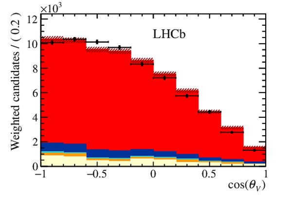
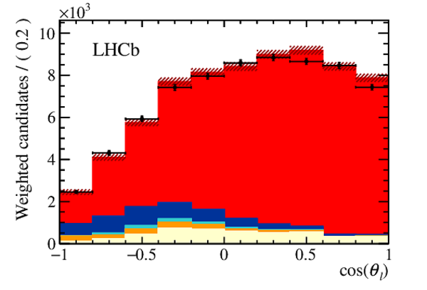
Distribution of (top right) $\chi$, (bottom left) $\cos(\theta_{D_s} )$ and (bottom right) $\cos(\theta_{\mu} )$ integrating over $w$ and the other decay angles from data (black points) compared to the distribution from simulation with their relative size extracted from the fit to the corrected mass. The $ B ^0_ s \rightarrow D _{ s 1}(2460)^- \tau ^+ \nu _\tau $ and the $ B ^0_ s \rightarrow D _{ s 1}(2460)^- \mu ^+ \nu _\mu $ components are combined in $ B ^0_ s \rightarrow D _{ s 1}(2460)^- \ell^+ \nu _\ell $ . The uncertainties on the templates, indicated by the hashed areas in the figures, are a combination from all templates.	Fig3a.pdf [13 KiB] HiDef png [71 KiB] Thumbnail [60 KiB] *.C file
	Fig4a.pdf [16 KiB] HiDef png [179 KiB] Thumbnail [126 KiB] *.C file
	Fig4b.pdf [16 KiB] HiDef png [166 KiB] Thumbnail [122 KiB] *.C file
	Fig4c.pdf [16 KiB] HiDef png [171 KiB] Thumbnail [121 KiB] *.C file
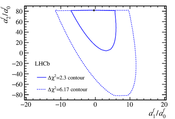
$\Delta$ $\chi^2$ contours for the scaled parameters $a_1^f/a_0^f$ versus $a_2^f/a_0^f$. The black cross marks the best-fit central value. The solid (dashed) contour encloses the $\Delta$ $\chi^2$ = 2.3 (6.17) region. The observed shape is due to the applied unitarity condition, see Eq. ???.	Fig5.pdf [15 KiB] HiDef png [145 KiB] Thumbnail [132 KiB] *.C file
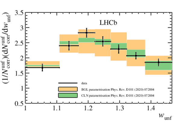
Unfolded normalised differential decay rate with the fit superimposed for the CLN parametrisation (green), and BGL (red). The band in the fit results includes both the statistical and systematic uncertainty on the data yields.	Fig6.pdf [26 KiB] HiDef png [281 KiB] Thumbnail [188 KiB] *.C file
Total efficiency as a function of $ w_{\rm true}$ , including the acceptance of the LHCb detector as well as the reconstruction and selection efficiencies.	Fig7.pdf [14 KiB] HiDef png [68 KiB] Thumbnail [43 KiB] *.C file
$\Delta$ $\chi^2$ contours for the scaled parameters $a_1^f$ versus $a_2^f$. The black cross marks the best-fit central value. The solid (dashed) contour encloses the $\Delta$ $\chi^2$ = 2.3 (6.17) region. The observed shape is due to the applied unitarity condition, see Eq. 11.	Fig8.pdf [15 KiB] HiDef png [123 KiB] Thumbnail [109 KiB] *.C file
Comparison between the $ w$ spectrum measured in this paper to the normalised $\Delta\Gamma/\Delta w $ spectra inferred from the CLN and BGL parametrisations in Ref. [7].	Fig9.pdf [14 KiB] HiDef png [180 KiB] Thumbnail [142 KiB] *.C file
Animated gif made out of all figures.	PAPER-2019-046.gif Thumbnail

Tables and captions

Binning scheme used for this measurement. Only the upper bound for each bin is presented. The lower bound on the first bin corresponds to $w=1$.	Table_1.pdf [36 KiB] HiDef png [14 KiB] Thumbnail [6 KiB] tex code
Fraction of the unfolded yields corrected for the global efficiencies, $N^{\mathrm{unf}}_{\mathrm{corr}}$, for each $ w$ bin. Also shown in this table is the breakdown of the systematic and statistical uncertainties on $N^{\mathrm{unf}}_{\mathrm{corr}}$. These are shown as a fraction of the unfolded yield.	Table_2.pdf [67 KiB] HiDef png [116 KiB] Thumbnail [50 KiB] tex code
Correlation matrix for the unfolded data set in bins of $ w$ , including both statistical and systematic uncertainties.	Table_3.pdf [36 KiB] HiDef png [30 KiB] Thumbnail [12 KiB] tex code
Summary of the systematic and statistical uncertainties on the parameters $\rho^2$, $a_1^f$ and $a_2^f$ from the unfolded CLN and BGL fits. The total systematic uncertainty is obtained by adding the individual components in quadrature.	Table_4.pdf [67 KiB] HiDef png [103 KiB] Thumbnail [44 KiB] tex code
Results from different fit configurations, where the first uncertainty is statistical and the second systematic.	Table_5.pdf [70 KiB] HiDef png [63 KiB] Thumbnail [32 KiB] tex code
Covariance matrix for the unfolded data set in bins of $ w$ , including both statistical and systematic uncertainties in units of $10^{-5}$.	Table_6.pdf [50 KiB] HiDef png [36 KiB] Thumbnail [16 KiB] tex code
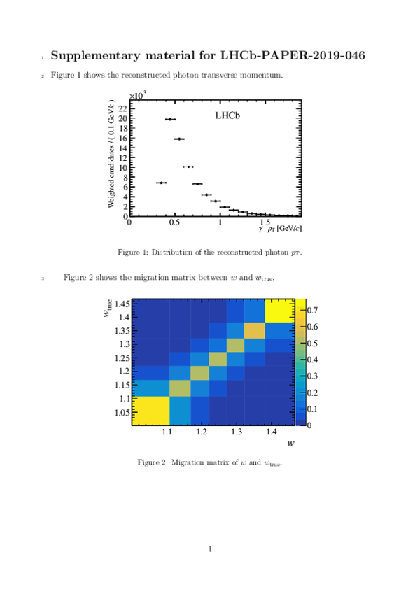
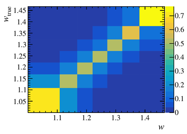
Response matrix, containing the migration from $ w_{\rm true}$ to $w$ bins together with the total efficiency in units of $10^{-4}$.	Table_7.pdf [57 KiB] HiDef png [50 KiB] Thumbnail [23 KiB] tex code
Fit inputs used for the BGL fit, taken from Ref. [17] and Ref. [24].	Table_8.pdf [75 KiB] HiDef png [107 KiB] Thumbnail [47 KiB] tex code

Supplementary Material [file]

Supplementary material full pdf	supple[..].pdf [119 KiB]
This ZIP file contains supplementary material for the publication LHCb-PAPER-2019-046. The files are: supplementary.pdf : An overview of the extra figures .pdf, .png, .eps, .C : The figures in various formats	Fig1-S.pdf [15 KiB] HiDef png [78 KiB] Thumbnail [46 KiB] *C file
	Fig2-S.pdf [14 KiB] HiDef png [136 KiB] Thumbnail [127 KiB] *C file
	Fig3-S.pdf [16 KiB] HiDef png [75 KiB] Thumbnail [44 KiB] *C file

Created on 27 April 2024.

The LHCb Public results

Measurement of the shape of the $ {B}_s^0\to {D}_s^{\ast -}{\mu}^{+}{\nu}_{\mu } $ differential decay rate

Information

LHCb-PAPER-2019-046

CERN-EP-2020-026

arXiv:2003.08453 [PDF]

(Submitted on 18 Mar 2020)

JHEP 12 (2020) 144

Inspire 1787090

Tools

Cited 25 times

Get BibTex

Rivet

Abstract

Figures and captions

Tables and captions

Supplementary Material [file]