

Compact Muon Solenoid
LHC, CERN
| CMS-BPH-13-007 ; LHCB-PAPER-2014-049 ; CERN-PH-EP-2014-220 | ||
| Observation of the rare $ B^0_s \to \mu^+\mu^-$ decay from the combined analysis of CMS and LHCb data | ||
| CMS and LHCb Collaborations | ||
| 17 November 2014 | ||
| Nature 522 (2015) 68 | ||
| Abstract: The standard model of particle physics describes the fundamental particles and their interactions via the strong, electromagnetic, and weak forces. It provides precise predictions for measurable quantities that can be tested experimentally. The probabilities, or branching fractions, of the strange B meson ($B^0_s$) and the $B^0$ meson decaying into two oppositely charged muons ($mu^+$ and $\mu^-$) are especially interesting because of their sensitivity to theories that extend the standard model. The standard model predicts that the $ B^0_s \to \mu^+ \mu^- $ and $ B^0 \to \mu^+ \mu^- $ decays are very rare, with about four of the former occurring for every billion $ B^0_s $ mesons produced and one of the latter occurring for every 10 billion $ B^0 $ mesons. A difference in the observed branching fractions with respect to the predictions of the standard model would provide a direction in which the standard model should be extended. Before the Large Hadron Collider (LHC) at CERN started operating, no evidence for either decay mode had been found. Upper limits on the branching fractions were an order of magnitude above the standard model predictions. The CMS (Compact Muon Solenoid) and LHCb (Large Hadron Collider beauty) collaborations have performed a joint analysis of the data from proton-proton collisions that they collected in 2011 at a centre-of-mass energy of seven teraelectronvolts and in 2012 at eight teraelectronvolts. Here we report the first observation of the $ B^0_s \to \mu^+ \mu^- $ decay, with a statistical signicance exceeding six standard deviations, and the best measurement so far of its branching fraction. Furthermore, we obtained evidence for the $ B^0 \to \mu^+ \mu^- $ decay with a statistical significance of three standard deviations. Both measurements are statistically compatible with standard model predictions and allow stringent constraints to be placed on theories beyond the standard model. The LHC experiments will resume data taking in 2015, recording proton-proton collisions at a centre-of-mass energy of 13 teraelectronvolts, which will approximately double the production rates for $ B^0_s $ and $ B^0 $ mesons and lead to further improvements in the precision of these crucial tests of the standard model. | ||
| Links: e-print arXiv:1411.4413 [hep-ex] (PDF) ; CDS record ; inSPIRE record ; Public twiki page ; CADI line (restricted) ; | ||
| Figures | |
png pdf |
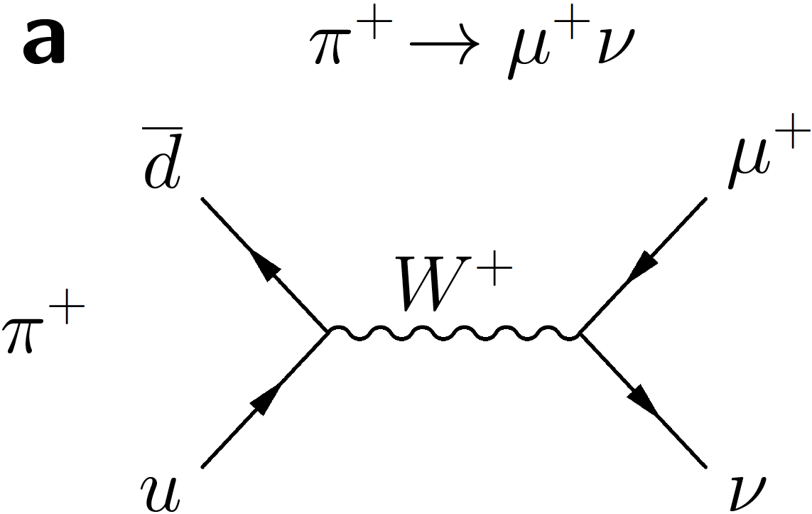
Figure 1-a:
Feynman diagrams for the $ B^0_{s} \rightarrow \mu ^+ \mu ^- $ and $ B^0 \rightarrow \mu^+ \mu ^- $ decays. Dominant processes in the SM (a,b,c,d) and example of processes in theories extending the SM (e,f,g), where new particles (NP) can contribute and potentially change the decay rate. |
png pdf |
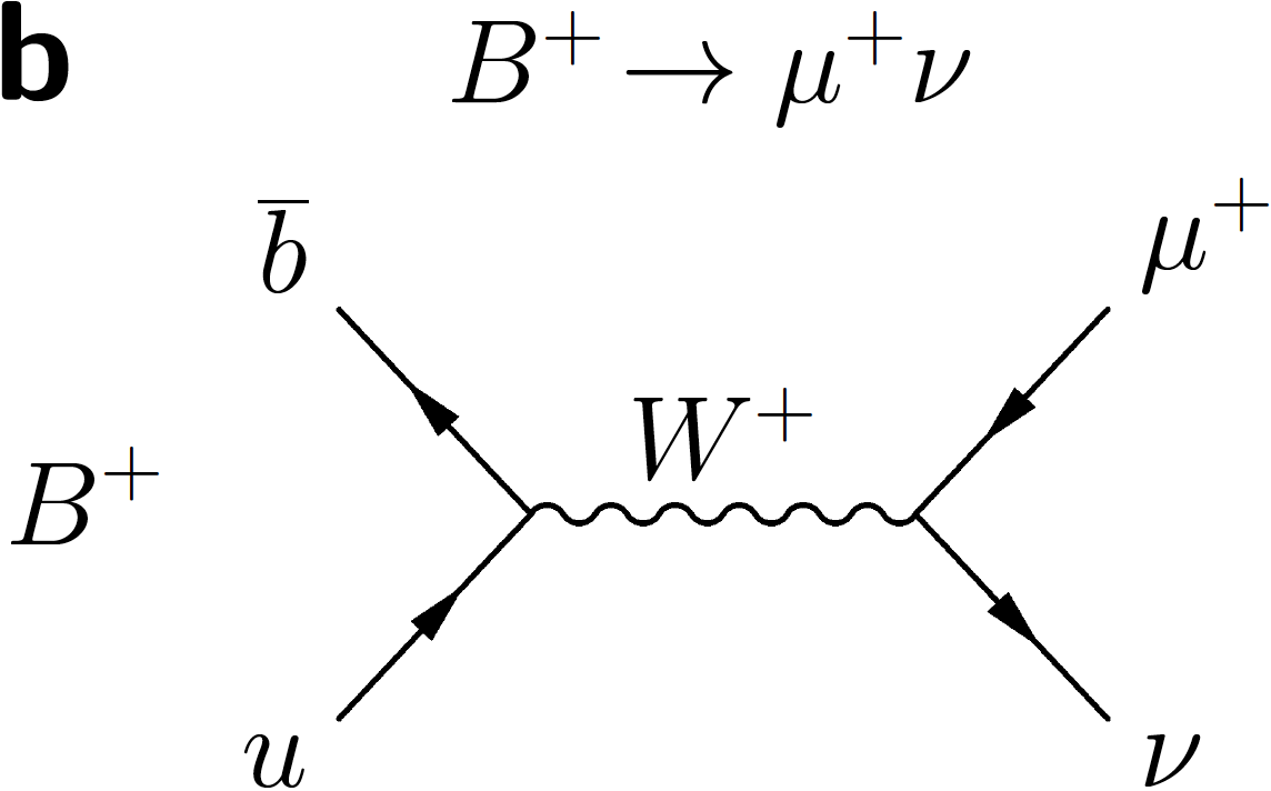
Figure 1-b:
Feynman diagrams for the $ B^0_{s} \rightarrow \mu ^+ \mu ^- $ and $ B^0 \rightarrow \mu^+ \mu ^- $ decays. Dominant processes in the SM (a,b,c,d) and example of processes in theories extending the SM (e,f,g), where new particles (NP) can contribute and potentially change the decay rate. |
png pdf |
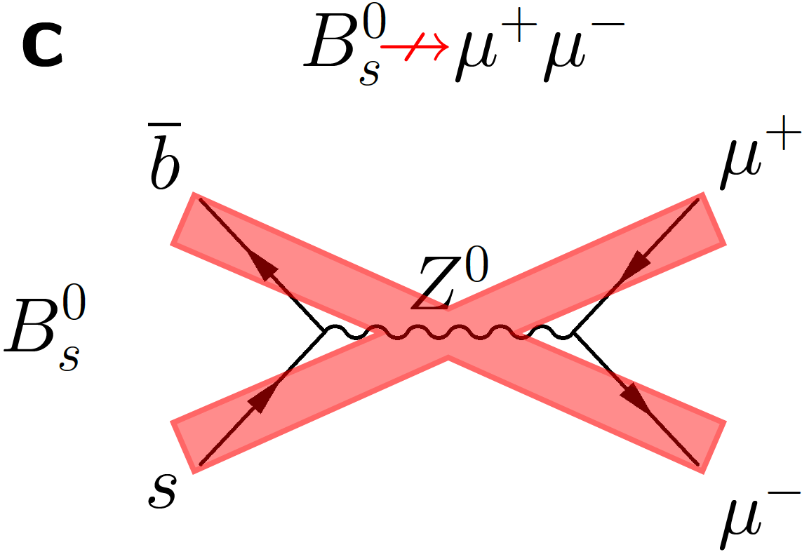
Figure 1-c:
Feynman diagrams for the $ B^0_{s} \rightarrow \mu ^+ \mu ^- $ and $ B^0 \rightarrow \mu^+ \mu ^- $ decays. Dominant processes in the SM (a,b,c,d) and example of processes in theories extending the SM (e,f,g), where new particles (NP) can contribute and potentially change the decay rate. |

png pdf |
Figure 1-d:
Feynman diagrams for the $ B^0_{s} \rightarrow \mu ^+ \mu ^- $ and $ B^0 \rightarrow \mu^+ \mu ^- $ decays. Dominant processes in the SM (a,b,c,d) and example of processes in theories extending the SM (e,f,g), where new particles (NP) can contribute and potentially change the decay rate. |
png pdf |
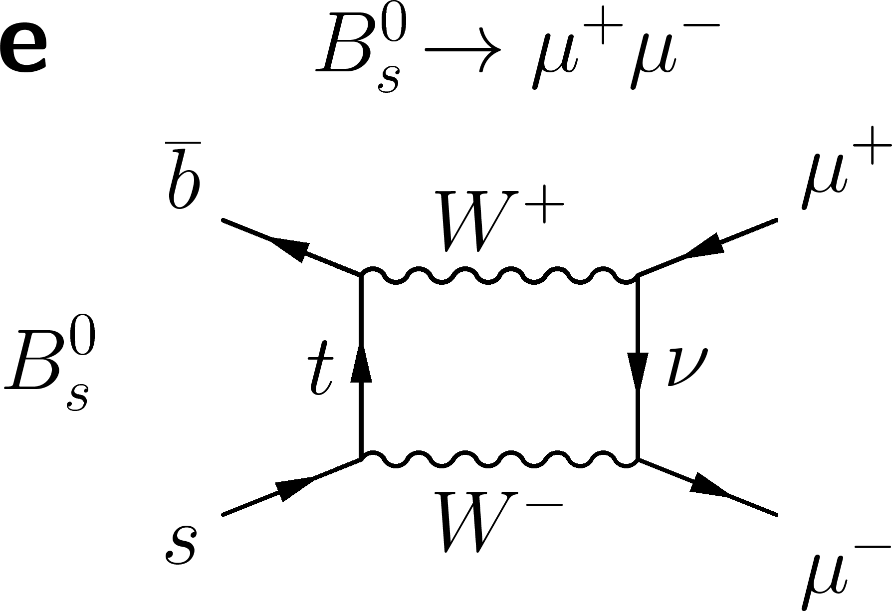
Figure 1-e:
Feynman diagrams for the $ B^0_{s} \rightarrow \mu ^+ \mu ^- $ and $ B^0 \rightarrow \mu^+ \mu ^- $ decays. Dominant processes in the SM (a,b,c,d) and example of processes in theories extending the SM (e,f,g), where new particles (NP) can contribute and potentially change the decay rate. |
png pdf |
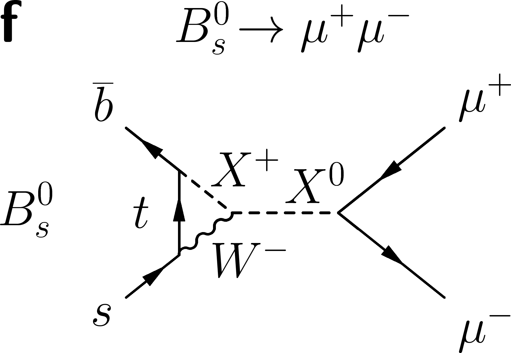
Figure 1-f:
Feynman diagrams for the $ B^0_{s} \rightarrow \mu ^+ \mu ^- $ and $ B^0 \rightarrow \mu^+ \mu ^- $ decays. Dominant processes in the SM (a,b,c,d) and example of processes in theories extending the SM (e,f,g), where new particles (NP) can contribute and potentially change the decay rate. |
png pdf |
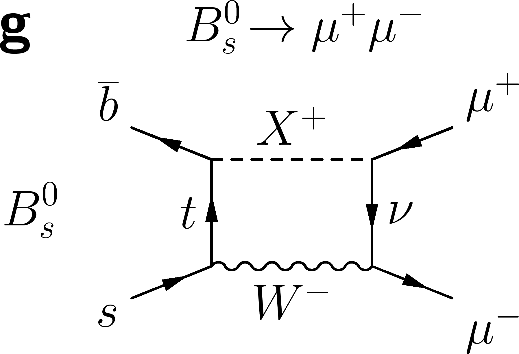
Figure 1-g:
Feynman diagrams for the $ B^0_{s} \rightarrow \mu ^+ \mu ^- $ and $ B^0 \rightarrow \mu^+ \mu ^- $ decays. Dominant processes in the SM (a,b,c,d) and example of processes in theories extending the SM (e,f,g), where new particles (NP) can contribute and potentially change the decay rate. |
png pdf |
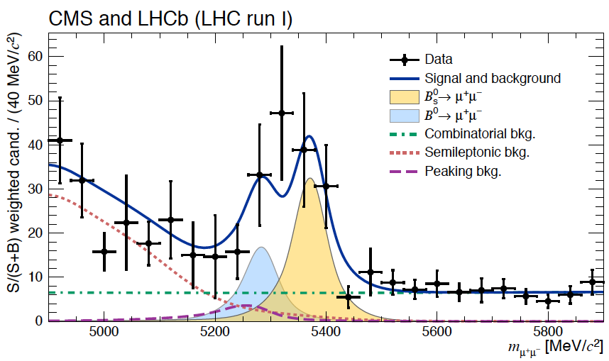
Figure 2:
Weighted distribution of the dimuon invariant mass, $m_{\mu^+ \mu^-}$, for all categories. Superimposed on the data points in black are the combined fit (solid blue line) and its components: the $B^0_s$ (yellow shaded area) and $B^0$ (light-blue shaded area) signal components; the combinatorial background (dash-dotted green line); the sum of the semi-leptonic backgrounds (dotted salmon line); and the peaking backgrounds (dashed violet line). The horizontal bar on each histogram point denotes the size of the binning, while the vertical bar denotes the 68% confidence interval. See main text for details on the weighting procedure. |

png pdf |
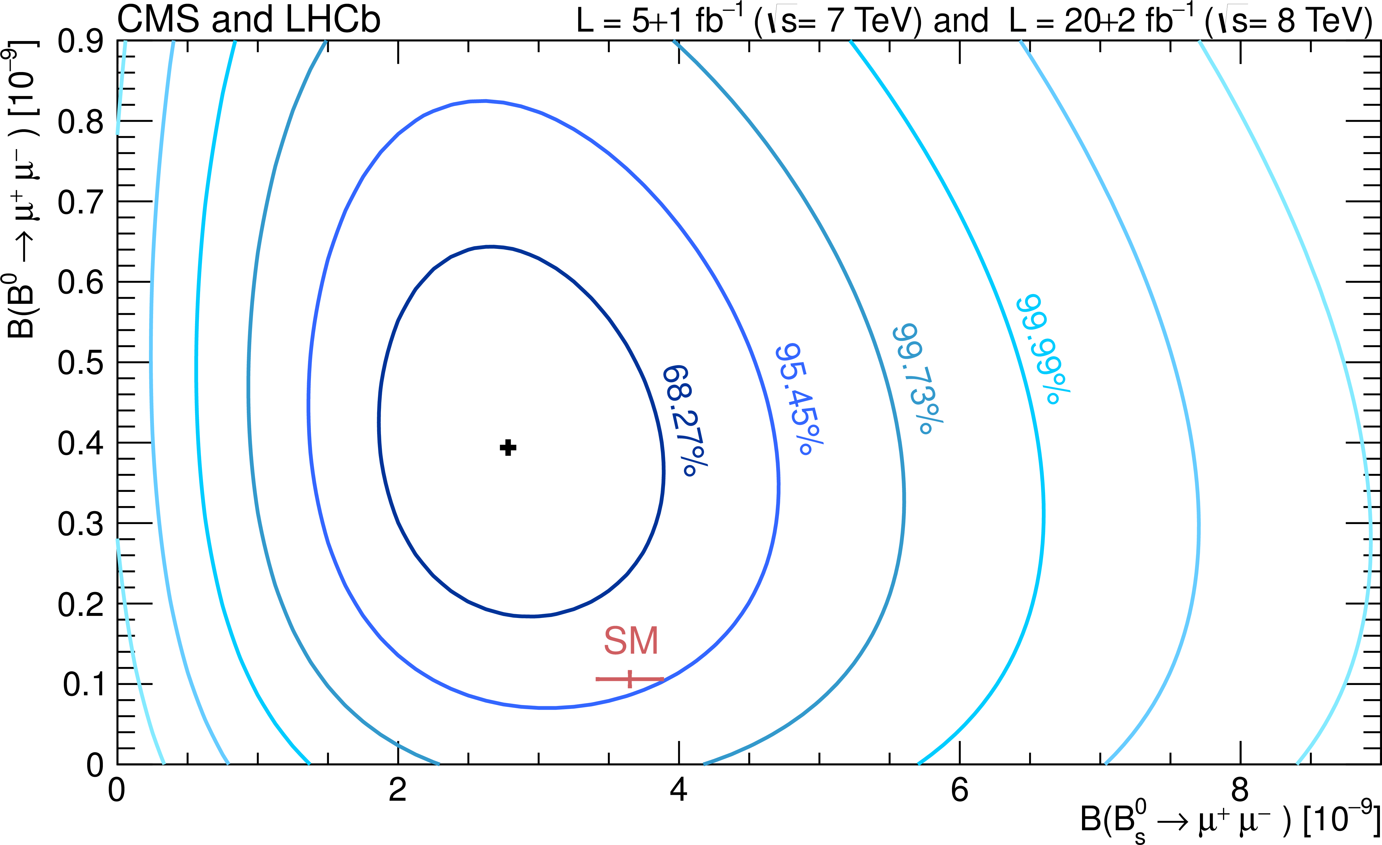
Figure 3:
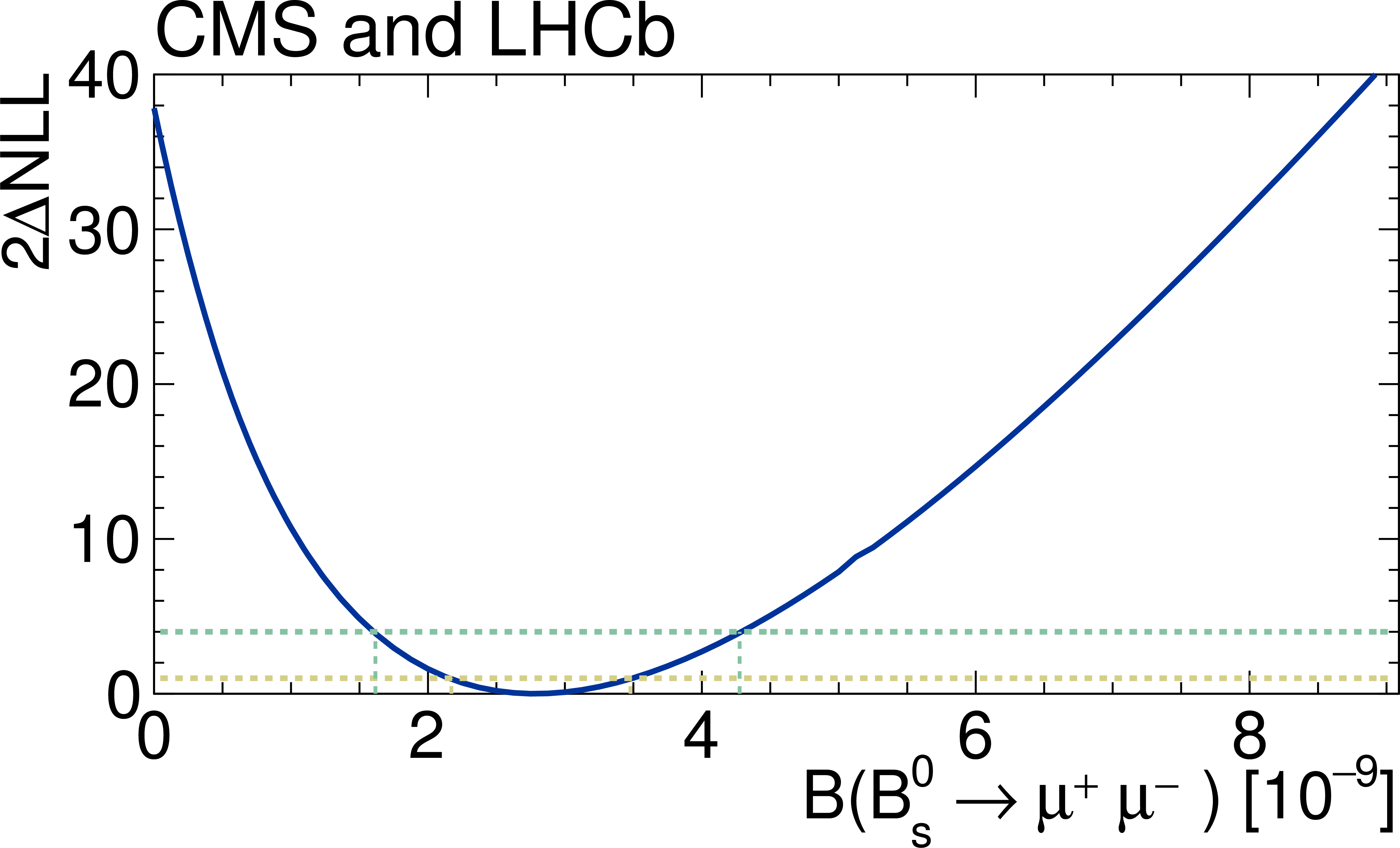
Likelihood contours in the $ \mathcal{B}( B^0 \to \mu^+ \mu^- ) $ versus $ \mathcal{B}( B^0_s \to \mu^+ \mu^- ) $ plane. The (black) cross in (a) marks the best-fit central value. The SM expectation and its uncertainty is shown as the (red) marker. Each contour encloses a region approximately corresponding to the reported confidence level. b, c: Variations of the test statistic $-2\Delta \ln L $ for $ \mathcal{B}( B^0_s \to \mu^+ \mu^- ) $ (b) and $ \mathcal{B}( B^0 \to \mu^+ \mu^- ) $ (c). The dark and light (cyan) areas define the $\pm 1 \sigma$ and $\pm 2 \sigma$ confidence intervals for the branching fraction, respectively. The SM prediction and its uncertainty for each branching fraction is denoted with the vertical (red) band. |
png pdf |
Figure 3-a:
Likelihood contours in the $ \mathcal{B}( B^0 \to \mu^+ \mu^- ) $ versus $ \mathcal{B}( B^0_s \to \mu^+ \mu^- ) $ plane. The (black) cross in (a) marks the best-fit central value. The SM expectation and its uncertainty is shown as the (red) marker. Each contour encloses a region approximately corresponding to the reported confidence level. b, c: Variations of the test statistic $-2\Delta \ln L $ for $ \mathcal{B}( B^0_s \to \mu^+ \mu^- ) $ (b) and $ \mathcal{B}( B^0 \to \mu^+ \mu^- ) $ (c). The dark and light (cyan) areas define the $\pm 1 \sigma$ and $\pm 2 \sigma$ confidence intervals for the branching fraction, respectively. The SM prediction and its uncertainty for each branching fraction is denoted with the vertical (red) band. |
png pdf |
Figure 3-b:
Likelihood contours in the $ \mathcal{B}( B^0 \to \mu^+ \mu^- ) $ versus $ \mathcal{B}( B^0_s \to \mu^+ \mu^- ) $ plane. The (black) cross in (a) marks the best-fit central value. The SM expectation and its uncertainty is shown as the (red) marker. Each contour encloses a region approximately corresponding to the reported confidence level. b, c: Variations of the test statistic $-2\Delta \ln L $ for $ \mathcal{B}( B^0_s \to \mu^+ \mu^- ) $ (b) and $ \mathcal{B}( B^0 \to \mu^+ \mu^- ) $ (c). The dark and light (cyan) areas define the $\pm 1 \sigma$ and $\pm 2 \sigma$ confidence intervals for the branching fraction, respectively. The SM prediction and its uncertainty for each branching fraction is denoted with the vertical (red) band. |

png pdf |
Figure 3-c:
Likelihood contours in the $ \mathcal{B}( B^0 \to \mu^+ \mu^- ) $ versus $ \mathcal{B}( B^0_s \to \mu^+ \mu^- ) $ plane. The (black) cross in (a) marks the best-fit central value. The SM expectation and its uncertainty is shown as the (red) marker. Each contour encloses a region approximately corresponding to the reported confidence level. b, c: Variations of the test statistic $-2\Delta \ln L $ for $ \mathcal{B}( B^0_s \to \mu^+ \mu^- ) $ (b) and $ \mathcal{B}( B^0 \to \mu^+ \mu^- ) $ (c). The dark and light (cyan) areas define the $\pm 1 \sigma$ and $\pm 2 \sigma$ confidence intervals for the branching fraction, respectively. The SM prediction and its uncertainty for each branching fraction is denoted with the vertical (red) band. |

png pdf |
Figure 4:
Variation of the test statistic $-2\Delta \ln L $ as a function of the ratio of branching fractions $\mathcal{R} \equiv \mathcal{B}( B^0 \to \mu^+ \mu^- ) / \mathcal{B}( B^0_s \to \mu^+ \mu^- ) $. The dark and light (cyan) areas define the $\pm 1 \sigma$ and $\pm 2 \sigma$ confidence intervals for R, respectively. The value and uncertainty for $\mathcal{R}$ predicted in the SM, which is the same in BSM theories with the minimal flavour violation (MFV) property, is denoted with the vertical (red) band. |
| Summary |
| The combined analysis of data from CMS and LHCb, taking advantage of their full statistical power, establishes conclusively the existence of the $ B^0_s \to \mu^+ \mu^- $ decay and provides an improved measurement of its branching fraction. This concludes a search that started more than three decades ago (see Extended Data Fig. 7), and initiates a phase of precision measurements of the properties of this decay. It also produces a three standard deviation evidence for the $ B^0 \to \mu^+ \mu^- $ decay. The measured branching fractions of both decays are compatible with SM predictions. This is the first time that the CMS and LHCb collaborations have performed a combined analysis of sets of their data in order to obtain a statistically significant observation. |
|
|
Compact Muon Solenoid LHC, CERN |
|

|

|

|

|

|