

Compact Muon Solenoid
LHC, CERN
| CMS-BPH-13-010 ; CERN-PH-EP-2015-178 | ||
| Angular analysis of the decay $ \mathrm{ B^0 \to K^{*0} \mu^{+} \mu^{-} }$ from pp collisions at $\sqrt{s}= $ 8 TeV | ||
| CMS Collaboration | ||
| 29 July 2015 | ||
| Phys. Lett. B 753 (2016) 424 | ||
| Abstract: The angular distributions and the differential branching fraction of the decay $ \mathrm{ B^0 \to K^{*}(892)^0 \mu^{+} \mu^{-} }$ are studied using data corresponding to an integrated luminosity of 20.5 fb$^{-1}$ collected with the CMS detector at the LHC in pp collisions at $\sqrt{s} =$ 8 TeV. From 1430 signal decays, the forward-backward asymmetry of the muons, the $\mathrm{ K^{*}(892)^0 }$ longitudinal polarization fraction, and the differential branching fraction are determined as a function of the dimuon invariant mass squared. The measurements are among the most precise to date and are in good agreement with standard model predictions. | ||
| Links: e-print arXiv:1507.08126 [hep-ex] (PDF) ; CDS record ; inSPIRE record ; Public twiki page ; HepData record ; CADI line (restricted) ; | ||
| Figures | |
png pdf |
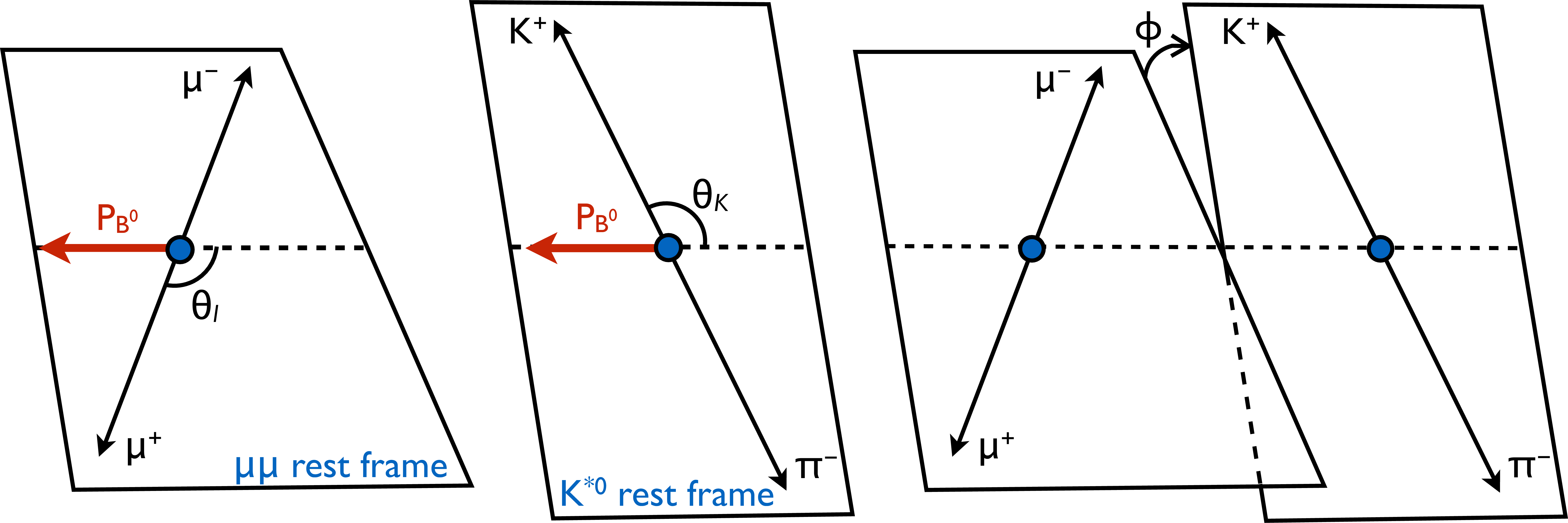
Figure 1:
Sketch showing the definition of the angular observables $\theta _l$ (a), $\theta _ {\mathrm {K}}$ (b), and $\phi $ (c) for the decay $ { {{\mathrm {B}^0}}\to {\mathrm {K}^{\ast 0}} ( {\mathrm {K^+}} {\pi ^-}) {{\mu ^+}} {{\mu ^-}}} $. |
png pdf |
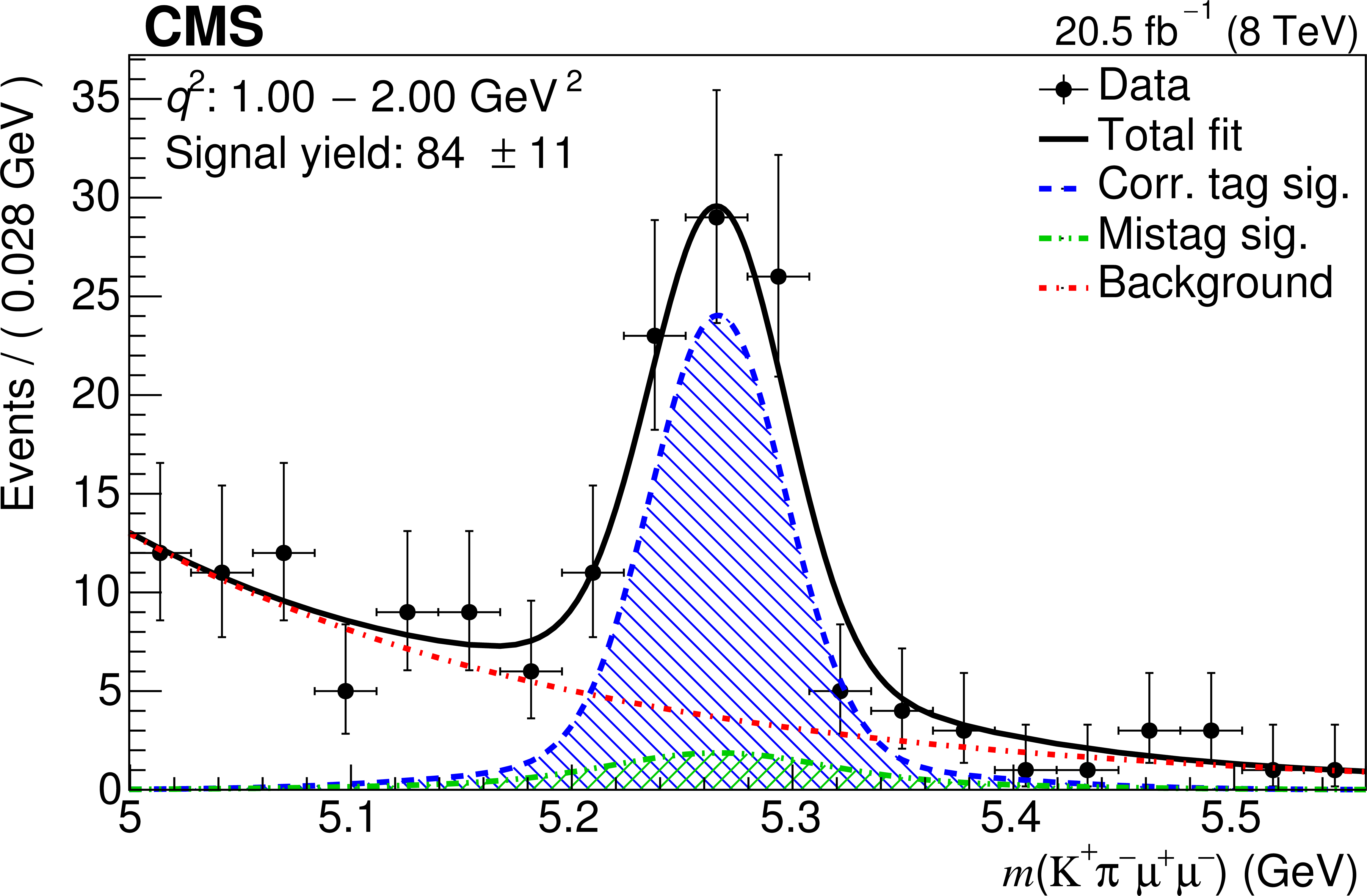
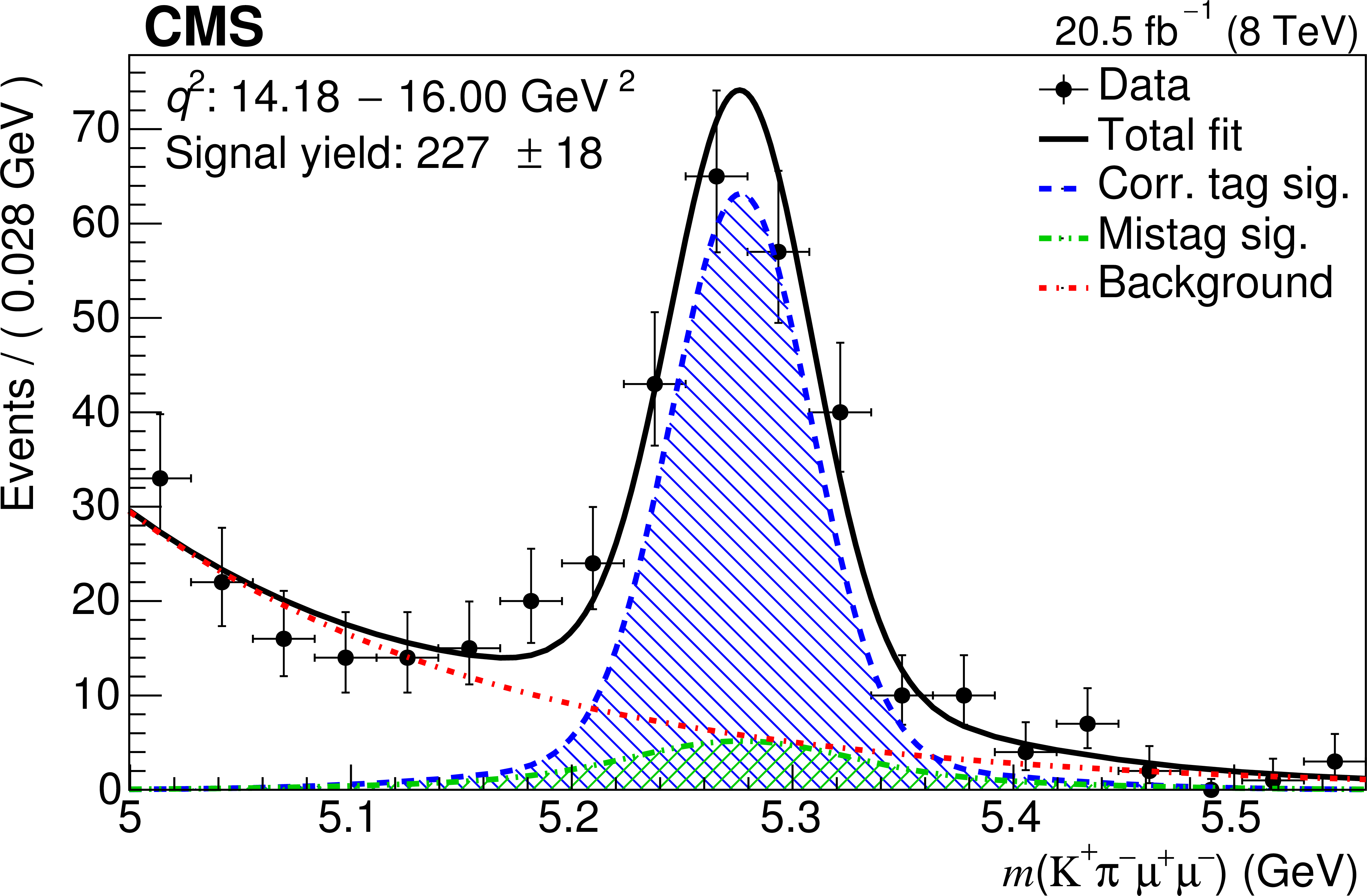
Figure 2-a:
The $ {\mathrm {K^+}} {\pi ^-} {{\mu ^+}} {{\mu ^-}}$ invariant mass distributions for the seven signal $q^2$ bins and the combined 1 $ < q^2 < $ 6 GeV$^2$ bin. Overlaid on each is the projection of the results for the total fit, as well as the three components: correctly tagged signal, mistagged signal, and background. The vertical bars give the statistical uncertainties, the horizontal bars the bin widths. |

png pdf |
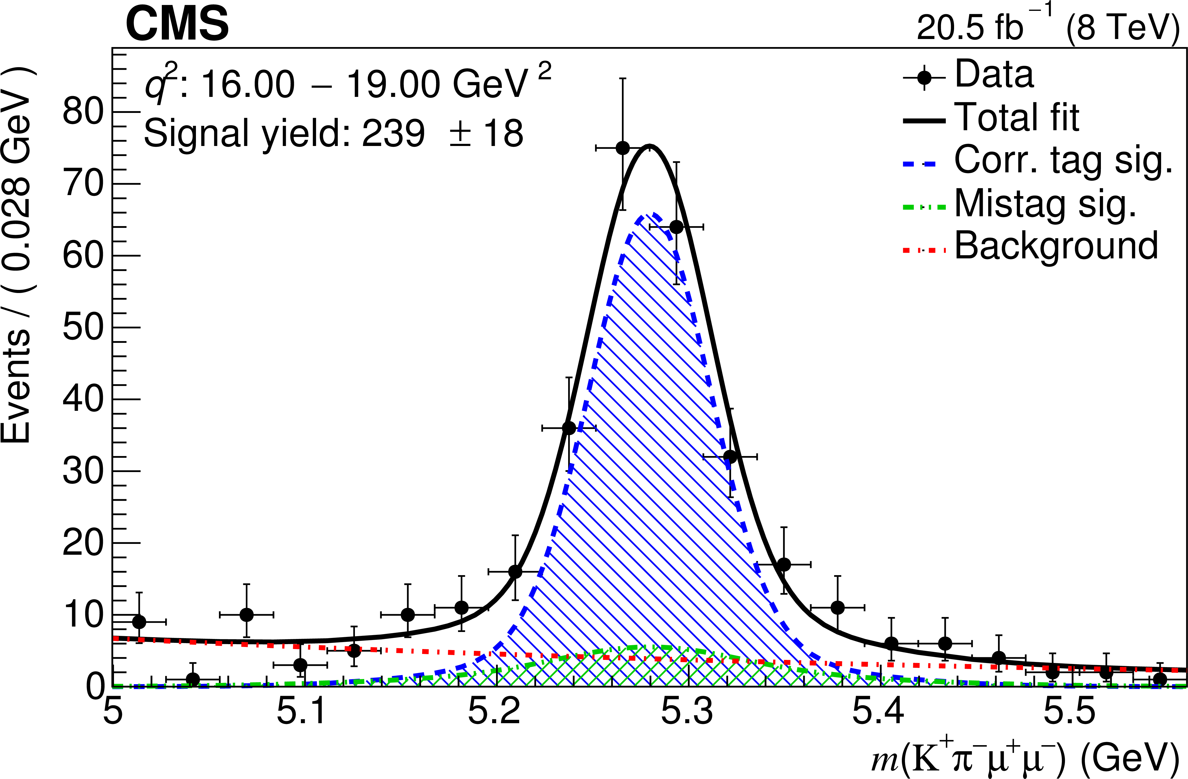
Figure 2-b:
The $ {\mathrm {K^+}} {\pi ^-} {{\mu ^+}} {{\mu ^-}}$ invariant mass distributions for the seven signal $q^2$ bins and the combined 1 $ < q^2 < $ 6 GeV$^2$ bin. Overlaid on each is the projection of the results for the total fit, as well as the three components: correctly tagged signal, mistagged signal, and background. The vertical bars give the statistical uncertainties, the horizontal bars the bin widths. |
png pdf |
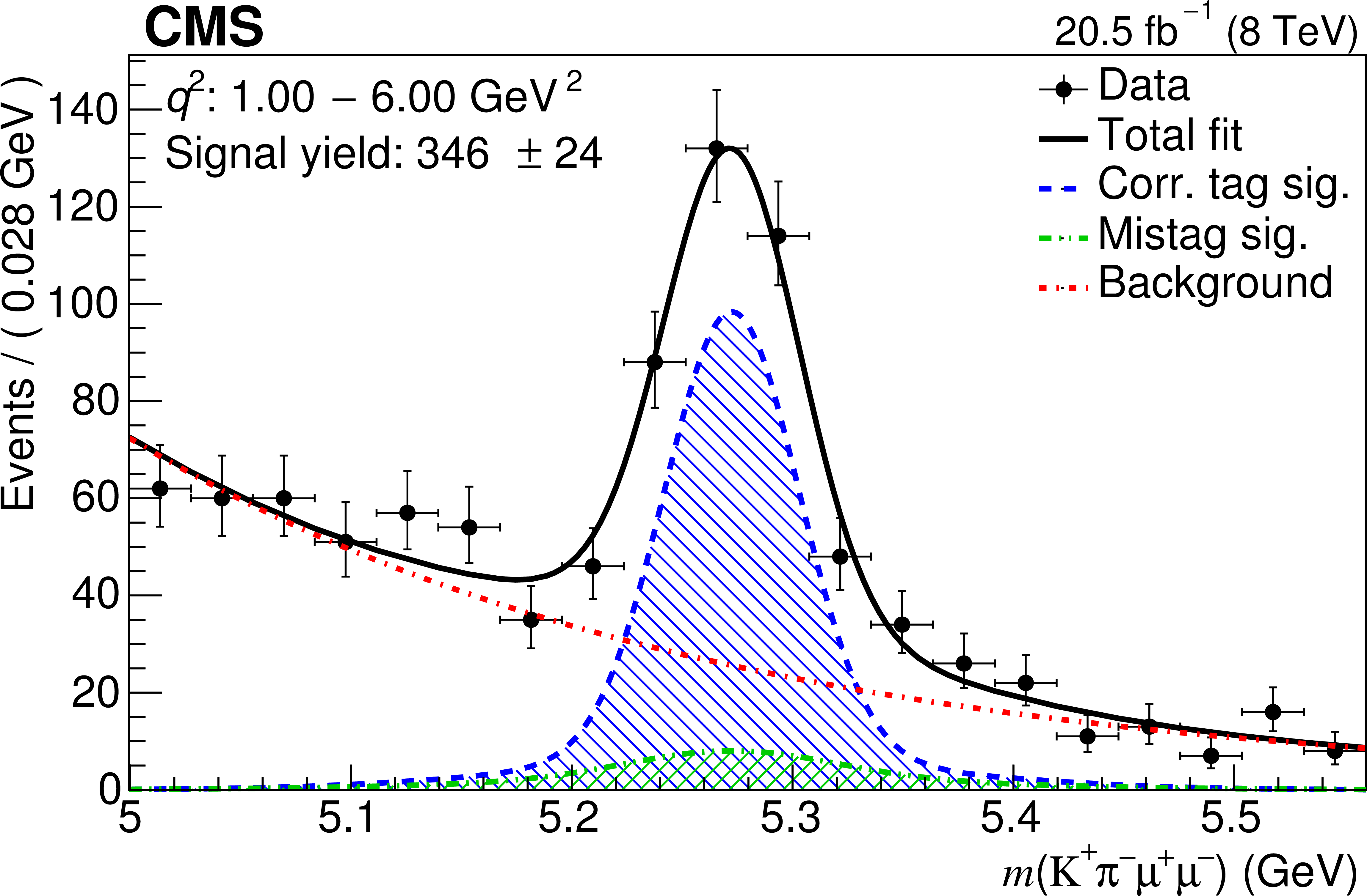
Figure 2-c:
The $ {\mathrm {K^+}} {\pi ^-} {{\mu ^+}} {{\mu ^-}}$ invariant mass distributions for the seven signal $q^2$ bins and the combined 1 $ < q^2 < $ 6 GeV$^2$ bin. Overlaid on each is the projection of the results for the total fit, as well as the three components: correctly tagged signal, mistagged signal, and background. The vertical bars give the statistical uncertainties, the horizontal bars the bin widths. |

png pdf |
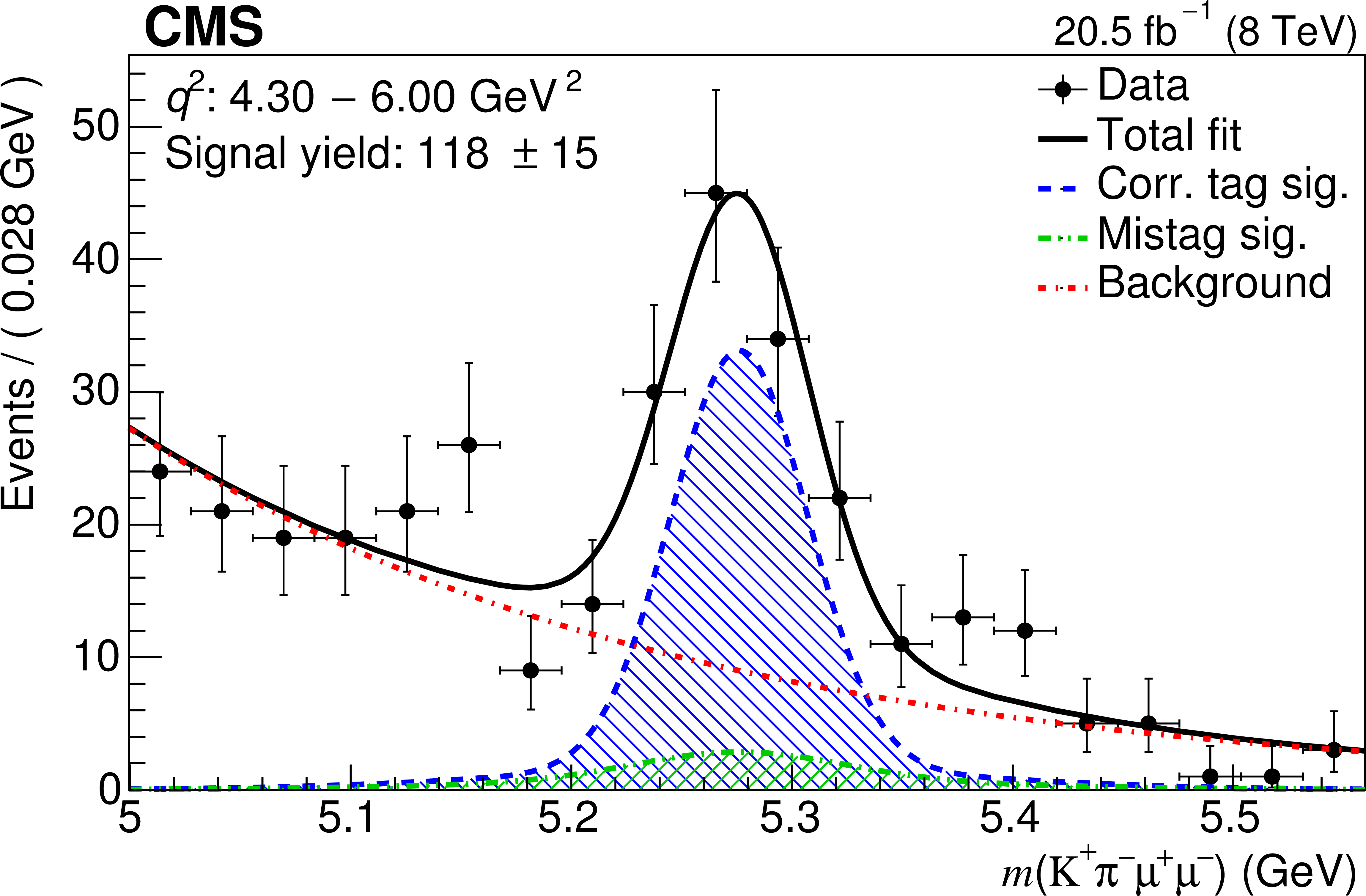
Figure 2-d:
The $ {\mathrm {K^+}} {\pi ^-} {{\mu ^+}} {{\mu ^-}}$ invariant mass distributions for the seven signal $q^2$ bins and the combined 1 $ < q^2 < $ 6 GeV$^2$ bin. Overlaid on each is the projection of the results for the total fit, as well as the three components: correctly tagged signal, mistagged signal, and background. The vertical bars give the statistical uncertainties, the horizontal bars the bin widths. |
png pdf |
Figure 2-e:
The $ {\mathrm {K^+}} {\pi ^-} {{\mu ^+}} {{\mu ^-}}$ invariant mass distributions for the seven signal $q^2$ bins and the combined 1 $ < q^2 < $ 6 GeV$^2$ bin. Overlaid on each is the projection of the results for the total fit, as well as the three components: correctly tagged signal, mistagged signal, and background. The vertical bars give the statistical uncertainties, the horizontal bars the bin widths. |
png pdf |
Figure 2-f:
The $ {\mathrm {K^+}} {\pi ^-} {{\mu ^+}} {{\mu ^-}}$ invariant mass distributions for the seven signal $q^2$ bins and the combined 1 $ < q^2 < $ 6 GeV$^2$ bin. Overlaid on each is the projection of the results for the total fit, as well as the three components: correctly tagged signal, mistagged signal, and background. The vertical bars give the statistical uncertainties, the horizontal bars the bin widths. |
png pdf |
Figure 2-g:
The $ {\mathrm {K^+}} {\pi ^-} {{\mu ^+}} {{\mu ^-}}$ invariant mass distributions for the seven signal $q^2$ bins and the combined 1 $ < q^2 < $ 6 GeV$^2$ bin. Overlaid on each is the projection of the results for the total fit, as well as the three components: correctly tagged signal, mistagged signal, and background. The vertical bars give the statistical uncertainties, the horizontal bars the bin widths. |
png pdf |
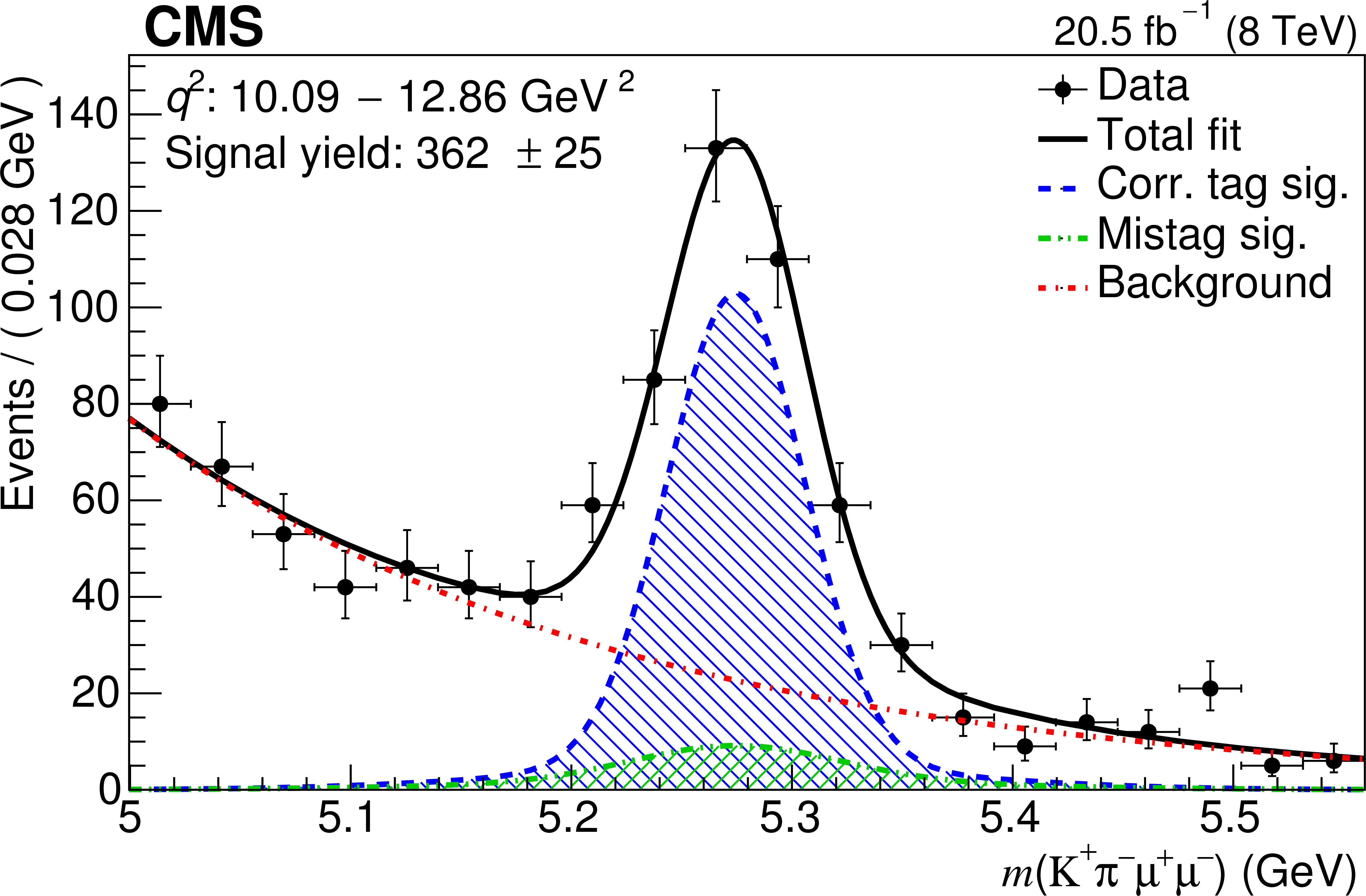
Figure 2-h:
The $ {\mathrm {K^+}} {\pi ^-} {{\mu ^+}} {{\mu ^-}}$ invariant mass distributions for the seven signal $q^2$ bins and the combined 1 $ < q^2 < $ 6 GeV$^2$ bin. Overlaid on each is the projection of the results for the total fit, as well as the three components: correctly tagged signal, mistagged signal, and background. The vertical bars give the statistical uncertainties, the horizontal bars the bin widths. |
png pdf |
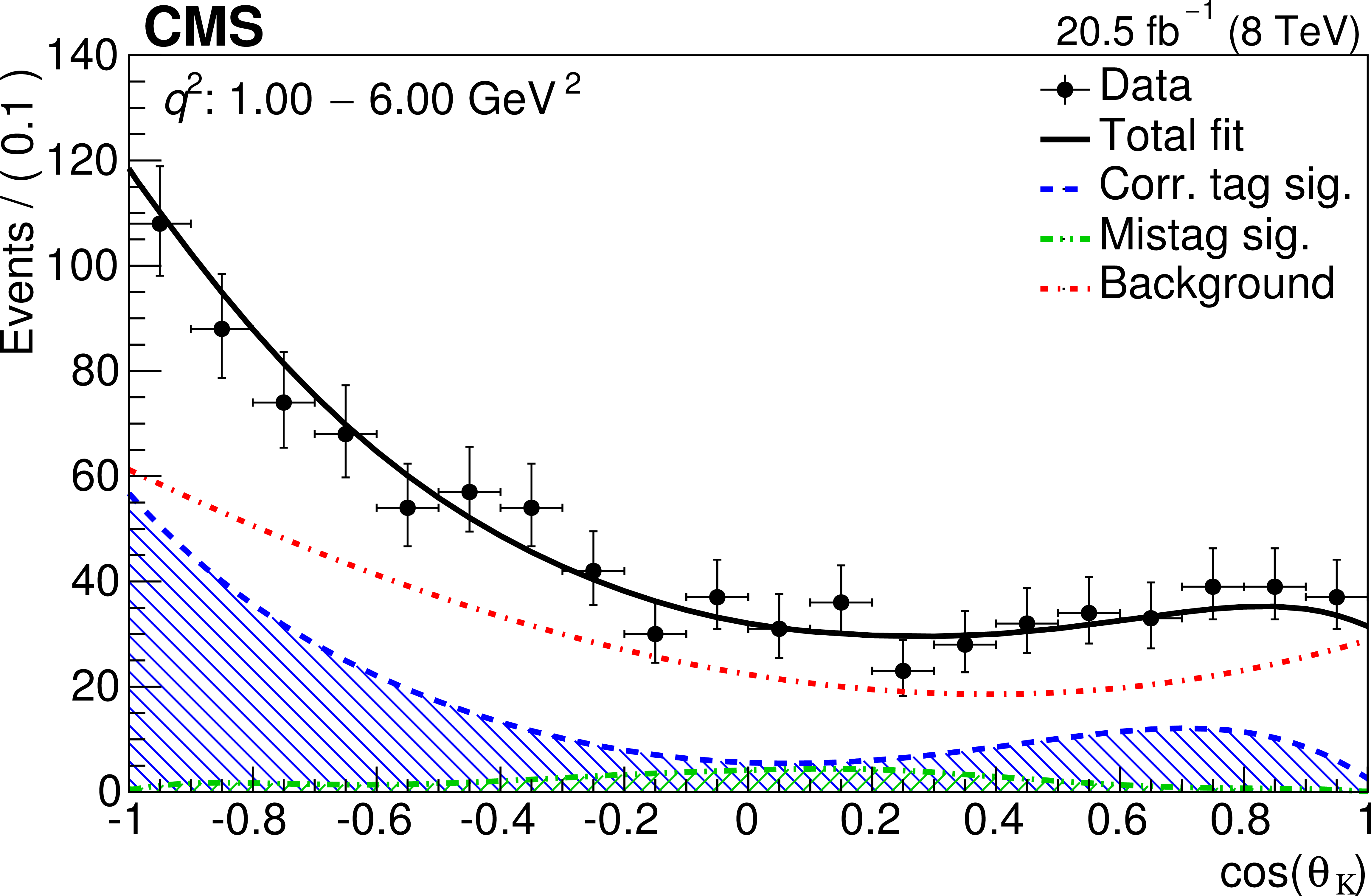
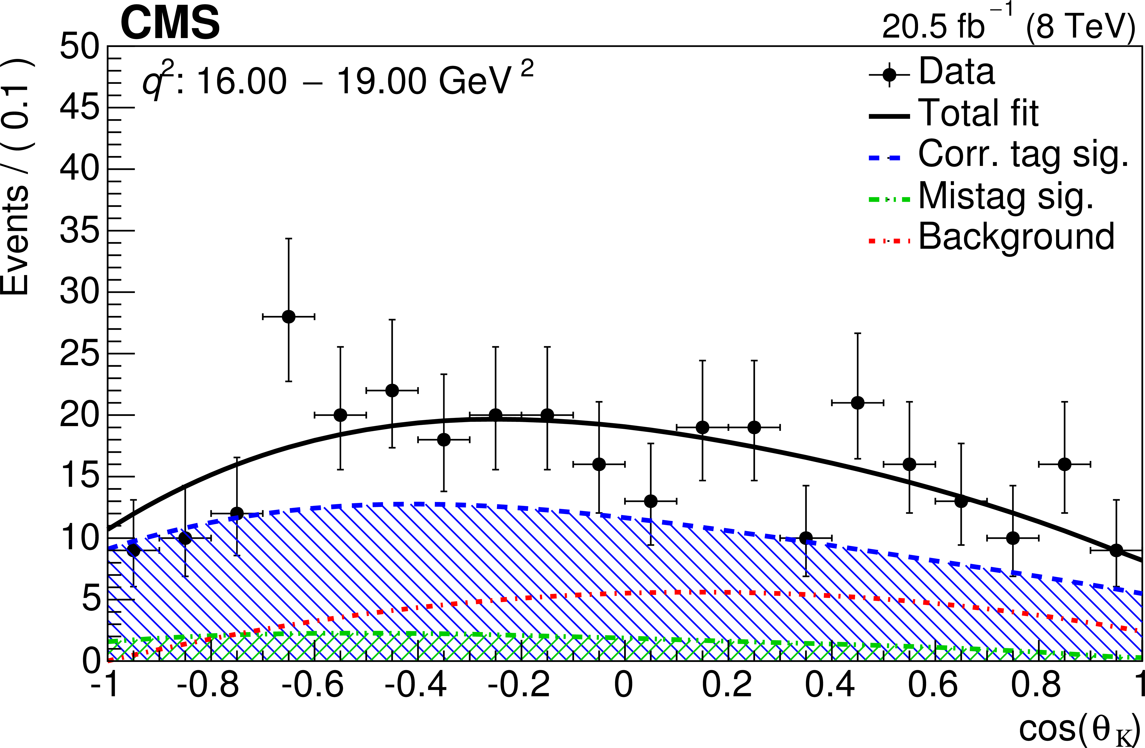
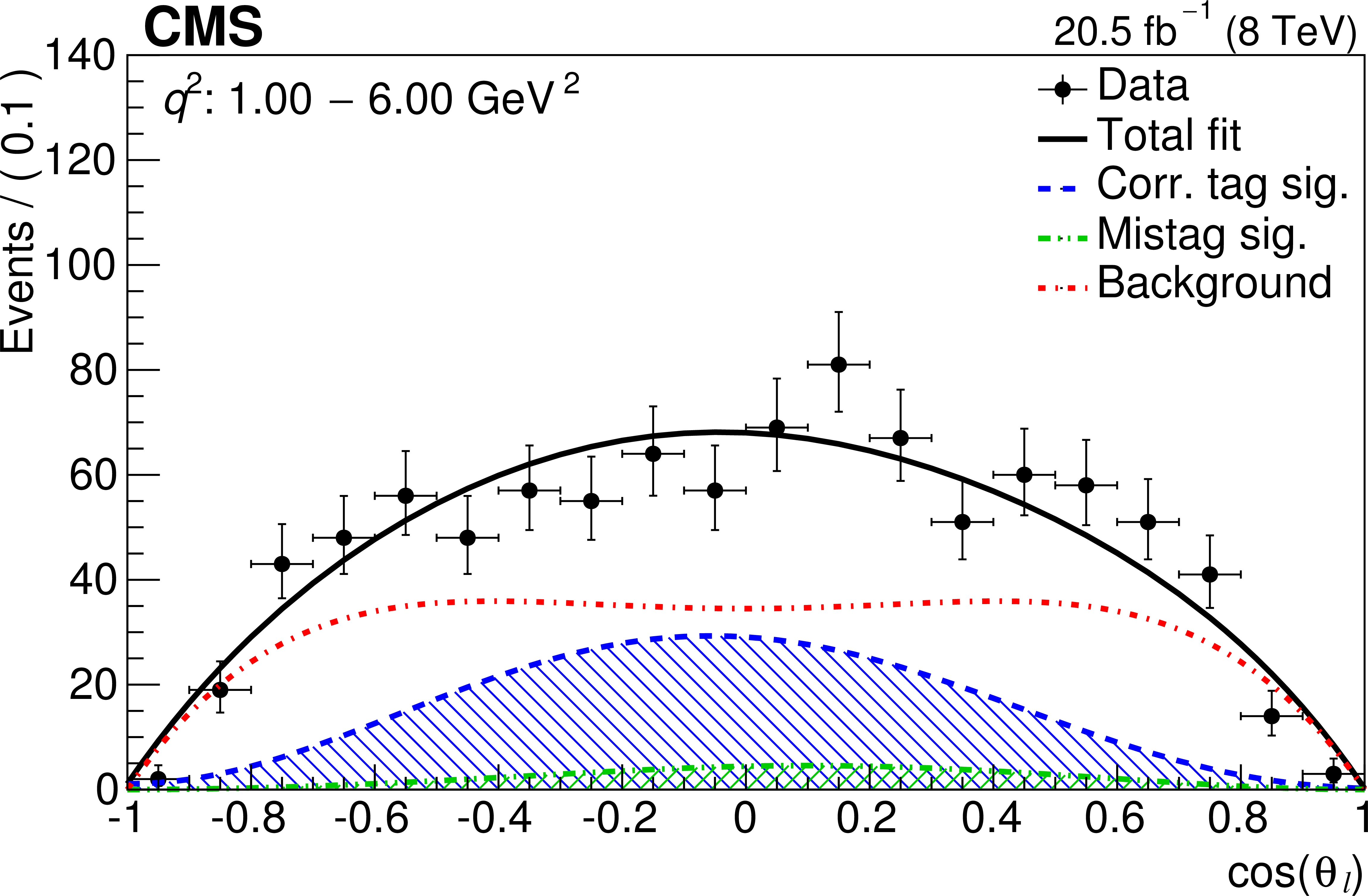
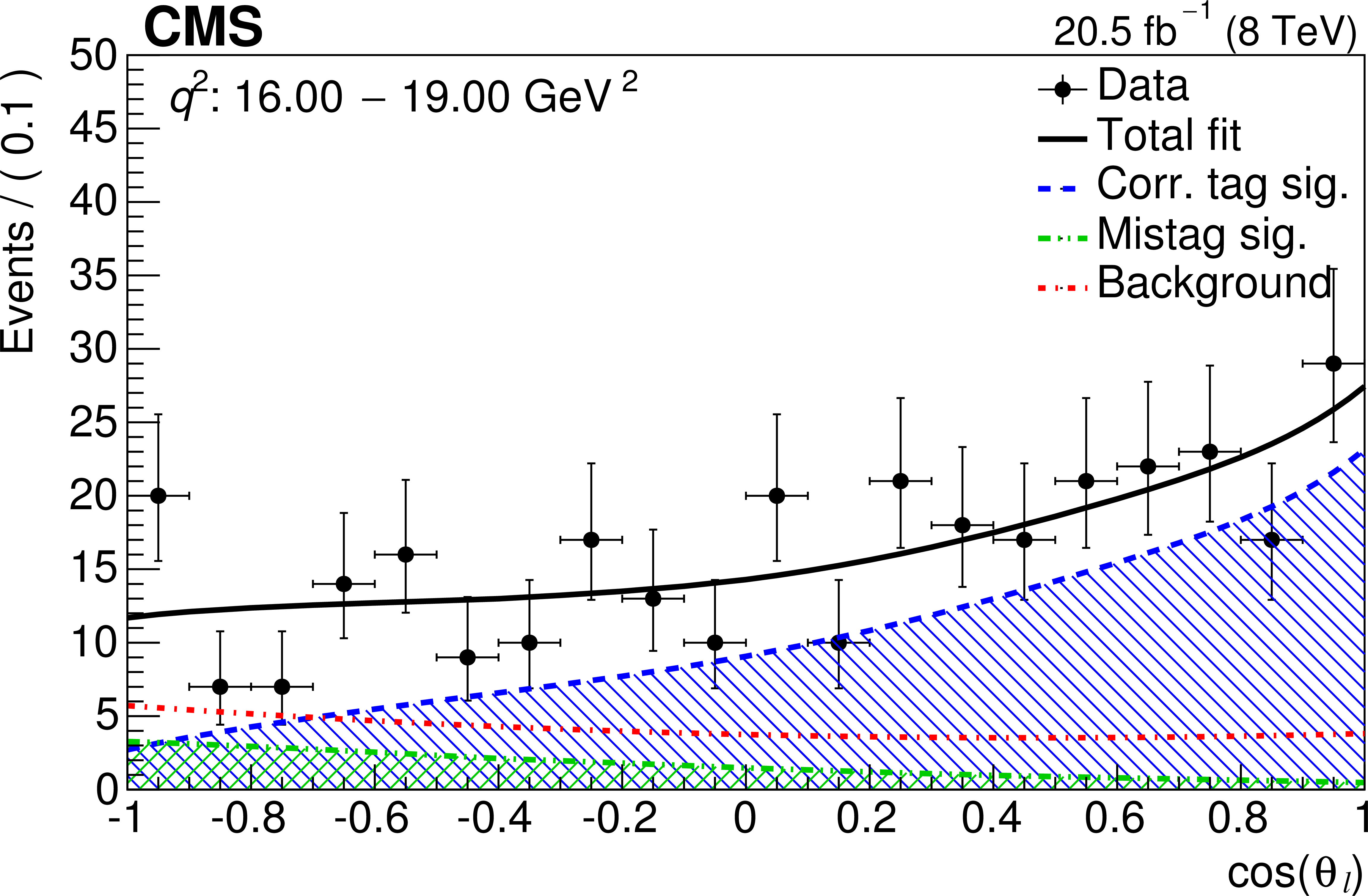
Figure 3-a:
Data and fit results for 1 $ < q^2 < $ 6 GeV$^2$ (a) and 16 $ < q^2 < $ 19 GeV$^2$ (b), projected onto the $\cos \theta _ {\mathrm {K}} $ axis (a), and $\cos \theta_l$ axis (b). The fit results show the total fit, as well as the three components: correctly tagged signal, mistagged signal, and background. The vertical bars give the statistical uncertainties, the horizontal bars the bin widths. |
png pdf |
Figure 3-b:
Data and fit results for 1 $ < q^2 < $ 6 GeV$^2$ (a) and 16 $ < q^2 < $ 19 GeV$^2$ (b), projected onto the $\cos \theta _ {\mathrm {K}} $ axis (a), and $\cos \theta_l$ axis (b). The fit results show the total fit, as well as the three components: correctly tagged signal, mistagged signal, and background. The vertical bars give the statistical uncertainties, the horizontal bars the bin widths. |
png pdf |
Figure 3-c:
Data and fit results for 1 $ < q^2 < $ 6 GeV$^2$ (a) and 16 $ < q^2 < $ 19 GeV$^2$ (b), projected onto the $\cos \theta _ {\mathrm {K}} $ axis (a), and $\cos \theta_l$ axis (b). The fit results show the total fit, as well as the three components: correctly tagged signal, mistagged signal, and background. The vertical bars give the statistical uncertainties, the horizontal bars the bin widths. |
png pdf |
Figure 3-d:
Data and fit results for 1 $ < q^2 < $ 6 GeV$^2$ (a) and 16 $ < q^2 < $ 19 GeV$^2$ (b), projected onto the $\cos \theta _ {\mathrm {K}} $ axis (a), and $\cos \theta_l$ axis (b). The fit results show the total fit, as well as the three components: correctly tagged signal, mistagged signal, and background. The vertical bars give the statistical uncertainties, the horizontal bars the bin widths. |
png pdf |
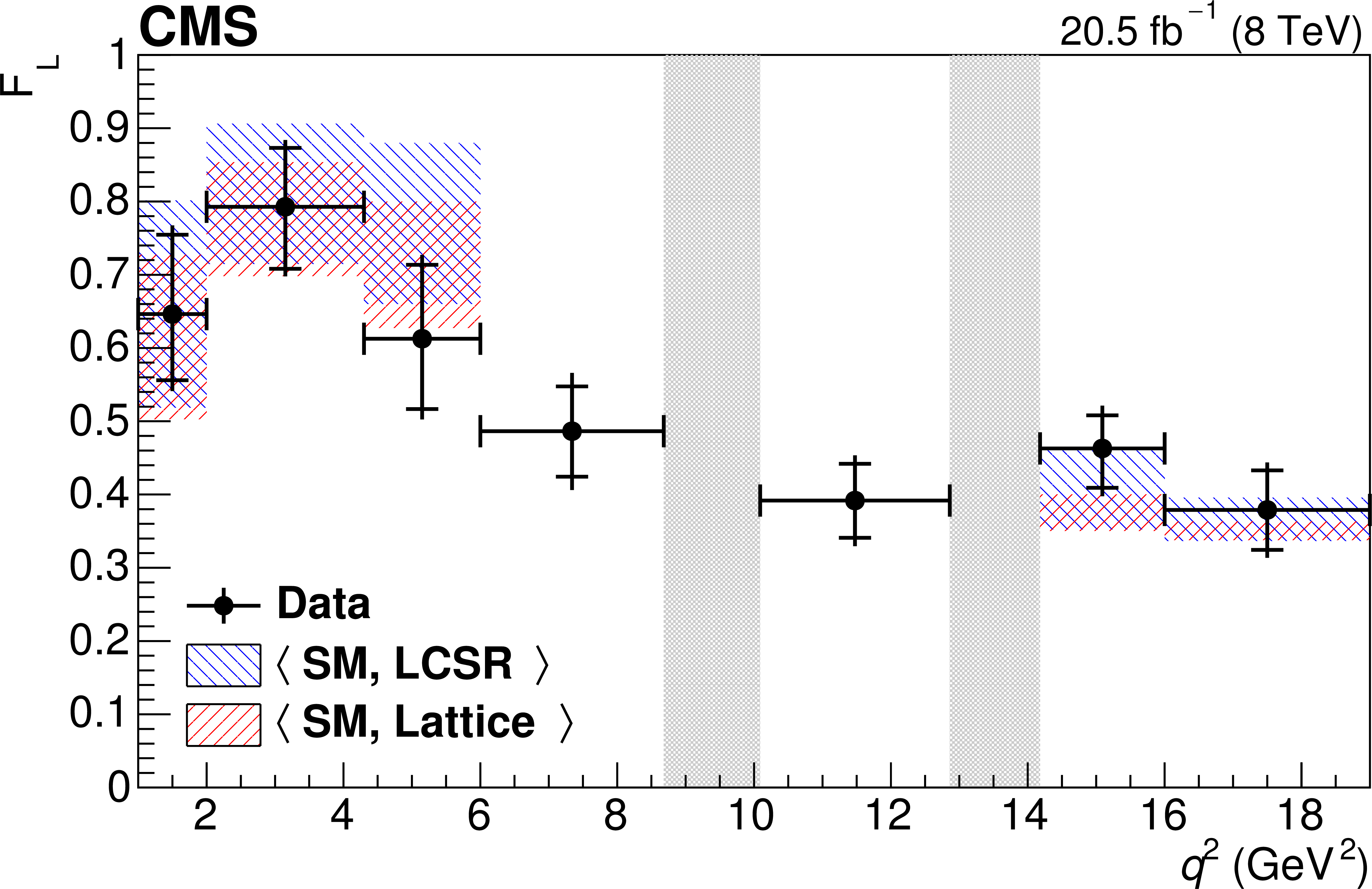
Figure 4-a:
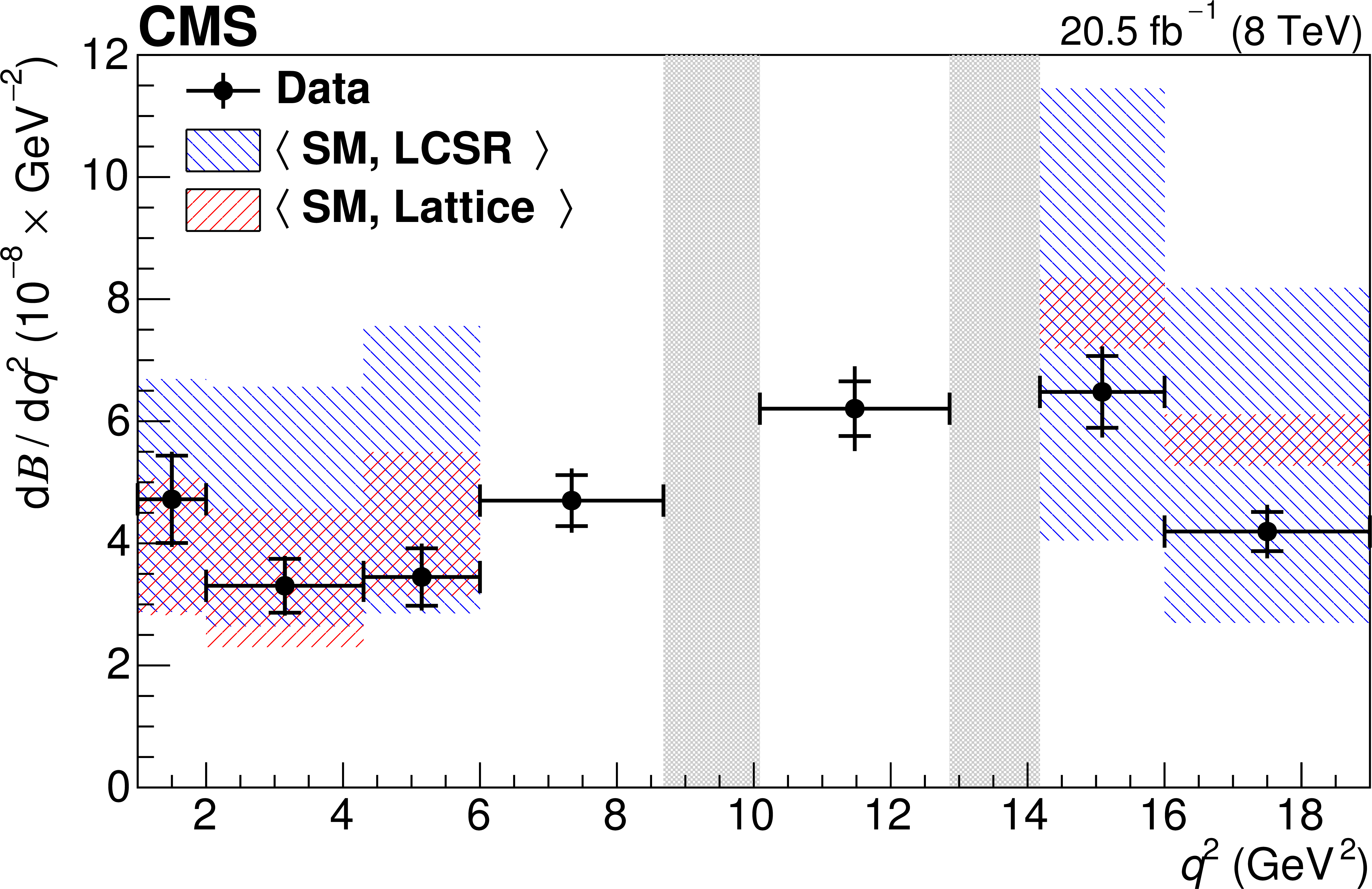
Measured values of $F_\mathrm {L}$, $A_\mathrm {FB}$, and $ {\mathrm {d}}{}\mathcal {B}/ {\mathrm {d}}{}q^2$ versus $q^2$ for $ { {{\mathrm {B}^0}}\to {\mathrm {K}^{\ast 0}} {{\mu ^+}} {{\mu ^-}}} $. The statistical uncertainty is shown by the inner vertical bars, while the outer vertical bars give the total uncertainty. The horizontal bars show the bin widths. The vertical shaded regions correspond to the $ {\mathrm {J} / \psi }$ and $\psi^{\prime}$ resonances. The other shaded regions show the two SM predictions after rate averaging across the $q^2$ bins to provide a direct comparison to the data. Controlled theoretical predictions are not available near the $ {\mathrm {J}/\psi }$ and $\psi^{\prime}$ resonances. |

png pdf |
Figure 4-b:
Measured values of $F_\mathrm {L}$, $A_\mathrm {FB}$, and $ {\mathrm {d}}{}\mathcal {B}/ {\mathrm {d}}{}q^2$ versus $q^2$ for $ { {{\mathrm {B}^0}}\to {\mathrm {K}^{\ast 0}} {{\mu ^+}} {{\mu ^-}}} $. The statistical uncertainty is shown by the inner vertical bars, while the outer vertical bars give the total uncertainty. The horizontal bars show the bin widths. The vertical shaded regions correspond to the $ {\mathrm {J} / \psi }$ and $\psi^{\prime}$ resonances. The other shaded regions show the two SM predictions after rate averaging across the $q^2$ bins to provide a direct comparison to the data. Controlled theoretical predictions are not available near the $ {\mathrm {J}/\psi }$ and $\psi^{\prime}$ resonances. |
png pdf |
Figure 4-c:
Measured values of $F_\mathrm {L}$, $A_\mathrm {FB}$, and $ {\mathrm {d}}{}\mathcal {B}/ {\mathrm {d}}{}q^2$ versus $q^2$ for $ { {{\mathrm {B}^0}}\to {\mathrm {K}^{\ast 0}} {{\mu ^+}} {{\mu ^-}}} $. The statistical uncertainty is shown by the inner vertical bars, while the outer vertical bars give the total uncertainty. The horizontal bars show the bin widths. The vertical shaded regions correspond to the $ {\mathrm {J} / \psi }$ and $\psi^{\prime}$ resonances. The other shaded regions show the two SM predictions after rate averaging across the $q^2$ bins to provide a direct comparison to the data. Controlled theoretical predictions are not available near the $ {\mathrm {J}/\psi }$ and $\psi^{\prime}$ resonances. |

png pdf |
Figure 5-a:
Measured values of $F_\mathrm {L}$, $A_\mathrm {FB}$, and $ {\mathrm {d}}{}\mathcal {B}/ {\mathrm {d}}{}q^2$ versus $q^2$ for $ { {{\mathrm {B}^0}}\to {\mathrm {K}^{\ast 0}} {{\mu ^+}} {{\mu ^-}}} $ from CMS (combination of the 7 TeV results and this analysis), Belle, CDF, BaBar, and LHCb. The CMS and LHCb results are from $ { {{\mathrm {B}^0}}\to {\mathrm {K}^{\ast 0}} {{\mu ^+}} {{\mu ^-}}} $ decays. The remaining experiments add the corresponding $ {{\mathrm {B}^{+}}}$ decay, and the BaBar and Belle experiments also include the dielectron mode. The vertical bars give the total uncertainty. The horizontal bars show the bin widths. The horizontal positions of the data points are staggered to improve legibility. The vertical shaded regions correspond to the $ {\mathrm {J}/\psi }$ and $\psi^{\prime}$ resonances. |

png pdf |
Figure 5-b:
Measured values of $F_\mathrm {L}$, $A_\mathrm {FB}$, and $ {\mathrm {d}}{}\mathcal {B}/ {\mathrm {d}}{}q^2$ versus $q^2$ for $ { {{\mathrm {B}^0}}\to {\mathrm {K}^{\ast 0}} {{\mu ^+}} {{\mu ^-}}} $ from CMS (combination of the 7 TeV results and this analysis), Belle, CDF, BaBar, and LHCb. The CMS and LHCb results are from $ { {{\mathrm {B}^0}}\to {\mathrm {K}^{\ast 0}} {{\mu ^+}} {{\mu ^-}}} $ decays. The remaining experiments add the corresponding $ {{\mathrm {B}^{+}}}$ decay, and the BaBar and Belle experiments also include the dielectron mode. The vertical bars give the total uncertainty. The horizontal bars show the bin widths. The horizontal positions of the data points are staggered to improve legibility. The vertical shaded regions correspond to the $ {\mathrm {J}/\psi }$ and $\psi^{\prime}$ resonances. |

png pdf |
Figure 5-c:
Measured values of $F_\mathrm {L}$, $A_\mathrm {FB}$, and $ {\mathrm {d}}{}\mathcal {B}/ {\mathrm {d}}{}q^2$ versus $q^2$ for $ { {{\mathrm {B}^0}}\to {\mathrm {K}^{\ast 0}} {{\mu ^+}} {{\mu ^-}}} $ from CMS (combination of the 7 TeV results and this analysis), Belle, CDF, BaBar, and LHCb. The CMS and LHCb results are from $ { {{\mathrm {B}^0}}\to {\mathrm {K}^{\ast 0}} {{\mu ^+}} {{\mu ^-}}} $ decays. The remaining experiments add the corresponding $ {{\mathrm {B}^{+}}}$ decay, and the BaBar and Belle experiments also include the dielectron mode. The vertical bars give the total uncertainty. The horizontal bars show the bin widths. The horizontal positions of the data points are staggered to improve legibility. The vertical shaded regions correspond to the $ {\mathrm {J}/\psi }$ and $\psi^{\prime}$ resonances. |
| Tables | |
png pdf |
Table 1:
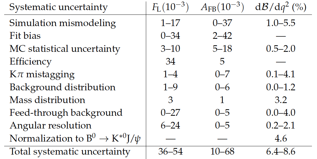
Systematic uncertainty contributions for the measurements of $F_\mathrm {L}$, $A_\mathrm {FB}$, and the branching fraction for the decay $ { {{\mathrm {B}^0}}\to {\mathrm {K}^{\ast 0}} {{\mu ^+}} {{\mu ^-}}} $. The values for $F_\mathrm {L}$ and $A_\mathrm {FB}$ are absolute, while the values for the branching fraction are relative. The total uncertainty in each $q^2$ bin is obtained by adding each contribution in quadrature. For each item, the range indicates the variation of the uncertainty in the signal $q^2$ bins. |

png pdf |
Table 2:
The measured values of signal yield (including both correctly tagged and mistagged events), $F_\mathrm {L}$, $A_\mathrm {FB}$, and differential branching fraction for the decay $ { {{\mathrm {B}^0}}\to {\mathrm {K}^{\ast 0}} {{\mu ^+}} {{\mu ^-}}} $ in bins of $q^2$. The first uncertainty is statistical and the second (when present) is systematic. The bin ranges are selected to allow comparisons to previous measurements. |
png pdf |
Table 3:
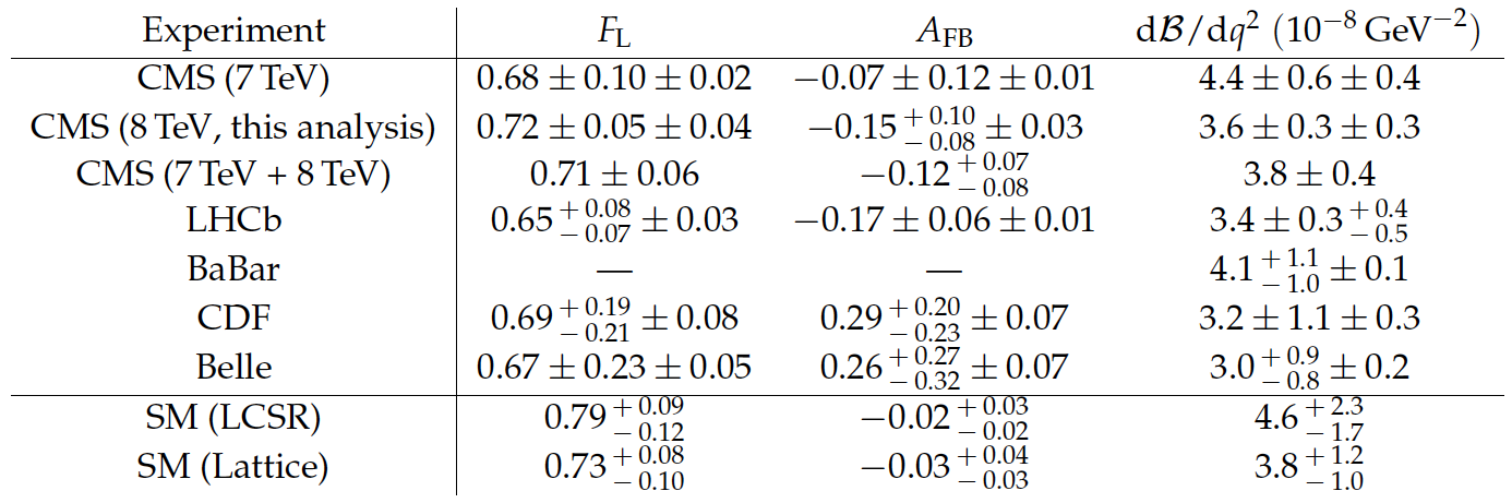
Measurements from CMS (the 7 TeV results, this work for 8 TeV, and the combination), LHCb, BaBar, CDF, and Belle of $F_\mathrm {L}$, $A_\mathrm {FB}$, and $ {\mathrm {d}}{}\mathcal {B}/ {\mathrm {d}}{}q^2$ in the region 1 $ < q^2 < $ 6 GeV$^2$ for the decay $ { {{\mathrm {B}^0}}\to {\mathrm {K}^{\ast 0}} {{\mu ^+}} {{\mu ^-}}} $. The CMS and LHCb results are from $ { {{\mathrm {B}^0}}\to {\mathrm {K}^{\ast 0}} {{\mu ^+}} {{\mu ^-}}} $ decays. The remaining experiments add the corresponding $ {{\mathrm {B}^{+}}}$ decay, and the BaBar and Belle experiments also include the dielectron mode. The first uncertainty is statistical and the second is systematic. For the combined CMS results, only the total uncertainty is reported. The two SM predictions are also given. |
| Summary |
| Using pp collision data recorded at $\sqrt{s} =$ 8 TeV with the CMS detector at the LHC, corresponding to an integrated luminosity 20.5 fb$^{-1}$, an angular analysis has been carried out on the decay $ \mathrm{ B^0 \to K^{*0} \mu^{+} \mu^{-} } $. The data used for this analysis include 1430 signal decays. For each bin of the dimuon invariant mass squared ($q^2$), unbinned maximum-likelihood fits were performed to the distributions of the $ \mathrm{ K^+ \pi^- \mu^+ \mu^- } $ invariant mass and two decay angles, to obtain values of the forward-backward asymmetry of the muons, $A_{\mathrm{FB}}$ , the fraction of longitudinal polarization of the $\mathrm{ K^{*0} }$, $F_{\mathrm{L}}$, and the differential branching fraction, $ \mathrm{d} \mathcal{B}/ \mathrm{d} q^2$. The results are among the most precise to date and are consistent with standard model predictions and previous measurements. |
|
|
Compact Muon Solenoid LHC, CERN |
|

|

|

|

|

|