

Compact Muon Solenoid
LHC, CERN
| CMS-EWK-11-016 ; CERN-PH-EP-2015-031 | ||
| A study of final-state radiation in decays of Z bosons produced in pp collisions at 7 TeV | ||
| CMS Collaboration | ||
| 27 February 2015 | ||
| Phys. Rev. D 91 (2015) 092012 | ||
| Abstract: The differential cross sections for the production of photons in Z to $ \mu^+ \mu^- \gamma $ decays are presented as a function of the transverse energy of the photon and its separation from the nearest muon. The data for these measurements were collected with the CMS detector and correspond to an integrated luminosity of 4.7 fb$ ^{-1} $ of pp collisions at $ \sqrt{s} $ = 7 TeV delivered by the CERN LHC. The cross sections are compared to simulations with POWHEG and PYTHIA, where PYTHIA is used to simulate parton showers and final-state photons. These simulations match the data to better than 5%. | ||
| Links: e-print arXiv:1502.07940 [hep-ex] (PDF) ; CDS record ; inSPIRE record ; Public twiki page ; Rivet record ; HepData record ; CADI line (restricted) ; | ||
| Figures | |
png pdf |
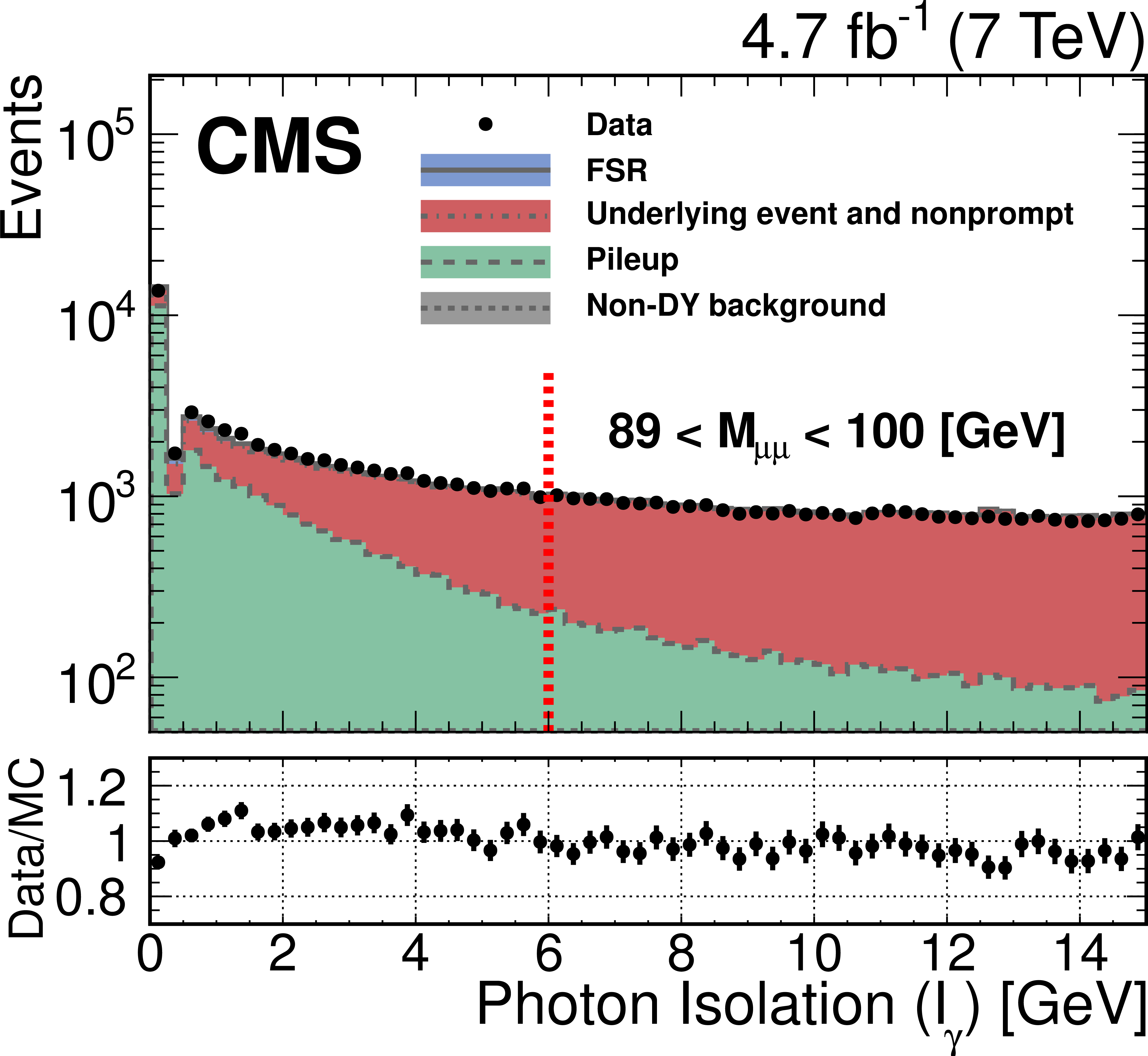
Figure 1-a:
Distributions of the photon isolation variable $I_{\gamma}$ for the control region (a) and for the signal region (b) after all corrections have been applied. The bottom panels display the ratio of data to the MC expectation. The requirement for FSR photons is $I_{\gamma} <$ 6 GeV. |
png pdf |
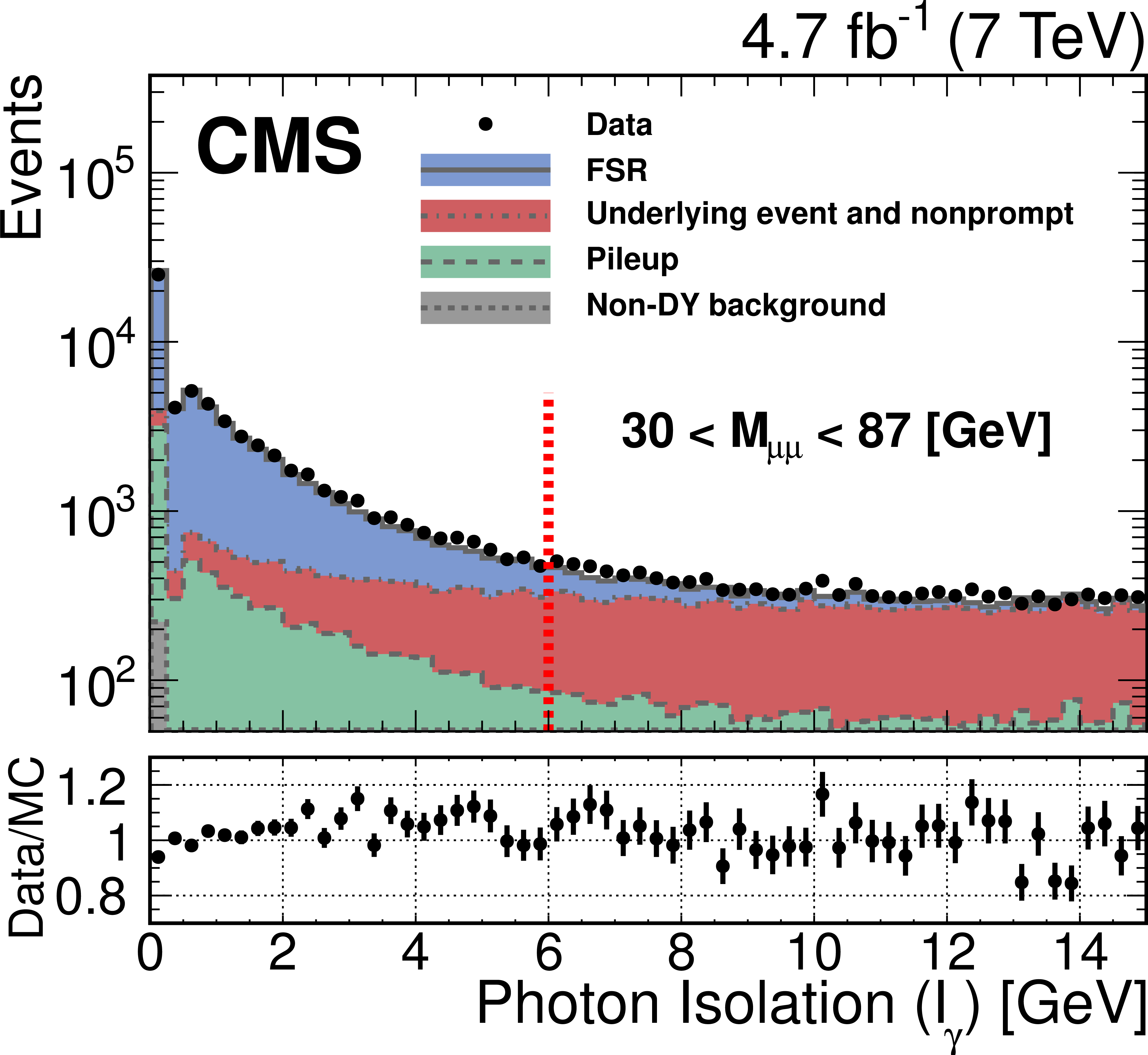
Figure 1-b:
Distributions of the photon isolation variable $I_{\gamma}$ for the control region (a) and for the signal region (b) after all corrections have been applied. The bottom panels display the ratio of data to the MC expectation. The requirement for FSR photons is $I_{\gamma} <$ 6 GeV. |
png pdf |
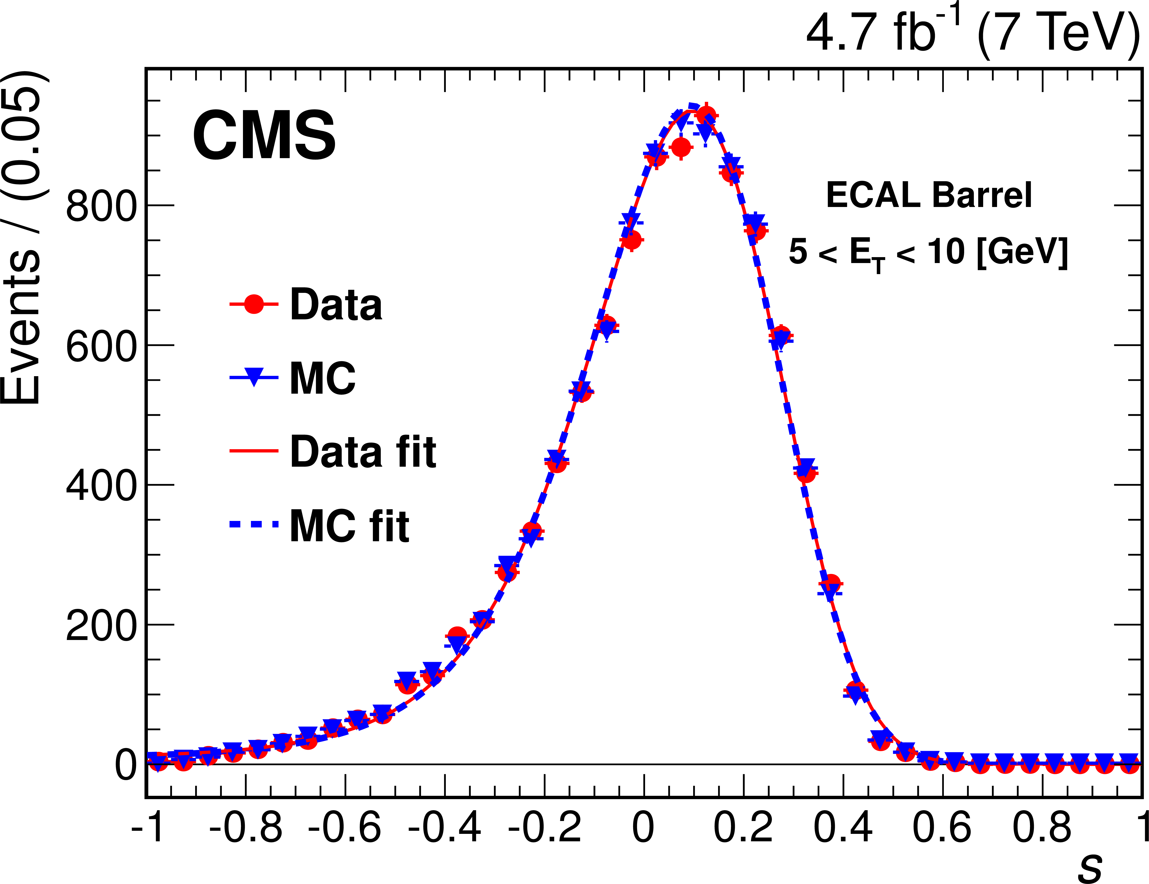
Figure 2-a:
Two examples of an $s$ distribution $s = 1-(M^2_{\mu\mu\gamma} -M^2_{\mu\mu})/(M^2_{\mathrm{Z}} - M^2_{\mu\mu})$ fit with a skewed Gaussian as described in the text. The (a) and (b) plots pertain to photons in the ECAL barrel with 5 $< E_{\mathrm{T}} <$ 10 GeV and in the ECAL endcaps with 20 $< E_{\mathrm{T}} <$ 40 GeV, respectively. The circle points and solid curve represent the data and the triangle points and dotted curve represent the simulation. |

png pdf |
Figure 2-b:
Two examples of an $s$ distribution $s = 1-(M^2_{\mu\mu\gamma} -M^2_{\mu\mu})/(M^2_{\mathrm{Z}} - M^2_{\mu\mu})$ fit with a skewed Gaussian as described in the text. The (a) and (b) plots pertain to photons in the ECAL barrel with 5 $< E_{\mathrm{T}} <$ 10 GeV and in the ECAL endcaps with 20 $< E_{\mathrm{T}} <$ 40 GeV, respectively. The circle points and solid curve represent the data and the triangle points and dotted curve represent the simulation. |
png pdf |
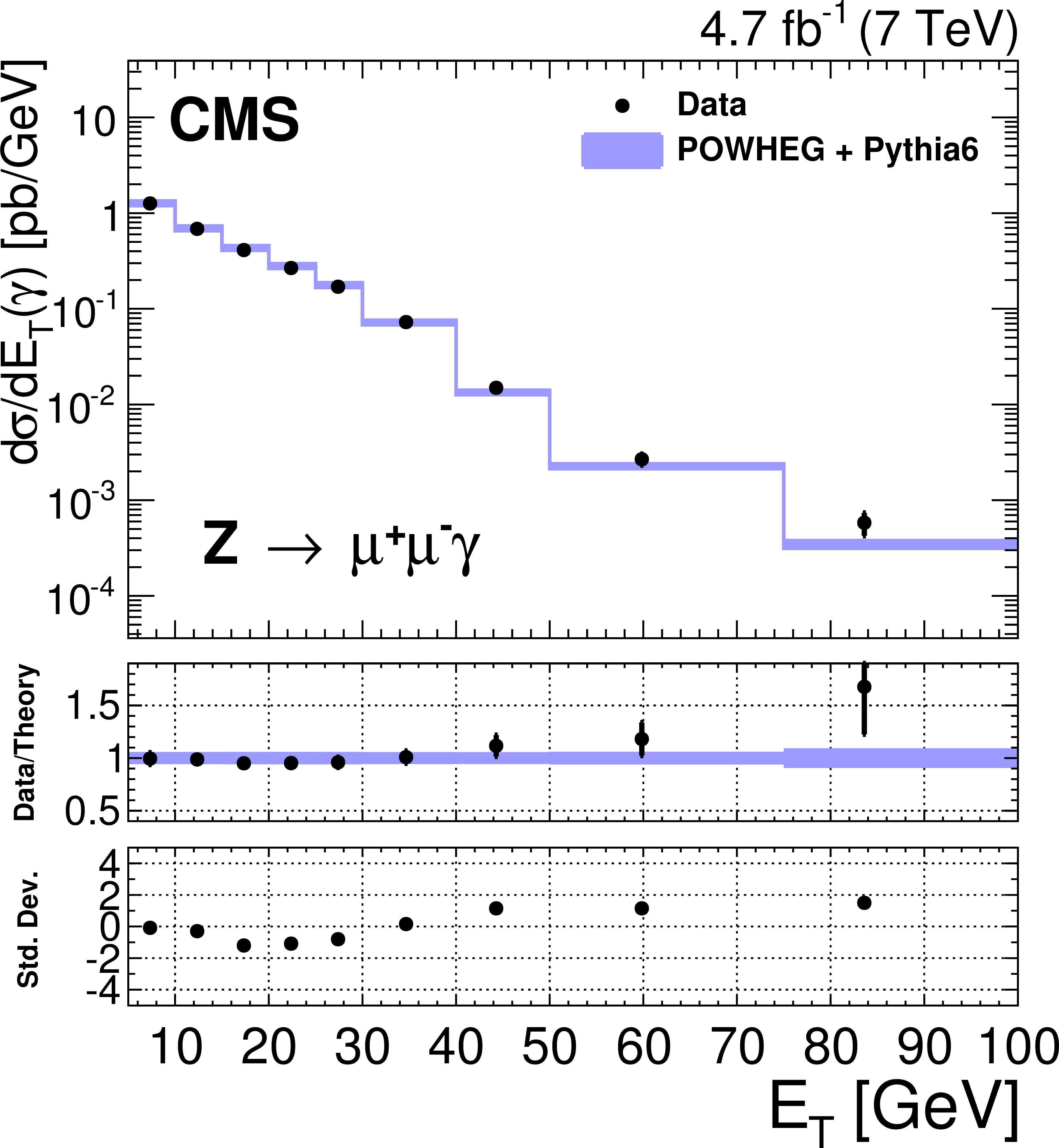
Figure 3-a:
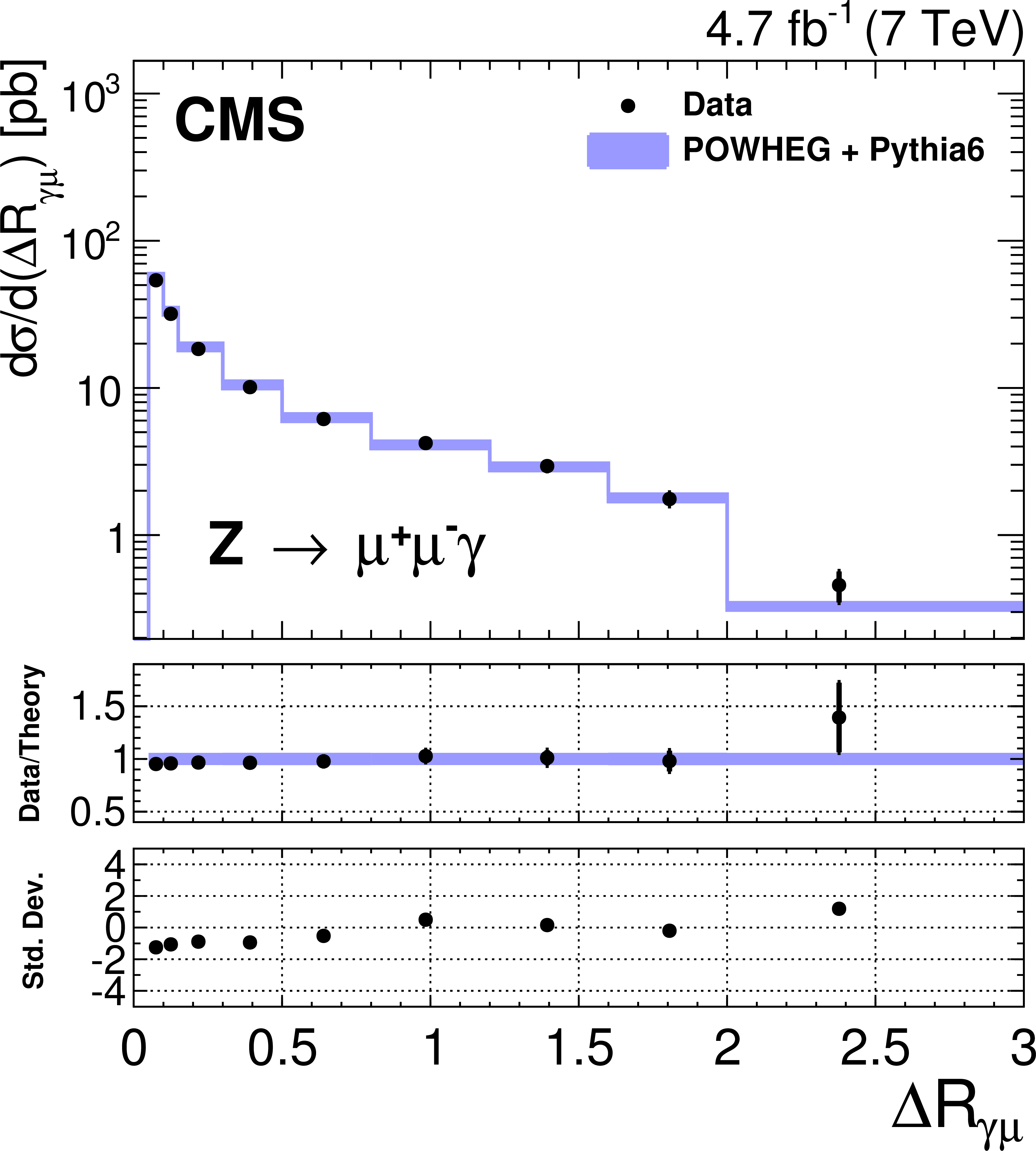
Measured differential cross sections $\mathrm{d}\sigma / \mathrm{d} E_{\mathrm{T}} $ (a) and $\mathrm{d}\sigma / \mathrm{d} \Delta R_{\mu\gamma}$ (b). The dots with error bars represent the data, and the shaded bands represent the POWHEG+PYTHIA calculation including theoretical uncertainties. The bottom panels display the ratio of data to the MC expectation. A bin-centering procedure has been applied. |
png pdf |
Figure 3-b:
Measured differential cross sections $\mathrm{d}\sigma / \mathrm{d} E_{\mathrm{T}} $ (a) and $\mathrm{d}\sigma / \mathrm{d} \Delta R_{\mu\gamma}$ (b). The dots with error bars represent the data, and the shaded bands represent the POWHEG+PYTHIA calculation including theoretical uncertainties. The bottom panels display the ratio of data to the MC expectation. A bin-centering procedure has been applied. |
png pdf |
Figure 4-a:
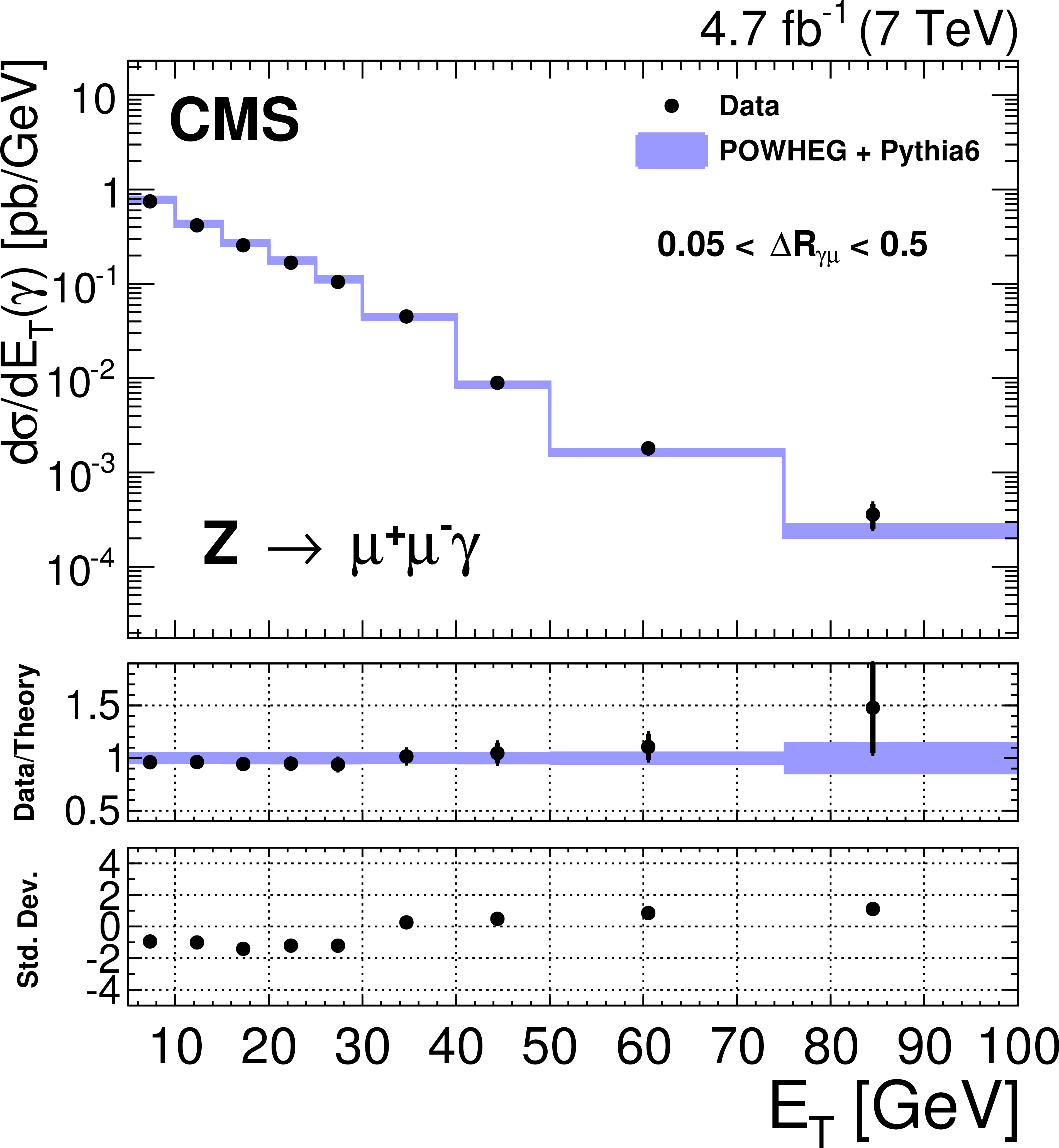
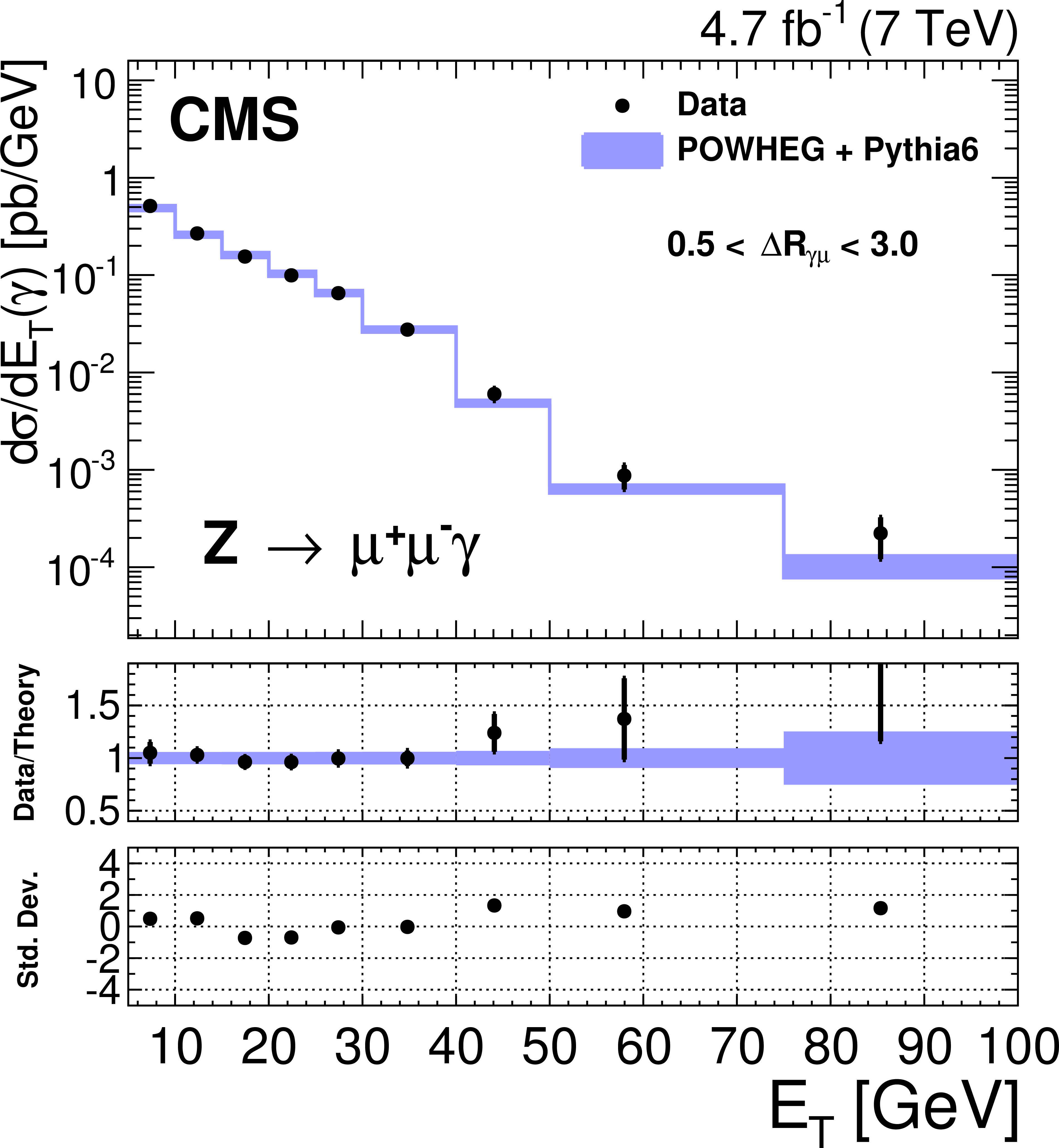
Measured differential cross sections $\mathrm{d}\sigma / \mathrm{d} E_{\mathrm{T}} $ for photons close to the muon (0.05 $< \mathrm{d}\sigma / \mathrm{d} \Delta R_{\mu\gamma}\le$ 0.5, a) and far from the muon (0.5 $< \mathrm{d}\sigma / \mathrm{d} \Delta R_{\mu\gamma} \le $ 3, b). The dots with error bars represent the data, and the shaded bands represent the POWHEG+PYTHIA calculation including theoretical uncertainties. The bottom panels display the ratio of data to the MC expectation. A bin-centering procedure has been applied. |
png pdf |
Figure 4-b:
Measured differential cross sections $\mathrm{d}\sigma / \mathrm{d} E_{\mathrm{T}} $ for photons close to the muon (0.05 $< \mathrm{d}\sigma / \mathrm{d} \Delta R_{\mu\gamma}\le$ 0.5, a) and far from the muon (0.5 $< \mathrm{d}\sigma / \mathrm{d} \Delta R_{\mu\gamma} \le $ 3, b). The dots with error bars represent the data, and the shaded bands represent the POWHEG+PYTHIA calculation including theoretical uncertainties. The bottom panels display the ratio of data to the MC expectation. A bin-centering procedure has been applied. |
png pdf |
Figure 5-a:
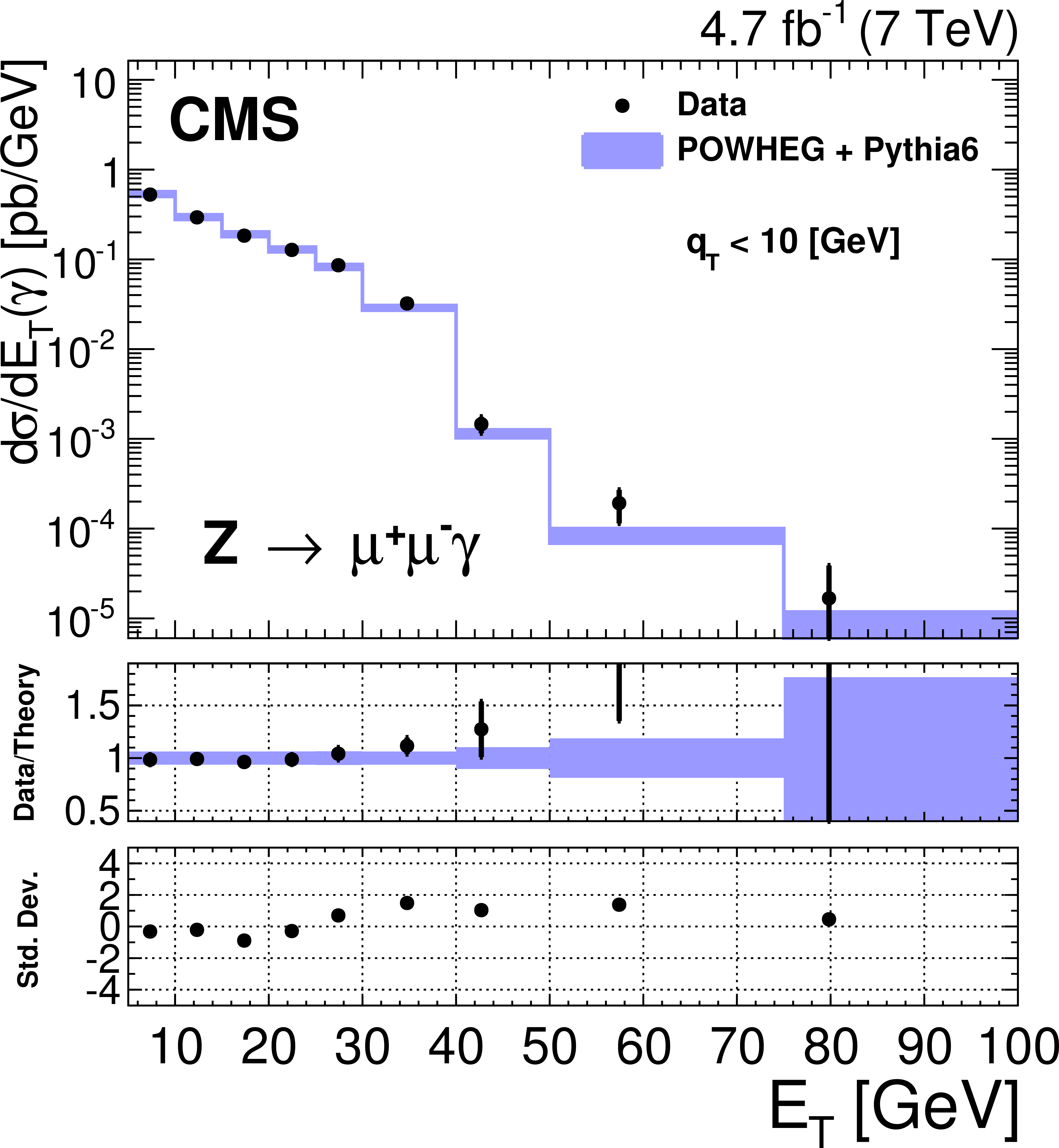
Measured differential cross sections $\mathrm{d}\sigma / \mathrm{d} E_{\mathrm{T}}$ and $\mathrm{d}\sigma / \mathrm{d} \Delta R_{\mu\gamma}$ for $q_{\mathrm{T}} <$ 10 GeV (a, b) and $q_{\mathrm{T}} >$ 50 GeV (c, d). The dots with error bars represent the data, and the shaded bands represent the POWHEG+PYTHIA calculation including theoretical uncertainties. The bottom panels display the ratio of data to the MC expectation. A bin-centering procedure has been applied. |

png pdf |
Figure 5-b:
Measured differential cross sections $\mathrm{d}\sigma / \mathrm{d} E_{\mathrm{T}}$ and $\mathrm{d}\sigma / \mathrm{d} \Delta R_{\mu\gamma}$ for $q_{\mathrm{T}} <$ 10 GeV (a, b) and $q_{\mathrm{T}} >$ 50 GeV (c, d). The dots with error bars represent the data, and the shaded bands represent the POWHEG+PYTHIA calculation including theoretical uncertainties. The bottom panels display the ratio of data to the MC expectation. A bin-centering procedure has been applied. |
png pdf |
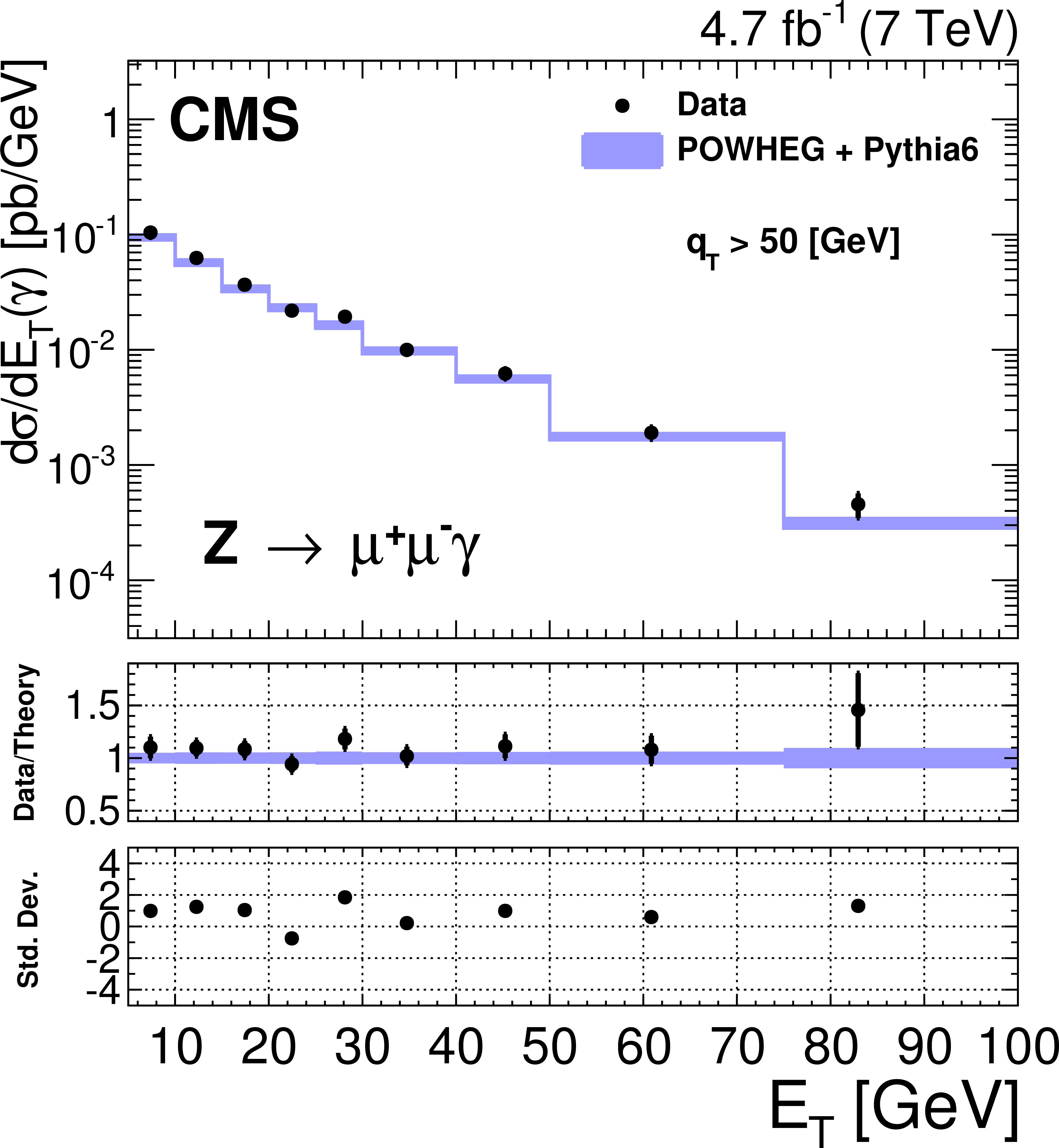
Figure 5-c:
Measured differential cross sections $\mathrm{d}\sigma / \mathrm{d} E_{\mathrm{T}}$ and $\mathrm{d}\sigma / \mathrm{d} \Delta R_{\mu\gamma}$ for $q_{\mathrm{T}} <$ 10 GeV (a, b) and $q_{\mathrm{T}} >$ 50 GeV (c, d). The dots with error bars represent the data, and the shaded bands represent the POWHEG+PYTHIA calculation including theoretical uncertainties. The bottom panels display the ratio of data to the MC expectation. A bin-centering procedure has been applied. |
png pdf |
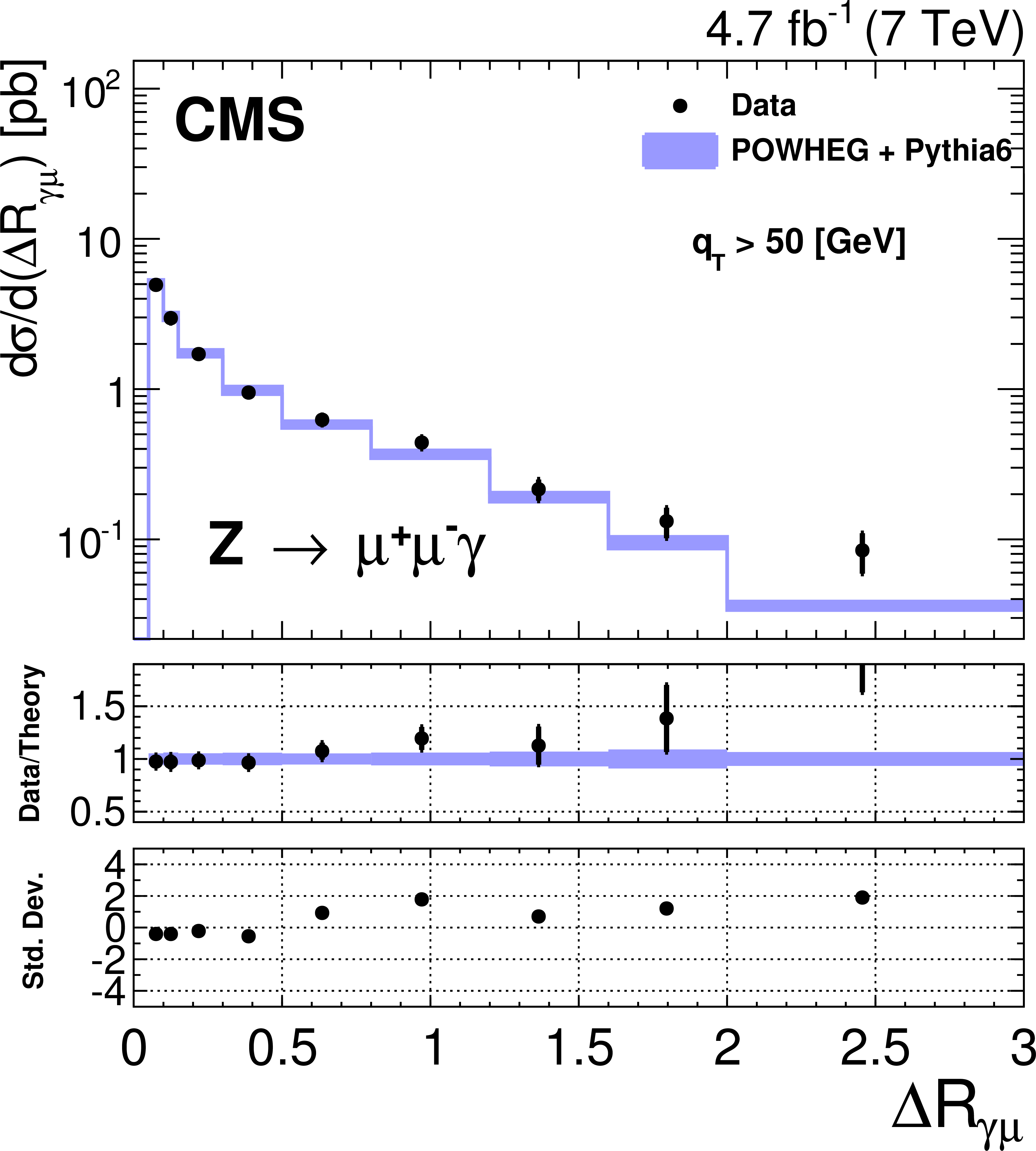
Figure 5-d:
Measured differential cross sections $\mathrm{d}\sigma / \mathrm{d} E_{\mathrm{T}}$ and $\mathrm{d}\sigma / \mathrm{d} \Delta R_{\mu\gamma}$ for $q_{\mathrm{T}} <$ 10 GeV (a, b) and $q_{\mathrm{T}} >$ 50 GeV (c, d). The dots with error bars represent the data, and the shaded bands represent the POWHEG+PYTHIA calculation including theoretical uncertainties. The bottom panels display the ratio of data to the MC expectation. A bin-centering procedure has been applied. |
png pdf |
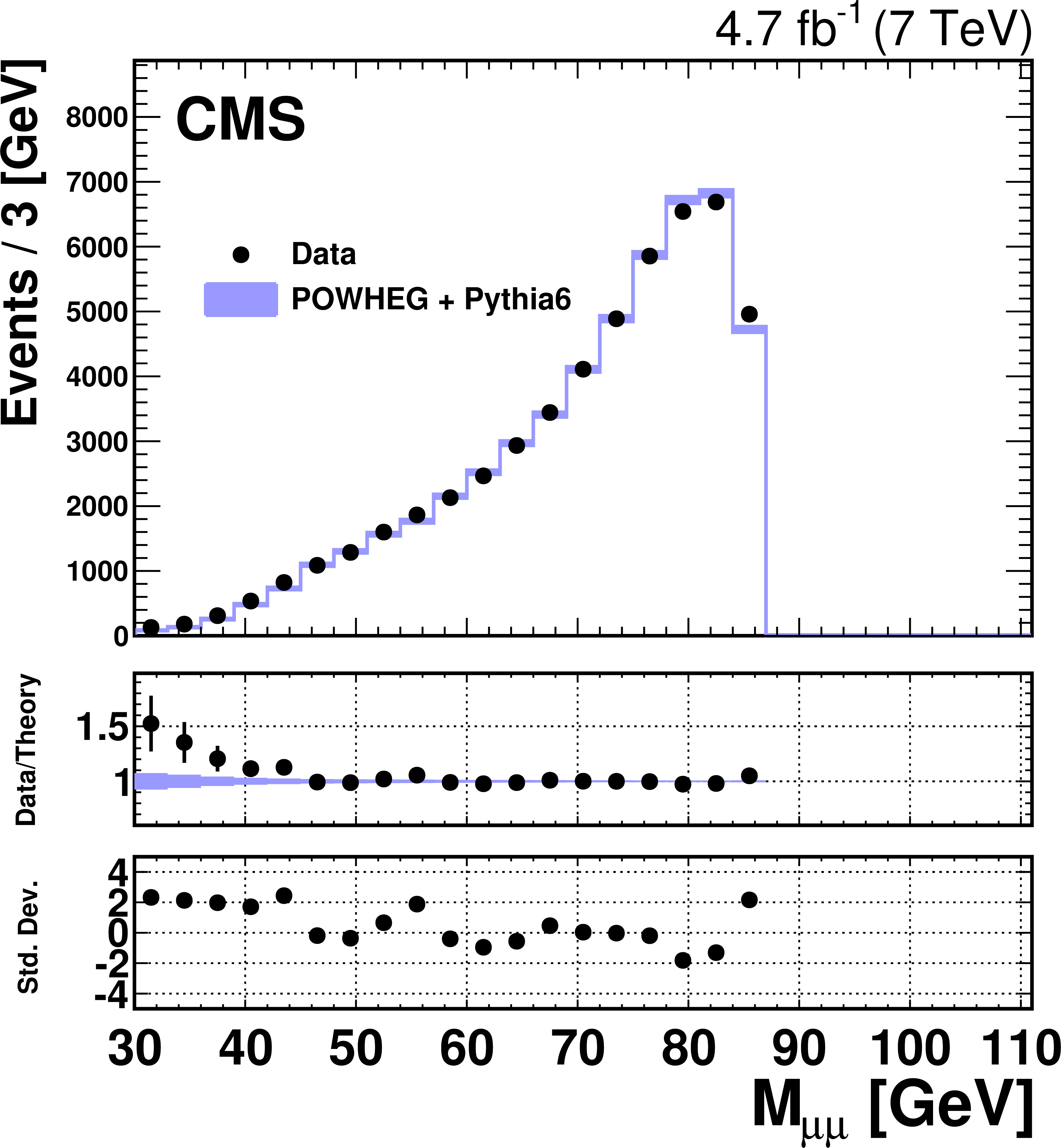
Figure 6-a:
Distributions of the dimuon mass $M_{\mu \mu}$ (a) and the three-body mass $M_{\mu \mu \gamma}$ (b). The dots with error bars represent the data, and the shaded bands represent the POWHEG+PYTHIA prediction. The bottom panels display the ratio of data to the MC expectation. |
png pdf |
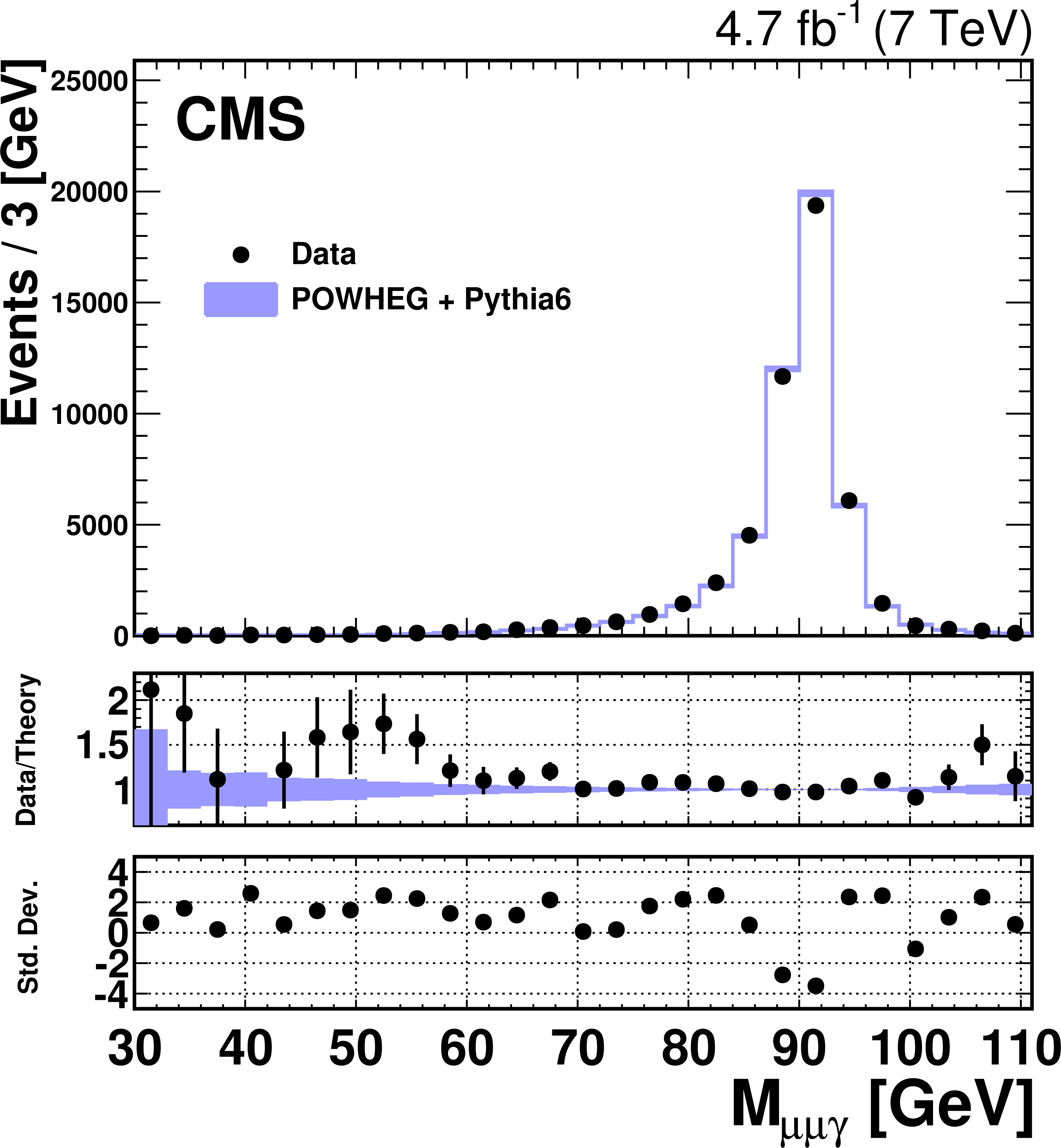
Figure 6-b:
Distributions of the dimuon mass $M_{\mu \mu}$ (a) and the three-body mass $M_{\mu \mu \gamma}$ (b). The dots with error bars represent the data, and the shaded bands represent the POWHEG+PYTHIA prediction. The bottom panels display the ratio of data to the MC expectation. |
| Tables | |
png pdf |
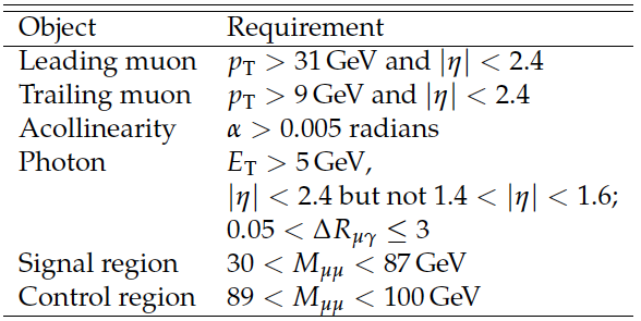
Table 1:
Summary of kinematic and fiducial event requirements |
png pdf |
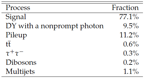
Table 2:
Composition of the signal sample. The simulation has been tuned to reproduce the data in the control region. |

png pdf |
Table 3:
Relative systematic uncertainties for $\mathrm{d} \sigma / \mathrm{d} E_{\mathrm{T}}$ (in percent). |
png pdf |
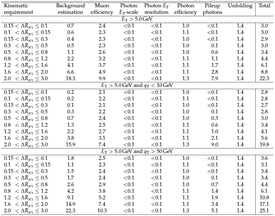
Table 4:
Relative systematic uncertainties for $\mathrm{d} \sigma / \mathrm{d} \Delta R_{\mu\gamma}$ (in percent). |

png pdf |
Table 5:
Measured differential cross section $\mathrm{d} \sigma / \mathrm{d} E_{\mathrm{T}}$ in pb/GeV. For the data values, the first uncertainty is statistical and the second is systematic. For the theory values, the uncertainty combines statistical, PDF, and renormalization/factorization scale components. |
png pdf |
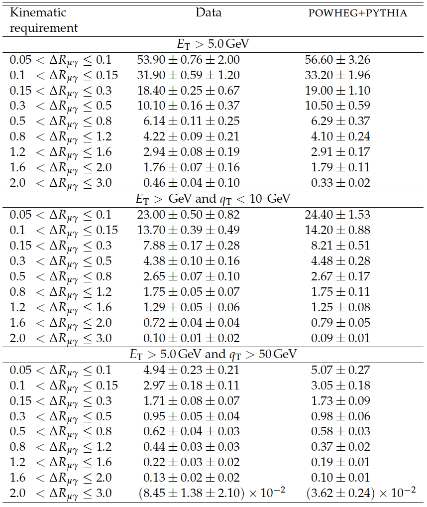
Table 6:
Measured differential cross section $\mathrm{d} \sigma / \mathrm{d} \Delta R_{\mu\gamma}$ in pb. For the data values, the first uncertainty is statistical and the second is systematic. For the theory values, the uncertainty combines statistical, PDF, and renormalization/factorization scale components. |
|
|
Compact Muon Solenoid LHC, CERN |
|

|

|

|

|

|