

Compact Muon Solenoid
LHC, CERN
| CMS-EXO-13-009 ; CERN-PH-EP-2014-076 | ||
| Search for massive resonances decaying into pairs of boosted bosons in semi-leptonic final states at $\sqrt{s}$ = 8 TeV | ||
| CMS Collaboration | ||
| 14 May 2014 | ||
| J. High Energy Phys. 08 (2014) 174 | ||
| Abstract: A search for new resonances decaying to WW, ZZ, or WZ is presented. Final states are considered in which one of the vector bosons decays leptonically and the other hadronically. Results are based on data corresponding to an integrated luminosity of 19.7 inverse-femtobarn recorded in proton-proton collisions at $\sqrt{s}$ = 8 TeV with the CMS detector at the CERN LHC. Techniques aiming at identifying jet substructures are used to analyze signal events in which the hadronization products from the decay of highly boosted W or Z bosons are contained within a single reconstructed jet. Upper limits on the production of generic WW, ZZ, or WZ resonances are set as a function of the resonance mass and width. We increase the sensitivity of the analysis by statistically combining the results of this search with a complementary study of the all-hadronic final state. Upper limits at 95% confidence level are set on the bulk graviton production cross section in the range from 700 to 10 inverse-femtobarns for resonance masses between 600 and 2500 GeV, respectively. These limits on the bulk graviton model are the most stringent to date in the diboson final state. | ||
| Links: e-print arXiv:1405.3447 [hep-ex] (PDF) ; CDS record ; inSPIRE record ; Public twiki page ; HepData record ; CADI line (restricted) ; | ||
| Figures | |
png pdf |
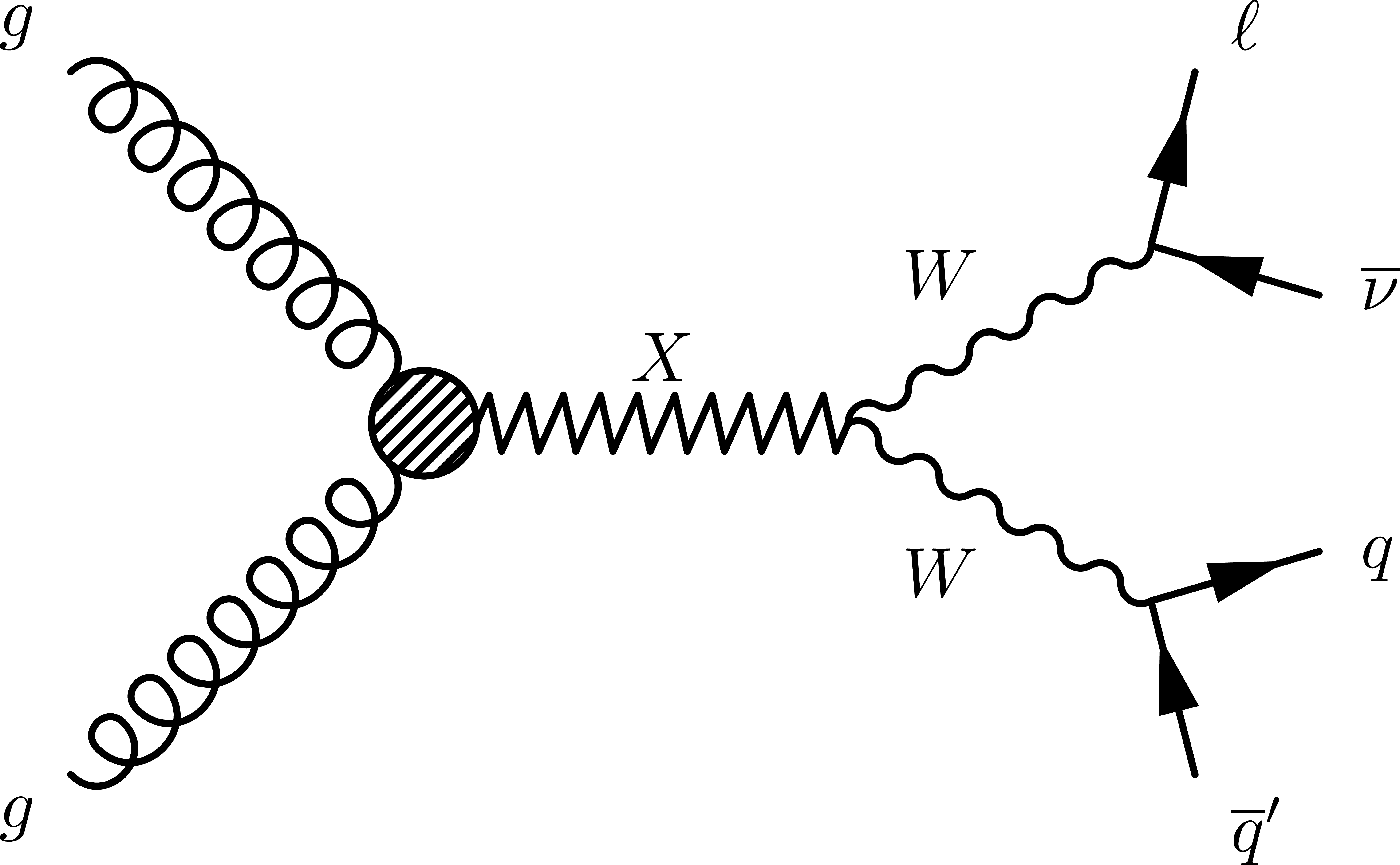
Figure 1-a:
Two Feynman diagrams for the production of a generic resonance X decaying to some of the final states considered in this study. |
png pdf |
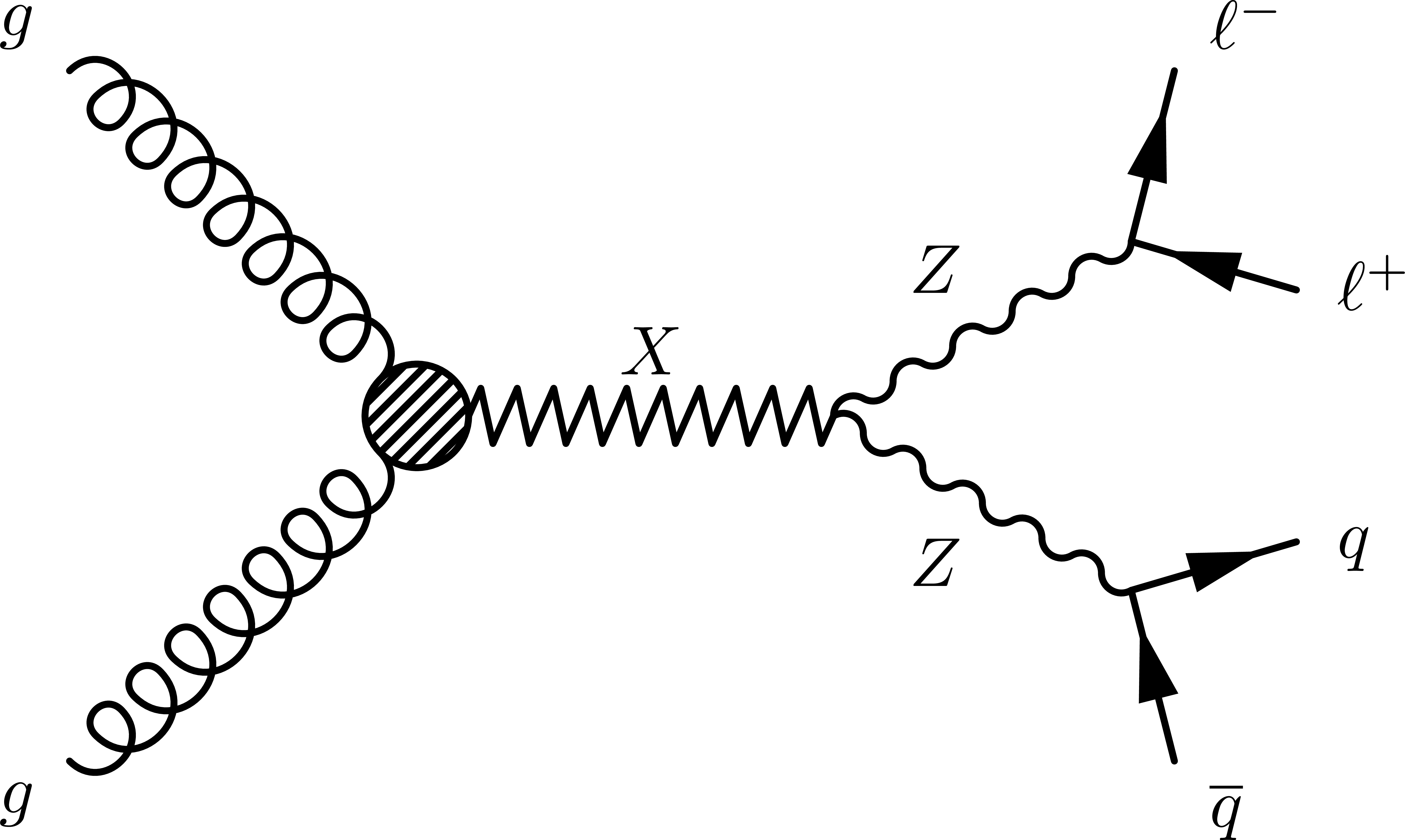
Figure 1-b:
Two Feynman diagrams for the production of a generic resonance X decaying to some of the final states considered in this study. |
png pdf |
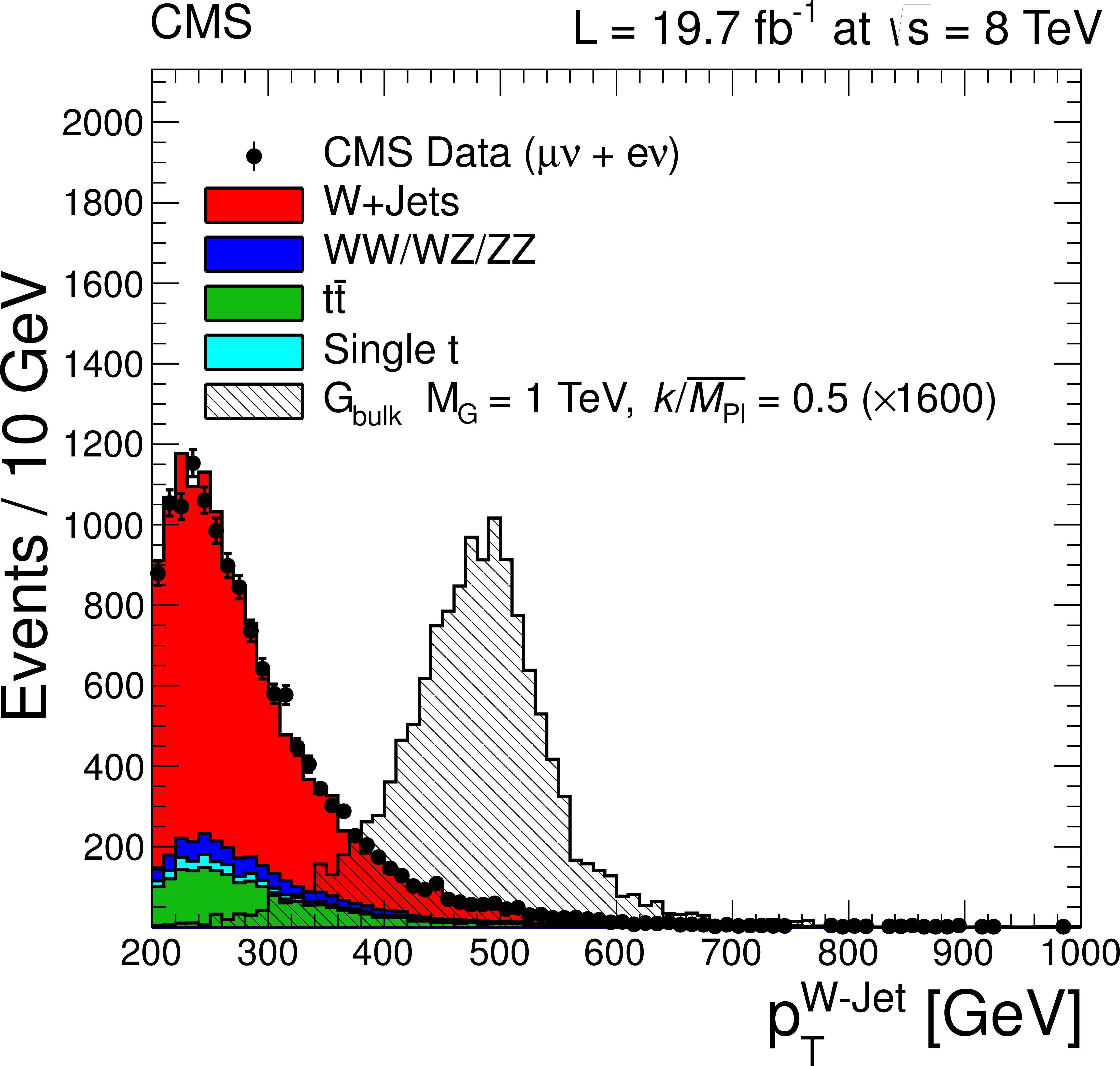
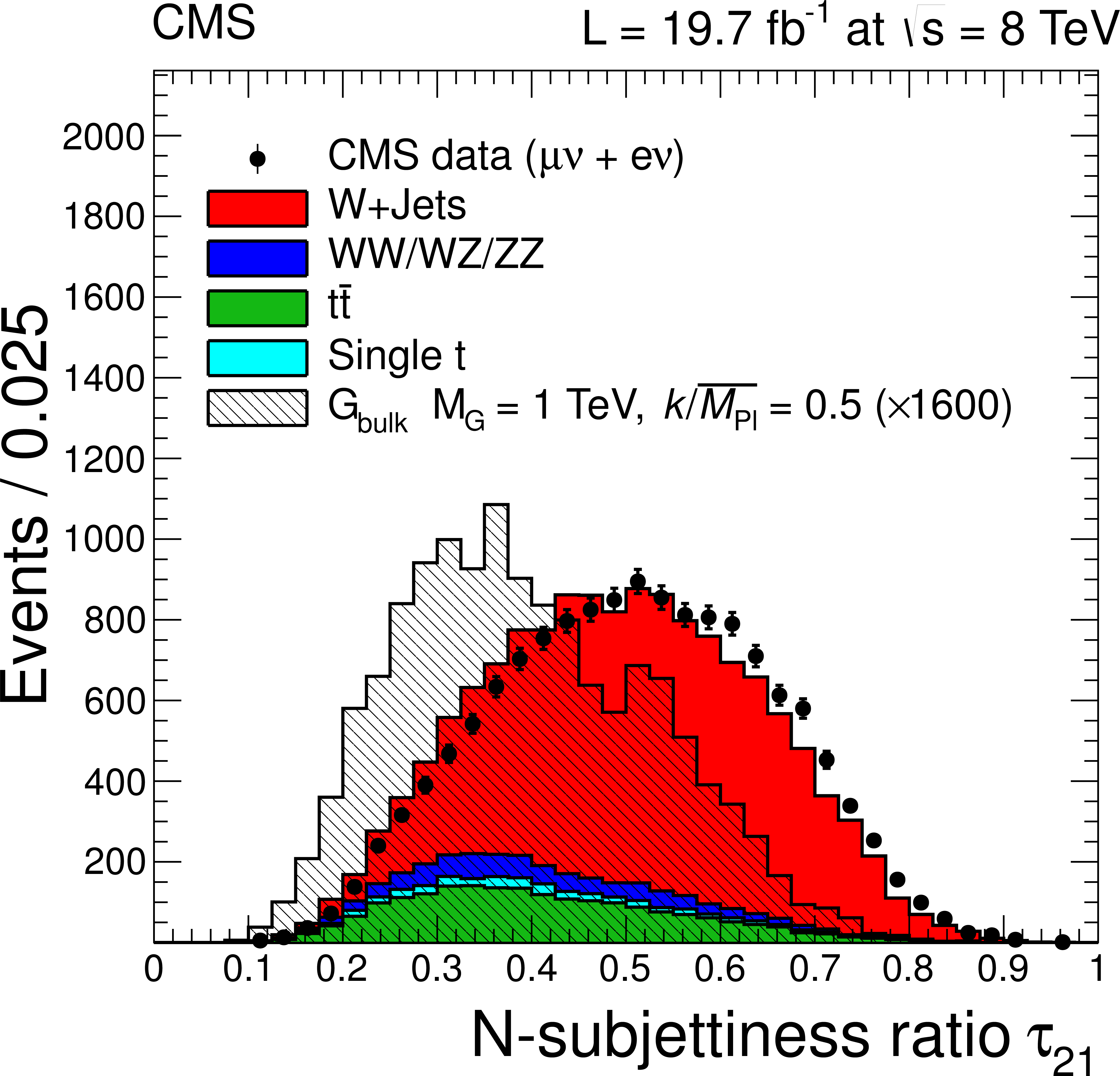
Figure 2-a:
Hadronic W $ {p_{\mathrm {T}}} $ and N-subjettiness ratio $\tau _{21}$ distributions for the combined muon and electron channels and with 65 $< {m_{\text {jet}}}< $ 105 GeV. The VV, $ {\mathrm {t}\overline {\mathrm {t}}} $, and single-t backgrounds are taken from simulation and are normalized to the integrated luminosity of the data sample. The W+jets background is rescaled such that the total number of background events matches the number of events in data. The signal is scaled by a factor of 1600 for better visualization. |
png pdf |
Figure 2-b:
Hadronic W $ {p_{\mathrm {T}}} $ and N-subjettiness ratio $\tau _{21}$ distributions for the combined muon and electron channels and with 65 $< {m_{\text {jet}}}< $ 105 GeV. The VV, $ {\mathrm {t}\overline {\mathrm {t}}} $, and single-t backgrounds are taken from simulation and are normalized to the integrated luminosity of the data sample. The W+jets background is rescaled such that the total number of background events matches the number of events in data. The signal is scaled by a factor of 1600 for better visualization. |
png pdf |
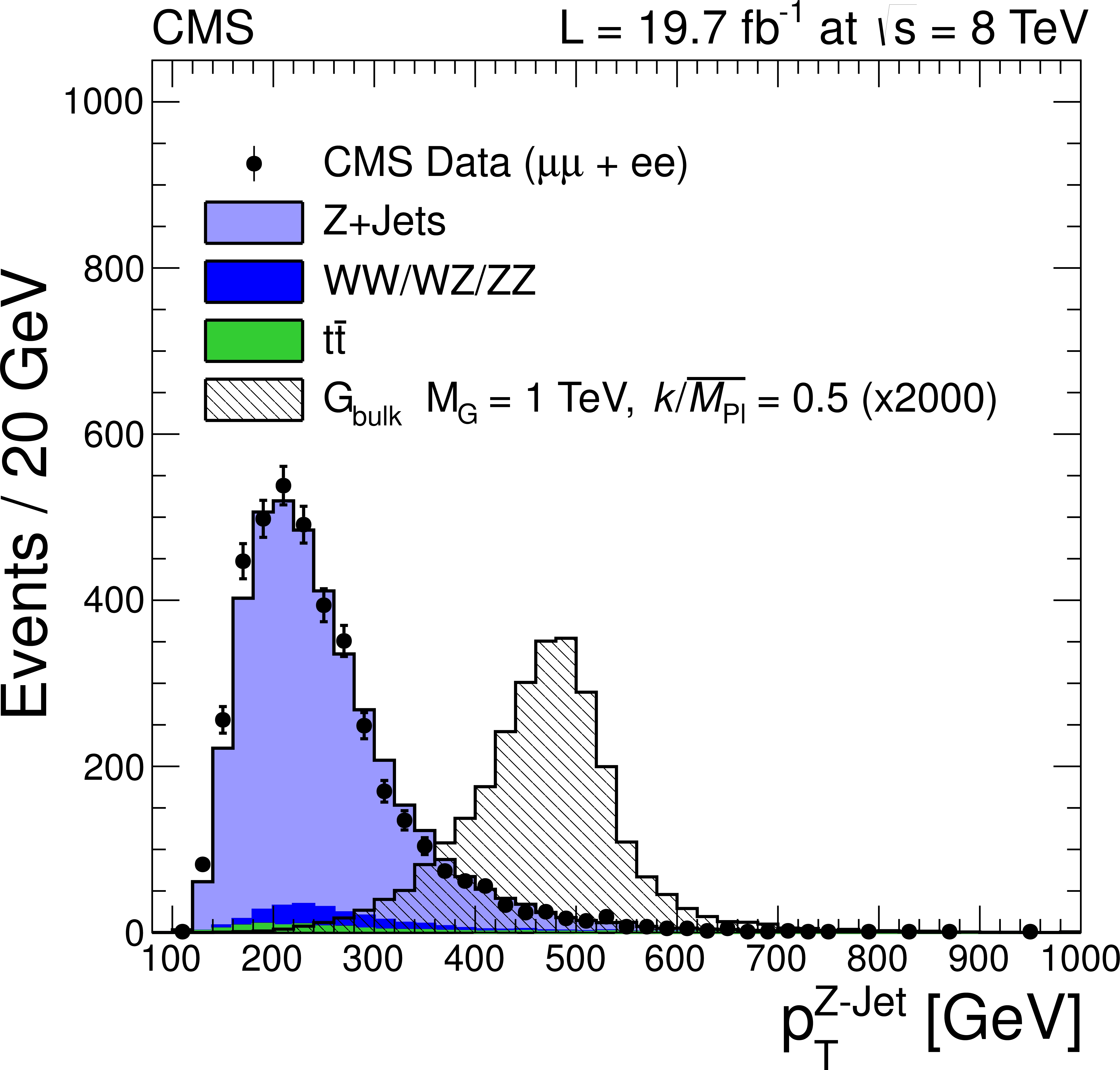
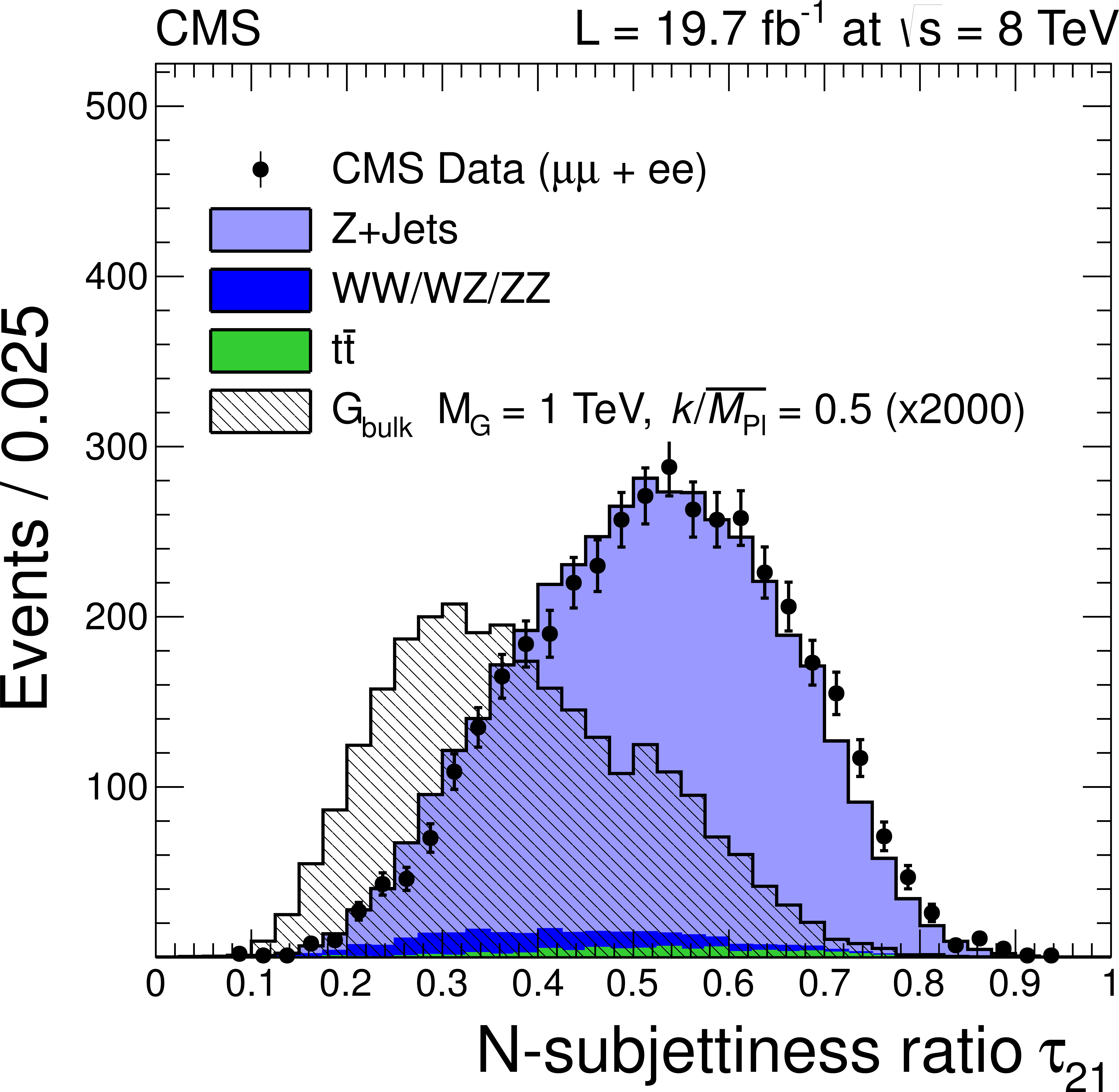
Figure 3-a:
Hadronic Z $ {p_{\mathrm {T}}} $ and N-subjettiness ratio $\tau _{21}$ distributions for the combined muon and electron channels and with 70 $< {m_{\text {jet}}}<$ 110 GeV. The VV and $ {\mathrm {t}\overline {\mathrm {t}}} $ backgrounds are taken from simulation and are normalized to the integrated luminosity of the data sample. The Z+jets background is rescaled such that the total number of background events matches the number of events in data. The signal is scaled by a factor of 2000 for better visualization. |
png pdf |
Figure 3-b:
Hadronic Z $ {p_{\mathrm {T}}} $ and N-subjettiness ratio $\tau _{21}$ distributions for the combined muon and electron channels and with 70 $< {m_{\text {jet}}}<$ 110 GeV. The VV and $ {\mathrm {t}\overline {\mathrm {t}}} $ backgrounds are taken from simulation and are normalized to the integrated luminosity of the data sample. The Z+jets background is rescaled such that the total number of background events matches the number of events in data. The signal is scaled by a factor of 2000 for better visualization. |

png pdf |
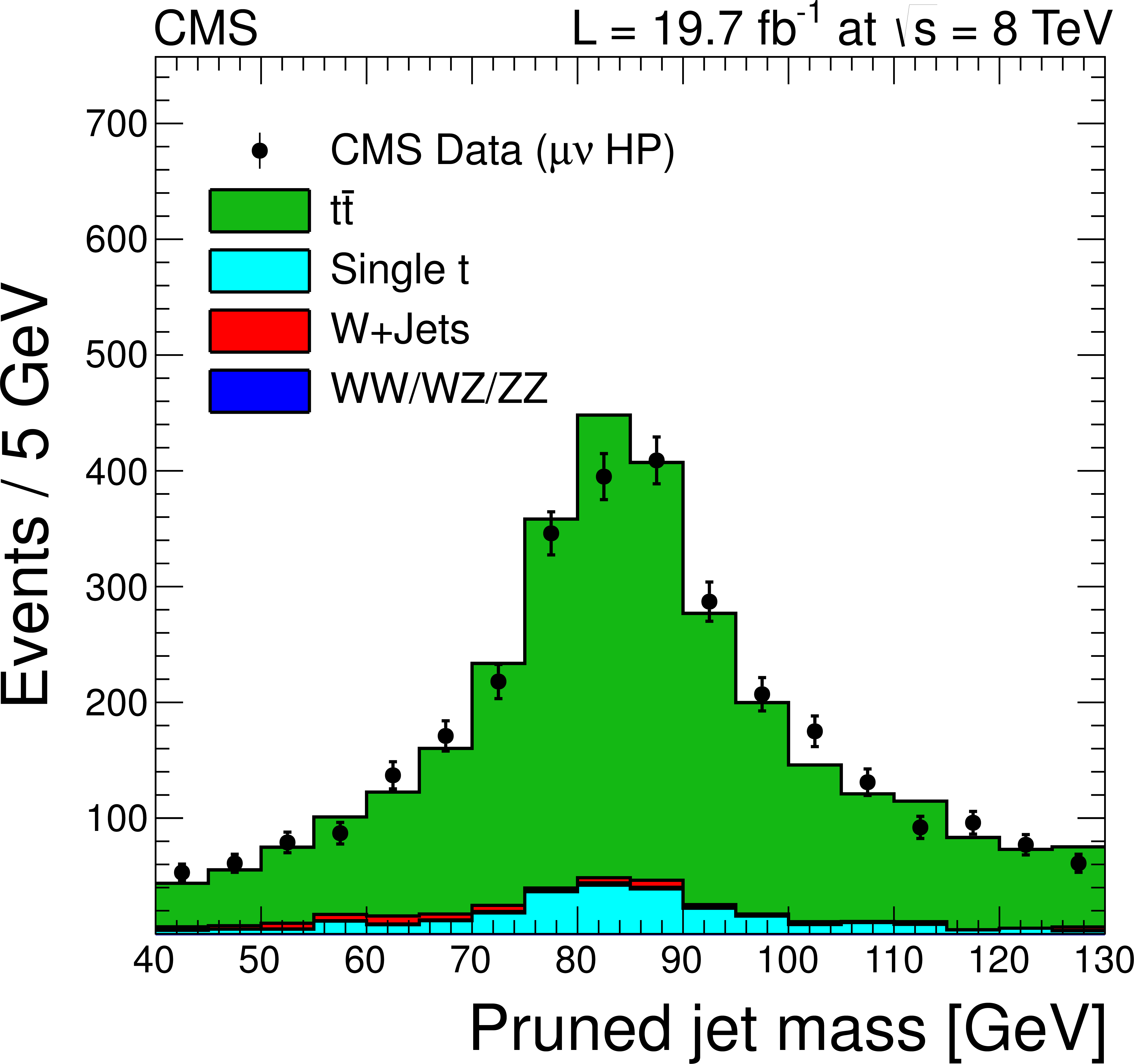
Figure 4-a:
Distributions from the top-quark enriched control sample in the muon channel. a: N-subjettiness ratio $\tau _{21}$, b: ${m_{\text {jet}}}$ after requiring $\tau _{21}<$ 0.5. The distributions show some disagreement between data and simulation. The simulation is corrected for these discrepancies using the method based on data. This approach ensures that the analysis is robust against differences between data and simulation, independent of their sources. |
png pdf |
Figure 4-b:
Distributions from the top-quark enriched control sample in the muon channel. a: N-subjettiness ratio $\tau _{21}$, b: ${m_{\text {jet}}}$ after requiring $\tau _{21}<$ 0.5. The distributions show some disagreement between data and simulation. The simulation is corrected for these discrepancies using the method based on data. This approach ensures that the analysis is robust against differences between data and simulation, independent of their sources. |
png pdf |
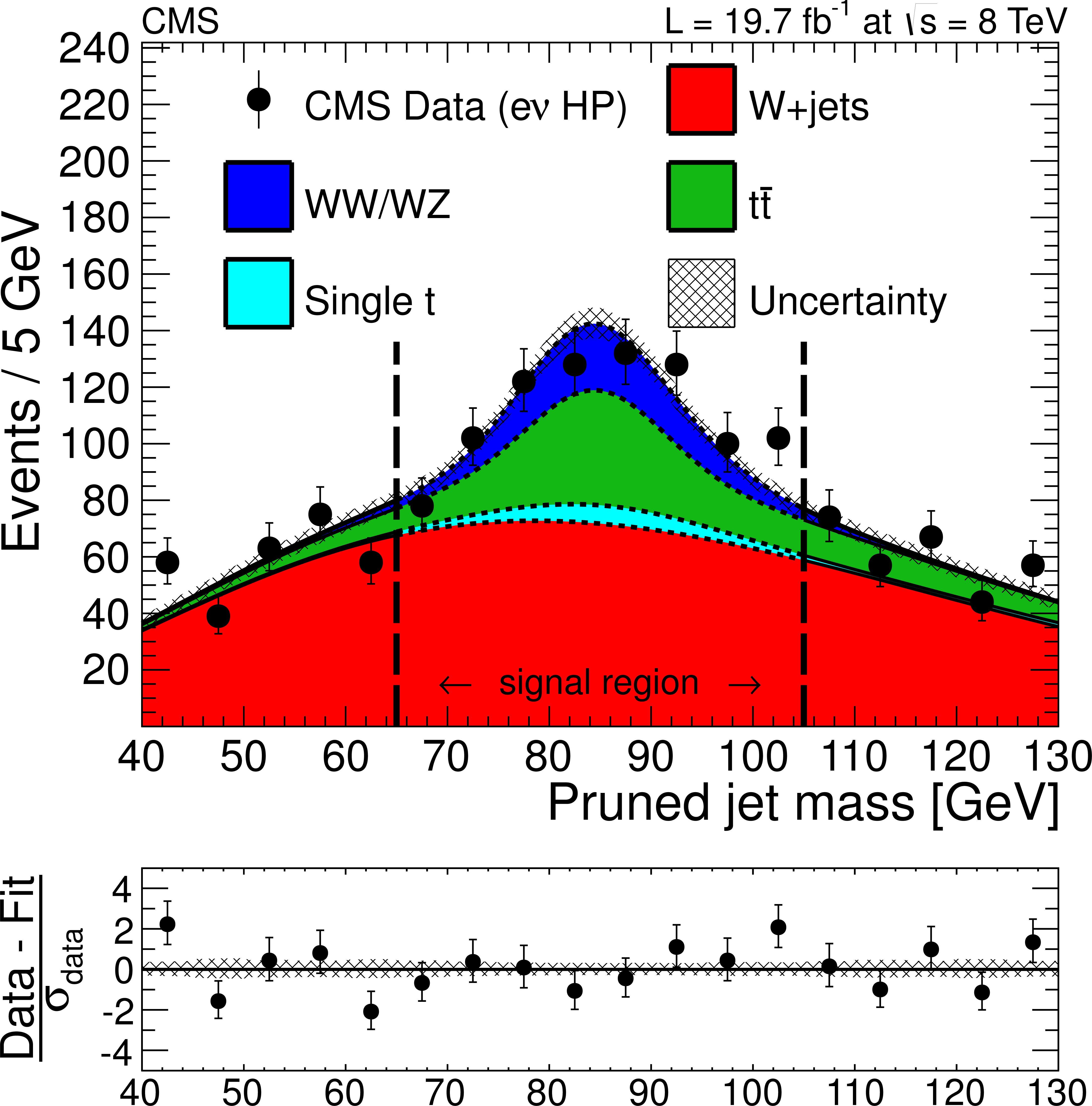
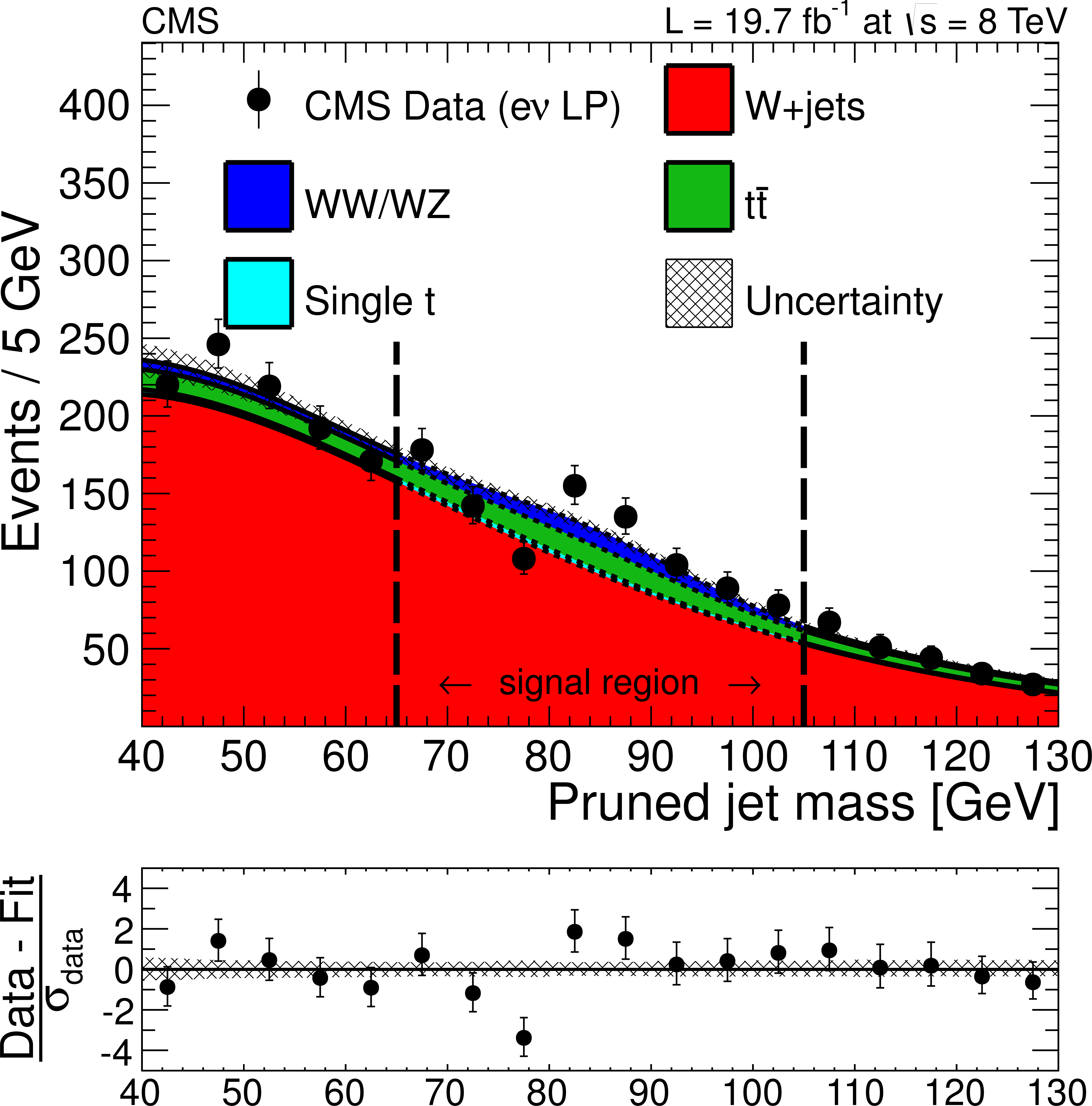
Figure 5-a:
Distributions of the pruned jet mass, $ {m_{\text {jet}}}$, in the $ {\ell \nu }$+V-jet analysis in the electron channel. The a (b) panel shows the distribution for the HP (LP) category. All selections are applied except the final $ {m_{\text {jet}}}$ signal window requirement. Data are shown as black markers. The prediction of the non-resonant W+jets background comes from a fit excluding the signal region (between the vertical dashed lines), while the predictions for the minor backgrounds come from the simulation. The MC resonant shapes are corrected using the differences between data and simulation in the W peak position and width measured in the $ {\mathrm {t}\overline {\mathrm {t}}} $ control region. At the bottom of each plot, the bin-by-bin fit residuals, (data-fit)/$\sigma _\text {data}$, are shown together with the uncertainty band of the fit normalized by $\sigma _\text {data}$. |
png pdf |
Figure 5-b:
Distributions of the pruned jet mass, $ {m_{\text {jet}}}$, in the $ {\ell \nu }$+V-jet analysis in the electron channel. The a (b) panel shows the distribution for the HP (LP) category. All selections are applied except the final $ {m_{\text {jet}}}$ signal window requirement. Data are shown as black markers. The prediction of the non-resonant W+jets background comes from a fit excluding the signal region (between the vertical dashed lines), while the predictions for the minor backgrounds come from the simulation. The MC resonant shapes are corrected using the differences between data and simulation in the W peak position and width measured in the $ {\mathrm {t}\overline {\mathrm {t}}} $ control region. At the bottom of each plot, the bin-by-bin fit residuals, (data-fit)/$\sigma _\text {data}$, are shown together with the uncertainty band of the fit normalized by $\sigma _\text {data}$. |

png pdf |
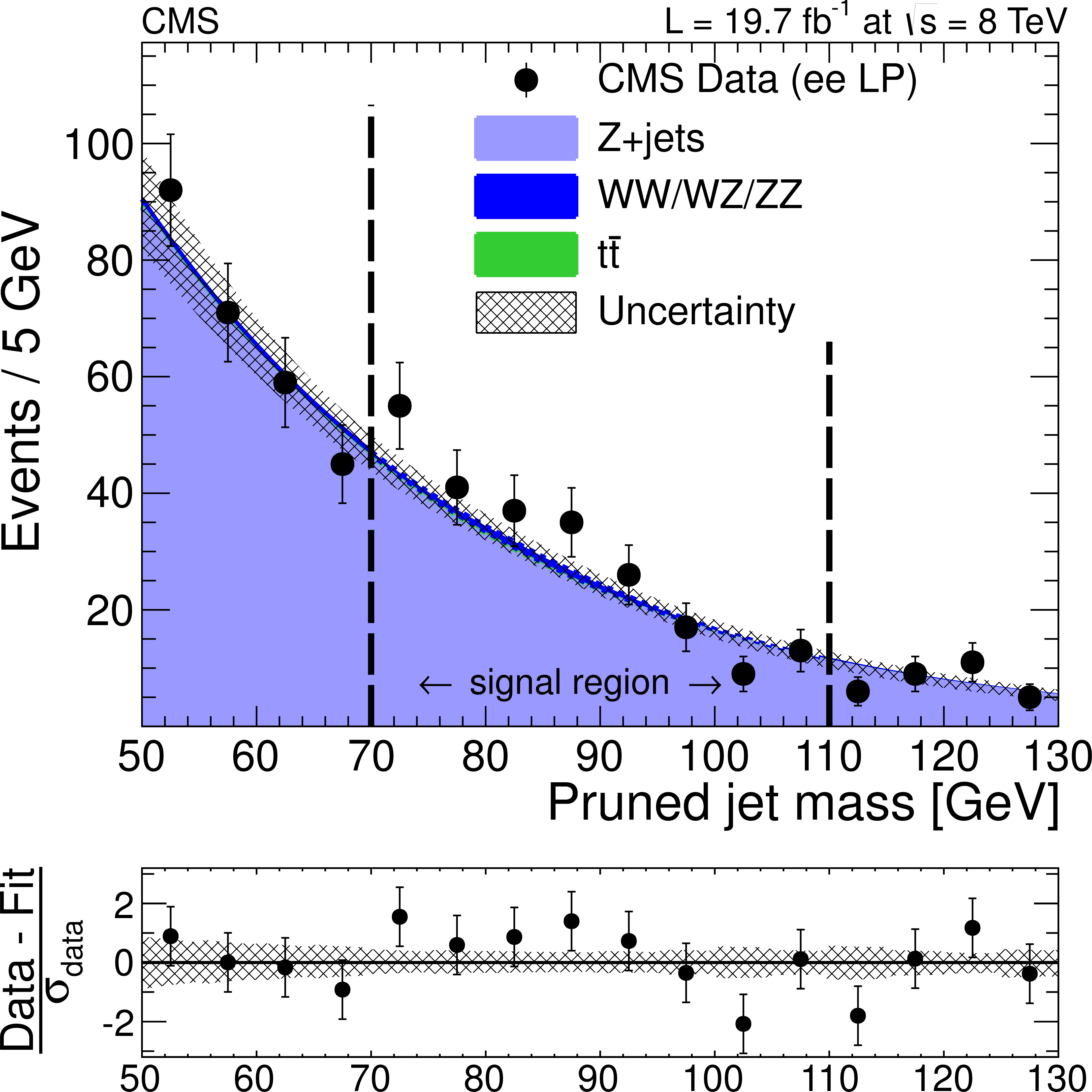
Figure 6-a:
Distributions of the pruned jet mass, $ {m_{\text {jet}}}$, in the $ {\ell \ell }$+V-jet analysis in the electron channel. The a (b) panel shows the distribution for the HP (LP) category. All selections are applied except the final $ {m_{\text {jet}}}$ signal window requirement. Data are shown as black markers. The prediction of the non-resonant Z+jets background comes from a fit excluding the signal region (between the vertical dashed lines), while the predictions for the minor backgrounds come from the simulation. The MC resonant shapes are corrected using the differences between data and simulation in the W peak position and width measured in the $ {\mathrm {t}\overline {\mathrm {t}}} $ control region. At the bottom of each plot, the bin-by-bin fit residuals, (data-fit)/$\sigma _\text {data}$, are shown together with the uncertainty band of the fit normalized by $\sigma _\text {data}$. |
png pdf |
Figure 6-b:
Distributions of the pruned jet mass, $ {m_{\text {jet}}}$, in the $ {\ell \ell }$+V-jet analysis in the electron channel. The a (b) panel shows the distribution for the HP (LP) category. All selections are applied except the final $ {m_{\text {jet}}}$ signal window requirement. Data are shown as black markers. The prediction of the non-resonant Z+jets background comes from a fit excluding the signal region (between the vertical dashed lines), while the predictions for the minor backgrounds come from the simulation. The MC resonant shapes are corrected using the differences between data and simulation in the W peak position and width measured in the $ {\mathrm {t}\overline {\mathrm {t}}} $ control region. At the bottom of each plot, the bin-by-bin fit residuals, (data-fit)/$\sigma _\text {data}$, are shown together with the uncertainty band of the fit normalized by $\sigma _\text {data}$. |
png pdf |
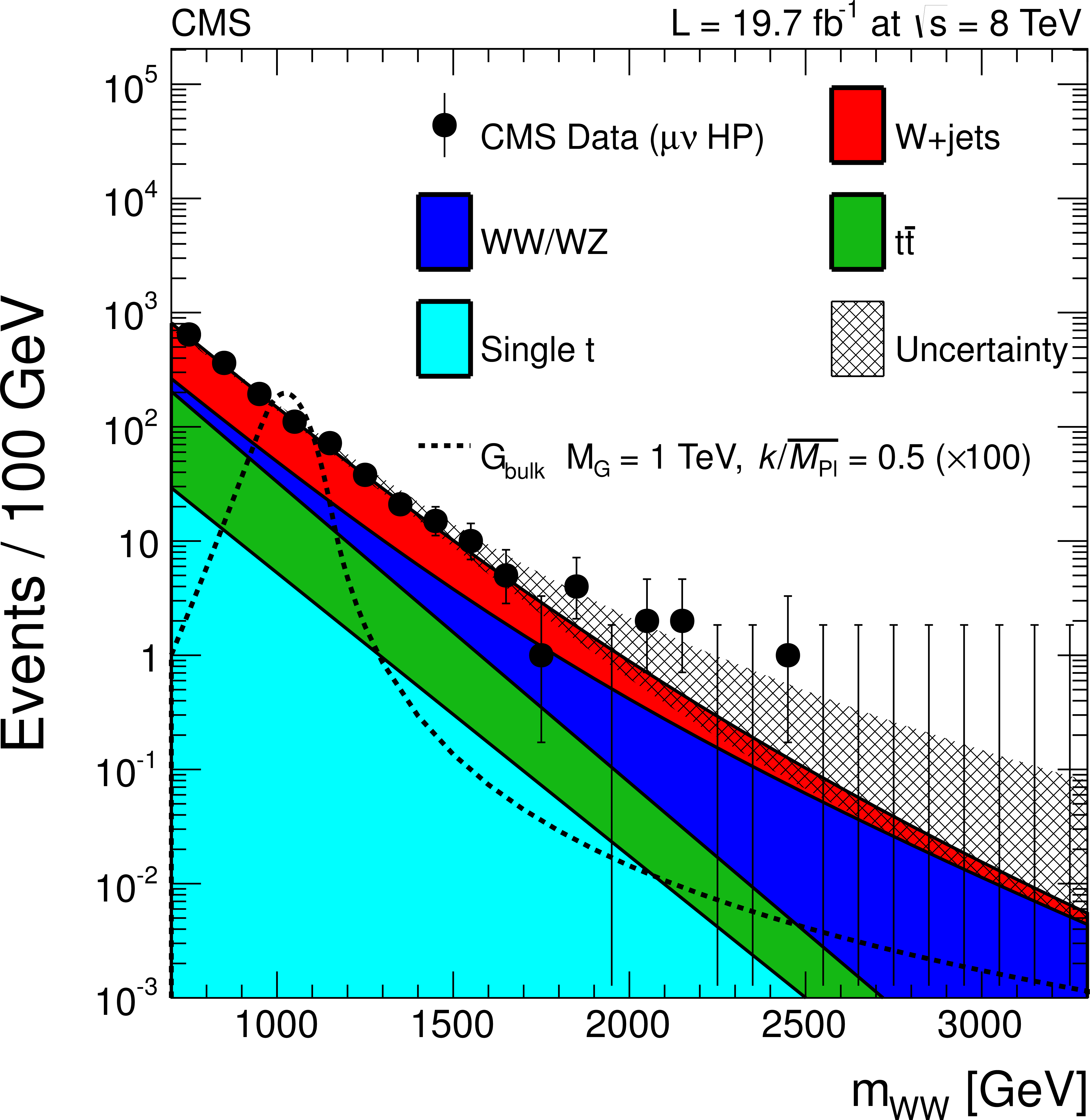
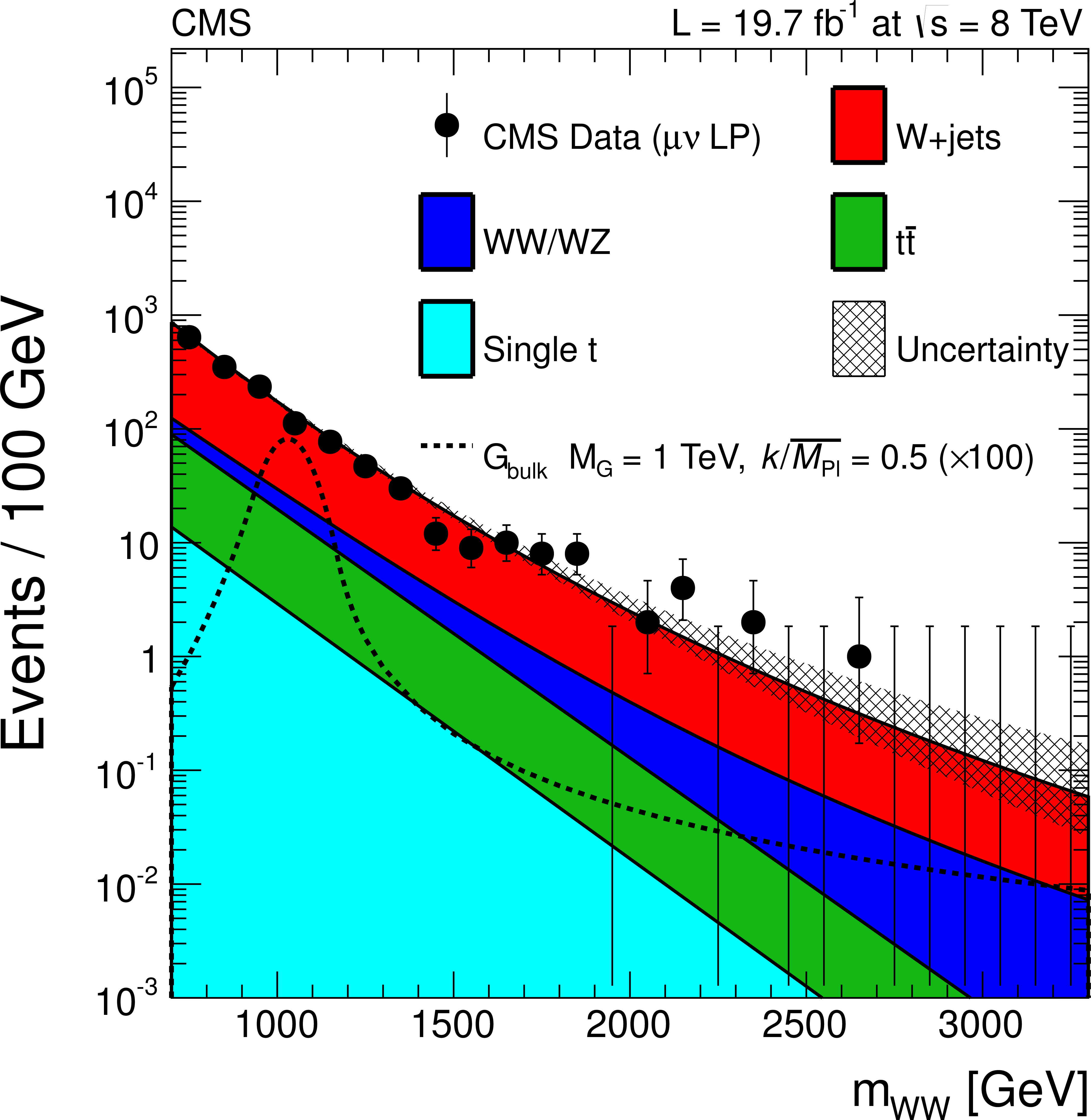
Figure 7-a:
Final distributions in $ {m_{ {\mathrm {W}} {\mathrm {W}} }} $ for data and expected backgrounds for both the muon (top) and the electron (bottom) channels, high-purity (a) and low-purity (b) categories. The 68% error bars for Poisson event counts are obtained from the Neyman construction. Also shown is a hypothetical bulk graviton signal with mass of 1000 GeV and $ {k/\overline {M}_\mathrm {Pl}} =$ 0.5. The normalization of the signal distribution is scaled up by a factor of 100 for a better visualization. |
png pdf |
Figure 7-b:
Final distributions in $ {m_{ {\mathrm {W}} {\mathrm {W}} }} $ for data and expected backgrounds for both the muon (top) and the electron (bottom) channels, high-purity (a) and low-purity (b) categories. The 68% error bars for Poisson event counts are obtained from the Neyman construction. Also shown is a hypothetical bulk graviton signal with mass of 1000 GeV and $ {k/\overline {M}_\mathrm {Pl}} =$ 0.5. The normalization of the signal distribution is scaled up by a factor of 100 for a better visualization. |
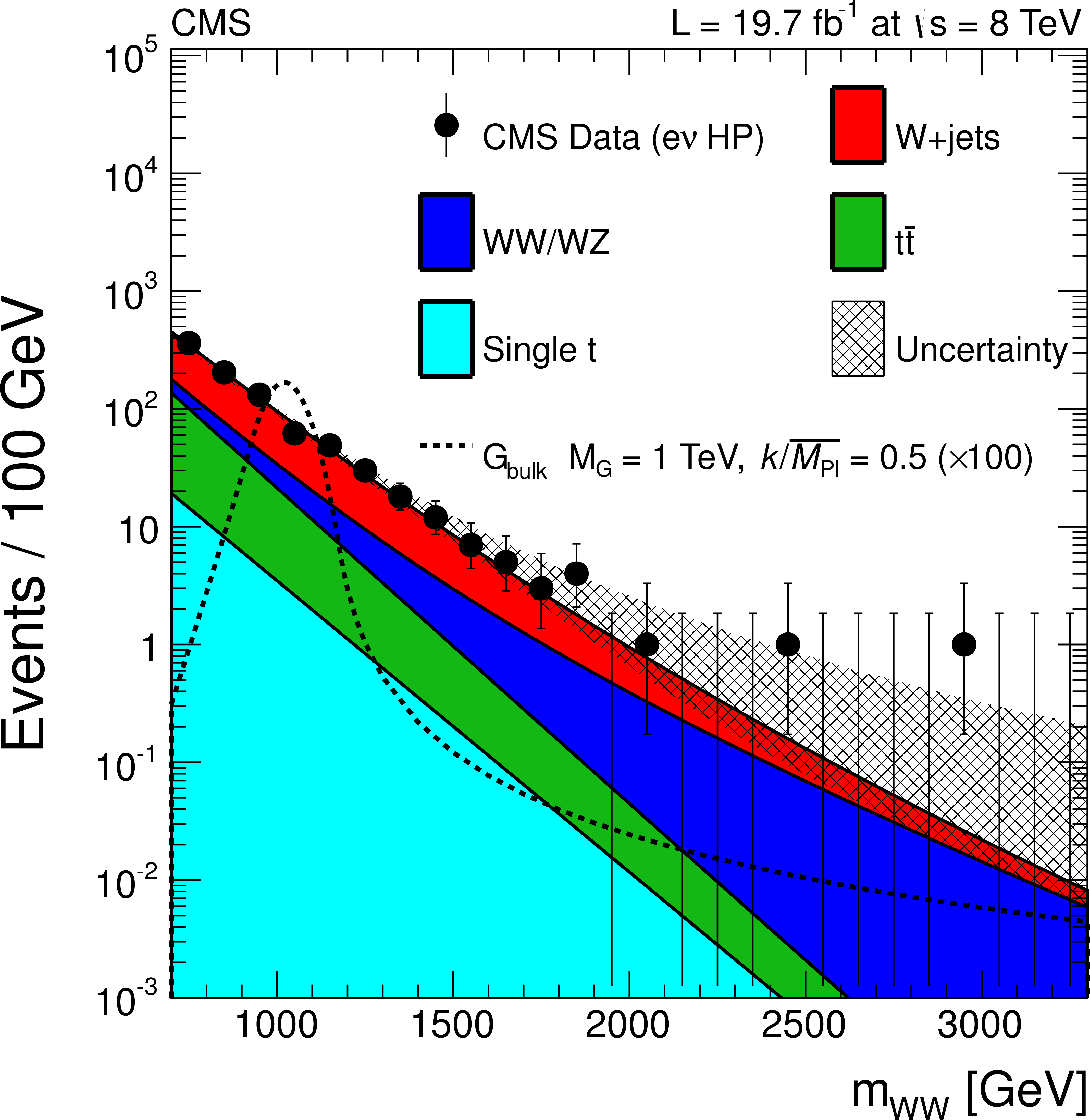
png pdf |
Figure 7-c:
Final distributions in $ {m_{ {\mathrm {W}} {\mathrm {W}} }} $ for data and expected backgrounds for both the muon (top) and the electron (bottom) channels, high-purity (a) and low-purity (b) categories. The 68% error bars for Poisson event counts are obtained from the Neyman construction. Also shown is a hypothetical bulk graviton signal with mass of 1000 GeV and $ {k/\overline {M}_\mathrm {Pl}} =$ 0.5. The normalization of the signal distribution is scaled up by a factor of 100 for a better visualization. |

png pdf |
Figure 7-d:
Final distributions in $ {m_{ {\mathrm {W}} {\mathrm {W}} }} $ for data and expected backgrounds for both the muon (top) and the electron (bottom) channels, high-purity (a) and low-purity (b) categories. The 68% error bars for Poisson event counts are obtained from the Neyman construction. Also shown is a hypothetical bulk graviton signal with mass of 1000 GeV and $ {k/\overline {M}_\mathrm {Pl}} =$ 0.5. The normalization of the signal distribution is scaled up by a factor of 100 for a better visualization. |

png pdf |
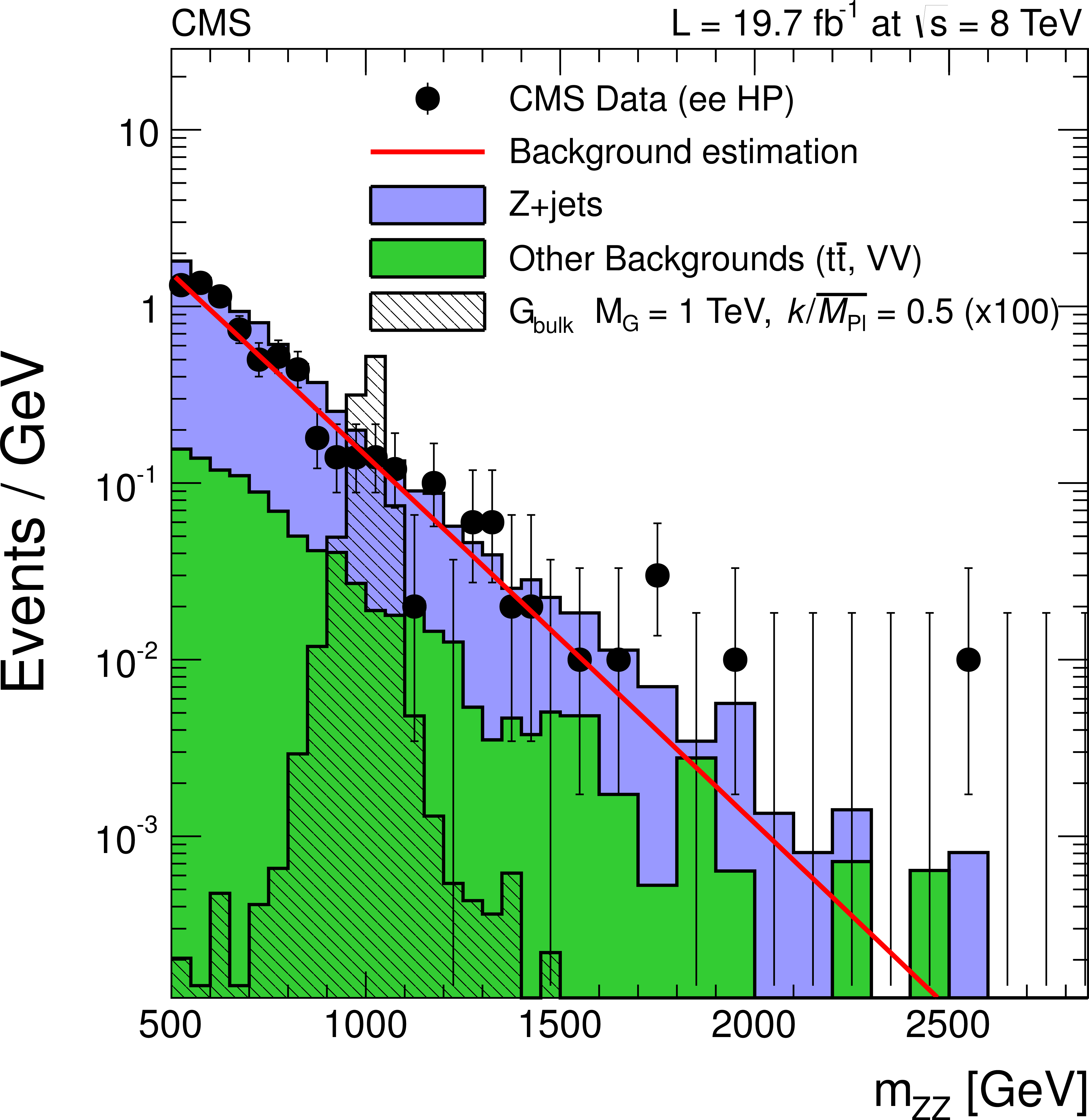
Figure 8-a:
Final distributions in $ {m_{ {\mathrm {Z}} {\mathrm {Z}} }} $ for data and expected backgrounds for both the muon (a,b) and the electron (c,d) channels, high-purity (a,c) and low-purity (b,d) categories. Points with error bars show distributions of data; solid histograms depict the different components of the background expectation from simulated events. The 68% error bars for Poisson event counts are obtained from the Neyman construction. Also shown is a hypothetical bulk graviton signal with mass of 1000 GeV and $ {k/\overline {M}_\mathrm {Pl}} =$ 0.5. The normalization of the signal distribution is scaled up by a factor of 100 for a better visualization. The solid line shows the central value of the background predicted from the sideband extrapolation procedure. |

png pdf |
Figure 8-b:
Final distributions in $ {m_{ {\mathrm {Z}} {\mathrm {Z}} }} $ for data and expected backgrounds for both the muon (a,b) and the electron (c,d) channels, high-purity (a,c) and low-purity (b,d) categories. Points with error bars show distributions of data; solid histograms depict the different components of the background expectation from simulated events. The 68% error bars for Poisson event counts are obtained from the Neyman construction. Also shown is a hypothetical bulk graviton signal with mass of 1000 GeV and $ {k/\overline {M}_\mathrm {Pl}} =$ 0.5. The normalization of the signal distribution is scaled up by a factor of 100 for a better visualization. The solid line shows the central value of the background predicted from the sideband extrapolation procedure. |
png pdf |
Figure 8-c:
Final distributions in $ {m_{ {\mathrm {Z}} {\mathrm {Z}} }} $ for data and expected backgrounds for both the muon (a,b) and the electron (c,d) channels, high-purity (a,c) and low-purity (b,d) categories. Points with error bars show distributions of data; solid histograms depict the different components of the background expectation from simulated events. The 68% error bars for Poisson event counts are obtained from the Neyman construction. Also shown is a hypothetical bulk graviton signal with mass of 1000 GeV and $ {k/\overline {M}_\mathrm {Pl}} =$ 0.5. The normalization of the signal distribution is scaled up by a factor of 100 for a better visualization. The solid line shows the central value of the background predicted from the sideband extrapolation procedure. |

png pdf |
Figure 8-d:
Final distributions in $ {m_{ {\mathrm {Z}} {\mathrm {Z}} }} $ for data and expected backgrounds for both the muon (a,b) and the electron (c,d) channels, high-purity (a,c) and low-purity (b,d) categories. Points with error bars show distributions of data; solid histograms depict the different components of the background expectation from simulated events. The 68% error bars for Poisson event counts are obtained from the Neyman construction. Also shown is a hypothetical bulk graviton signal with mass of 1000 GeV and $ {k/\overline {M}_\mathrm {Pl}} =$ 0.5. The normalization of the signal distribution is scaled up by a factor of 100 for a better visualization. The solid line shows the central value of the background predicted from the sideband extrapolation procedure. |
png pdf |
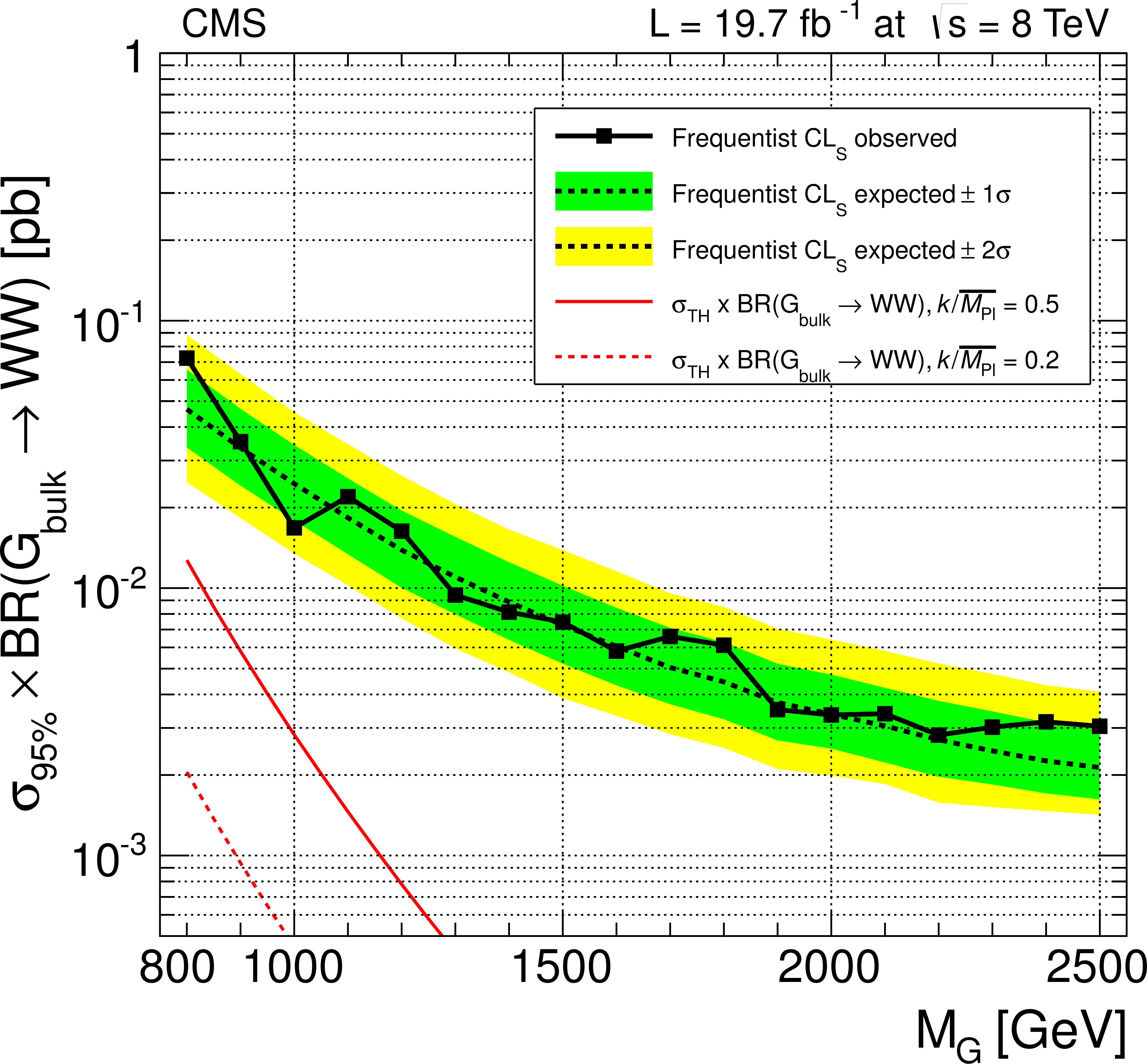
Figure 9-a:
Observed (solid) and expected (dashed) 95% CL upper limits on the product of the graviton production cross section and the branching fraction of $ { {\mathrm {G}} _{\mathrm {bulk}}}\to {\mathrm {W}} {\mathrm {W}}$ (a) and $ { {\mathrm {G}} _{\mathrm {bulk}}}\to {\mathrm {Z}} {\mathrm {Z}} $ (b). The cross section for the production of a bulk graviton multiplied by its branching fraction for the relevant process is shown as a red solid (dashed) curve for $ {k/\overline {M}_\mathrm {Pl}} =$ 0.5 (0.2), respectively. |

png pdf |
Figure 9-b:
Observed (solid) and expected (dashed) 95% CL upper limits on the product of the graviton production cross section and the branching fraction of $ { {\mathrm {G}} _{\mathrm {bulk}}}\to {\mathrm {W}} {\mathrm {W}}$ (a) and $ { {\mathrm {G}} _{\mathrm {bulk}}}\to {\mathrm {Z}} {\mathrm {Z}} $ (b). The cross section for the production of a bulk graviton multiplied by its branching fraction for the relevant process is shown as a red solid (dashed) curve for $ {k/\overline {M}_\mathrm {Pl}} =$ 0.5 (0.2), respectively. |
png pdf |
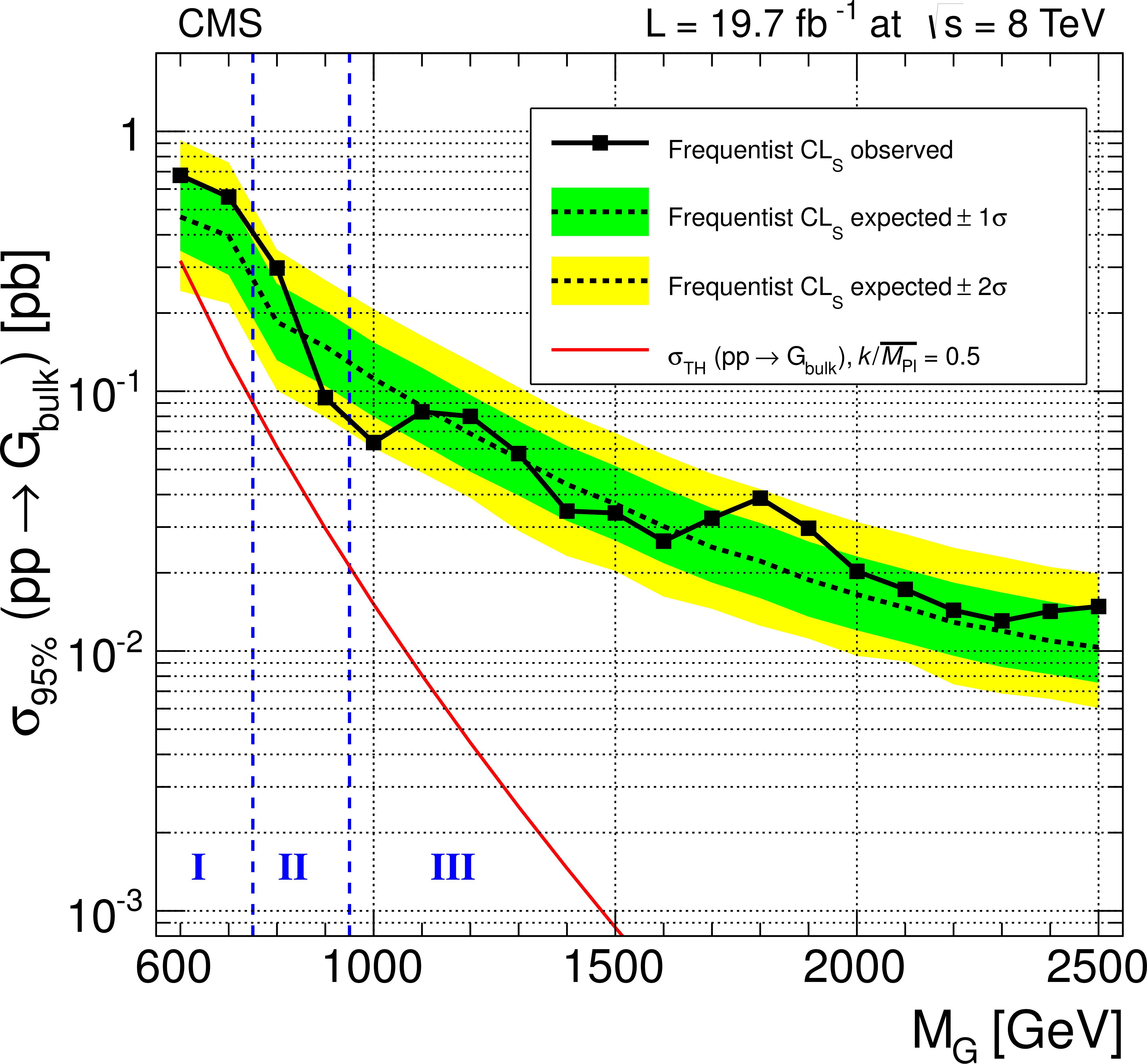
Figure 10-a:
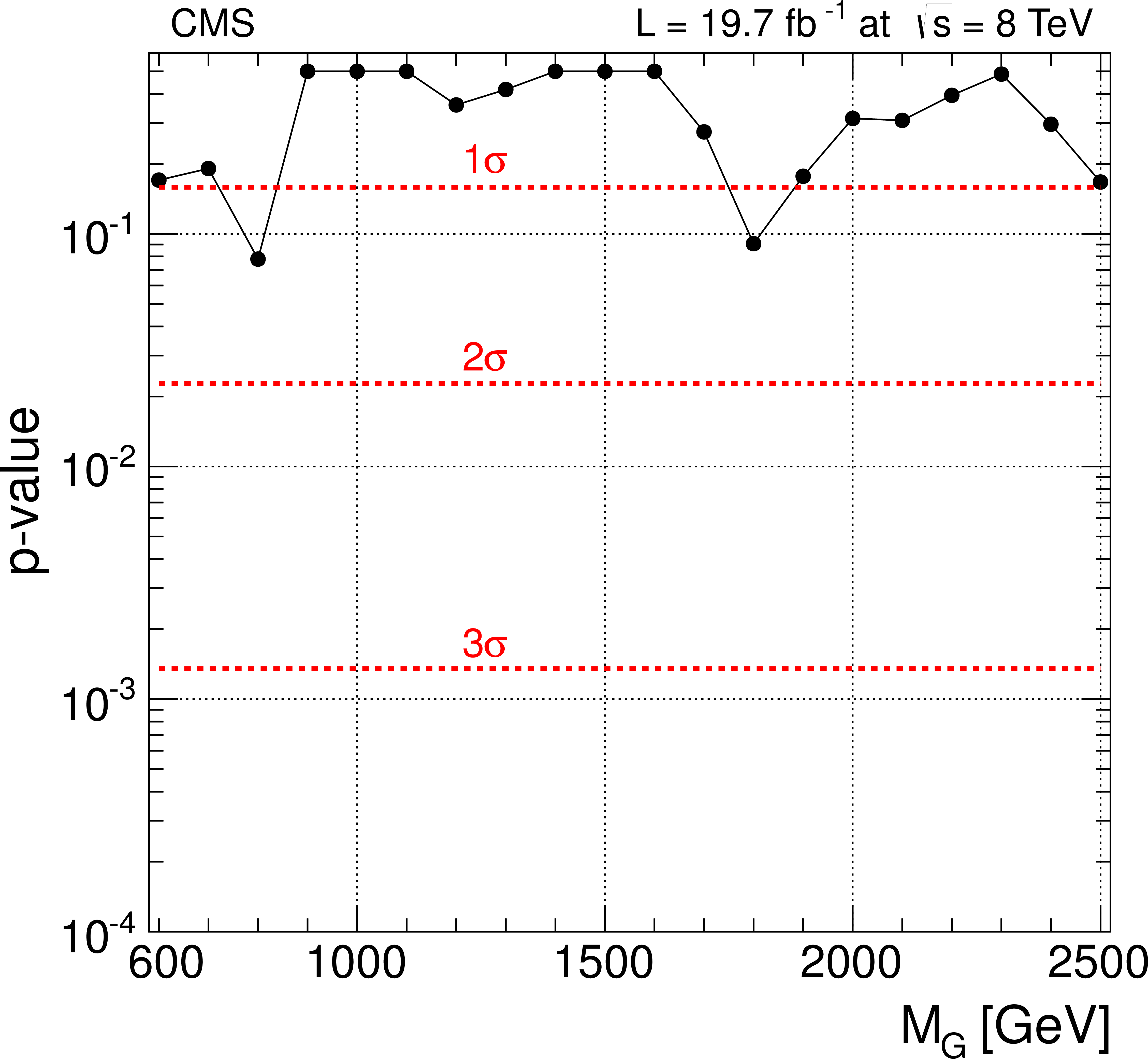
a: observed (solid) and expected (dashed) 95% CL upper limit on the graviton production cross section obtained with this analysis and the analysis of the all-hadronic channel. The cross section for the production of a bulk graviton with $ {k/\overline {M}_\mathrm {Pl}} =0.5$ is shown as a red solid curve. In region I, only the $ {\ell \ell }$+V-jet channel contributes. In region II, both $ {\ell \ell }$+V-jet and $ {\ell \nu }$+V-jet channels contribute. In region III, both the semi-leptonic and all-hadronic channels contribute. b: observed p-value as a function of the nominal signal mass. Conversions of the p-value to the number of standard deviations of a two-sided Gaussian distribution are drawn as dashed horizontal red lines. |
png pdf |
Figure 10-b:
a: observed (solid) and expected (dashed) 95% CL upper limit on the graviton production cross section obtained with this analysis and the analysis of the all-hadronic channel. The cross section for the production of a bulk graviton with $ {k/\overline {M}_\mathrm {Pl}} =0.5$ is shown as a red solid curve. In region I, only the $ {\ell \ell }$+V-jet channel contributes. In region II, both $ {\ell \ell }$+V-jet and $ {\ell \nu }$+V-jet channels contribute. In region III, both the semi-leptonic and all-hadronic channels contribute. b: observed p-value as a function of the nominal signal mass. Conversions of the p-value to the number of standard deviations of a two-sided Gaussian distribution are drawn as dashed horizontal red lines. |
png pdf |
Figure 11-a:
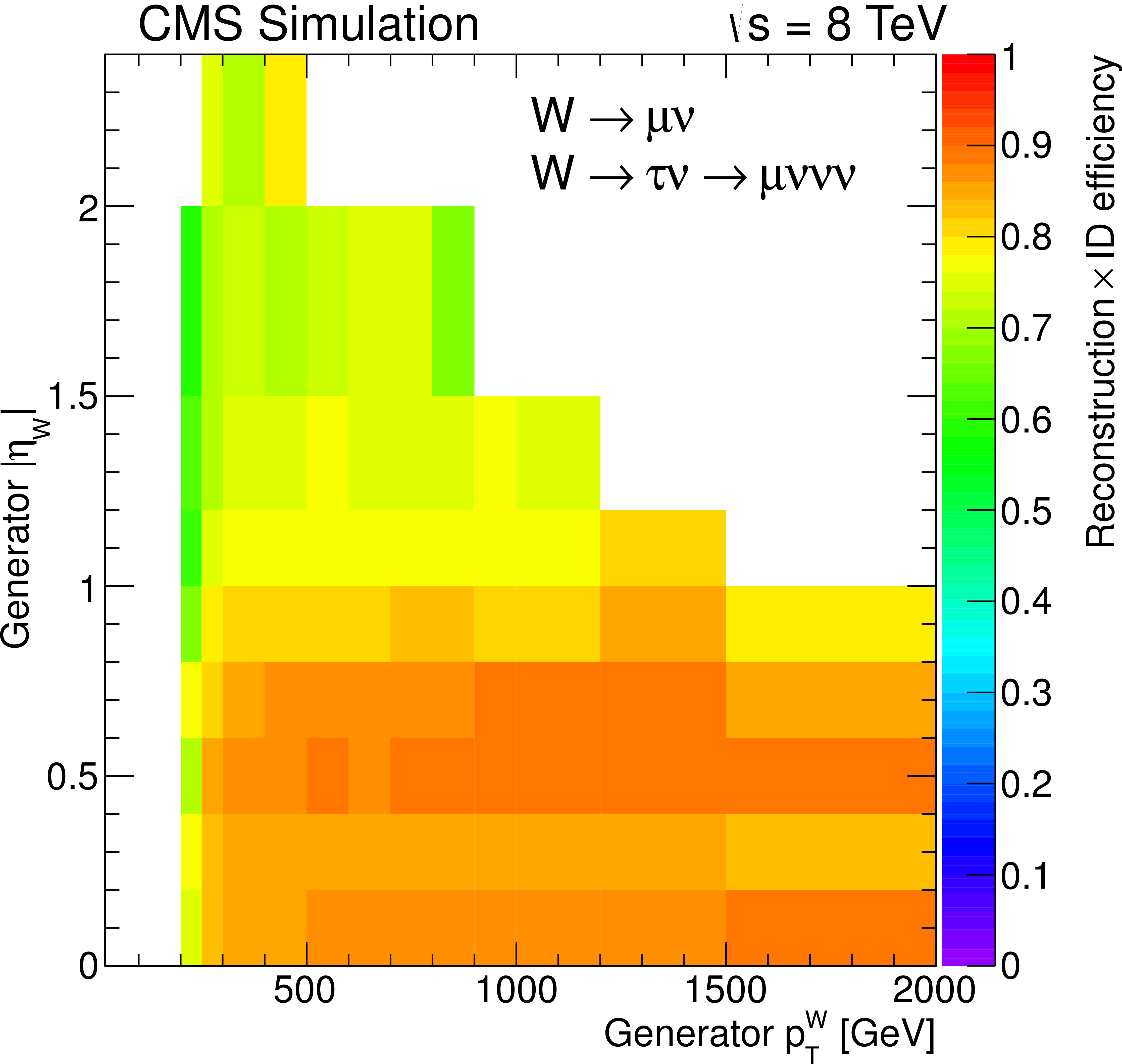
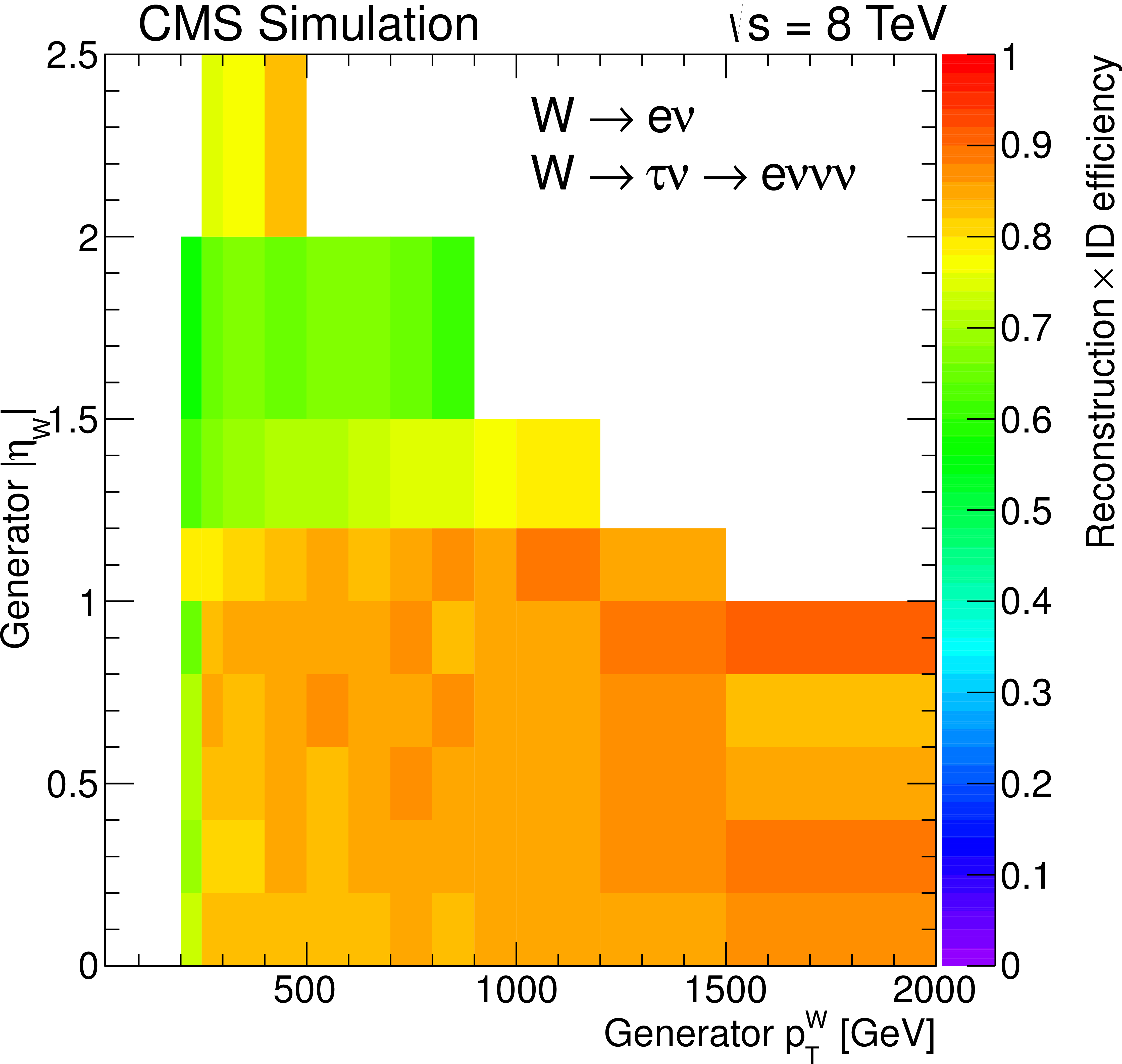
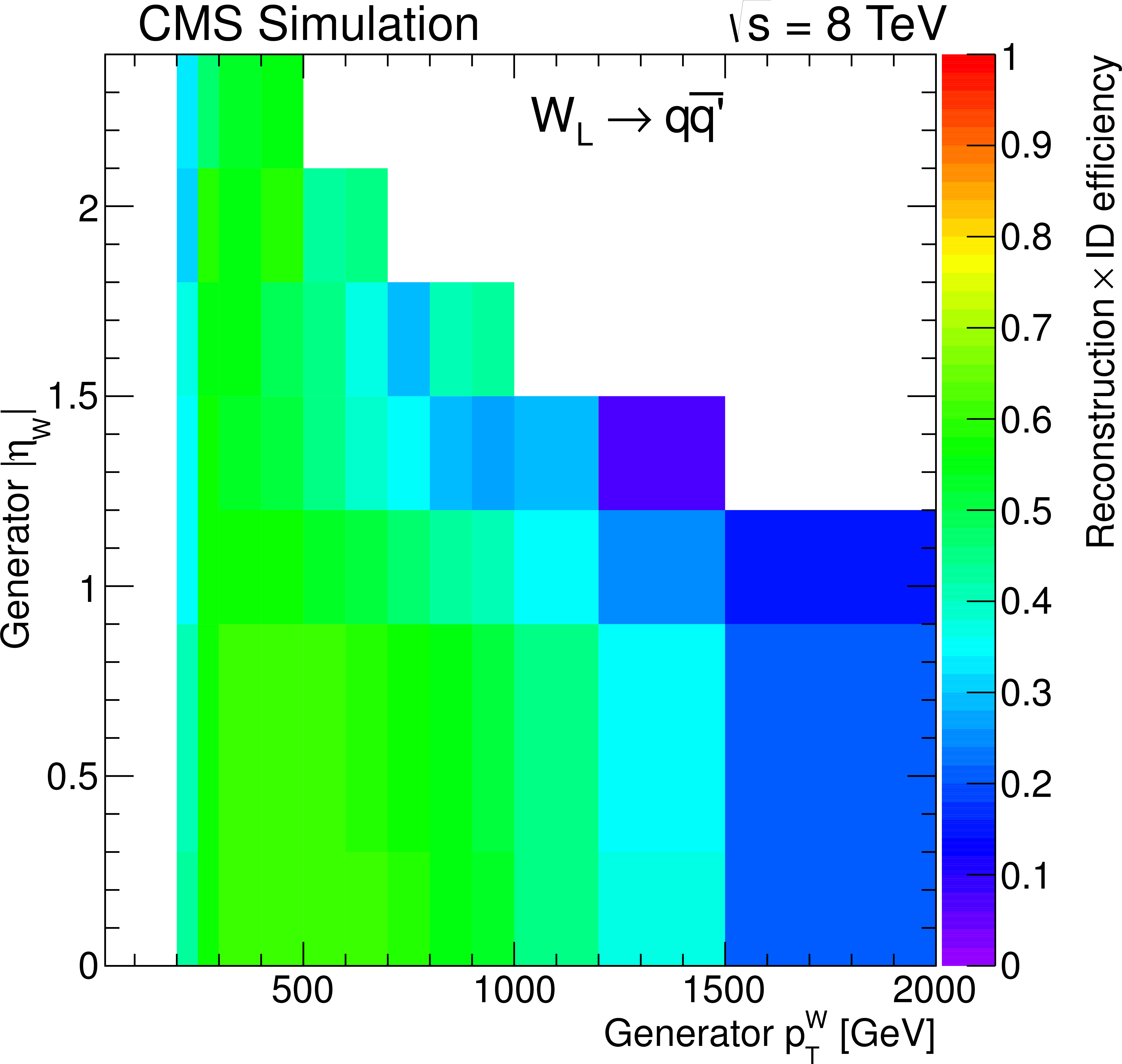
Reconstruction and identification efficiencies for the $ {\mathrm {W}}\to \mu \nu $ and $ {\mathrm {W}}\to \tau \nu \to \mu \nu \nu \nu $ (a), $ {\mathrm {W}}\to {\mathrm {e}}\nu $ and $ {\mathrm {W}}\to \tau \nu \to {\mathrm {e}}\nu \nu \nu $ (b), $ {\mathrm {W}}_\mathrm {L}\to {\mathrm {q}} {\mathrm {\overline {q}}}'$ (c), and $ {\mathrm {Z}}_\mathrm {L}\to {\mathrm {q}} {\mathrm {\overline {q}}}$ (d) decays as function of generated $ {p_{\mathrm {T}}} ^\mathrm {V}$ and $\eta _\mathrm {V}$ using the W-tagging requirements for the hadronic V decays. |
png pdf |
Figure 11-b:
Reconstruction and identification efficiencies for the $ {\mathrm {W}}\to \mu \nu $ and $ {\mathrm {W}}\to \tau \nu \to \mu \nu \nu \nu $ (a), $ {\mathrm {W}}\to {\mathrm {e}}\nu $ and $ {\mathrm {W}}\to \tau \nu \to {\mathrm {e}}\nu \nu \nu $ (b), $ {\mathrm {W}}_\mathrm {L}\to {\mathrm {q}} {\mathrm {\overline {q}}}'$ (c), and $ {\mathrm {Z}}_\mathrm {L}\to {\mathrm {q}} {\mathrm {\overline {q}}}$ (d) decays as function of generated $ {p_{\mathrm {T}}} ^\mathrm {V}$ and $\eta _\mathrm {V}$ using the W-tagging requirements for the hadronic V decays. |
png pdf |
Figure 11-c:
Reconstruction and identification efficiencies for the $ {\mathrm {W}}\to \mu \nu $ and $ {\mathrm {W}}\to \tau \nu \to \mu \nu \nu \nu $ (a), $ {\mathrm {W}}\to {\mathrm {e}}\nu $ and $ {\mathrm {W}}\to \tau \nu \to {\mathrm {e}}\nu \nu \nu $ (b), $ {\mathrm {W}}_\mathrm {L}\to {\mathrm {q}} {\mathrm {\overline {q}}}'$ (c), and $ {\mathrm {Z}}_\mathrm {L}\to {\mathrm {q}} {\mathrm {\overline {q}}}$ (d) decays as function of generated $ {p_{\mathrm {T}}} ^\mathrm {V}$ and $\eta _\mathrm {V}$ using the W-tagging requirements for the hadronic V decays. |
png pdf |
Figure 11-d:
Reconstruction and identification efficiencies for the $ {\mathrm {W}}\to \mu \nu $ and $ {\mathrm {W}}\to \tau \nu \to \mu \nu \nu \nu $ (a), $ {\mathrm {W}}\to {\mathrm {e}}\nu $ and $ {\mathrm {W}}\to \tau \nu \to {\mathrm {e}}\nu \nu \nu $ (b), $ {\mathrm {W}}_\mathrm {L}\to {\mathrm {q}} {\mathrm {\overline {q}}}'$ (c), and $ {\mathrm {Z}}_\mathrm {L}\to {\mathrm {q}} {\mathrm {\overline {q}}}$ (d) decays as function of generated $ {p_{\mathrm {T}}} ^\mathrm {V}$ and $\eta _\mathrm {V}$ using the W-tagging requirements for the hadronic V decays. |
png pdf |
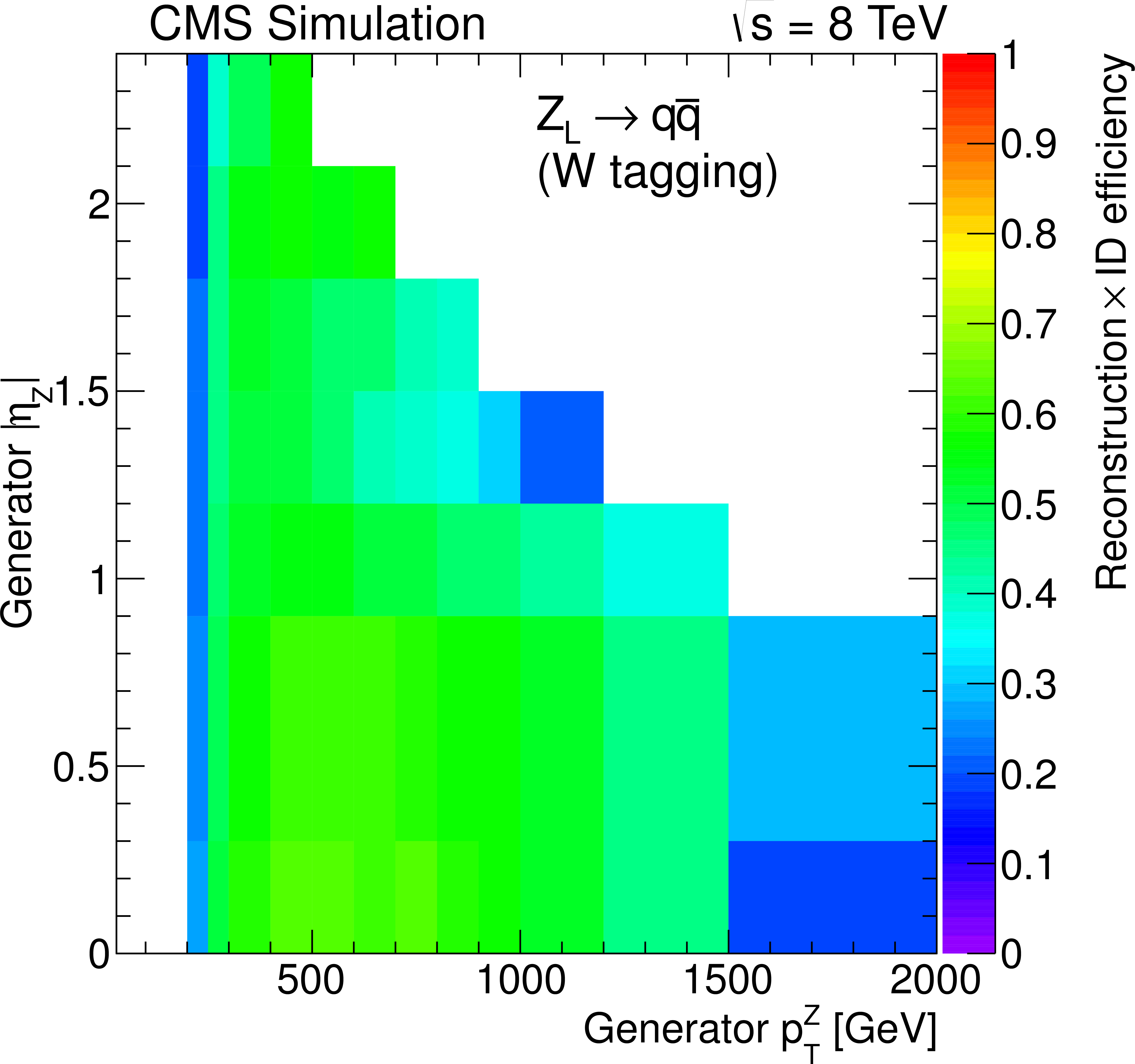
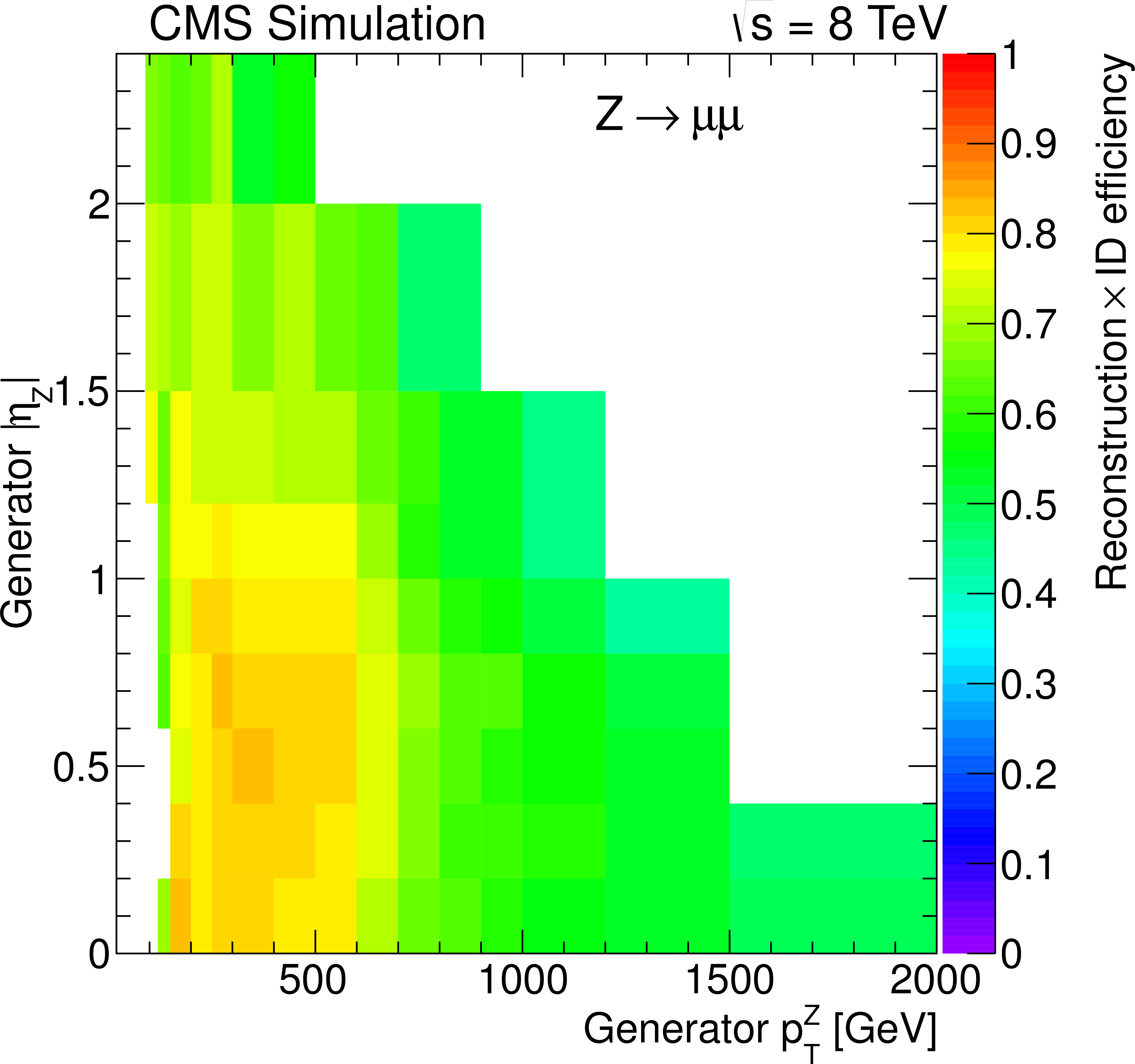
Figure 12-a:
Reconstruction and identification efficiencies for the $ {\mathrm {Z}} \to \mu \mu $ (a), $ {\mathrm {Z}} \to {\mathrm {e}} {\mathrm {e}}$ (b), $ {\mathrm {Z}} _{\text {L}}\to {\mathrm {q}} {\mathrm {\overline {q}}}$ (c), and $ {\mathrm {W}}_\mathrm {L}\to {\mathrm {q}} {\mathrm {\overline {q}}}'$ (d) decays as a function of generated $ {p_{\mathrm {T}}} ^\mathrm {V}$ and $\eta _\mathrm {V}$ using the Z-tagging requirements for the hadronic V decays. |

png pdf |
Figure 12-b:
Reconstruction and identification efficiencies for the $ {\mathrm {Z}} \to \mu \mu $ (a), $ {\mathrm {Z}} \to {\mathrm {e}} {\mathrm {e}}$ (b), $ {\mathrm {Z}} _{\text {L}}\to {\mathrm {q}} {\mathrm {\overline {q}}}$ (c), and $ {\mathrm {W}}_\mathrm {L}\to {\mathrm {q}} {\mathrm {\overline {q}}}'$ (d) decays as a function of generated $ {p_{\mathrm {T}}} ^\mathrm {V}$ and $\eta _\mathrm {V}$ using the Z-tagging requirements for the hadronic V decays. |

png pdf |
Figure 12-c:
Reconstruction and identification efficiencies for the $ {\mathrm {Z}} \to \mu \mu $ (a), $ {\mathrm {Z}} \to {\mathrm {e}} {\mathrm {e}}$ (b), $ {\mathrm {Z}} _{\text {L}}\to {\mathrm {q}} {\mathrm {\overline {q}}}$ (c), and $ {\mathrm {W}}_\mathrm {L}\to {\mathrm {q}} {\mathrm {\overline {q}}}'$ (d) decays as a function of generated $ {p_{\mathrm {T}}} ^\mathrm {V}$ and $\eta _\mathrm {V}$ using the Z-tagging requirements for the hadronic V decays. |

png pdf |
Figure 12-d:
Reconstruction and identification efficiencies for the $ {\mathrm {Z}} \to \mu \mu $ (a), $ {\mathrm {Z}} \to {\mathrm {e}} {\mathrm {e}}$ (b), $ {\mathrm {Z}} _{\text {L}}\to {\mathrm {q}} {\mathrm {\overline {q}}}$ (c), and $ {\mathrm {W}}_\mathrm {L}\to {\mathrm {q}} {\mathrm {\overline {q}}}'$ (d) decays as a function of generated $ {p_{\mathrm {T}}} ^\mathrm {V}$ and $\eta _\mathrm {V}$ using the Z-tagging requirements for the hadronic V decays. |
png pdf |
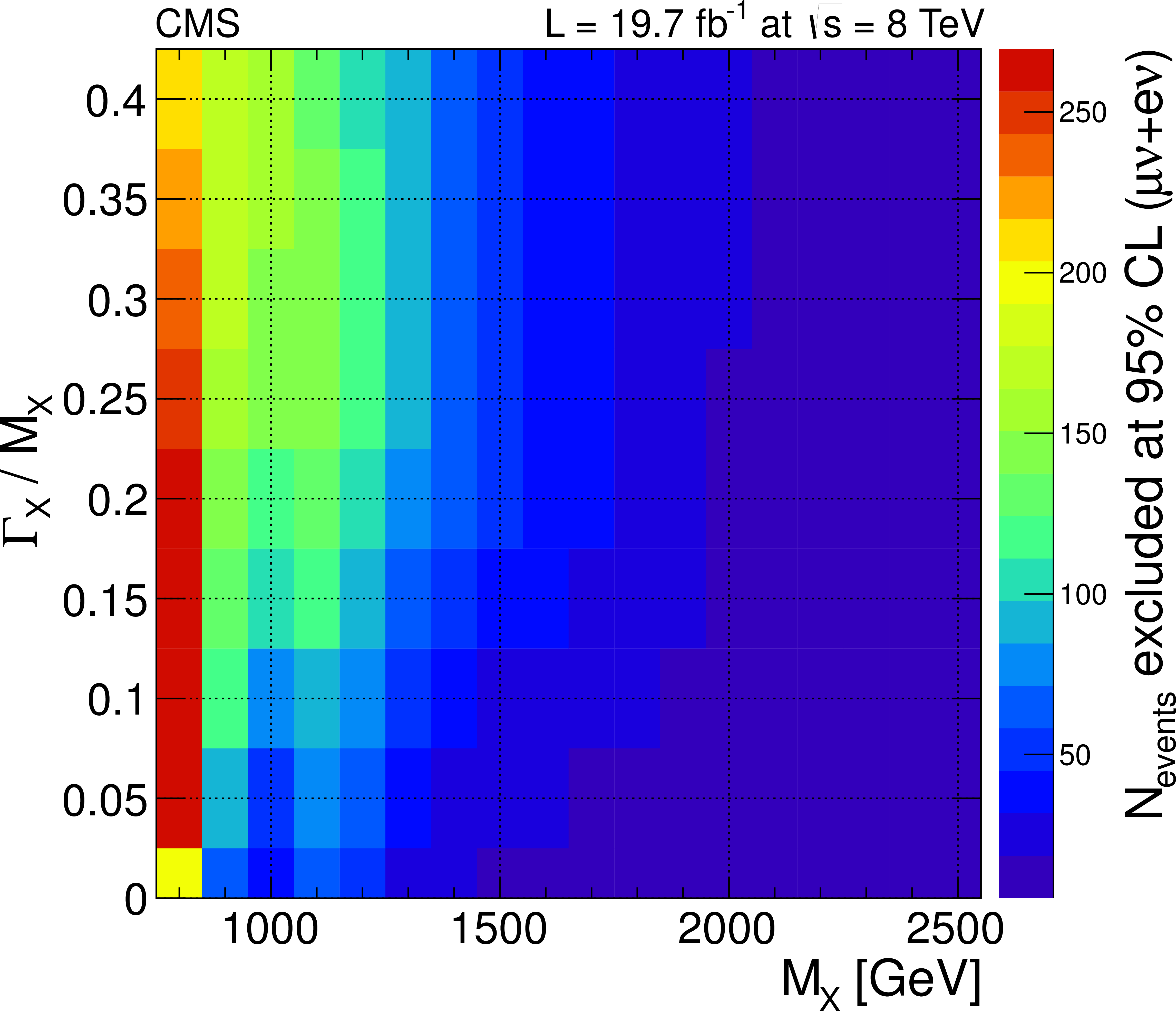
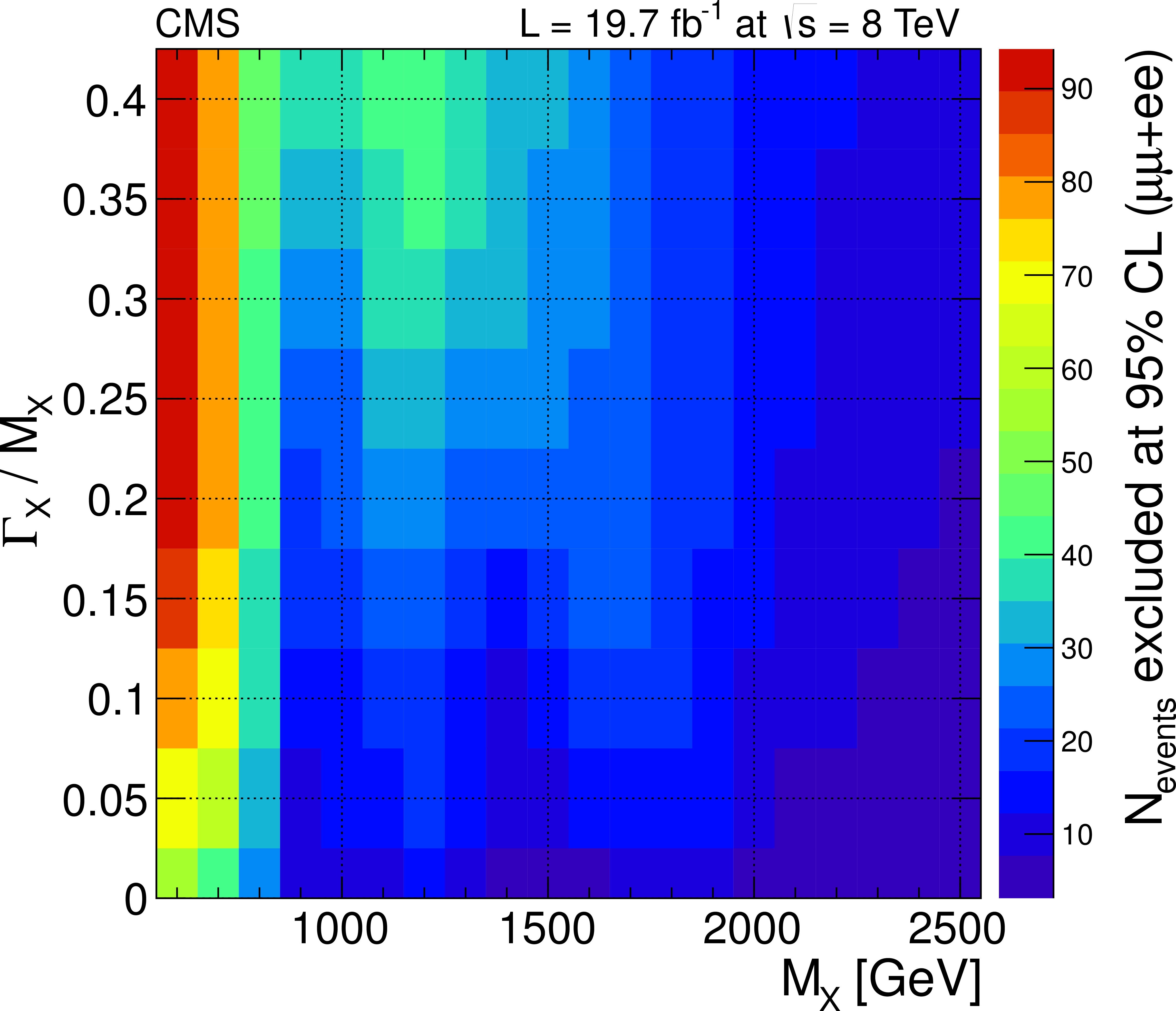
Figure 13-a:
Observed exclusion limits at 95% CL on the number of events for a $ {\mathrm {W}} {\mathrm {V}} \to {\ell \nu }+V-jet $ (a) and a $ {\mathrm {Z}} {\mathrm {V}} \to {\ell \ell }+V-jet $ (b) resonance, as a function of its mass and normalized width. |
png pdf |
Figure 13-b:
Observed exclusion limits at 95% CL on the number of events for a $ {\mathrm {W}} {\mathrm {V}} \to {\ell \nu }+V-jet $ (a) and a $ {\mathrm {Z}} {\mathrm {V}} \to {\ell \ell }+V-jet $ (b) resonance, as a function of its mass and normalized width. |
| Summary |
| We have presented a search for new resonances decaying to WW, ZZ, or WZ in which one of the bosons decays leptonically and the other hadronically. The final states considered are either $\ell \nu \mathrm{qq(^{\prime})}$ or $\ell \ell \mathrm{qq(^{\prime})}$ with $\ell = \mu$ or e. The results include the case in which W $\to \tau \nu$ or Z $\to \tau \tau $ where the tau decay is $\tau \to \ell \nu\nu$. The events are reconstructed as a leptonic W or Z candidate recoiling against a jet with mass compatible with the W or Z mass, respectively. Additional information from jet substructure is used to reduce the background from multijet processes. No evidence for a signal is found, and the result is interpreted as an upper limit on the production cross section as a function of the resonance mass in the context of the bulk graviton model. The final upper limits are based on the statistical combination of the two semi-leptonic channels considered here with those of a complementary search in the fully-hadronic final state. Upper limits at 95% CL are set on the bulk graviton production cross section in the range from 700 to 10 fb for resonance masses between 600 and 2500 GeV, respectively. These limits are the most stringent to date in these final states. The two analyses in the semi-leptonic channels are repeated in a simplified scenario, providing model-independent limits on the number of events. The tabulated efficiency of reconstructing the vector bosons within the kinematic acceptance of the analysis allows the reinterpretation of the exclusion limits in a generic phenomenological model, including WZ resonances, greatly extending the versatility of these results. |
|
|
Compact Muon Solenoid LHC, CERN |
|

|

|

|

|

|