

Compact Muon Solenoid
LHC, CERN
| CMS-EXO-14-014 ; CERN-EP-2016-032 | ||
| Search for heavy Majorana neutrinos in $\mathrm{ e^\pm e^\pm }$+ jets and $\mathrm{ e^\pm \mu^\pm }$+ jets events in proton-proton collisions at $\sqrt{s} =$ 8 TeV | ||
| CMS Collaboration | ||
| 7 March 2016 | ||
| JHEP 04 (2016) 169 | ||
| Abstract: A search is performed for heavy Majorana neutrinos (N) decaying into a W boson and a lepton using the CMS detector at the Large Hadron Collider. A signature of two jets and either two same sign electrons or a same sign electron-muon pair is searched for using 19.7 fb$^{-1}$ of data collected during 2012 in proton-proton collisions at a centre-of-mass energy of 8 TeV. The data are found to be consistent with the expected standard model (SM) background and, in the context of a Type-1 seesaw mechanism, upper limits are set on the cross section times branching fraction for production of heavy Majorana neutrinos in the mass range between 40 and 500 GeV. The results are additionally interpreted as limits on the mixing between the heavy Majorana neutrinos and the SM neutrinos. In the mass range considered, the upper limits range between 0.00015-0.72 for $| \mathrm{V_{eN}} |^2$ and 6.6 $\times$ 10$^{-5}$-0.47 for $| \mathrm{ V^{ }_{eN} } \mathrm{V^{*}_{\mu N}} |^2 / ( | \mathrm{V_{eN}} |^2 + | \mathrm{V_{\mu N}} |^2 )$, where $ \mathrm{V_{\ell N}} $ is the mixing element describing the mixing of the heavy neutrino with the SM neutrino of flavour $\ell$. These limits are the most restrictive direct limits for heavy Majorana neutrino masses above 200 GeV. | ||
| Links: e-print arXiv:1603.02248 [hep-ex] (PDF) ; CDS record ; inSPIRE record ; HepData record ; CADI line (restricted) ; | ||
| Figures | |
png pdf |
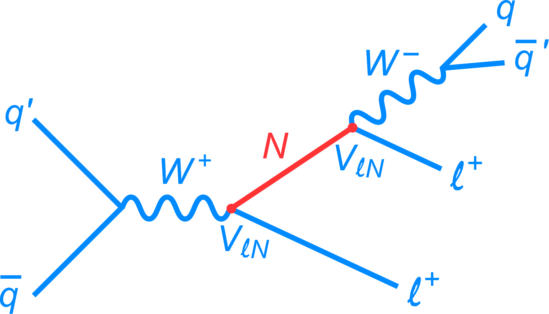
Figure 1:
The Feynman diagram for resonant production of a Majorana neutrino (N). The charge-conjugate diagram results in a $\ell ^- \ell ^- \mathrm{ \bar{q} q' } $ final state. |

png pdf |
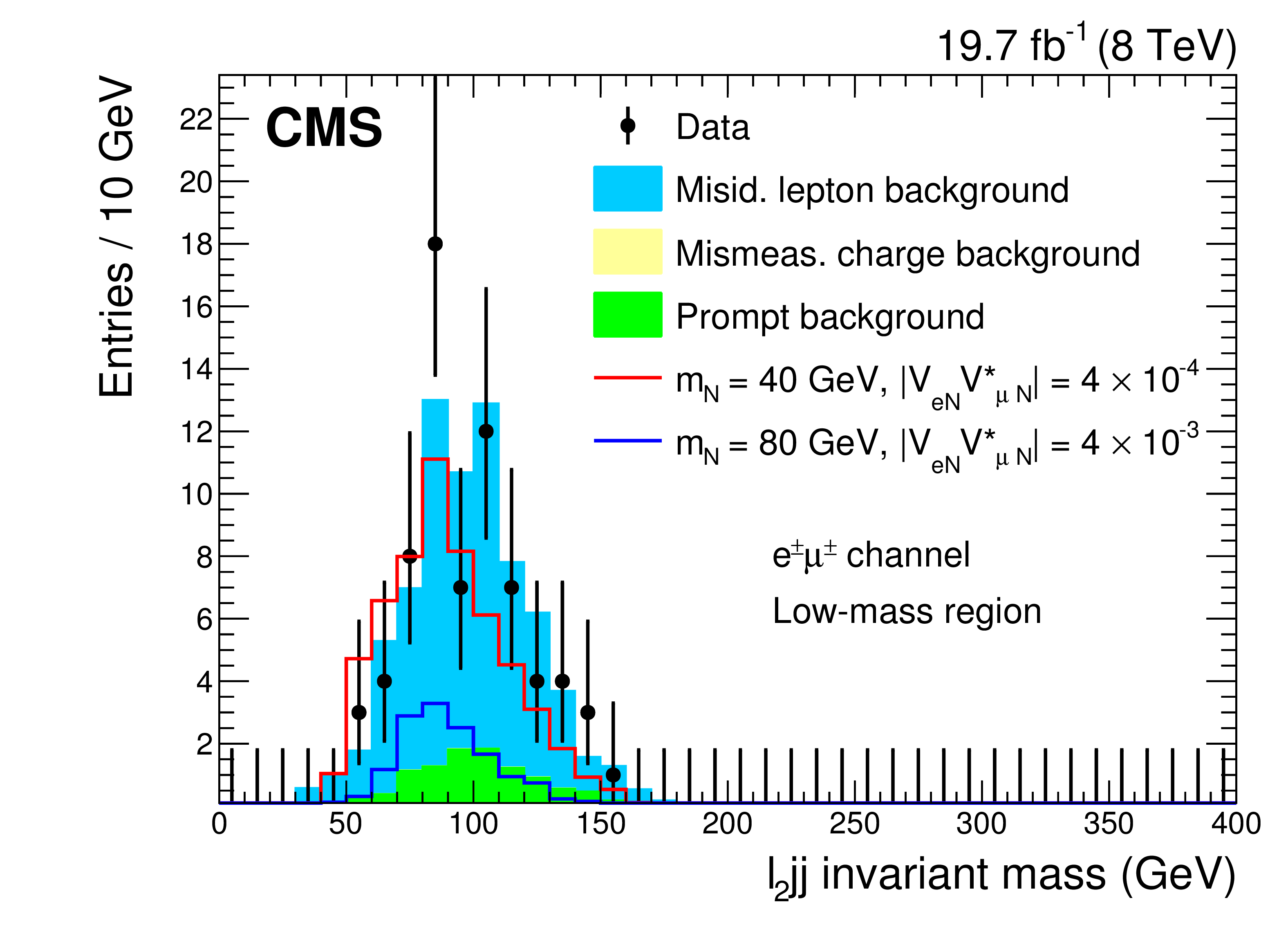
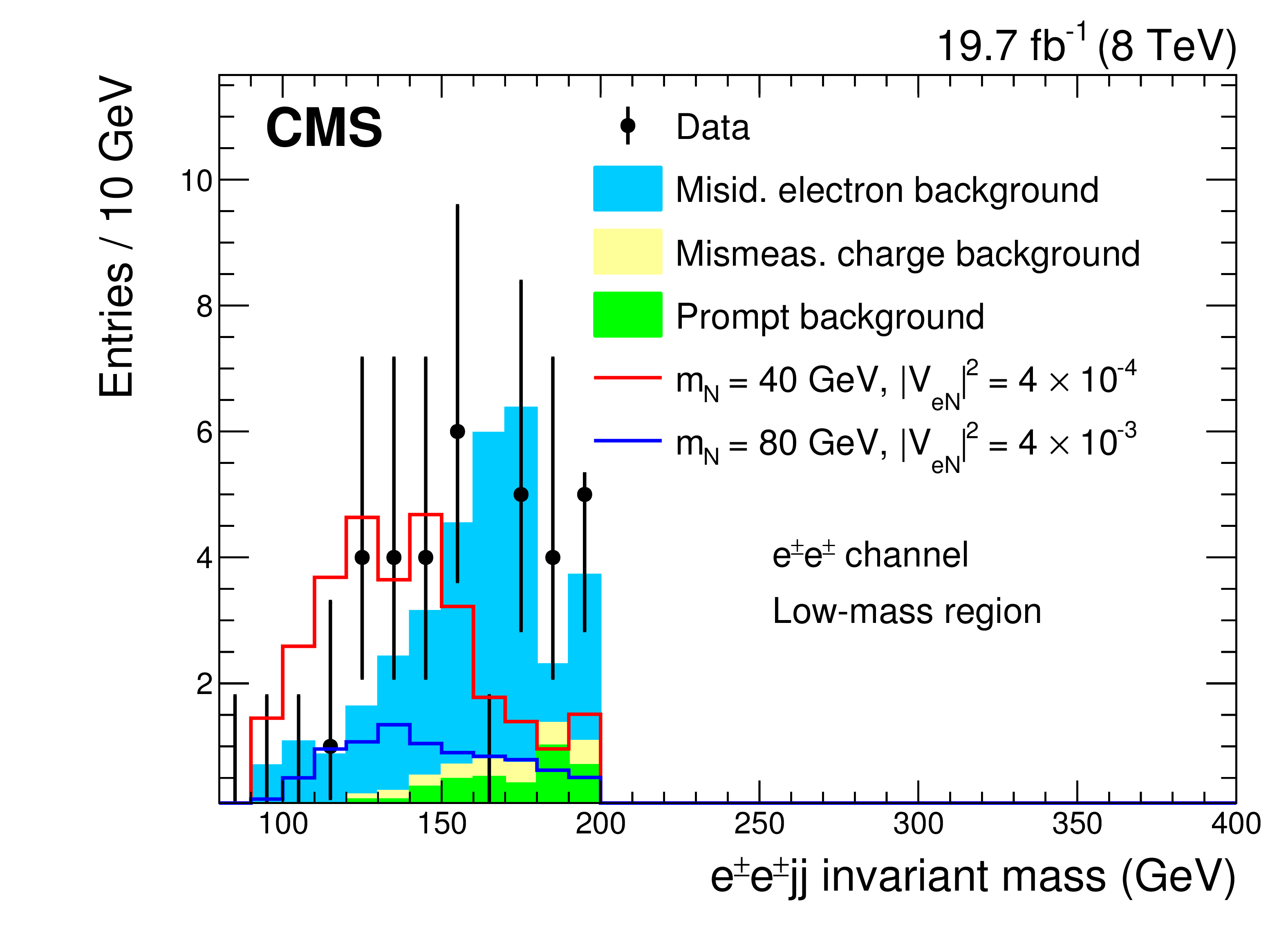
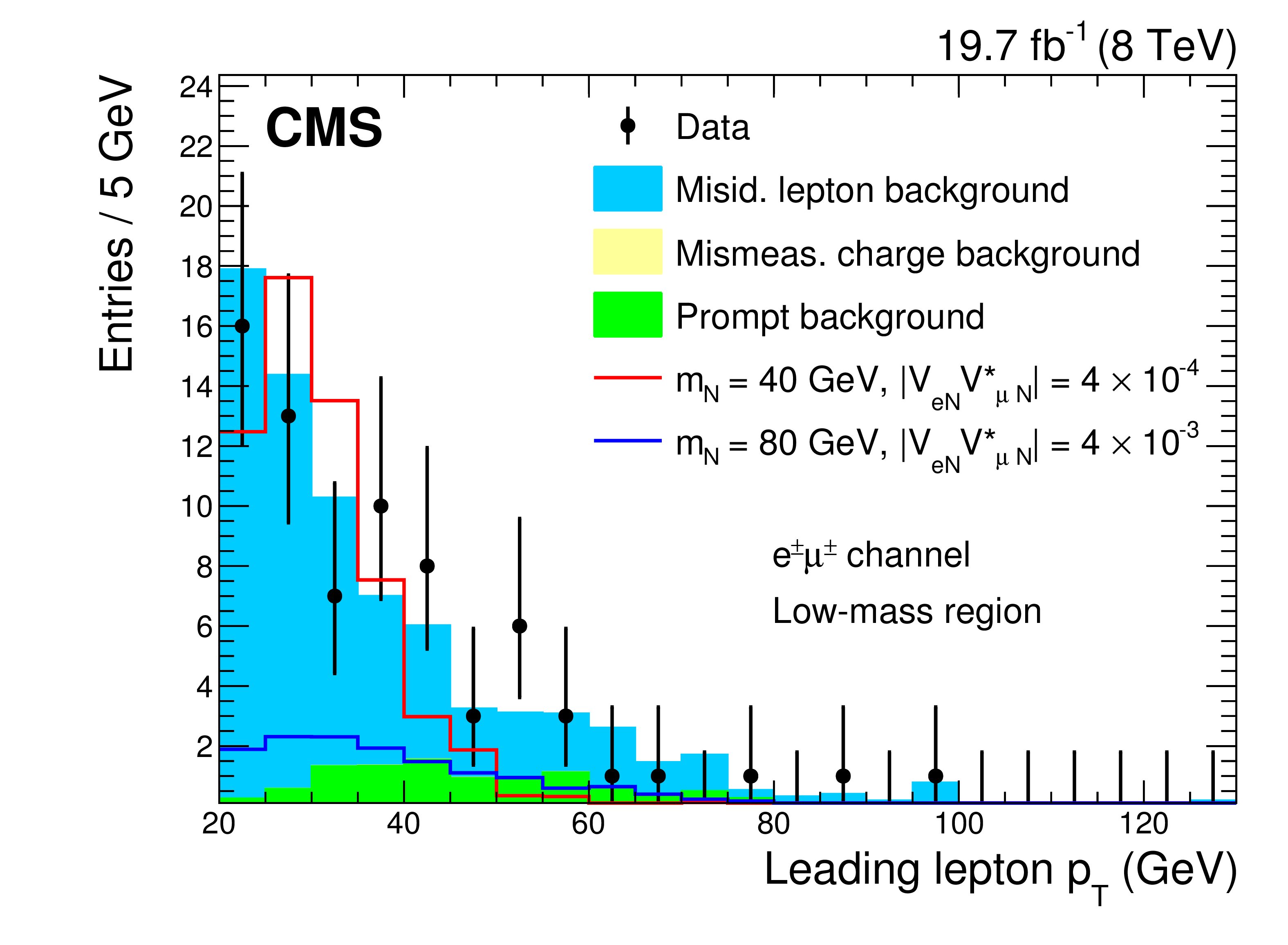
Figure 2-a:
Kinematic distributions for the low-mass region after all selection cuts are applied except for the final optimization requirement: dielectron channel (a), electron-muon channel (b). The plots show the data, backgrounds, and two choices for the heavy Majorana neutrino signal. |
png pdf |
Figure 2-b:
Kinematic distributions for the low-mass region after all selection cuts are applied except for the final optimization requirement: dielectron channel (a), electron-muon channel (b). The plots show the data, backgrounds, and two choices for the heavy Majorana neutrino signal. |
png pdf |
Figure 2-c:
Kinematic distributions for the low-mass region after all selection cuts are applied except for the final optimization requirement: dielectron channel (a), electron-muon channel (b). The plots show the data, backgrounds, and two choices for the heavy Majorana neutrino signal. |

png pdf |
Figure 2-d:
Kinematic distributions for the low-mass region after all selection cuts are applied except for the final optimization requirement: dielectron channel (a), electron-muon channel (b). The plots show the data, backgrounds, and two choices for the heavy Majorana neutrino signal. |

png pdf |
Figure 2-e:
Kinematic distributions for the low-mass region after all selection cuts are applied except for the final optimization requirement: dielectron channel (a), electron-muon channel (b). The plots show the data, backgrounds, and two choices for the heavy Majorana neutrino signal. |
png pdf |
Figure 2-f:
Kinematic distributions for the low-mass region after all selection cuts are applied except for the final optimization requirement: dielectron channel (a), electron-muon channel (b). The plots show the data, backgrounds, and two choices for the heavy Majorana neutrino signal. |
png pdf |
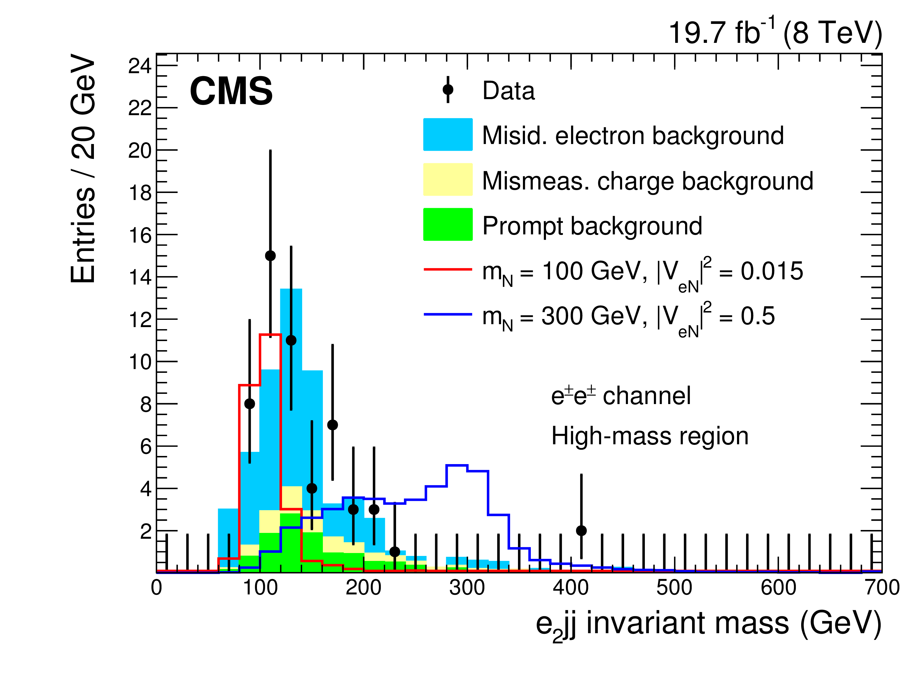
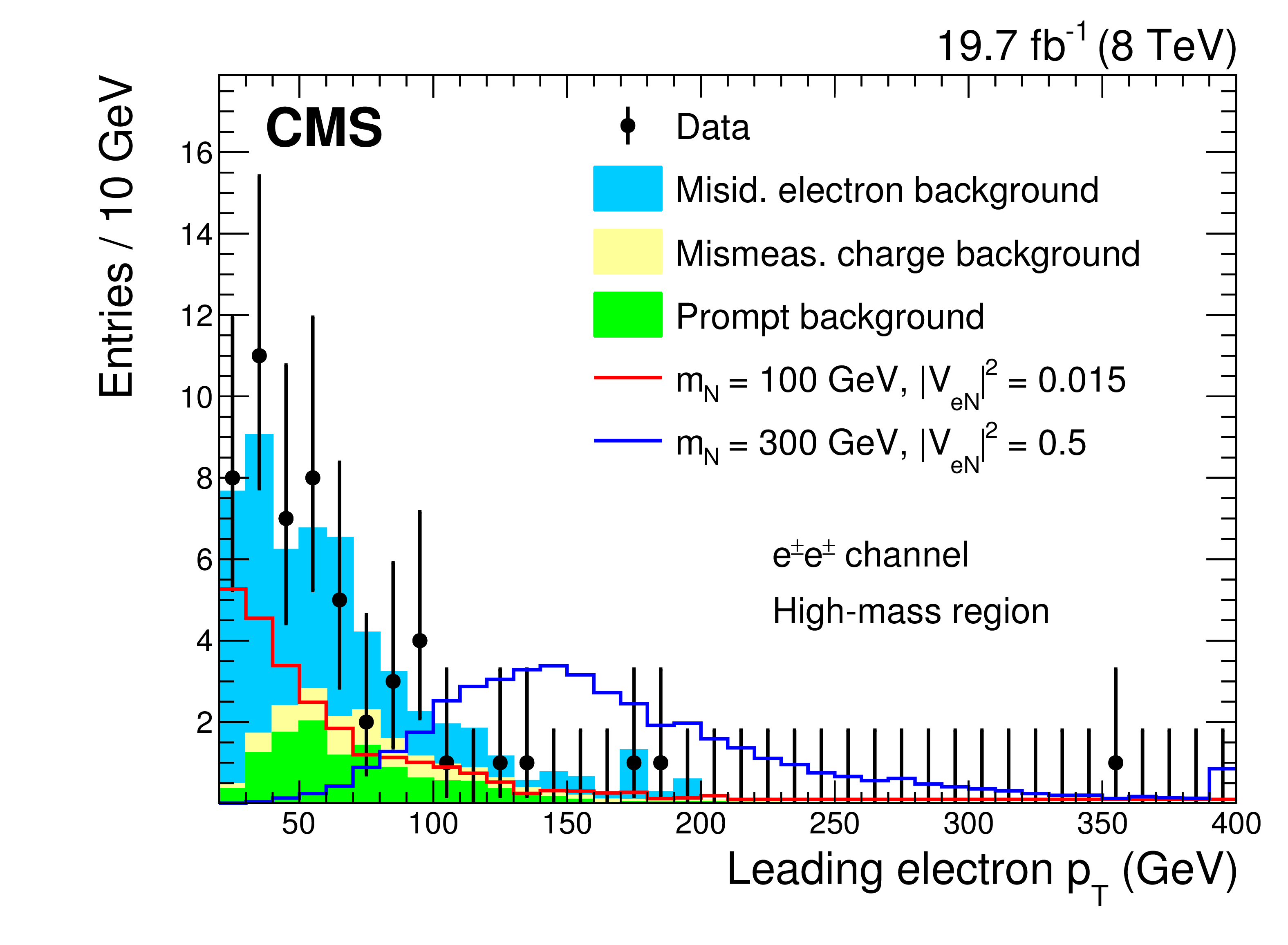
Figure 3-a:
Kinematic distributions for the high-mass region after all selection cuts are applied except for the final optimization requirement: dielectron channel (a), electron-muon channel (b). The plots show the data, backgrounds, and two choices for the heavy Majorana neutrino signal. |
png pdf |
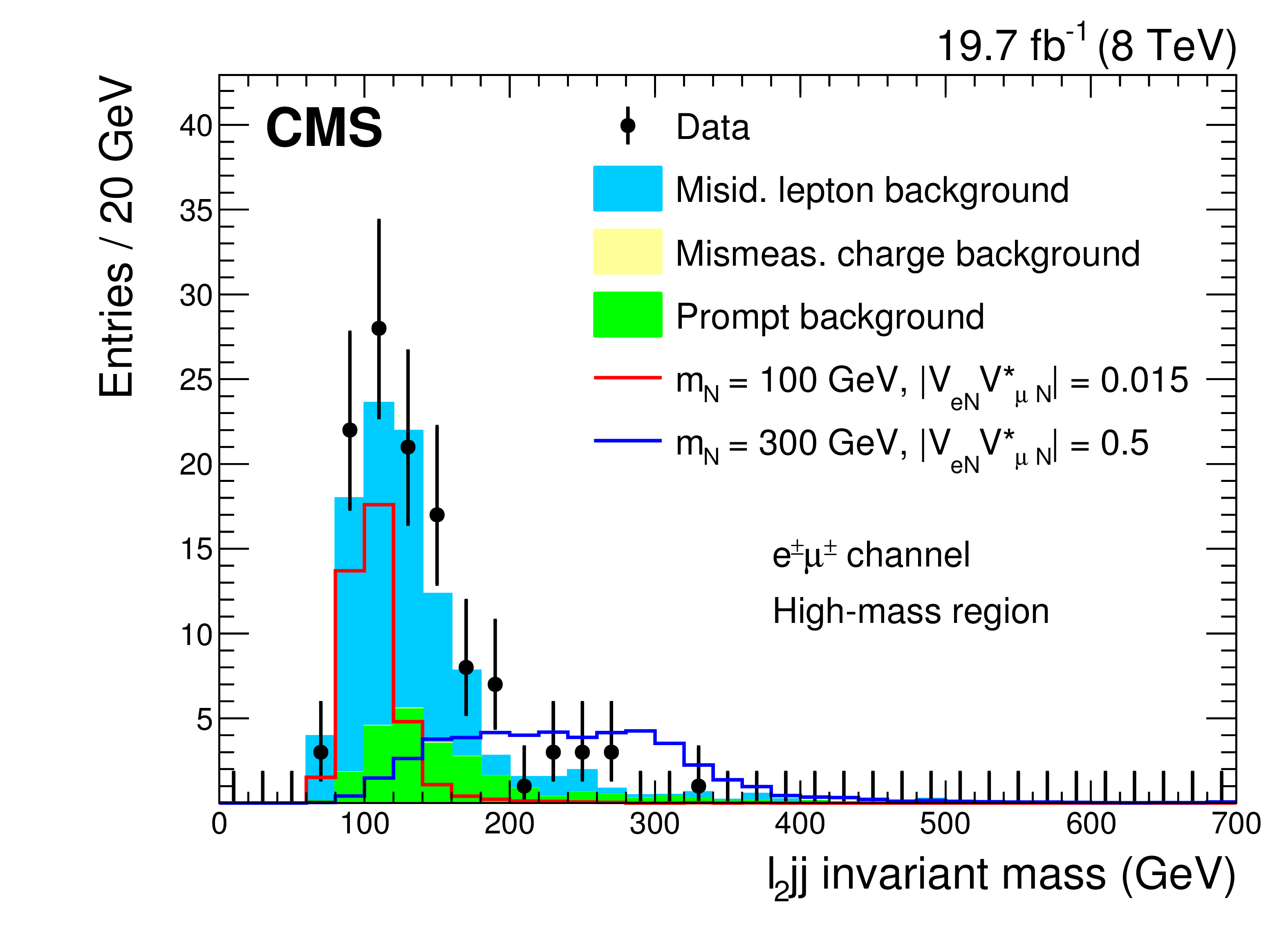
Figure 3-b:
Kinematic distributions for the high-mass region after all selection cuts are applied except for the final optimization requirement: dielectron channel (a), electron-muon channel (b). The plots show the data, backgrounds, and two choices for the heavy Majorana neutrino signal. |
png pdf |
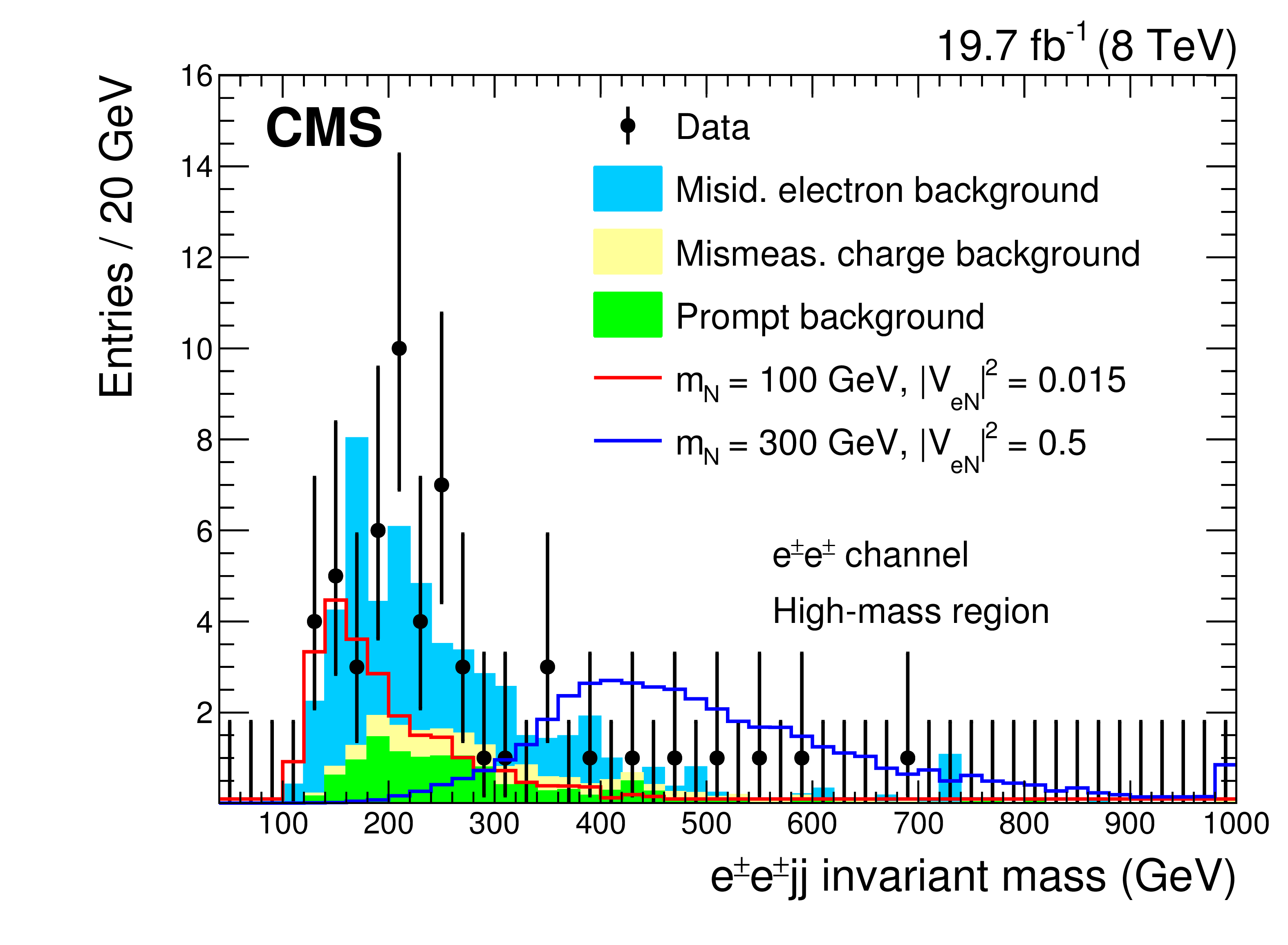
Figure 3-c:
Kinematic distributions for the high-mass region after all selection cuts are applied except for the final optimization requirement: dielectron channel (a), electron-muon channel (b). The plots show the data, backgrounds, and two choices for the heavy Majorana neutrino signal. |
png pdf |
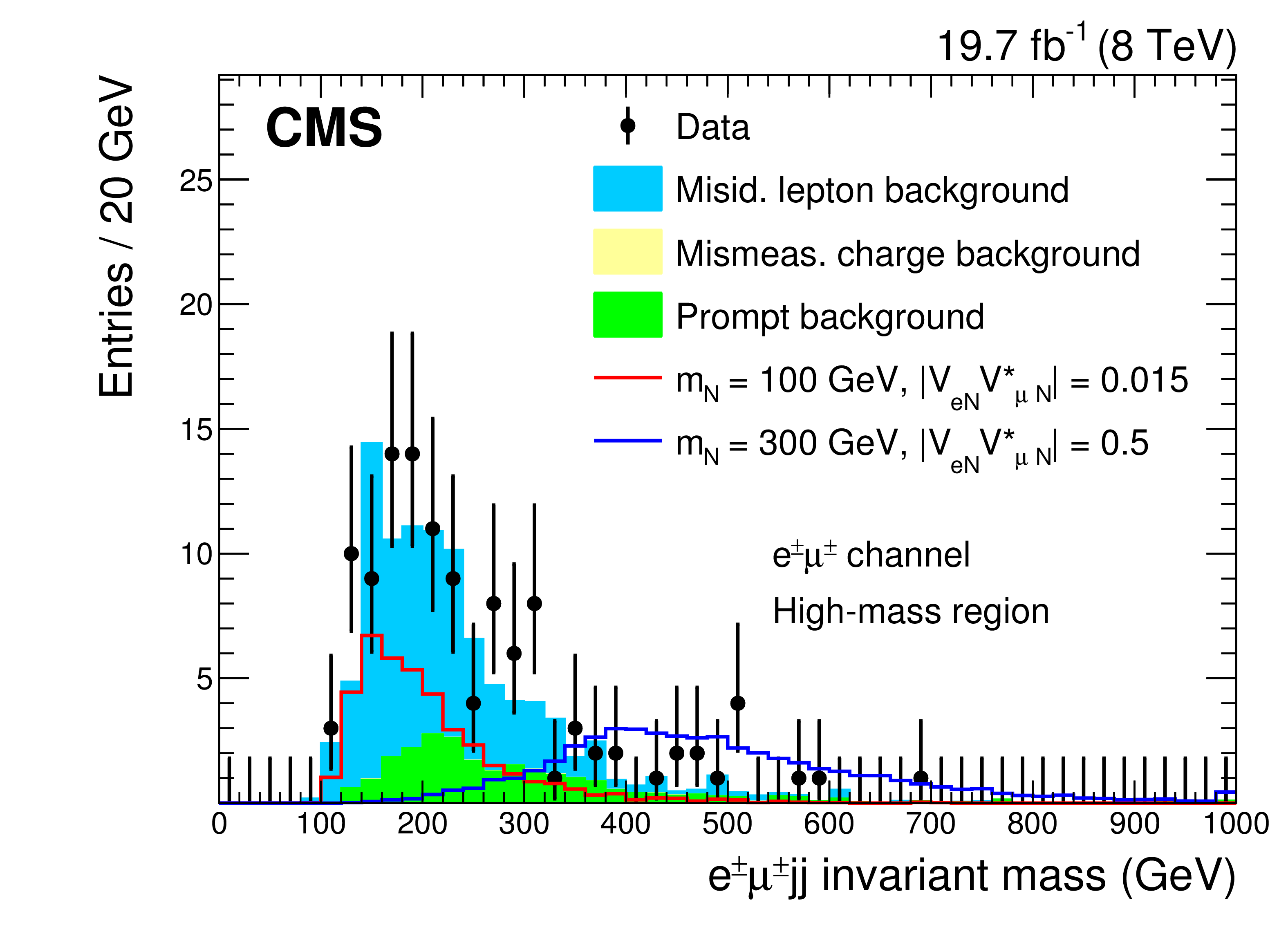
Figure 3-d:
Kinematic distributions for the high-mass region after all selection cuts are applied except for the final optimization requirement: dielectron channel (a), electron-muon channel (b). The plots show the data, backgrounds, and two choices for the heavy Majorana neutrino signal. |
png pdf |
Figure 3-e:
Kinematic distributions for the high-mass region after all selection cuts are applied except for the final optimization requirement: dielectron channel (a), electron-muon channel (b). The plots show the data, backgrounds, and two choices for the heavy Majorana neutrino signal. |

png pdf |
Figure 3-f:
Kinematic distributions for the high-mass region after all selection cuts are applied except for the final optimization requirement: dielectron channel (a), electron-muon channel (b). The plots show the data, backgrounds, and two choices for the heavy Majorana neutrino signal. |
png pdf |
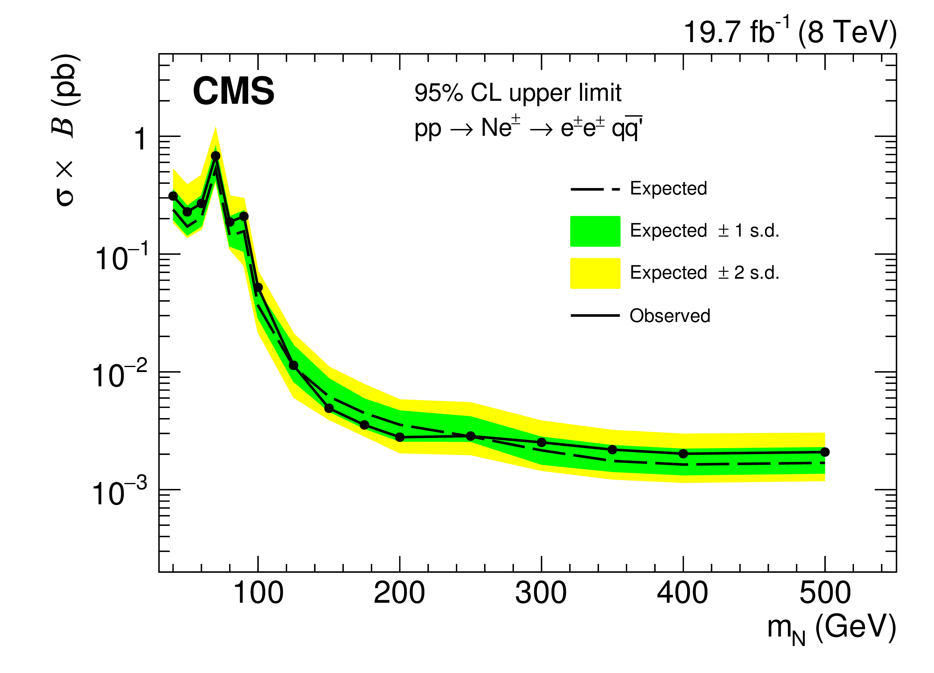
Figure 4-a:
Exclusion region at 95% CL in the cross section times branching fraction for $\sigma ( {\mathrm { pp }} \rightarrow {\mathrm {N}} {\mathrm { e }} ^{\pm } \rightarrow {\mathrm { e }} ^\pm {\mathrm { e }} ^\pm {\mathrm { q }} {\mathrm { \bar{q} }} ^\prime )$ (a) and $\sigma ( {\mathrm { pp }} \rightarrow {\mathrm {N}} \, {\mathrm { e }} ^{\pm } / \mu ^\pm \rightarrow {\mathrm { e }} ^\pm \mu ^\pm {\mathrm { q }} {\mathrm { \bar{q} }} ^\prime )$ (b) as a function of $ {m_{ {\mathrm {N}} }} $. The dashed curve is the expected upper limit, with one and two standard-deviation bands shown in dark green and light yellow, respectively. The solid black curve is the observed upper limit. |

png pdf |
Figure 4-b:
Exclusion region at 95% CL in the cross section times branching fraction for $\sigma ( {\mathrm { pp }} \rightarrow {\mathrm {N}} {\mathrm { e }} ^{\pm } \rightarrow {\mathrm { e }} ^\pm {\mathrm { e }} ^\pm {\mathrm { q }} {\mathrm { \bar{q} }} ^\prime )$ (a) and $\sigma ( {\mathrm { pp }} \rightarrow {\mathrm {N}} \, {\mathrm { e }} ^{\pm } / \mu ^\pm \rightarrow {\mathrm { e }} ^\pm \mu ^\pm {\mathrm { q }} {\mathrm { \bar{q} }} ^\prime )$ (b) as a function of $ {m_{ {\mathrm {N}} }} $. The dashed curve is the expected upper limit, with one and two standard-deviation bands shown in dark green and light yellow, respectively. The solid black curve is the observed upper limit. |
png pdf |
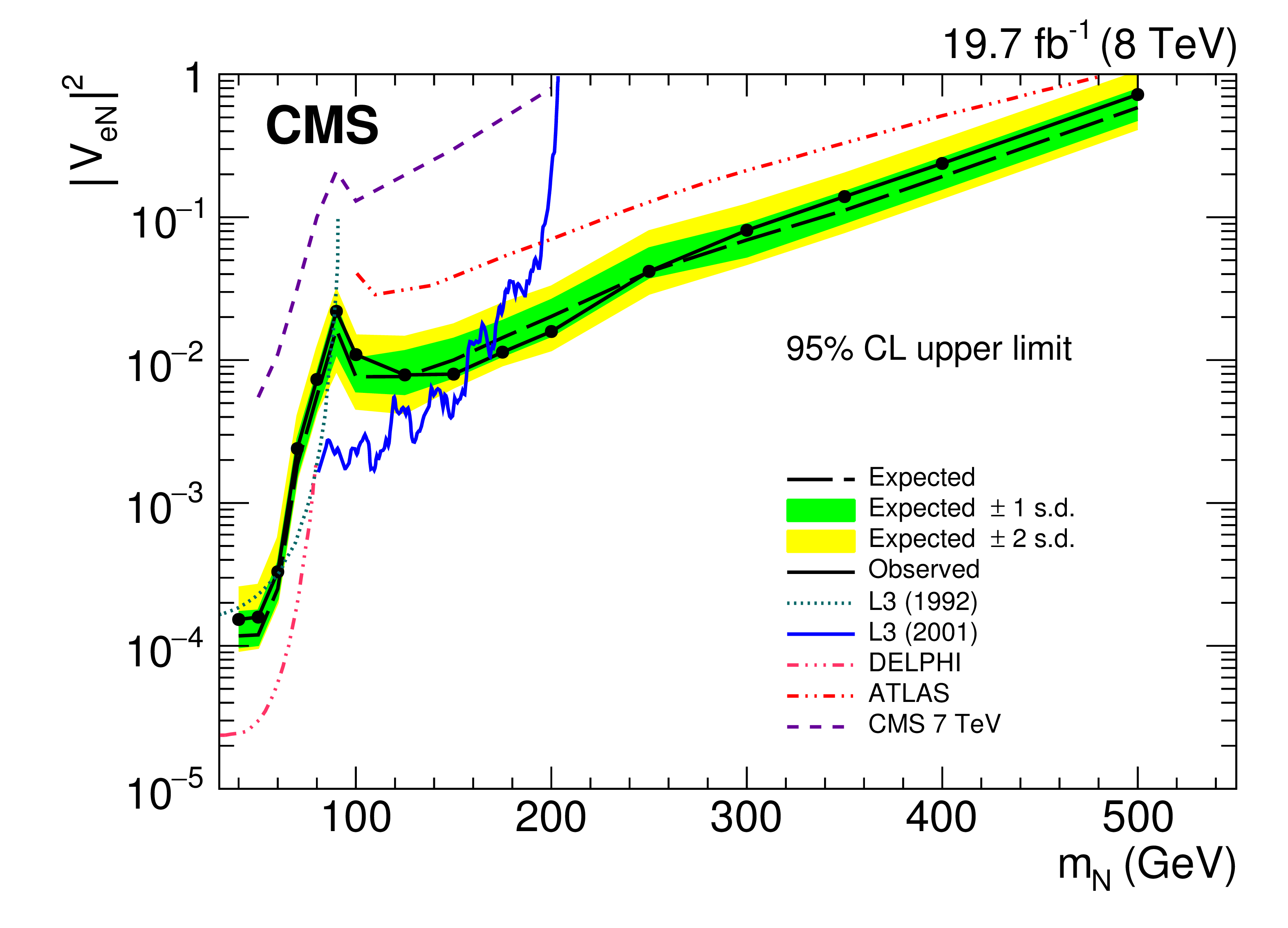
Figure 5-a:
Exclusion region at 95% CL in the $ {| {V^{}_{ {\mathrm { e }} {\mathrm {N}} }} | }^2$ vs. $ {m_{ {\mathrm {N}} }} $ plane (a) and $ {| {V^{}_{ {\mathrm { e }} {\mathrm {N}} }} | }^2$ and $ {| {V^{}_{ {\mathrm { e }} {\mathrm {N}} }} {V^{*}_{\mu {\mathrm {N}} }} | }^2 / ( | {V^{}_{ {\mathrm { e }} {\mathrm {N}} }} |^2 + | {V^{}_{\mu {\mathrm {N}} }} |^2 )$ vs. $ {m_{ {\mathrm {N}} }} $ plane (b). The dashed black curve is the expected upper limit, with one and two standard-deviation bands shown in dark green and light yellow, respectively. The solid black curve is the observed upper limit. Also shown are the upper limits from other direct searches: L3 [22,23], DELPHI [21], ATLAS [33], and the upper limits from the CMS $\sqrt {s} = 7$ TeV (2011) data [32]. |
png pdf |
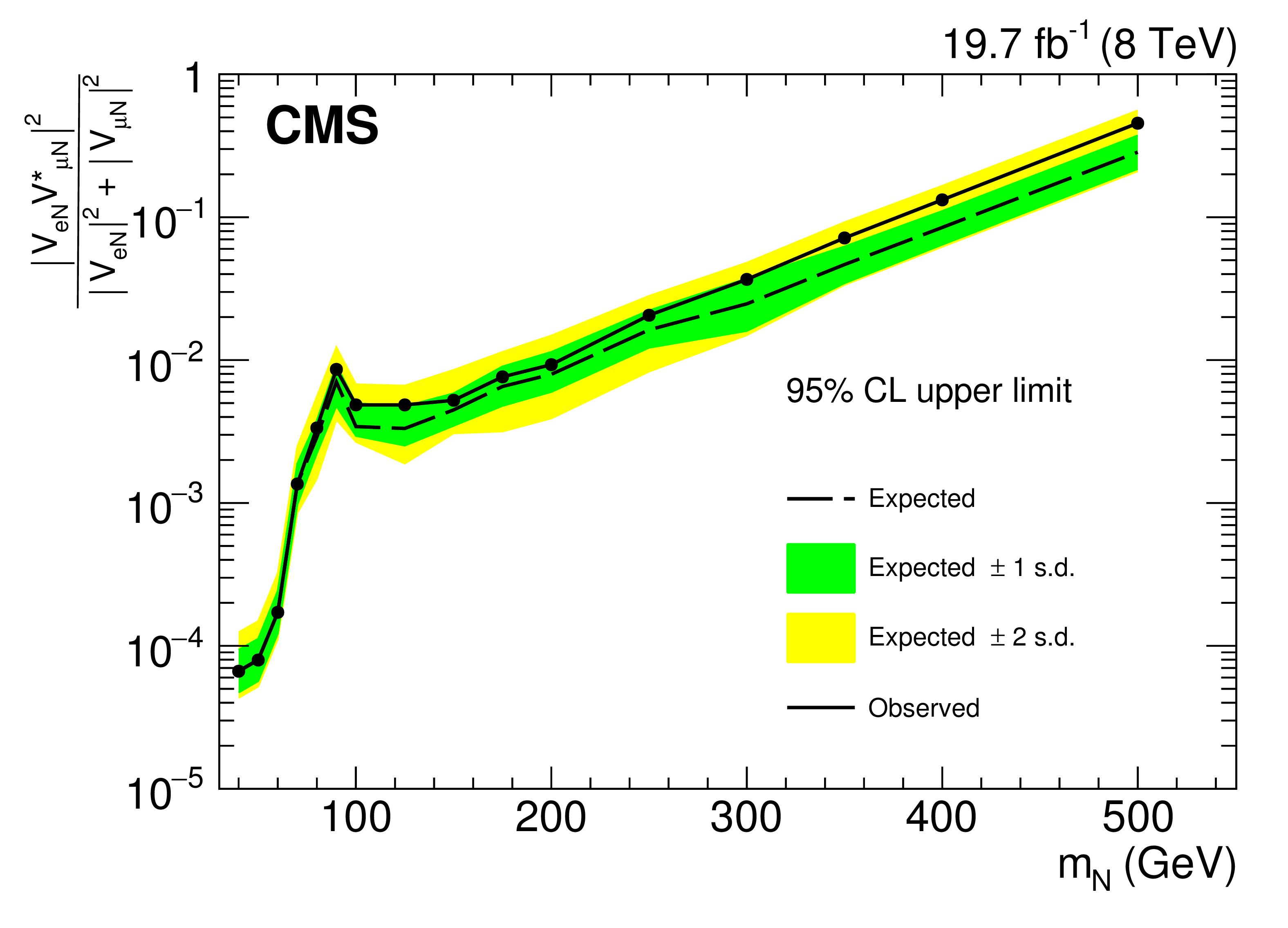
Figure 5-b:
Exclusion region at 95% CL in the $ {| {V^{}_{ {\mathrm { e }} {\mathrm {N}} }} | }^2$ vs. $ {m_{ {\mathrm {N}} }} $ plane (a) and $ {| {V^{}_{ {\mathrm { e }} {\mathrm {N}} }} | }^2$ and $ {| {V^{}_{ {\mathrm { e }} {\mathrm {N}} }} {V^{*}_{\mu {\mathrm {N}} }} | }^2 / ( | {V^{}_{ {\mathrm { e }} {\mathrm {N}} }} |^2 + | {V^{}_{\mu {\mathrm {N}} }} |^2 )$ vs. $ {m_{ {\mathrm {N}} }} $ plane (b). The dashed black curve is the expected upper limit, with one and two standard-deviation bands shown in dark green and light yellow, respectively. The solid black curve is the observed upper limit. Also shown are the upper limits from other direct searches: L3 [22,23], DELPHI [21], ATLAS [33], and the upper limits from the CMS $\sqrt {s} = 7$ TeV (2011) data [32]. |
png pdf |
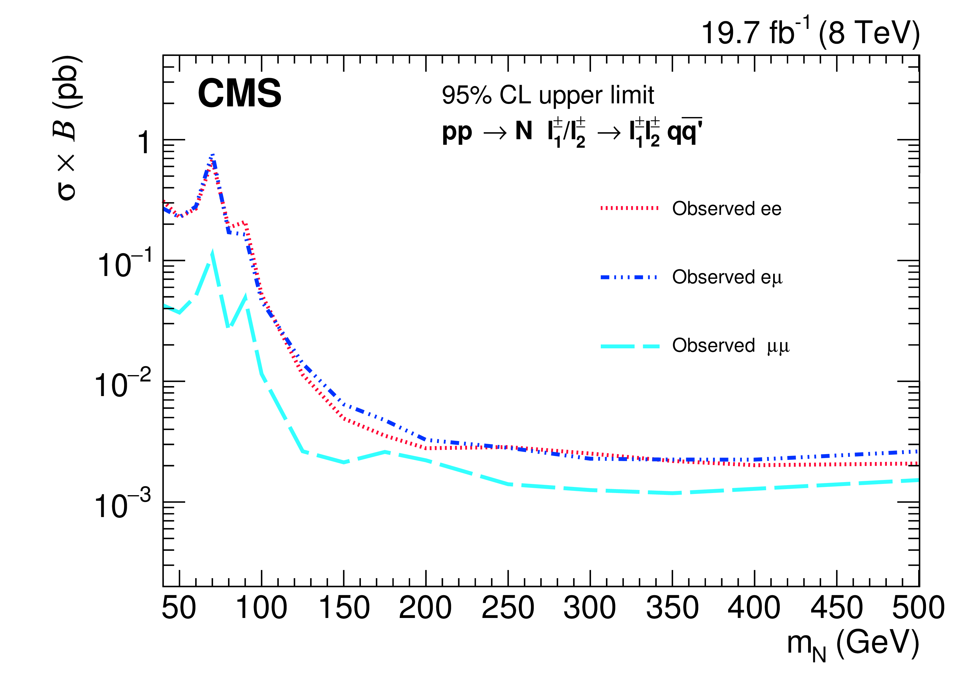
Figure 6:
Comparison of observed exclusion regions at 95% CL in the cross section times branching fraction as a function of $ {m_{ {\mathrm {N}} }} $ for $ {\mathrm { pp }} \rightarrow {\mathrm {N}} {\mathrm { e }} ^{\pm }\rightarrow {\mathrm { e }} ^{\pm } {\mathrm { e }} ^{\pm } {\mathrm { q }} {\mathrm { \bar{q} }} ^\prime $, $ {\mathrm { pp }} \rightarrow {\mathrm {N}} \mu ^{\pm } \rightarrow \mu ^{\pm } \mu ^{\pm } {\mathrm { q }} {\mathrm { \bar{q} }} ^\prime $, and $ {\mathrm { pp }} \rightarrow {\mathrm {N}} \, {\mathrm { e }} ^{\pm } / \mu ^{\pm } \rightarrow {\mathrm { e }} ^{\pm } \mu ^{\pm } {\mathrm { q }} {\mathrm { \bar{q} }} ^\prime $. The result for the dimuon channel is from Ref.[30]. |
png pdf |
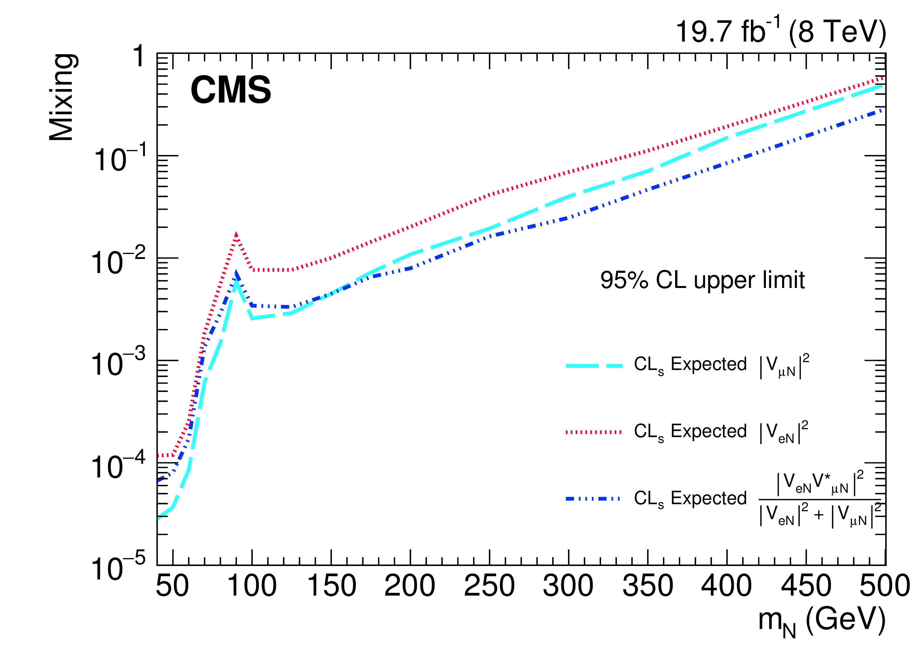
Figure 7:
Comparison of observed exclusion regions at 95% CL in $ {| {V^{}_{\mu {\mathrm {N}} }} | }^2$, $ {| {V^{}_{ {\mathrm { e }} {\mathrm {N}} }} | }^2$, and $ {| {V^{}_{ {\mathrm { e }} {\mathrm {N}} }} {V^{*}_{\mu {\mathrm {N}} }} | }^2 / ( | {V^{}_{ {\mathrm { e }} {\mathrm {N}} }} |^2 + | {V^{}_{\mu {\mathrm {N}} }} |^2 )$. The CMS result for $ {| {V^{}_{\mu {\mathrm {N}} }} | }^2$ is from Ref.[30]. |
| Tables | |
png pdf |
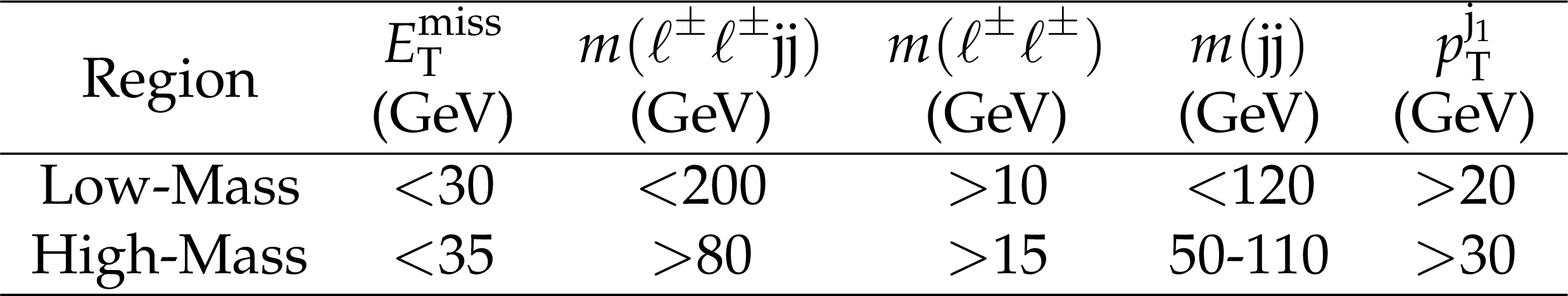
Table 1:
Selection requirements for the low- and high-mass signal regions. |
png pdf |
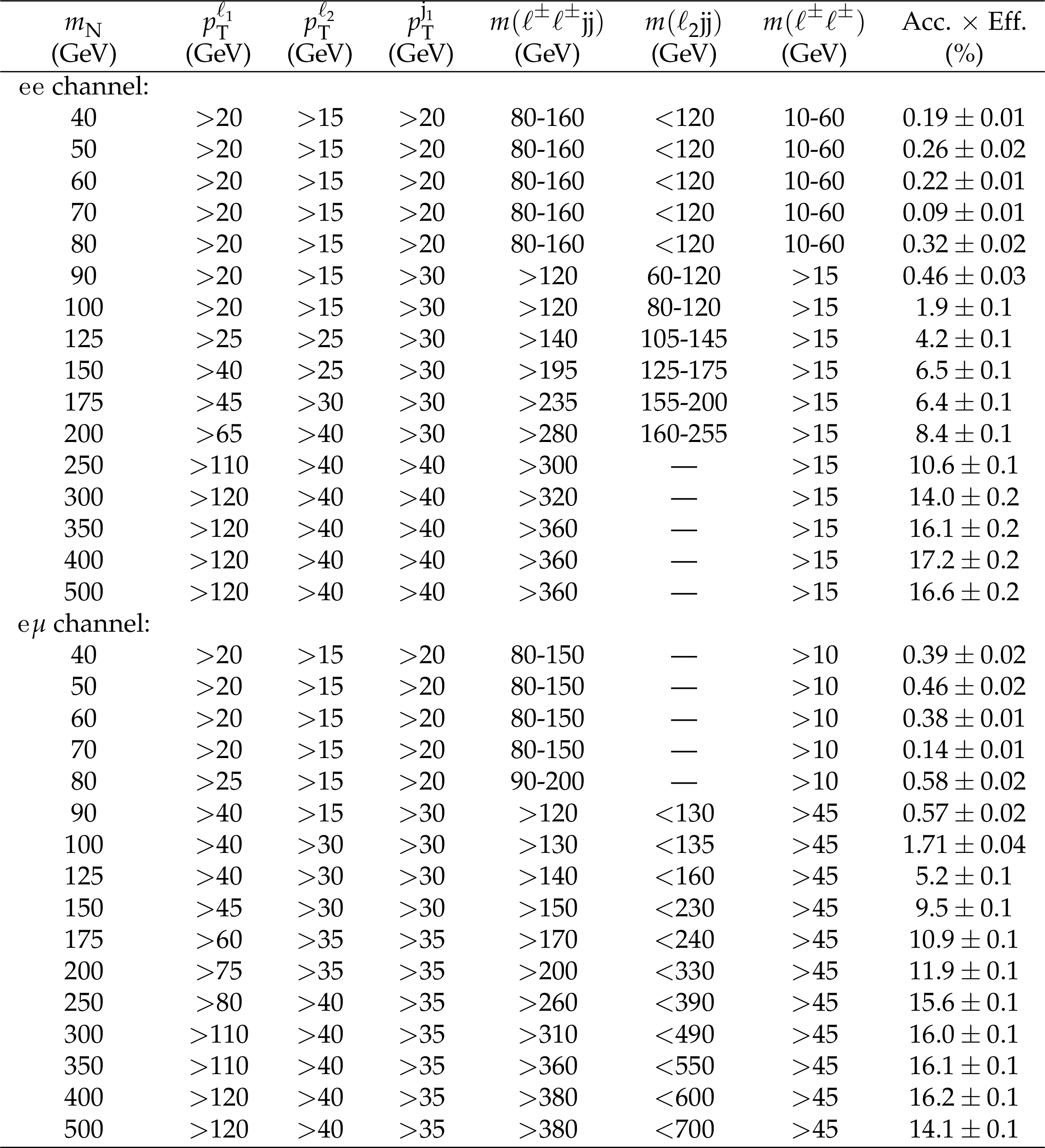
Table 2:
Selection requirements on discriminating variables determined by the optimization for each Majorana neutrino mass point. The last column shows the overall signal acceptance. Different selection criteria are used for low- and high-mass search regions. The ``---'' indicates that no selection requirement is made. |
png pdf |
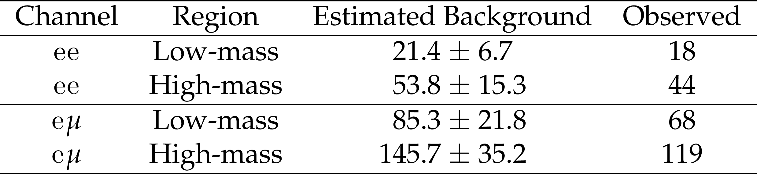
Table 3:
Observed event yields and estimated backgrounds in the low- and high-mass control regions. The uncertainty in the background yield is the sum in quadrature of the statistical and systematic uncertainties. |
png pdf |
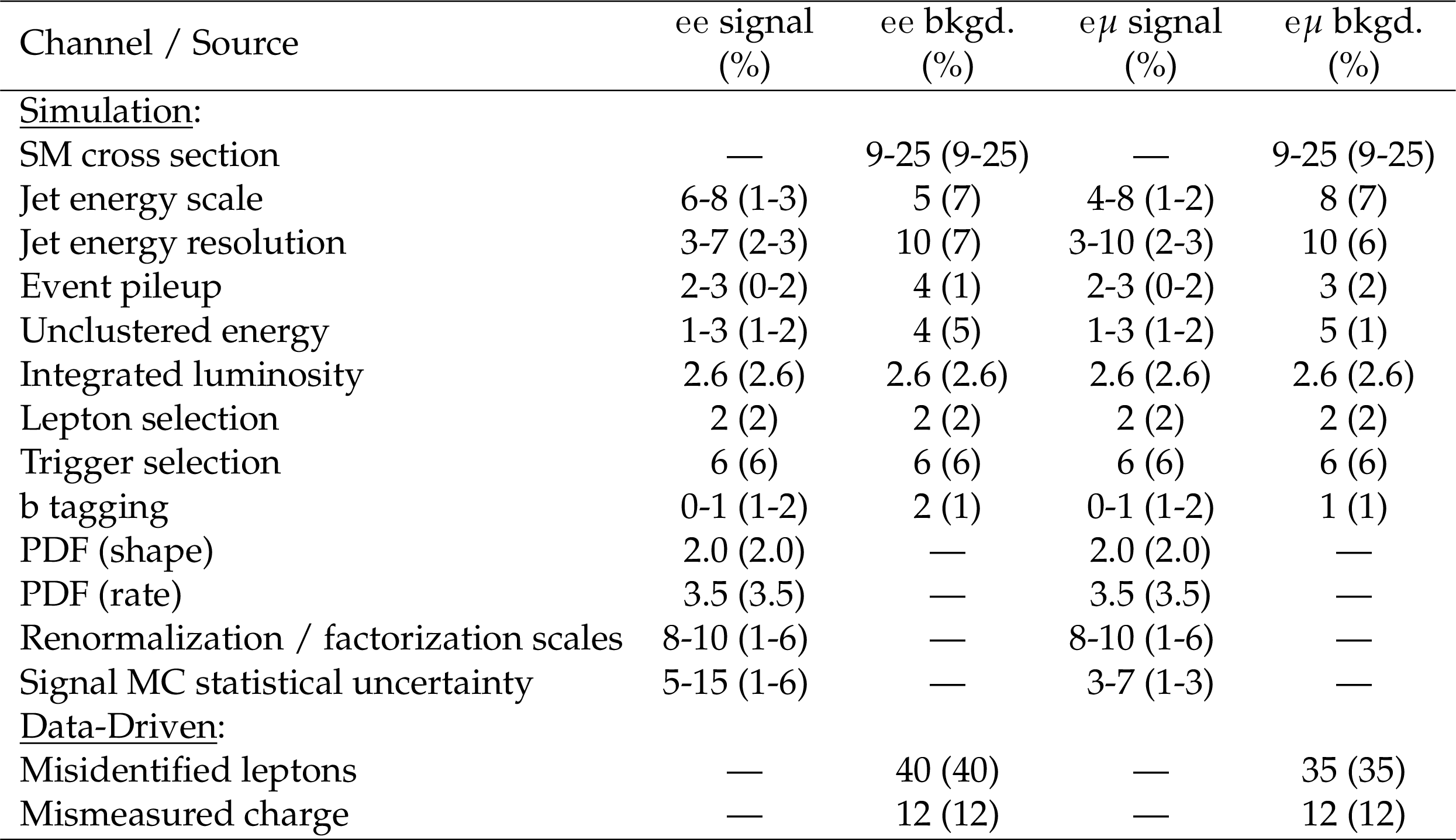
Table 4:
Summary of the relative systematic uncertainties in heavy Majorana neutrino signal yields and the background from prompt same-sign leptons, both estimated from simulation. The relative systematic uncertainties assigned to the data-driven backgrounds for the misidentified lepton background and mismeasured charge background are also shown. The uncertainties are given for the low-mass (high-mass) selections. |
png pdf |
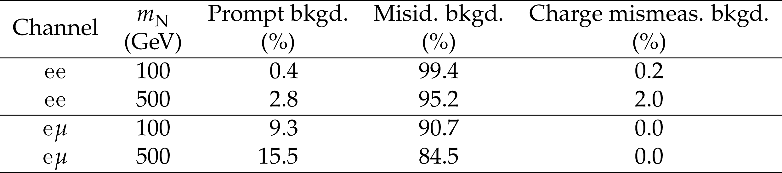
Table 5:
Summary of contributions to the systematic uncertainty related to the prompt same-sign leptons background, misidentified lepton background, and mismeasured charge background on the total background uncertainty for the case of $ {m_{ {\mathrm {N}} }} =$ 100 and 500 GeV. |
png pdf |
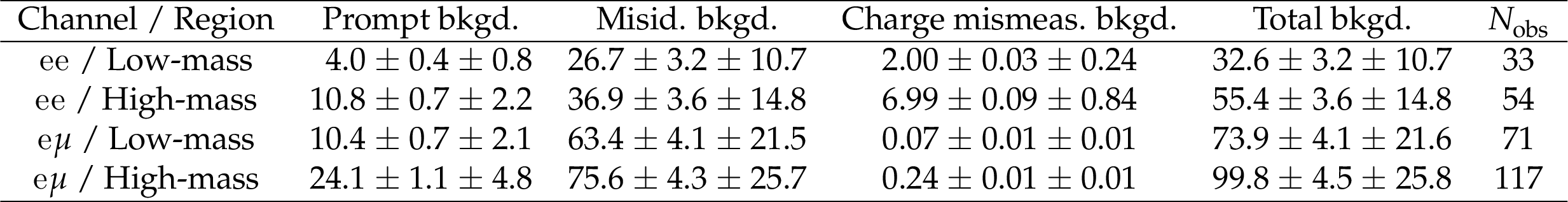
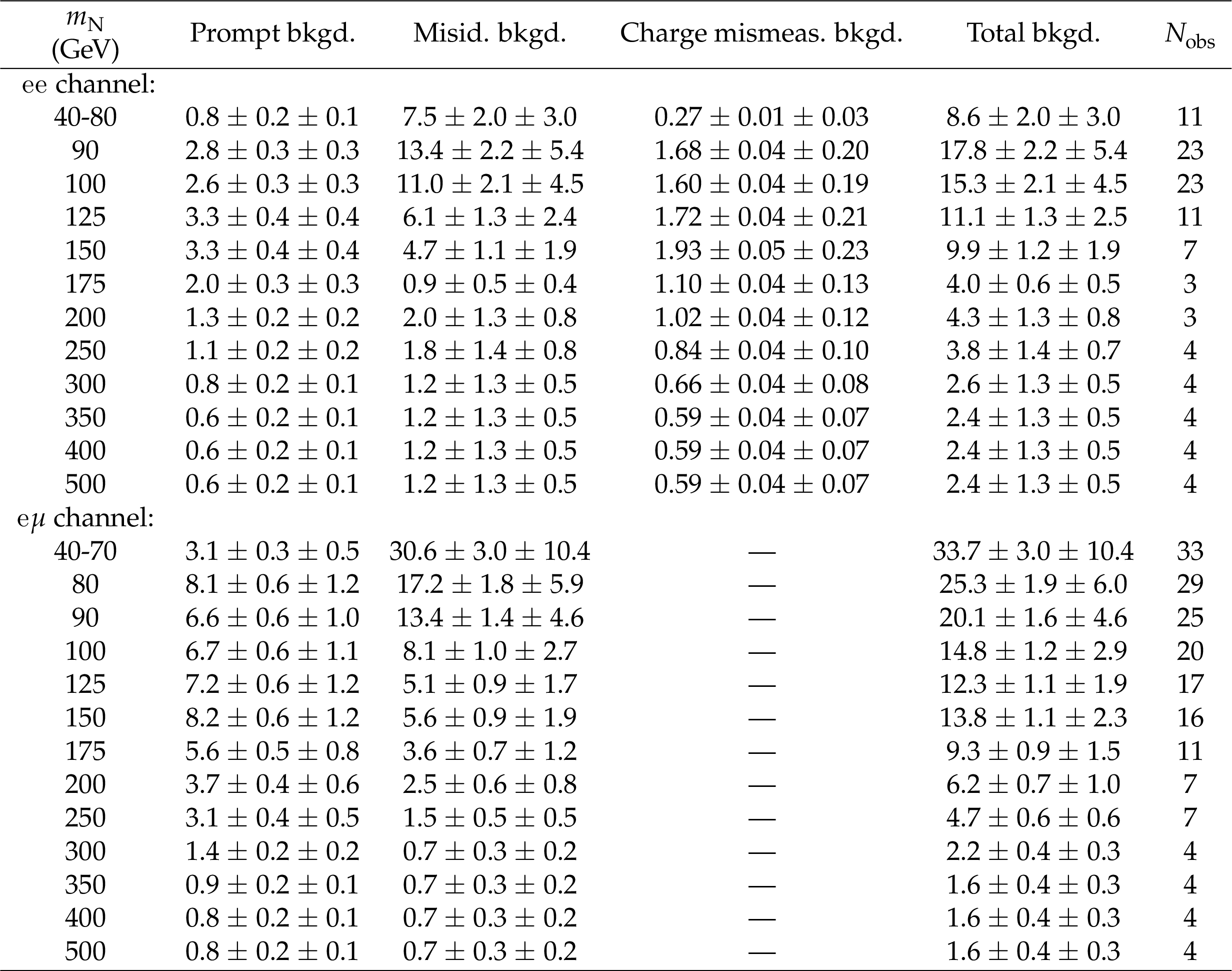
Table 6:
Observed event yields and estimated backgrounds after the application of all selection, except for the final optimization. The background predictions from prompt same-sign leptons (Prompt bkgd.), misidentified leptons (Misid. bkgd.), mismeasured charge (Charge mismeas. bkgd.) and the total background (Total bkgd.) are shown together with the number of events observed in data. The uncertainties shown are the statistical and systematic components, respectively. |
png pdf |
Table 7:
Dielectron and electron-muon channel results after final optimization. The background predictions from prompt same-sign leptons, misidentified leptons, and mismeasured charge are shown along with the total background estimate and the number of events observed in data. The uncertainties shown are the statistical and systematic components, respectively. |
| Summary |
| A search for heavy Majorana neutrinos in $ \mathrm{ e^{\pm} e^{\pm} j j } $ and $ \mathrm{ e^{\pm} \mu^{\pm} j j } $events has been performed using 19.7 fb$^{-1}$ of data collected during 2012 in pp collisions at a centre-of-mass energy of 8 TeV. No excess of events compared to the expected standard model background prediction is observed.Upper limits at 95% CL are set on $| \mathrm{V_{eN}} |^2$ and $| \mathrm{V_{eN}} \mathrm{V^{*}_{\mu N}} |^2 / ( | \mathrm{V_{eN}} |^2 + | \mathrm{V_{\mu N}} |^2 )$ as a function of $ m_{\mathrm{ N }} $ in the range $ m_{\mathrm{ N }} =$ 40-500 GeV, where $ \mathrm{V_{\ell N}} $ is the mixing element of the heavy neutrino N with the standard model neutrino $\nu_{\ell}$.A significant increase in sensitivity on the limits for $| \mathrm{V_{eN}} |^2$ has been achieved over the previous limits set by CMS with the 7 TeV data. These limits are the most restrictive direct limits for heavy Majorana neutrino masses above 200 GeV. The limits on $| \mathrm{V_{eN}} |^2$ and $| \mathrm{V_{eN}} \mathrm{V^{*}_{\mu N}} |^2 / ( | \mathrm{V_{eN}} |^2 + | \mathrm{V_{\mu N}} |^2 )$ presented here are the first direct limits on this quantity for $ m_{\mathrm{ N }} $ above 40 GeV. For $ m_{\mathrm{ N }} $ = 90 GeV the limits are $| \mathrm{V_{eN}} |^2 <$ 0.020 and $| \mathrm{V_{eN}} \mathrm{V^{*}_{\mu N}} |^2 / ( | \mathrm{V_{eN}} |^2 + | \mathrm{V_{\mu N}} |^2 ) <$ 0.005. At $ m_{\mathrm{ N }} $ = 200 GeV the limits are $| \mathrm{V_{eN}} |^2 <$ 0.017 and $| \mathrm{V_{eN}} \mathrm{V^{*}_{\mu N}} |^2 / ( | \mathrm{V_{eN}} |^2 + | \mathrm{V_{\mu N}} |^2 ) <$ 0.005, and at $ m_{\mathrm{ N }} $ = 500 GeV they are $| \mathrm{V_{eN}} |^2 <$ 0.71 and $| \mathrm{V_{eN}} \mathrm{V^{*}_{\mu N}} |^2 / ( | \mathrm{V_{eN}} |^2 + | \mathrm{V_{\mu N}} |^2 ) <$ 0.29. |
|
|
Compact Muon Solenoid LHC, CERN |
|

|

|

|

|

|