

Compact Muon Solenoid
LHC, CERN
| CMS-FSQ-12-035 ; CERN-PH-EP-2014-234 | ||
| Measurement of electroweak production of two jets in association with a Z boson in proton-proton collisions at $ \sqrt{s} = $ 8 TeV | ||
| CMS Collaboration | ||
| 13 October 2014 | ||
| Eur. Phys. J. C 75 (2015) 66 | ||
| Abstract: The purely electroweak (EW) cross section for the production of two jets in association with a Z boson, in proton-proton collisions at $ \sqrt{s} = $ 8 TeV, is measured using data recorded by the CMS experiment at the CERN LHC, corresponding to an integrated luminosity of 19.7 fb$^{-1}$. The electroweak cross section for the $\ell\ell j j $ final state (with $\ell = \mathrm{ e }$ or $\mu$ and j representing the quarks produced in the hard interaction) in the kinematic region defined by $M_{\ell\ell} > $ 50 GeV, $M_\mathrm{jj} > $ 120 GeV, transverse momentum $p_{\mathrm{T}}^j > $ 25 GeV, and pseudorapidity $| {\eta_\mathrm{j}} | < $ 5 , is found to be $\sigma_\mathrm{EW}(\ell\ell j j )=$ 174 $\pm$ 15 (stat) $\pm$ 40 (syst) fb, in agreement with the standard model prediction. The associated jet activity of the selected events is studied, in particular in a signal-enriched region of phase space, and the measurements are found to be in agreement with QCD predictions. | ||
| Links: e-print arXiv:1410.3153 [hep-ex] (PDF) ; CDS record ; inSPIRE record ; Public twiki page ; CADI line (restricted) ; | ||
| Figures | |

png pdf |
Figure 1-a:
Representative Feynman diagrams for dilepton production in association with two jets from purely electroweak contributions: (left) vector boson fusion, (middle) bremsstrahlung-like, and (right) multiperipheral production. |

png pdf |
Figure 1-b:
Representative Feynman diagrams for dilepton production in association with two jets from purely electroweak contributions: (left) vector boson fusion, (middle) bremsstrahlung-like, and (right) multiperipheral production. |

png pdf |
Figure 1-c:
Representative Feynman diagrams for dilepton production in association with two jets from purely electroweak contributions: (left) vector boson fusion, (middle) bremsstrahlung-like, and (right) multiperipheral production. |

png pdf |
Figure 2-a:
Representative diagrams for order $\alpha _\mathrm {S}^2$ corrections to DY production that comprise the main background (B) in this study. |

png pdf |
Figure 2-b:
Representative diagrams for order $\alpha _\mathrm {S}^2$ corrections to DY production that comprise the main background (B) in this study. |
png pdf |
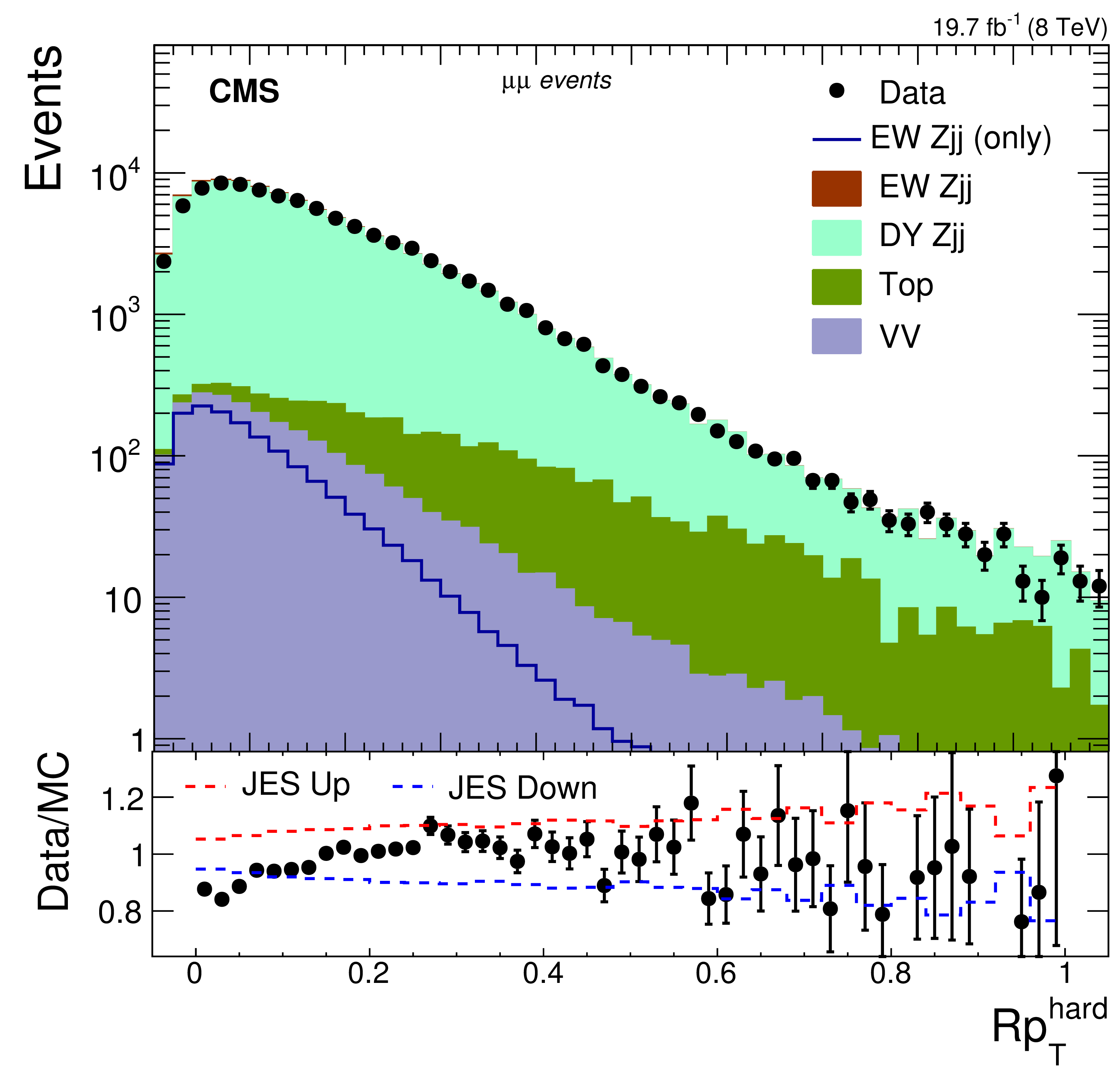
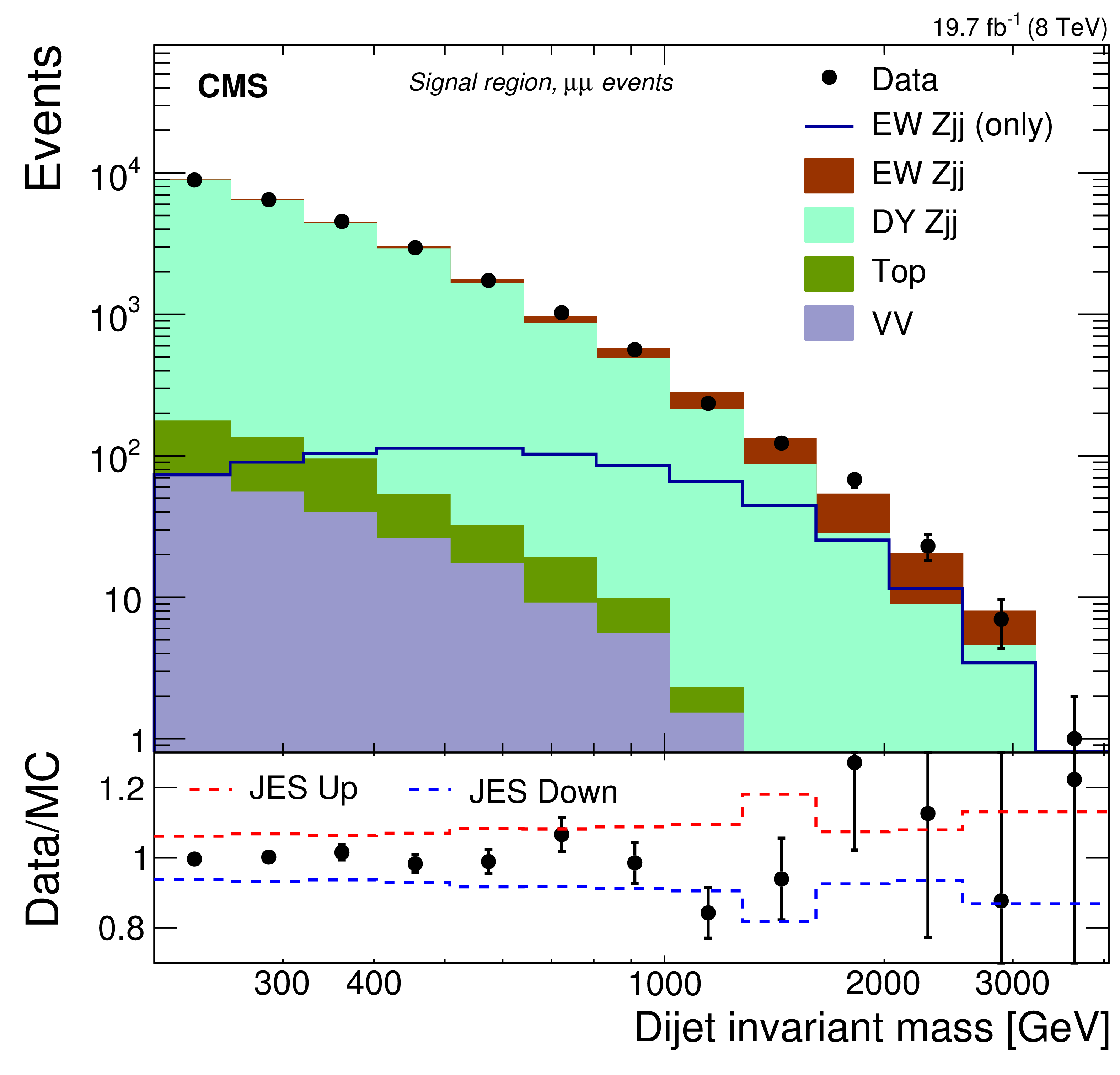
Figure 3-a:
Distribution for (left) $R {p_{\mathrm {T}}} ^\text {hard}$ and $M_\mathrm {jj}$ for $\mu \mu $ events with (middle) $R {p_{\mathrm {T}}} ^\text {hard}\geq 0.14$ (control region) and (right) $R {p_{\mathrm {T}}} ^\text {hard}< $ 0.14 (signal region). The contributions from the different background sources and the signal are shown stacked, with data points superimposed. The panels below the distributions show the ratio between the data and expectations as well as the uncertainty envelope for the impact of the uncertainty of the JES. |

png pdf |
Figure 3-b:
Distribution for (left) $R {p_{\mathrm {T}}} ^\text {hard}$ and $M_\mathrm {jj}$ for $\mu \mu $ events with (middle) $R {p_{\mathrm {T}}} ^\text {hard}\geq 0.14$ (control region) and (right) $R {p_{\mathrm {T}}} ^\text {hard}< $ 0.14 (signal region). The contributions from the different background sources and the signal are shown stacked, with data points superimposed. The panels below the distributions show the ratio between the data and expectations as well as the uncertainty envelope for the impact of the uncertainty of the JES. |
png pdf |
Figure 3-c:
Distribution for (left) $R {p_{\mathrm {T}}} ^\text {hard}$ and $M_\mathrm {jj}$ for $\mu \mu $ events with (middle) $R {p_{\mathrm {T}}} ^\text {hard}\geq 0.14$ (control region) and (right) $R {p_{\mathrm {T}}} ^\text {hard}< $ 0.14 (signal region). The contributions from the different background sources and the signal are shown stacked, with data points superimposed. The panels below the distributions show the ratio between the data and expectations as well as the uncertainty envelope for the impact of the uncertainty of the JES. |
png pdf |
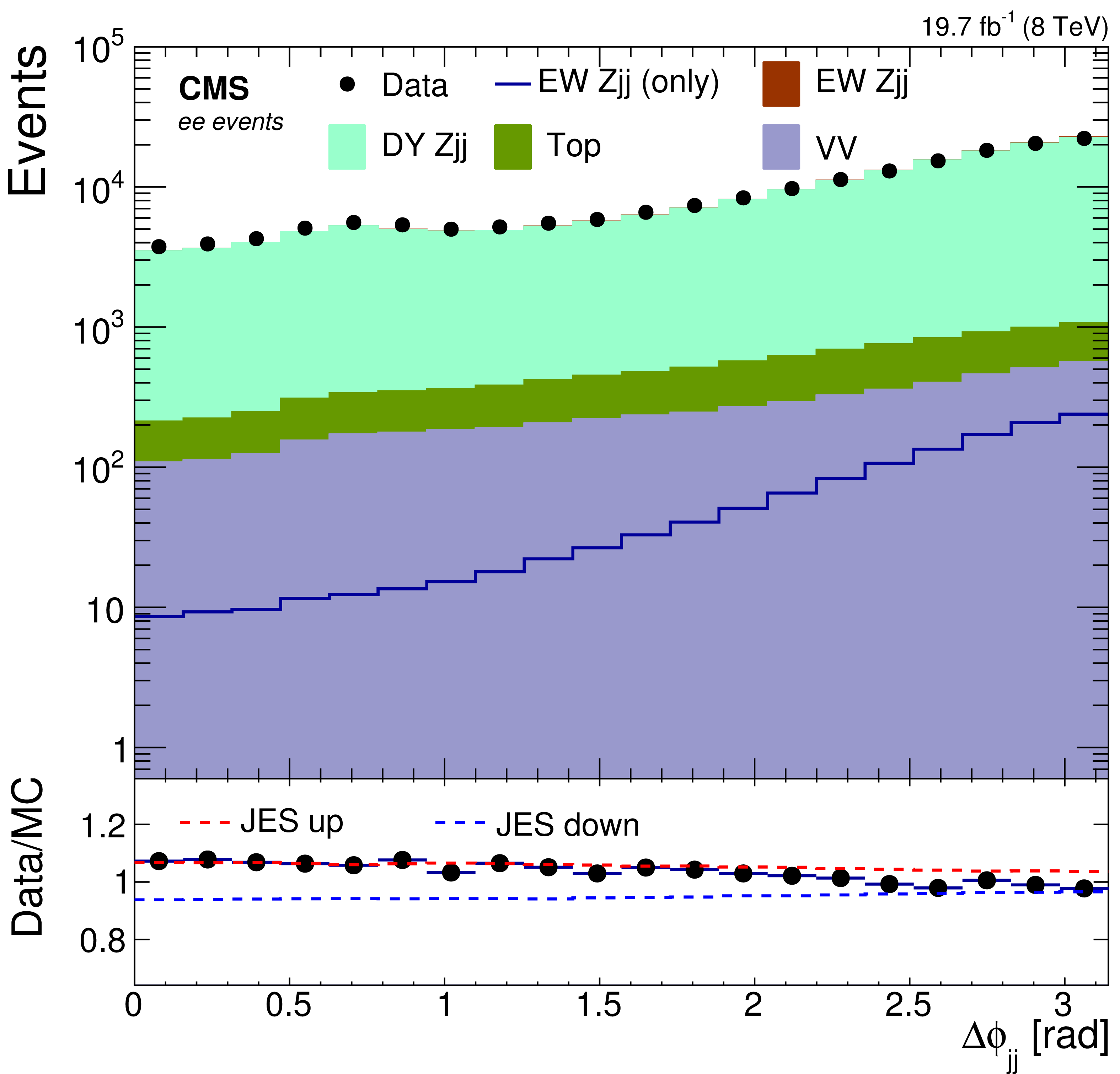
Figure 4-a:
Distribution for (left) the difference in the azimuthal angle and (middle) difference in the pseudorapidity of the tagging jets for ee events, with $R {p_{\mathrm {T}}} ^\text {hard}\geq 0.14$. The $z^*$ distribution (right) is shown for the same category of events. The panels below the distributions show the ratio between the data and expectations as well as the uncertainty envelope for the impact of the uncertainty of the JES. |

png pdf |
Figure 4-b:
Distribution for (left) the difference in the azimuthal angle and (middle) difference in the pseudorapidity of the tagging jets for ee events, with $R {p_{\mathrm {T}}} ^\text {hard}\geq 0.14$. The $z^*$ distribution (right) is shown for the same category of events. The panels below the distributions show the ratio between the data and expectations as well as the uncertainty envelope for the impact of the uncertainty of the JES. |

png pdf |
Figure 4-c:
Distribution for (left) the difference in the azimuthal angle and (middle) difference in the pseudorapidity of the tagging jets for ee events, with $R {p_{\mathrm {T}}} ^\text {hard}\geq 0.14$. The $z^*$ distribution (right) is shown for the same category of events. The panels below the distributions show the ratio between the data and expectations as well as the uncertainty envelope for the impact of the uncertainty of the JES. |
png pdf |
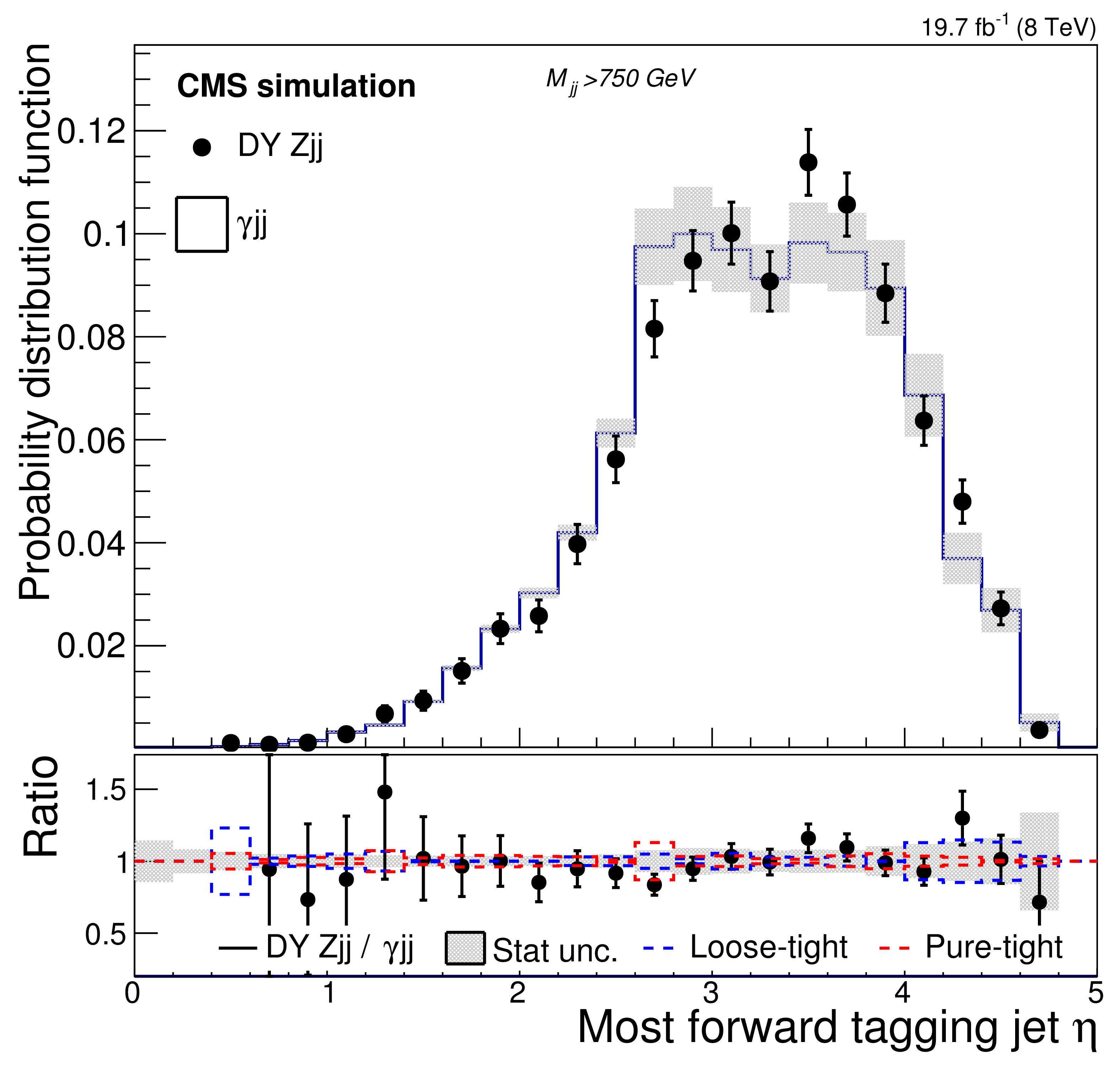
Figure 5-a:
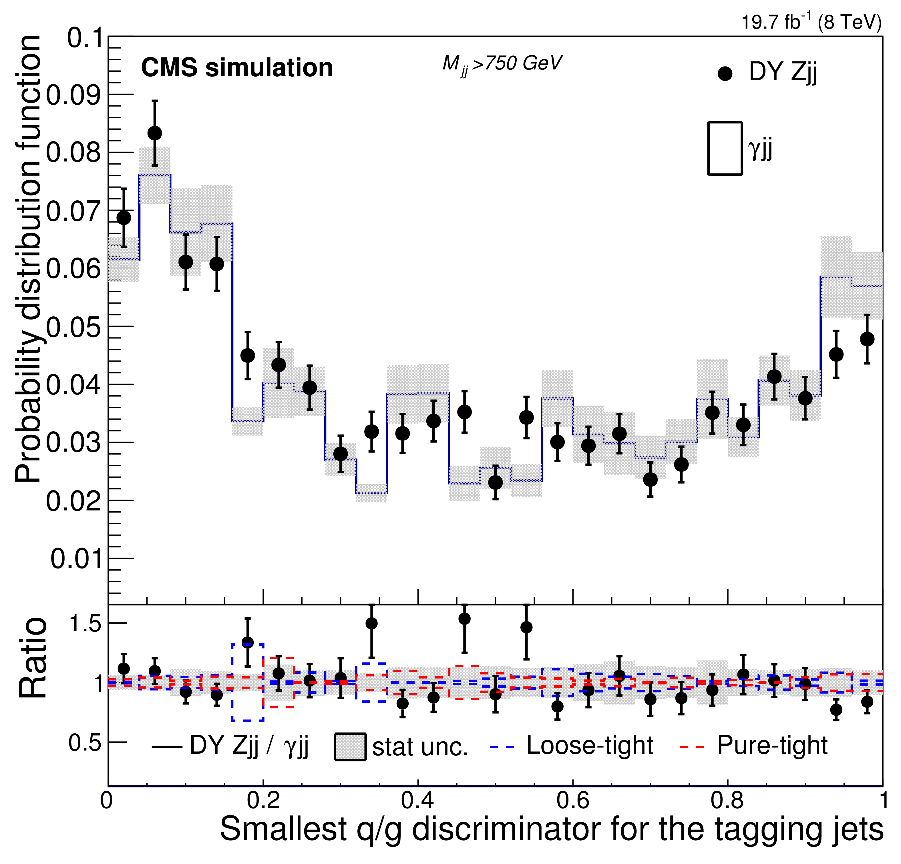
Comparison of the ${\mathrm {DY} \mathrm{ Z } \mathrm {jj}} $ distributions with the prediction from the photon control sample, for simulated events with $M_\mathrm {jj}> $ 750 GeV. The upper left subfigure shows the distributions in the pseudorapidity $\eta $ of the most forward tagging jet and the upper right shows the smallest q/g discriminant of the two tagging jets. The lower left shows the pseudorapidity separation $\Delta \eta _\mathrm {jj}$ and the lower right the relative ${p_{\mathrm {T}}}$ balance of the tagging jets $\Delta ^\text {rel}_{ {p_{\mathrm {T}}} }$. The DY ${\gamma \mathrm {jj}} $ distribution contains the contribution from prompt and misidentified photons as estimated from simulation and it is compared to the simulated ${\mathrm {DY} \mathrm{ Z } \mathrm {jj}} $ sample in the top panel of each subfigure. The bottom panels show the ratio between the ${\mathrm {DY} \mathrm{ Z } \mathrm {jj}} $ distribution and the photon-based prediction, and includes the different sources of estimated total uncertainty in the background shape from the photon control sample. (See text for specification of impact of loose, tight and pure photons). |
png pdf |
Figure 5-b:
Comparison of the ${\mathrm {DY} \mathrm{ Z } \mathrm {jj}} $ distributions with the prediction from the photon control sample, for simulated events with $M_\mathrm {jj}> $ 750 GeV. The upper left subfigure shows the distributions in the pseudorapidity $\eta $ of the most forward tagging jet and the upper right shows the smallest q/g discriminant of the two tagging jets. The lower left shows the pseudorapidity separation $\Delta \eta _\mathrm {jj}$ and the lower right the relative ${p_{\mathrm {T}}}$ balance of the tagging jets $\Delta ^\text {rel}_{ {p_{\mathrm {T}}} }$. The DY ${\gamma \mathrm {jj}} $ distribution contains the contribution from prompt and misidentified photons as estimated from simulation and it is compared to the simulated ${\mathrm {DY} \mathrm{ Z } \mathrm {jj}} $ sample in the top panel of each subfigure. The bottom panels show the ratio between the ${\mathrm {DY} \mathrm{ Z } \mathrm {jj}} $ distribution and the photon-based prediction, and includes the different sources of estimated total uncertainty in the background shape from the photon control sample. (See text for specification of impact of loose, tight and pure photons). |

png pdf |
Figure 5-c:
Comparison of the ${\mathrm {DY} \mathrm{ Z } \mathrm {jj}} $ distributions with the prediction from the photon control sample, for simulated events with $M_\mathrm {jj}> $ 750 GeV. The upper left subfigure shows the distributions in the pseudorapidity $\eta $ of the most forward tagging jet and the upper right shows the smallest q/g discriminant of the two tagging jets. The lower left shows the pseudorapidity separation $\Delta \eta _\mathrm {jj}$ and the lower right the relative ${p_{\mathrm {T}}}$ balance of the tagging jets $\Delta ^\text {rel}_{ {p_{\mathrm {T}}} }$. The DY ${\gamma \mathrm {jj}} $ distribution contains the contribution from prompt and misidentified photons as estimated from simulation and it is compared to the simulated ${\mathrm {DY} \mathrm{ Z } \mathrm {jj}} $ sample in the top panel of each subfigure. The bottom panels show the ratio between the ${\mathrm {DY} \mathrm{ Z } \mathrm {jj}} $ distribution and the photon-based prediction, and includes the different sources of estimated total uncertainty in the background shape from the photon control sample. (See text for specification of impact of loose, tight and pure photons). |

png pdf |
Figure 5-d:
Comparison of the ${\mathrm {DY} \mathrm{ Z } \mathrm {jj}} $ distributions with the prediction from the photon control sample, for simulated events with $M_\mathrm {jj}> $ 750 GeV. The upper left subfigure shows the distributions in the pseudorapidity $\eta $ of the most forward tagging jet and the upper right shows the smallest q/g discriminant of the two tagging jets. The lower left shows the pseudorapidity separation $\Delta \eta _\mathrm {jj}$ and the lower right the relative ${p_{\mathrm {T}}}$ balance of the tagging jets $\Delta ^\text {rel}_{ {p_{\mathrm {T}}} }$. The DY ${\gamma \mathrm {jj}} $ distribution contains the contribution from prompt and misidentified photons as estimated from simulation and it is compared to the simulated ${\mathrm {DY} \mathrm{ Z } \mathrm {jj}} $ sample in the top panel of each subfigure. The bottom panels show the ratio between the ${\mathrm {DY} \mathrm{ Z } \mathrm {jj}} $ distribution and the photon-based prediction, and includes the different sources of estimated total uncertainty in the background shape from the photon control sample. (See text for specification of impact of loose, tight and pure photons). |
png pdf |
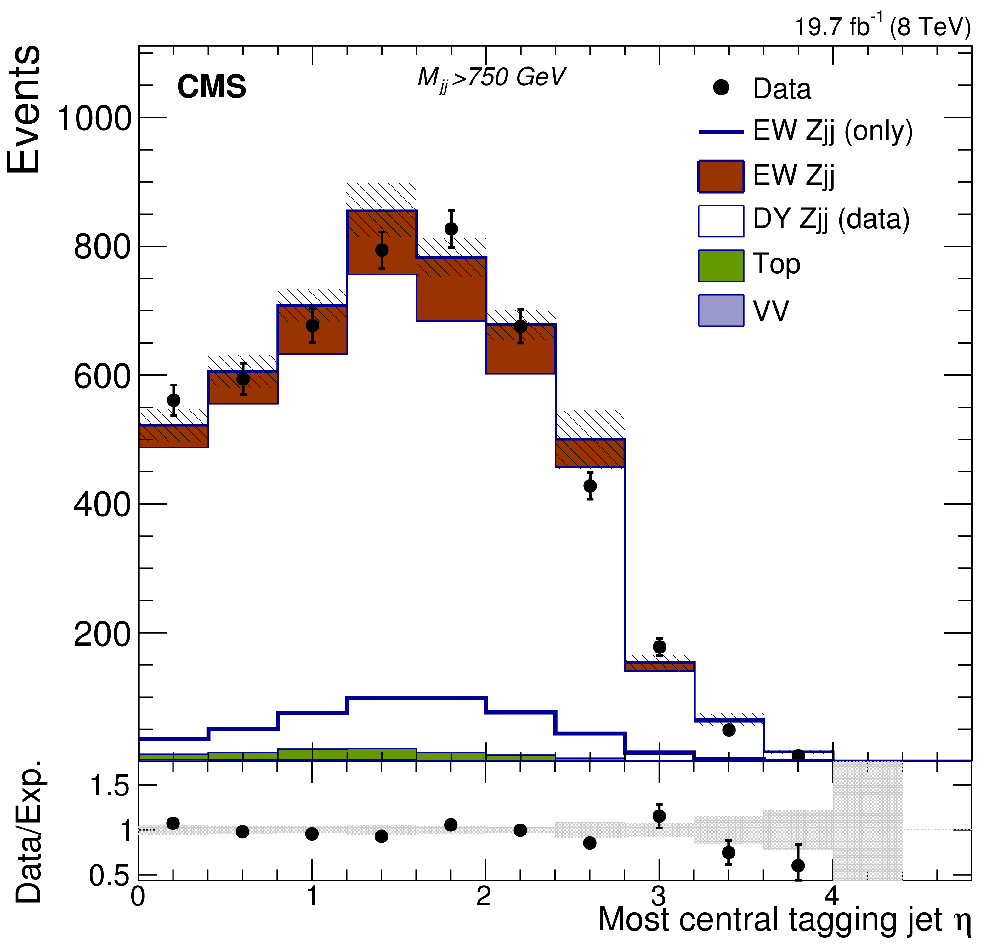
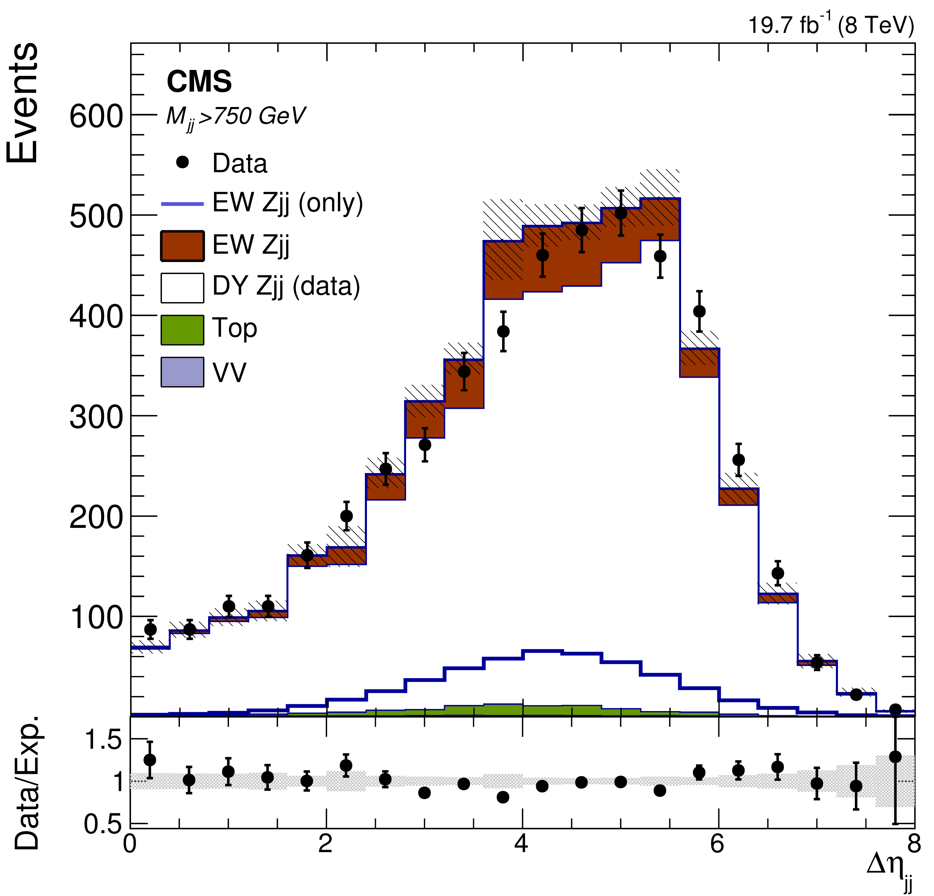
Figure 6-a:
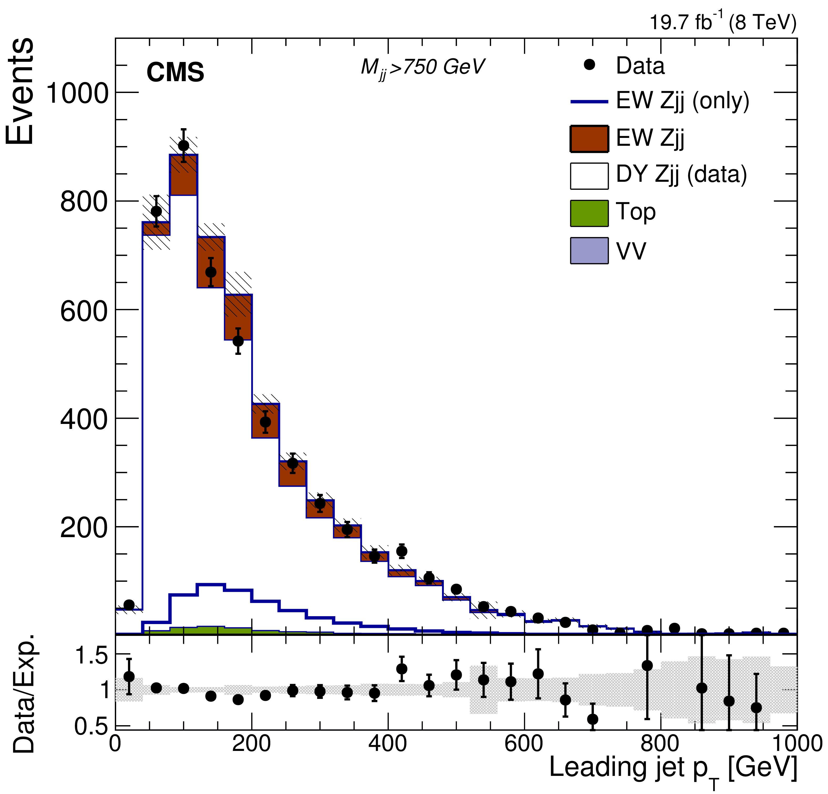
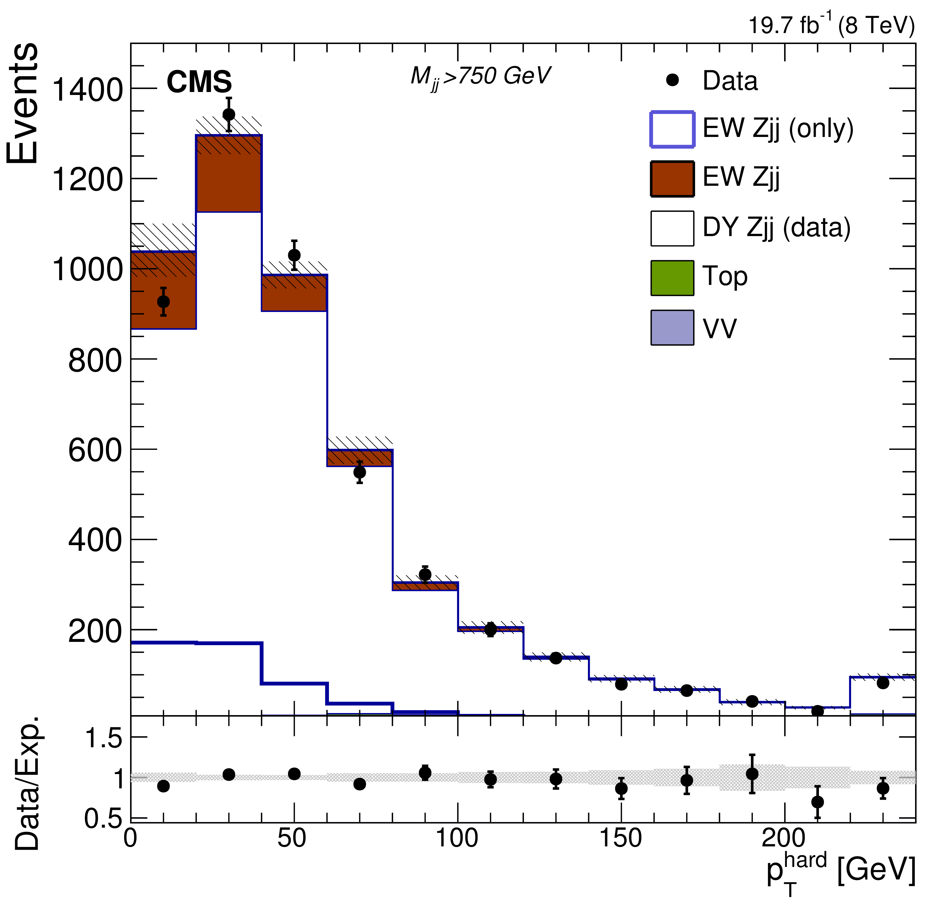
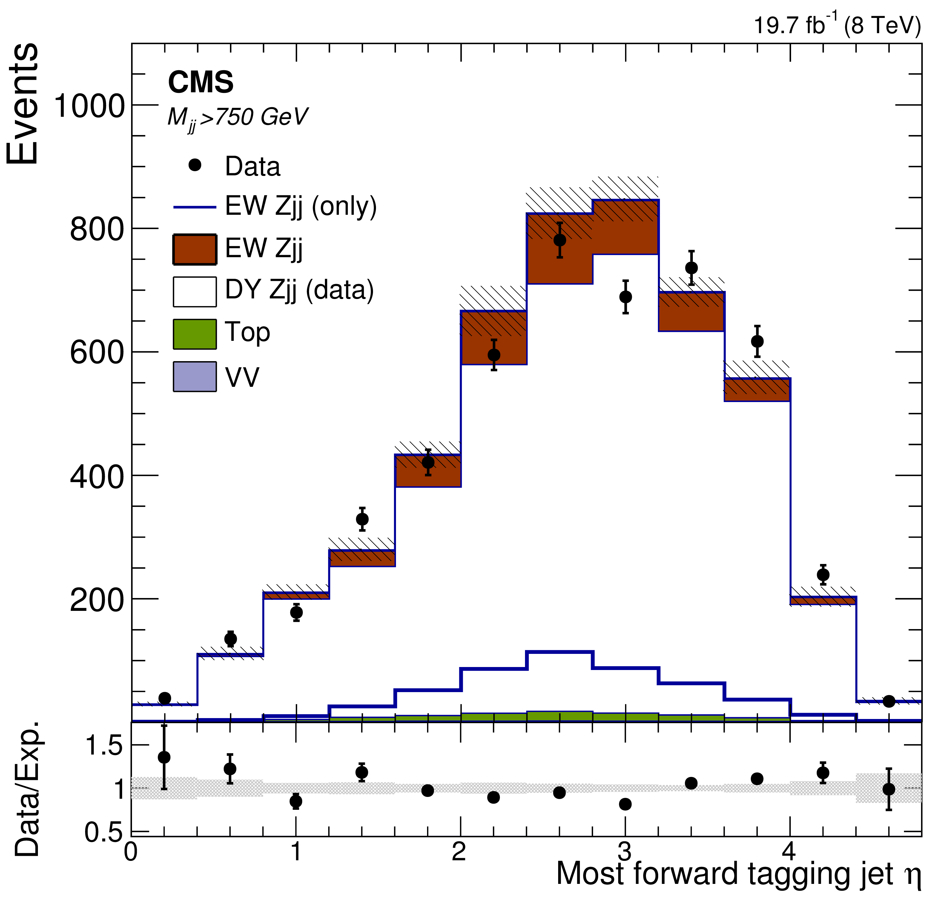
Distributions for the tagging jets for $M_\mathrm {jj}> $ 750 GeV in the combined dielectron and dimuon event sample: (upper left) ${p_{\mathrm {T}}}$ of the leading jet, (upper right) ${p_{\mathrm {T}}}$ of the sub-leading jet, (middle left) hard process ${p_{\mathrm {T}}} (dijet+\mathrm{ Z } $ system), (middle right) $\eta $ of the most forward jet, (lower left) $\eta $ of the most central jet and (lower right) $\Delta \eta _\mathrm {jj}$ of the tagging jets. In the top panels, the contributions from the different background sources and the signal are shown stacked being data superimposed. In all plots the signal shape is also superimposed separately as a thick line. The bottom panels show the ratio between data and total prediction. The total uncertainty assigned to the ${\mathrm {DY} \mathrm{ Z } \mathrm {jj}} $ background estimate from ${\gamma \mathrm {jj}} $ control sample in data is shown in all panels as a shaded grey band. |

png pdf |
Figure 6-b:
Distributions for the tagging jets for $M_\mathrm {jj}> $ 750 GeV in the combined dielectron and dimuon event sample: (upper left) ${p_{\mathrm {T}}}$ of the leading jet, (upper right) ${p_{\mathrm {T}}}$ of the sub-leading jet, (middle left) hard process ${p_{\mathrm {T}}} (dijet+\mathrm{ Z } $ system), (middle right) $\eta $ of the most forward jet, (lower left) $\eta $ of the most central jet and (lower right) $\Delta \eta _\mathrm {jj}$ of the tagging jets. In the top panels, the contributions from the different background sources and the signal are shown stacked being data superimposed. In all plots the signal shape is also superimposed separately as a thick line. The bottom panels show the ratio between data and total prediction. The total uncertainty assigned to the ${\mathrm {DY} \mathrm{ Z } \mathrm {jj}} $ background estimate from ${\gamma \mathrm {jj}} $ control sample in data is shown in all panels as a shaded grey band. |
png pdf |
Figure 6-c:
Distributions for the tagging jets for $M_\mathrm {jj}> $ 750 GeV in the combined dielectron and dimuon event sample: (upper left) ${p_{\mathrm {T}}}$ of the leading jet, (upper right) ${p_{\mathrm {T}}}$ of the sub-leading jet, (middle left) hard process ${p_{\mathrm {T}}} (dijet+\mathrm{ Z } $ system), (middle right) $\eta $ of the most forward jet, (lower left) $\eta $ of the most central jet and (lower right) $\Delta \eta _\mathrm {jj}$ of the tagging jets. In the top panels, the contributions from the different background sources and the signal are shown stacked being data superimposed. In all plots the signal shape is also superimposed separately as a thick line. The bottom panels show the ratio between data and total prediction. The total uncertainty assigned to the ${\mathrm {DY} \mathrm{ Z } \mathrm {jj}} $ background estimate from ${\gamma \mathrm {jj}} $ control sample in data is shown in all panels as a shaded grey band. |
png pdf |
Figure 6-d:
Distributions for the tagging jets for $M_\mathrm {jj}> $ 750 GeV in the combined dielectron and dimuon event sample: (upper left) ${p_{\mathrm {T}}}$ of the leading jet, (upper right) ${p_{\mathrm {T}}}$ of the sub-leading jet, (middle left) hard process ${p_{\mathrm {T}}} (dijet+\mathrm{ Z } $ system), (middle right) $\eta $ of the most forward jet, (lower left) $\eta $ of the most central jet and (lower right) $\Delta \eta _\mathrm {jj}$ of the tagging jets. In the top panels, the contributions from the different background sources and the signal are shown stacked being data superimposed. In all plots the signal shape is also superimposed separately as a thick line. The bottom panels show the ratio between data and total prediction. The total uncertainty assigned to the ${\mathrm {DY} \mathrm{ Z } \mathrm {jj}} $ background estimate from ${\gamma \mathrm {jj}} $ control sample in data is shown in all panels as a shaded grey band. |
png pdf |
Figure 6-e:
Distributions for the tagging jets for $M_\mathrm {jj}> $ 750 GeV in the combined dielectron and dimuon event sample: (upper left) ${p_{\mathrm {T}}}$ of the leading jet, (upper right) ${p_{\mathrm {T}}}$ of the sub-leading jet, (middle left) hard process ${p_{\mathrm {T}}} (dijet+\mathrm{ Z } $ system), (middle right) $\eta $ of the most forward jet, (lower left) $\eta $ of the most central jet and (lower right) $\Delta \eta _\mathrm {jj}$ of the tagging jets. In the top panels, the contributions from the different background sources and the signal are shown stacked being data superimposed. In all plots the signal shape is also superimposed separately as a thick line. The bottom panels show the ratio between data and total prediction. The total uncertainty assigned to the ${\mathrm {DY} \mathrm{ Z } \mathrm {jj}} $ background estimate from ${\gamma \mathrm {jj}} $ control sample in data is shown in all panels as a shaded grey band. |
png pdf |
Figure 6-f:
Distributions for the tagging jets for $M_\mathrm {jj}> $ 750 GeV in the combined dielectron and dimuon event sample: (upper left) ${p_{\mathrm {T}}}$ of the leading jet, (upper right) ${p_{\mathrm {T}}}$ of the sub-leading jet, (middle left) hard process ${p_{\mathrm {T}}} (dijet+\mathrm{ Z } $ system), (middle right) $\eta $ of the most forward jet, (lower left) $\eta $ of the most central jet and (lower right) $\Delta \eta _\mathrm {jj}$ of the tagging jets. In the top panels, the contributions from the different background sources and the signal are shown stacked being data superimposed. In all plots the signal shape is also superimposed separately as a thick line. The bottom panels show the ratio between data and total prediction. The total uncertainty assigned to the ${\mathrm {DY} \mathrm{ Z } \mathrm {jj}} $ background estimate from ${\gamma \mathrm {jj}} $ control sample in data is shown in all panels as a shaded grey band. |

png pdf |
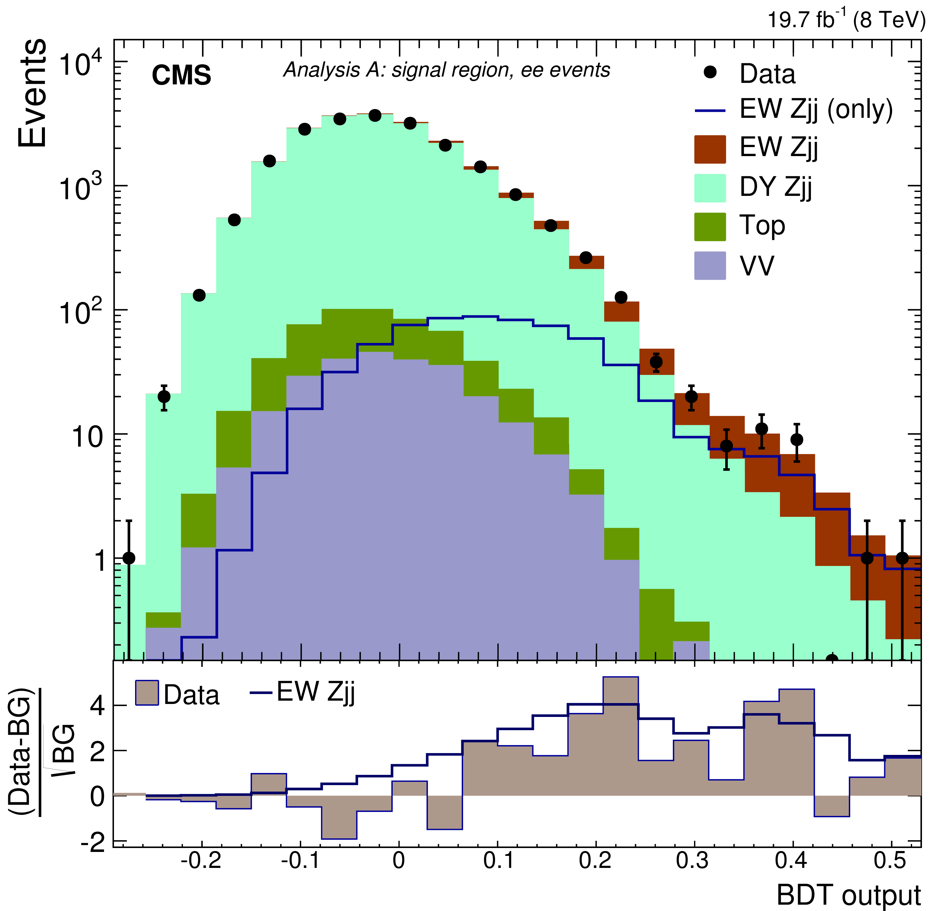
Figure 7-a:
Distributions for the BDT discriminants in ee (top row) and $\mu \mu $ (bottom row) events, used by analysis A. The distributions obtained in the control regions are shown at the left while the ones obtained in the signal region are shown at the right. The ratios for data to MC simulations are given in the bottom panels in the left column, showing the impact of changes in JES by $\pm $1 SD. The bottom panels of the right column show the differences between data or the expected ${\mathrm {EW} \mathrm{ Z } \mathrm {jj}} $ contribution with respect to the background (BG). |
png pdf |
Figure 7-b:
Distributions for the BDT discriminants in ee (top row) and $\mu \mu $ (bottom row) events, used by analysis A. The distributions obtained in the control regions are shown at the left while the ones obtained in the signal region are shown at the right. The ratios for data to MC simulations are given in the bottom panels in the left column, showing the impact of changes in JES by $\pm $1 SD. The bottom panels of the right column show the differences between data or the expected ${\mathrm {EW} \mathrm{ Z } \mathrm {jj}} $ contribution with respect to the background (BG). |

png pdf |
Figure 7-c:
Distributions for the BDT discriminants in ee (top row) and $\mu \mu $ (bottom row) events, used by analysis A. The distributions obtained in the control regions are shown at the left while the ones obtained in the signal region are shown at the right. The ratios for data to MC simulations are given in the bottom panels in the left column, showing the impact of changes in JES by $\pm $1 SD. The bottom panels of the right column show the differences between data or the expected ${\mathrm {EW} \mathrm{ Z } \mathrm {jj}} $ contribution with respect to the background (BG). |

png pdf |
Figure 7-d:
Distributions for the BDT discriminants in ee (top row) and $\mu \mu $ (bottom row) events, used by analysis A. The distributions obtained in the control regions are shown at the left while the ones obtained in the signal region are shown at the right. The ratios for data to MC simulations are given in the bottom panels in the left column, showing the impact of changes in JES by $\pm $1 SD. The bottom panels of the right column show the differences between data or the expected ${\mathrm {EW} \mathrm{ Z } \mathrm {jj}} $ contribution with respect to the background (BG). |

png pdf |
Figure 8-a:
Distributions for the BDT discriminants in $\mu \mu $ events, for the control region (left) and signal region (right), used by analysis B. The ratio for data to MC simulations is given in the bottom panel on the left, showing the impact of changes in JES by $\pm $1 SD. The bottom panel on the right shows the difference between data or the expected ${\mathrm {EW} \mathrm{ Z } \mathrm {jj}} $ contribution with respect to the background (BG). |

png pdf |
Figure 8-b:
Distributions for the BDT discriminants in $\mu \mu $ events, for the control region (left) and signal region (right), used by analysis B. The ratio for data to MC simulations is given in the bottom panel on the left, showing the impact of changes in JES by $\pm $1 SD. The bottom panel on the right shows the difference between data or the expected ${\mathrm {EW} \mathrm{ Z } \mathrm {jj}} $ contribution with respect to the background (BG). |
png pdf |
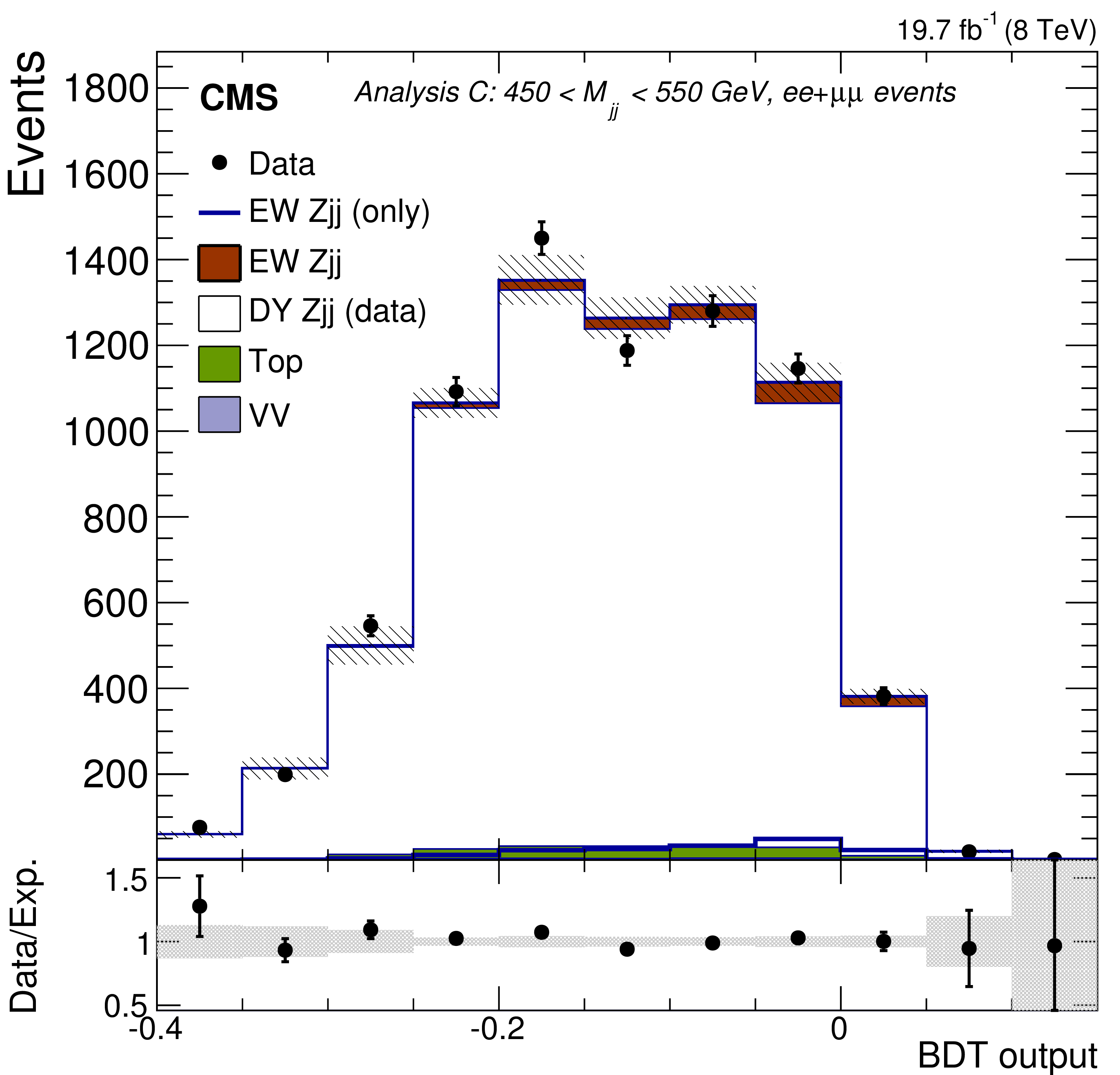
Figure 9-a:
Distributions for the BDT discriminants in ee+$\mu \mu $ events for different $M_\mathrm {jj}$ categories, used in analysis C. The ratios at the bottom each subfigure of the top row gives the results of data to expectation for the two control regions of $M_\mathrm {jj}$. The lower panel of the bottom subfigure shows the difference between data or the expected ${\mathrm {EW} \mathrm{ Z } \mathrm {jj}} $ contribution with respect to the background (BG). |

png pdf |
Figure 9-b:
Distributions for the BDT discriminants in ee+$\mu \mu $ events for different $M_\mathrm {jj}$ categories, used in analysis C. The ratios at the bottom each subfigure of the top row gives the results of data to expectation for the two control regions of $M_\mathrm {jj}$. The lower panel of the bottom subfigure shows the difference between data or the expected ${\mathrm {EW} \mathrm{ Z } \mathrm {jj}} $ contribution with respect to the background (BG). |
png pdf |
Figure 9-c:
Distributions for the BDT discriminants in ee+$\mu \mu $ events for different $M_\mathrm {jj}$ categories, used in analysis C. The ratios at the bottom each subfigure of the top row gives the results of data to expectation for the two control regions of $M_\mathrm {jj}$. The lower panel of the bottom subfigure shows the difference between data or the expected ${\mathrm {EW} \mathrm{ Z } \mathrm {jj}} $ contribution with respect to the background (BG). |

png pdf |
Figure 10:
Expected and observed contours for the 68% and 95% CL intervals on the ${\mathrm {EW} \mathrm{ Z } \mathrm {jj}} $ and DY signal strengths, obtained with method C after combination of the ee and $\mu \mu $ channels. |

png pdf |
Figure 11-a:
(left) The average number of jets with $ {p_{\mathrm {T}}} > $ 40 GeV as a function of the total $ {H_{\mathrm {T}}} $ in events containing a Z and at least one jet, and (right) average $\cos\Delta \phi _\mathrm {jj}$ as a function of the total $ {H_{\mathrm {T}}} $ in events containing a Z and at least two jets. The ratios of data to expectation are given below the main panels. At each ordinate, the entries are separated for clarity. The expectations for ${\mathrm {EW} \mathrm{ Z } \mathrm {jj}} $ are shown separately. The data and simulation points are shown with their statistical uncertainties. |
png pdf |
Figure 11-b:
(left) The average number of jets with $ {p_{\mathrm {T}}} > $ 40 GeV as a function of the total $ {H_{\mathrm {T}}} $ in events containing a Z and at least one jet, and (right) average $\cos\Delta \phi _\mathrm {jj}$ as a function of the total $ {H_{\mathrm {T}}} $ in events containing a Z and at least two jets. The ratios of data to expectation are given below the main panels. At each ordinate, the entries are separated for clarity. The expectations for ${\mathrm {EW} \mathrm{ Z } \mathrm {jj}} $ are shown separately. The data and simulation points are shown with their statistical uncertainties. |

png pdf |
Figure 12-a:
(left) The average number of jets with $ {p_{\mathrm {T}}} > $ 40 GeV as a function of the pseudorapidity distance between the dijet with largest $\Delta \eta $, and (right) average $\cos\Delta \phi _\mathrm {jj}$ as a function of $\Delta \eta _\mathrm {jj}$ between the dijet with largest $\Delta \eta $. In both cases events containing a Z and at least two jets are used. The ratios of data to expectation are given below the main panels. At each ordinate, the entries are separated for clarity. The expectations for ${\mathrm {EW} \mathrm{ Z } \mathrm {jj}} $ are shown separately. The data and simulation points are shown with their statistical uncertainties. |
png pdf |
Figure 12-b:
(left) The average number of jets with $ {p_{\mathrm {T}}} > $ 40 GeV as a function of the pseudorapidity distance between the dijet with largest $\Delta \eta $, and (right) average $\cos\Delta \phi _\mathrm {jj}$ as a function of $\Delta \eta _\mathrm {jj}$ between the dijet with largest $\Delta \eta $. In both cases events containing a Z and at least two jets are used. The ratios of data to expectation are given below the main panels. At each ordinate, the entries are separated for clarity. The expectations for ${\mathrm {EW} \mathrm{ Z } \mathrm {jj}} $ are shown separately. The data and simulation points are shown with their statistical uncertainties. |

png pdf |
Figure 13-a:
Average soft $ {H_{\mathrm {T}}} $ computed using the three leading soft-track jets reconstructed in the $\Delta \eta _\mathrm {jj}$ pseudorapidity interval between the tagging jets that have $ {p_{\mathrm {T}}} > $ 50 GeV and $ {p_{\mathrm {T}}} > $ 30 GeV. The average soft $ {H_{\mathrm {T}}} $ is shown as function of: (left) $M_\mathrm {jj}$ and (right) $\Delta \eta _\mathrm {jj}$ for both the dielectron and dimuon channels. The ratios of data to expectation are given below the main panels. At each ordinate, the entries are separated for clarity. The expectations for ${\mathrm {EW} \mathrm{ Z } \mathrm {jj}} $ are shown separately. The data and simulation points are shown with their statistical uncertainties. |
png pdf |
Figure 13-b:
Average soft $ {H_{\mathrm {T}}} $ computed using the three leading soft-track jets reconstructed in the $\Delta \eta _\mathrm {jj}$ pseudorapidity interval between the tagging jets that have $ {p_{\mathrm {T}}} > $ 50 GeV and $ {p_{\mathrm {T}}} > $ 30 GeV. The average soft $ {H_{\mathrm {T}}} $ is shown as function of: (left) $M_\mathrm {jj}$ and (right) $\Delta \eta _\mathrm {jj}$ for both the dielectron and dimuon channels. The ratios of data to expectation are given below the main panels. At each ordinate, the entries are separated for clarity. The expectations for ${\mathrm {EW} \mathrm{ Z } \mathrm {jj}} $ are shown separately. The data and simulation points are shown with their statistical uncertainties. |
png pdf |
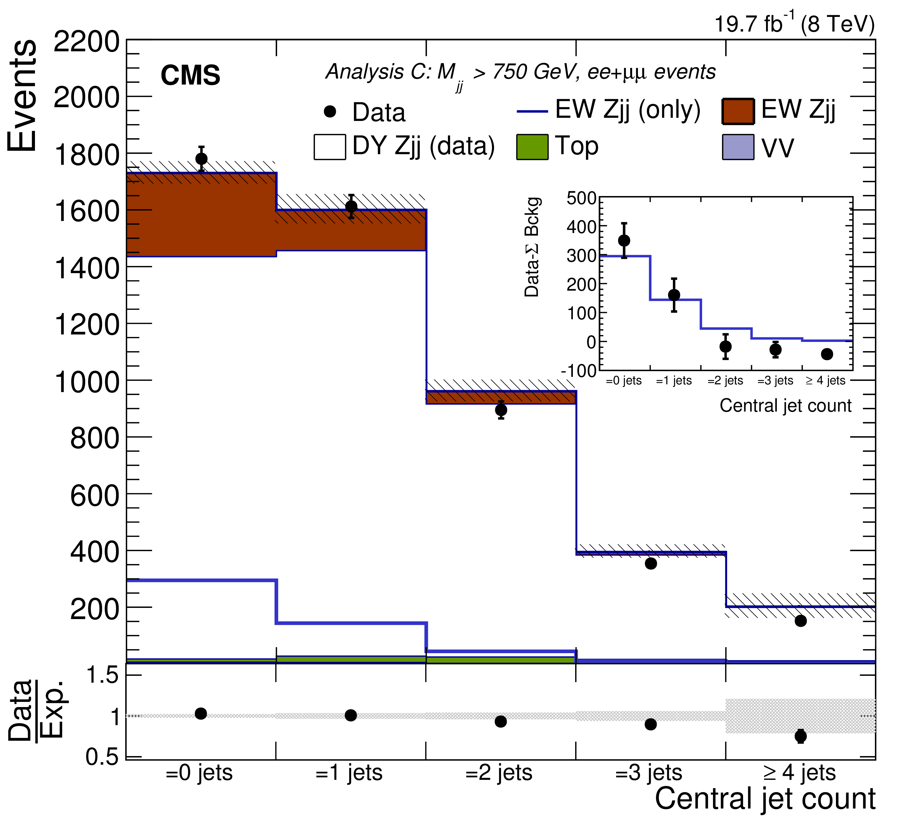
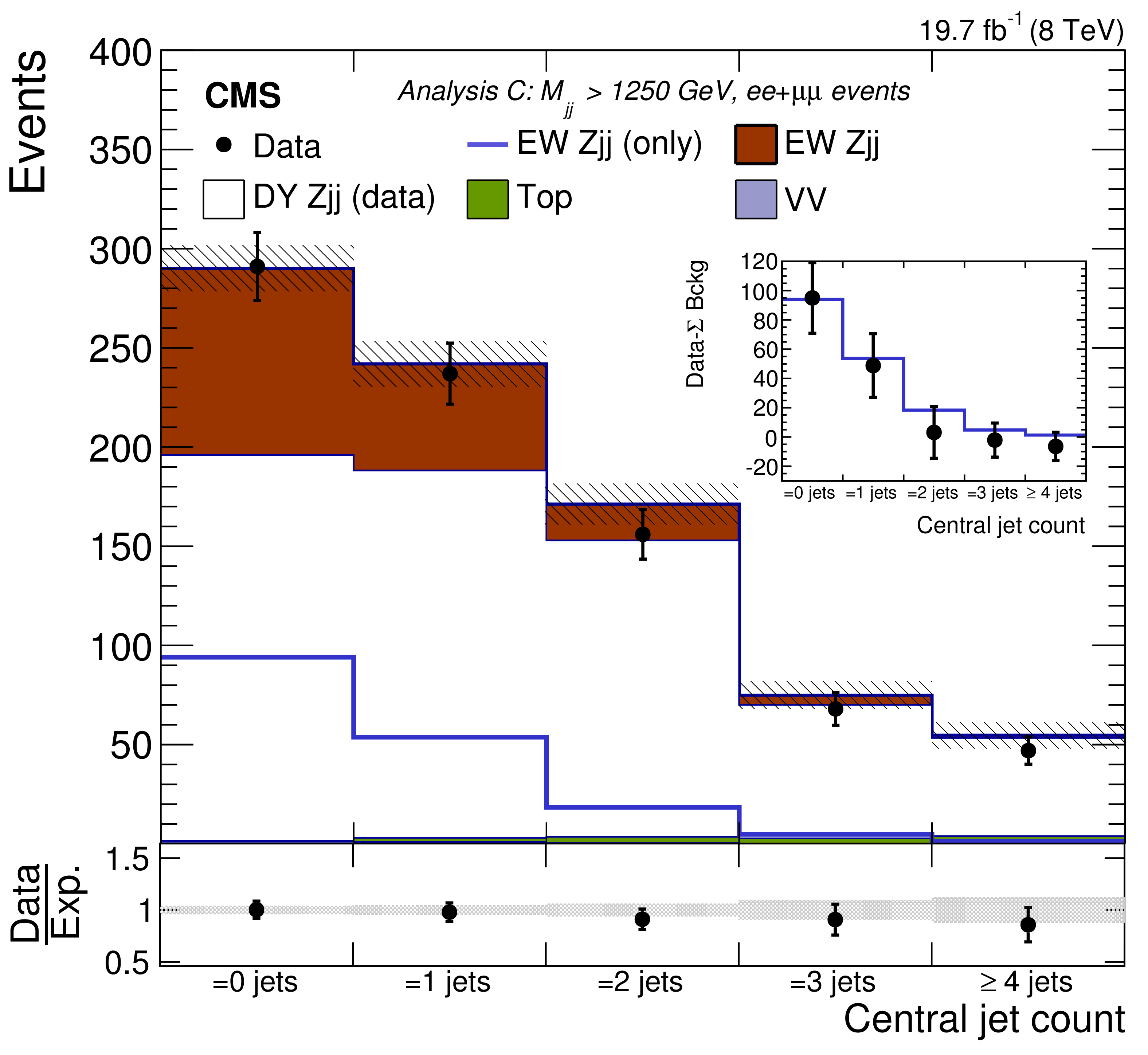
Figure 14-a:
Additional jet multiplicity (top row), and corresponding $ {H_{\mathrm {T}}} $ (bottom row) within the $\Delta \eta _{\mathrm {jj}}$ of the two tagging jets in events with $M_\mathrm {jj}> $ 750 GeV (left column) or $M_\mathrm {jj}> $ 1250 GeV (right column). In the main panels the expected contributions from ${\mathrm {EW} \mathrm{ Z } \mathrm {jj}} $, ${\mathrm {DY} \mathrm{ Z } \mathrm {jj}} $, and residual backgrounds are shown stacked, and compared to the observed data. The signal-only contribution is superimposed separately and it is also compared to the residual data after the subtraction of the expected backgrounds in the insets. The ratio of data to expectation is represented by point markers in the bottom panels. The total uncertainties assigned to the expectations are represented as shaded bands. |
png pdf |
Figure 14-b:
Additional jet multiplicity (top row), and corresponding $ {H_{\mathrm {T}}} $ (bottom row) within the $\Delta \eta _{\mathrm {jj}}$ of the two tagging jets in events with $M_\mathrm {jj}> $ 750 GeV (left column) or $M_\mathrm {jj}> $ 1250 GeV (right column). In the main panels the expected contributions from ${\mathrm {EW} \mathrm{ Z } \mathrm {jj}} $, ${\mathrm {DY} \mathrm{ Z } \mathrm {jj}} $, and residual backgrounds are shown stacked, and compared to the observed data. The signal-only contribution is superimposed separately and it is also compared to the residual data after the subtraction of the expected backgrounds in the insets. The ratio of data to expectation is represented by point markers in the bottom panels. The total uncertainties assigned to the expectations are represented as shaded bands. |

png pdf |
Figure 14-c:
Additional jet multiplicity (top row), and corresponding $ {H_{\mathrm {T}}} $ (bottom row) within the $\Delta \eta _{\mathrm {jj}}$ of the two tagging jets in events with $M_\mathrm {jj}> $ 750 GeV (left column) or $M_\mathrm {jj}> $ 1250 GeV (right column). In the main panels the expected contributions from ${\mathrm {EW} \mathrm{ Z } \mathrm {jj}} $, ${\mathrm {DY} \mathrm{ Z } \mathrm {jj}} $, and residual backgrounds are shown stacked, and compared to the observed data. The signal-only contribution is superimposed separately and it is also compared to the residual data after the subtraction of the expected backgrounds in the insets. The ratio of data to expectation is represented by point markers in the bottom panels. The total uncertainties assigned to the expectations are represented as shaded bands. |

png pdf |
Figure 14-d:
Additional jet multiplicity (top row), and corresponding $ {H_{\mathrm {T}}} $ (bottom row) within the $\Delta \eta _{\mathrm {jj}}$ of the two tagging jets in events with $M_\mathrm {jj}> $ 750 GeV (left column) or $M_\mathrm {jj}> $ 1250 GeV (right column). In the main panels the expected contributions from ${\mathrm {EW} \mathrm{ Z } \mathrm {jj}} $, ${\mathrm {DY} \mathrm{ Z } \mathrm {jj}} $, and residual backgrounds are shown stacked, and compared to the observed data. The signal-only contribution is superimposed separately and it is also compared to the residual data after the subtraction of the expected backgrounds in the insets. The ratio of data to expectation is represented by point markers in the bottom panels. The total uncertainties assigned to the expectations are represented as shaded bands. |

png pdf |
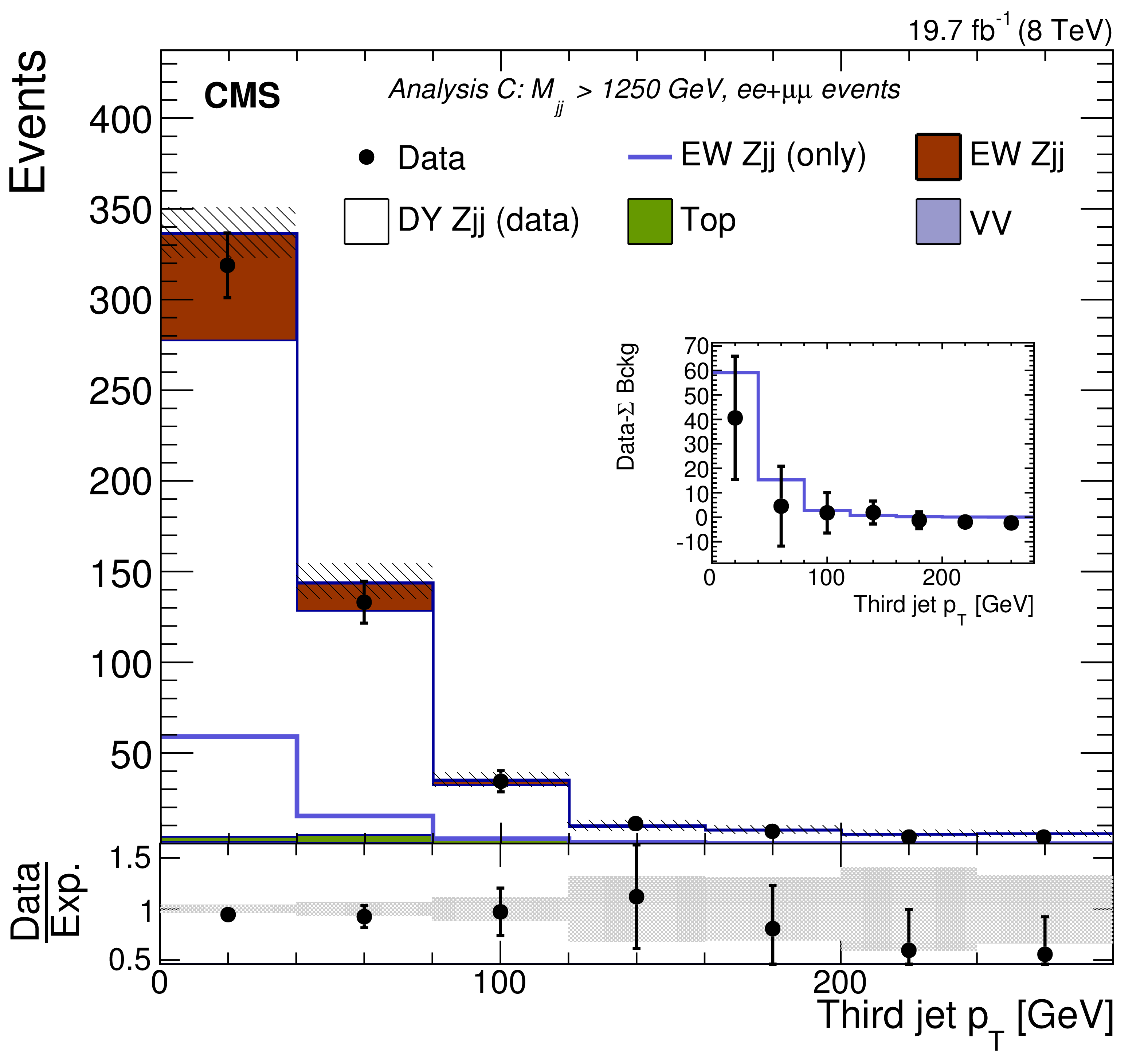
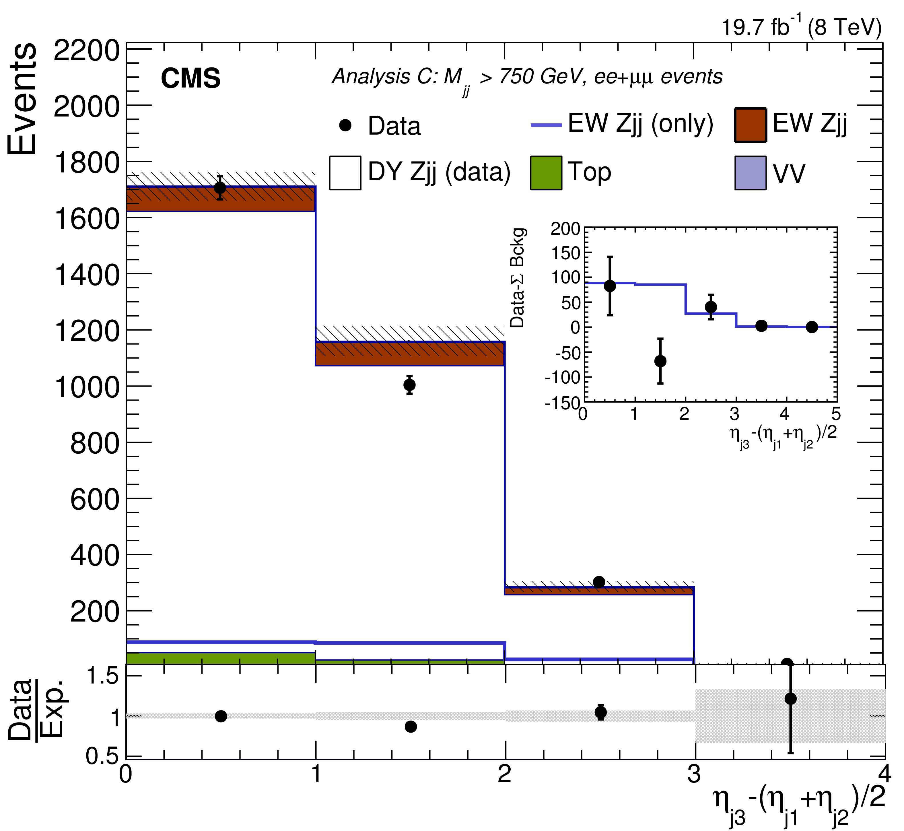
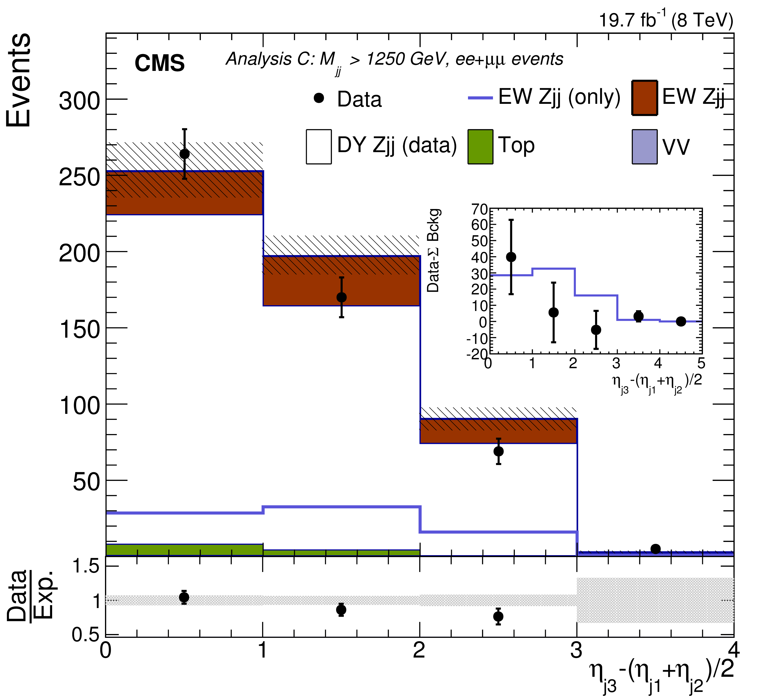
Figure 15-a:
(top row) ${p_{\mathrm {T}}}$ and (bottom row) $\eta ^*_{\mathrm {j}3}$ of the leading additional jet within the $\Delta \eta _{\mathrm {jj}}$ of the two tagging jets in events with $M_\mathrm {jj}> $ 750 GeV (left column) or $M_\mathrm {jj}> $ 1250 GeV (right column). The explanation of the plots is similar to Fig. 14. |
png pdf |
Figure 15-b:
(top row) ${p_{\mathrm {T}}}$ and (bottom row) $\eta ^*_{\mathrm {j}3}$ of the leading additional jet within the $\Delta \eta _{\mathrm {jj}}$ of the two tagging jets in events with $M_\mathrm {jj}> $ 750 GeV (left column) or $M_\mathrm {jj}> $ 1250 GeV (right column). The explanation of the plots is similar to Fig. 14. |
png pdf |
Figure 15-c:
(top row) ${p_{\mathrm {T}}}$ and (bottom row) $\eta ^*_{\mathrm {j}3}$ of the leading additional jet within the $\Delta \eta _{\mathrm {jj}}$ of the two tagging jets in events with $M_\mathrm {jj}> $ 750 GeV (left column) or $M_\mathrm {jj}> $ 1250 GeV (right column). The explanation of the plots is similar to Fig. 14. |
png pdf |
Figure 15-d:
(top row) ${p_{\mathrm {T}}}$ and (bottom row) $\eta ^*_{\mathrm {j}3}$ of the leading additional jet within the $\Delta \eta _{\mathrm {jj}}$ of the two tagging jets in events with $M_\mathrm {jj}> $ 750 GeV (left column) or $M_\mathrm {jj}> $ 1250 GeV (right column). The explanation of the plots is similar to Fig. 14. |

png pdf |
Figure 16-a:
Gap fractions for: (top row) ${p_{\mathrm {T}}}$ of leading additional jet, (bottom row) the $ {H_{\mathrm {T}}} $ variable within the $\Delta \eta _{\mathrm {jj}}$ of the two tagging jets in events with $M_\mathrm {jj}> $ 750 GeV (left) or $M_\mathrm {jj}> $ 1250 GeV (right). The observed gap fractions in data are compared to two different signal plus background predictions where ${\mathrm {DY} \mathrm{ Z } \mathrm {jj}} $ is modelled either from ${\gamma \mathrm {jj}} $ data or from simulation. The bottom panels show the ratio between the observed data and different predictions. |

png pdf |
Figure 16-b:
Gap fractions for: (top row) ${p_{\mathrm {T}}}$ of leading additional jet, (bottom row) the $ {H_{\mathrm {T}}} $ variable within the $\Delta \eta _{\mathrm {jj}}$ of the two tagging jets in events with $M_\mathrm {jj}> $ 750 GeV (left) or $M_\mathrm {jj}> $ 1250 GeV (right). The observed gap fractions in data are compared to two different signal plus background predictions where ${\mathrm {DY} \mathrm{ Z } \mathrm {jj}} $ is modelled either from ${\gamma \mathrm {jj}} $ data or from simulation. The bottom panels show the ratio between the observed data and different predictions. |

png pdf |
Figure 16-c:
Gap fractions for: (top row) ${p_{\mathrm {T}}}$ of leading additional jet, (bottom row) the $ {H_{\mathrm {T}}} $ variable within the $\Delta \eta _{\mathrm {jj}}$ of the two tagging jets in events with $M_\mathrm {jj}> $ 750 GeV (left) or $M_\mathrm {jj}> $ 1250 GeV (right). The observed gap fractions in data are compared to two different signal plus background predictions where ${\mathrm {DY} \mathrm{ Z } \mathrm {jj}} $ is modelled either from ${\gamma \mathrm {jj}} $ data or from simulation. The bottom panels show the ratio between the observed data and different predictions. |

png pdf |
Figure 16-d:
Gap fractions for: (top row) ${p_{\mathrm {T}}}$ of leading additional jet, (bottom row) the $ {H_{\mathrm {T}}} $ variable within the $\Delta \eta _{\mathrm {jj}}$ of the two tagging jets in events with $M_\mathrm {jj}> $ 750 GeV (left) or $M_\mathrm {jj}> $ 1250 GeV (right). The observed gap fractions in data are compared to two different signal plus background predictions where ${\mathrm {DY} \mathrm{ Z } \mathrm {jj}} $ is modelled either from ${\gamma \mathrm {jj}} $ data or from simulation. The bottom panels show the ratio between the observed data and different predictions. |
| Tables | |
png pdf |
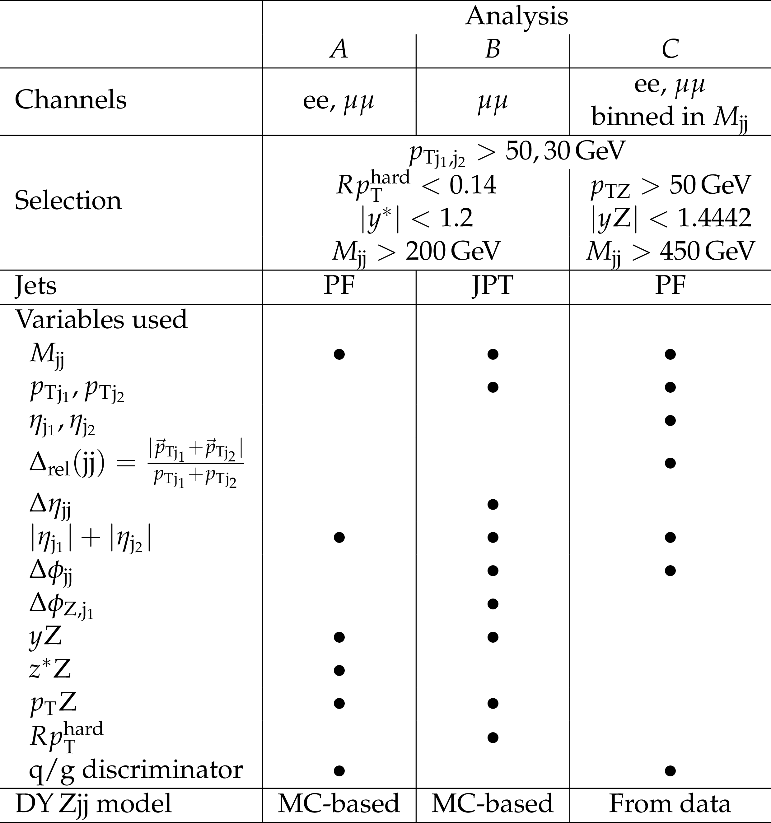
Table 1:
Comparison of the selections and variables used in three different analyses. The variables marked with the black circle are used in the discriminant of the indicated analysis. |
png pdf |
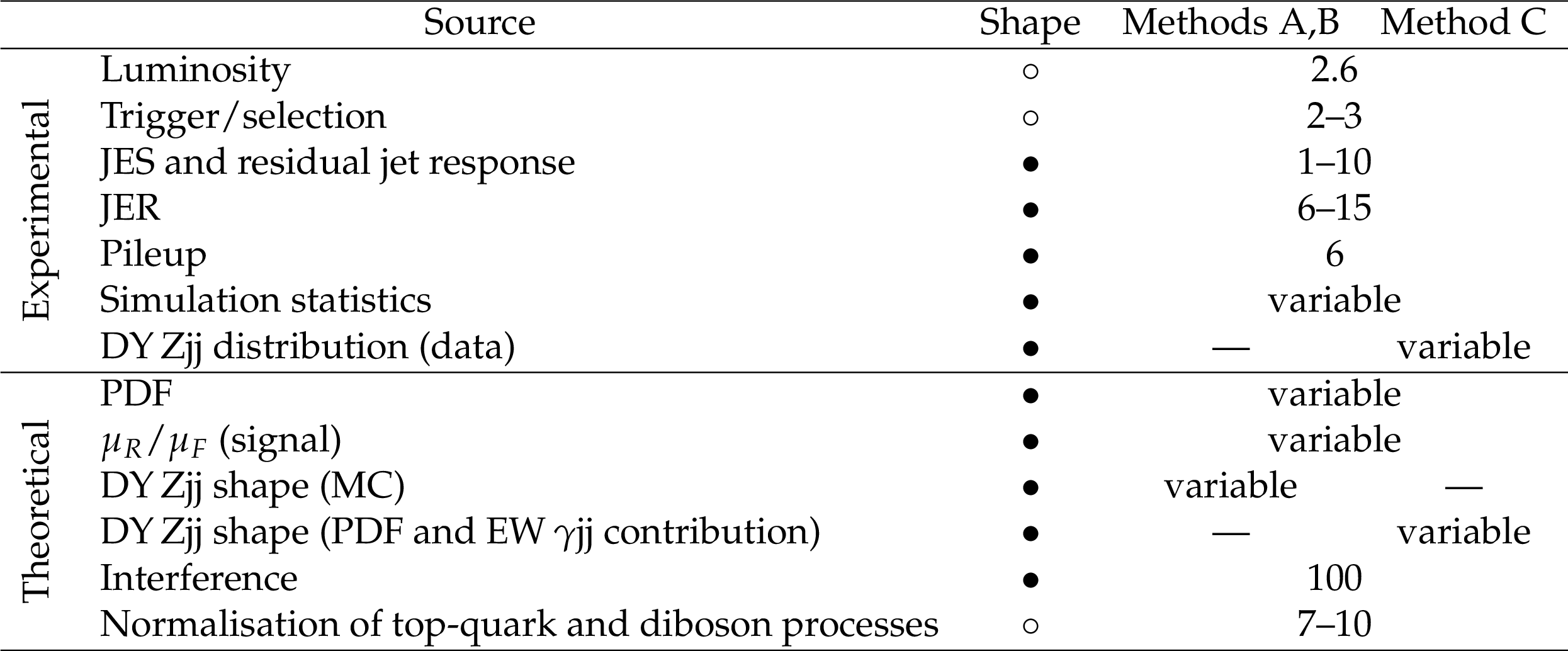
Table 2:
Summary of the relative variation of uncertainty sources (in %) considered for the evaluation of the systematic uncertainties in the different analyses. A filled or open circle signals whether that uncertainty affects the distribution or the absolute rate of a process in the fit, respectively. For some of the uncertainty sources ``variable'' is used to signal that the range is not unambiguously quantifiable by a range, as it depends on the value of the discriminants, event category and may also have a statistical component. |

png pdf |
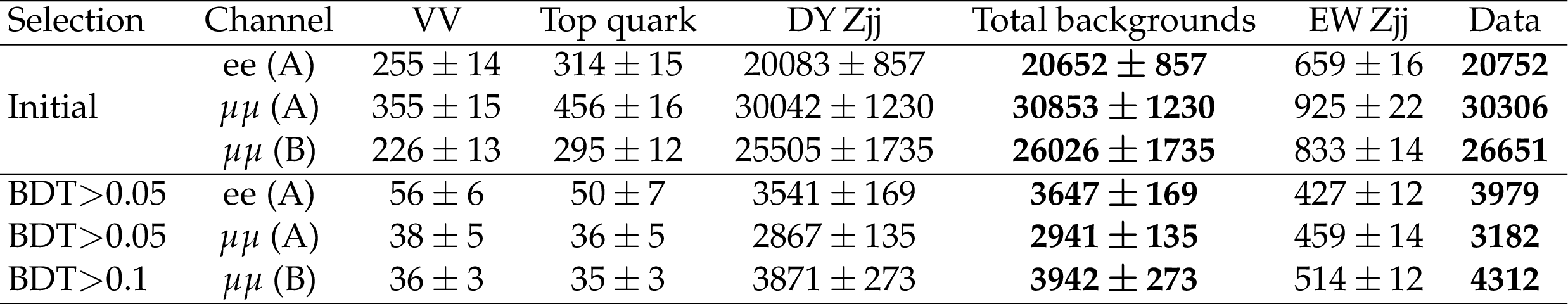
Table 3:
Event yields expected after fits to background and signal processes in methods A or B, using the initial selections (summarised in Table {tab:methodcomp}), and requiring ${S/B}>10\%$. The yields are compared to the data observed in the different channels and categories. The total uncertainties quoted for signal, ${\mathrm {DY} \mathrm{ Z } \mathrm {jj}} $, dibosons (VV), and processes with top quarks ($ {\mathrm{ t \bar{t} } }$ and single top quarks) are dominated by JES uncertainties and include other sources, e.g., the statistical fluctuations in the MC samples . |
png pdf |
Table 4:
Event yields expected before the fit to background and signal processes in method C. The yields are compared to the data observed in the different channels and categories. The total systematic uncertainty assigned to the normalisation of the processes is shown. |
png pdf |
Table 5:
Fitted signal strengths in the different analyses and channels including the statistical and systematic uncertainties. For method C, only events with $M_\mathrm {jj}> $ 450 GeV are used. The breakup of the systematic components of the uncertainty is given in detail in the listings. |
| Summary |
| The cross section for the purely electroweak production of a Z boson in association with two jets in the $\ell\ell j j $ final state, in proton-proton collisions at $ \sqrt{s} = $ 8 TeV has been measured. |
| References | ||||
| 1 | C. Oleari and D. Zeppenfeld | QCD corrections to electroweak $ \ell\nu_\ell $jj and $ \ell^+\ell^- $jj production | PRD 69 (2004) 093004 | hep-ph/0310156 |
| 2 | D. L. Rainwater, R. Szalapski, and D. Zeppenfeld | Probing color-singlet exchange in Z + 2 jet events at the CERN LHC | PRD 54 (1996) 6680 | hep-ph/9605444 |
| 3 | V. A. Khoze, M. G. Ryskin, W. J. Stirling, and P. H. Williams | A Z-monitor to calibrate Higgs production via vector boson fusion with rapidity gaps at the LHC | EPJC 26 (2003) 429 | hep-ph/0207365 |
| 4 | ATLAS Collaboration | Observation of a new particle in the search for the Standard Model Higgs boson with the ATLAS detector at the LHC | PLB 716 (2012) 1 | 1207.7214 |
| 5 | CMS Collaboration | Observation of a new boson at a mass of 125 GeV with the CMS experiment at the LHC | PLB 716 (2012) 30 | CMS-HIG-12-028 1207.7235 |
| 6 | CMS Collaboration | Observation of a new boson with mass near 125 GeV in pp collisions at $ \sqrt{s} $ = 7 and 8 TeV | JHEP 06 (2013) 081 | CMS-HIG-12-036 1303.4571 |
| 7 | G.-C. Cho et al. | Weak boson fusion production of supersymmetric particles at the CERN LHC | PRD 73 (2006) 054002 | hep-ph/0601063 |
| 8 | B. Dutta et al. | Vector boson fusion processes as a probe of supersymmetric electroweak sectors at the LHC | PRD 87 (2013) 035029 | 1210.0964 |
| 9 | J. D. Bjorken | Rapidity gaps and jets as a new physics signature in very high-energy hadron hadron collisions | PRD 47 (1993) 101 | |
| 10 | F. Schissler and D. Zeppenfeld | Parton shower effects on W and Z production via vector boson fusion at NLO QCD | JHEP 04 (2013) 057 | 1302.2884 |
| 11 | CMS Collaboration | Measurement of the hadronic activity in events with a Z and two jets and extraction of the cross section for the electroweak production of a Z with two jets in pp collisions at $ \sqrt{s} $ = 7 TeV | JHEP 10 (2013) 062 | CMS-FSQ-12-019 1305.7389 |
| 12 | ATLAS Collaboration | Measurement of the electroweak production of dijets in association with a Z-boson and distributions sensitive to vector boson fusion in proton-proton collisions at $ \sqrt{s} $ = 8 TeV using the ATLAS detector | JHEP 04 (2014) 031 | 1401.7610 |
| 13 | CMS Collaboration | Energy calibration and resolution of the CMS electromagnetic calorimeter in pp collisions at $ \sqrt{s} $ = 7 TeV | JINST 8 (2013) P09009 | CMS-EGM-11-001 1306.2016 |
| 14 | CMS Collaboration | Determination of jet energy calibration and transverse momentum resolution in CMS | JINST 6 (2011) P11002 | CMS-JME-10-011 1107.4277 |
| 15 | J. Alwall et al. | MadGraph 5: going beyond | JHEP 06 (2011) 128 | 1106.0522 |
| 16 | J. Alwall et al. | The automated computation of tree-level and next-to-leading order differential cross sections, and their matching to parton shower simulations | JHEP 07 (2014) 079 | 1405.0301 |
| 17 | T. Sj\"ostrand, S. Mrenna, and P. Z. Skands | PYTHIA 6.4 physics and manual | JHEP 05 (2006) 026 | hep-ph/0603175 |
| 18 | J. Pumplin et al. | New generation of parton distributions with uncertainties from global QCD analysis | JHEP 07 (2002) 012 | hep-ph/0201195 |
| 19 | Particle Data Group, J. Beringer et al. | Review of Particle Physics | PRD 86 (2012) 010001 | |
| 20 | CMS Collaboration | Measurement of the Underlying Event Activity at the LHC with $ \sqrt{s} $ = 7 TeV and Comparison with $ \sqrt{s} $ = 0.9 TeV | JHEP 09 (2011) 109 | CMS-QCD-10-010 1107.0330 |
| 21 | S. Alekhin et al. | The PDF4LHC Working Group Interim Report | 1101.0536 | |
| 22 | M. Botje et al. | The PDF4LHC Working Group Interim Recommendations | 1101.0538 | |
| 23 | NNPDF Collaboration | A first unbiased global NLO determination of parton distributions and their uncertainties | Nucl. Phys. B 838 (2010) 136 | 1002.4407 |
| 24 | A. D. Martin, W. J. Stirling, R. S. Thorne, and G. Watt | Parton distributions for the LHC | EPJC 63 (2009) 189 | 0901.0002 |
| 25 | K. Arnold et al. | VBFNLO: A parton level Monte Carlo for processes with electroweak bosons | CPC 180 (2009) 1661 | 0811.4559 |
| 26 | J. Baglio et al. | VBFNLO: a parton level Monte Carlo for processes with electroweak bosons --- manual for version 2.7.0 | 1107.4038 | |
| 27 | K. Arnold et al. | Release Note -- VBFNLO-2.6.0 | 1207.4975 | |
| 28 | M. L. Mangano, M. Moretti, F. Piccinini, and M. Treccani | Matching matrix elements and shower evolution for top-quark production in hadronic collisions | JHEP 01 (2007) 013 | hep-ph/0611129 |
| 29 | J. Alwall et al. | Comparative study of various algorithms for the merging of parton showers and matrix elements in hadronic collisions | EPJC 53 (2008) 473 | 0706.2569 |
| 30 | K. Melnikov and F. Petriello | Electroweak gauge boson production at hadron colliders through $ O(\alpha_S^2) $ | PRD 74 (2006) 114017 | hep-ph/0609070 |
| 31 | M. Czakon, P. Fiedler, and A. Mitov | The total top quark pair production cross-section at hadron colliders through $ \mathcal{O}(\alpha_S^4) $ | PRL 110 (2013) 252004 | 1303.6254 |
| 32 | S. Alioli, P. Nason, C. Oleari, and E. Re | A general framework for implementing NLO calculations in shower Monte Carlo programs: the POWHEG BOX | JHEP 06 (2010) 043 | 1002.2581 |
| 33 | P. Nason | A new method for combining NLO QCD with shower Monte Carlo algorithms | JHEP 11 (2004) 040 | hep-ph/0409146 |
| 34 | S. Frixione, P. Nason, and C. Oleari | Matching NLO QCD computations with parton shower simulations: the POWHEG method | JHEP 11 (2007) 070 | 0709.2092 |
| 35 | S. Alioli, P. Nason, C. Oleari, and E. Re | NLO single-top production matched with shower in POWHEG: $ \it $ s- and $ \it $ t-channel contributions | JHEP 09 (2009) 111, , [Erratum: \DOI10.1007/JHEP02(2010)011] | 0907.4076 |
| 36 | E. Re | Single-top $ \it $ Wt-channel production matched with parton showers using the POWHEG method | EPJC 71 (2011) 1547 | 1009.2450 |
| 37 | N. Kidonakis | Differential and total cross sections for top pair and single top production | in Proceedings of the XX International Workshop on Deep-Inelastic Scattering and Related Subjects Bonn, Germany | 1205.3453 |
| 38 | N. Kidonakis | Top Quark Production | 1311.0283 | |
| 39 | T. Gehrmann et al. | $ \mathrm{ W }p\mathrm{ W }m $ production at hadron colliders in NNLO QCD | 1408.5243 | |
| 40 | J. M. Campbell and R. K. Ellis | MCFM for the Tevatron and the LHC | Nucl. Phys. B Proc. Suppl. 205-206 (2010) 10 | 1007.3492 |
| 41 | J. Allison et al. | Geant4 developments and applications | IEEE Trans. Nucl. Sci. 53 (2006) 270 | |
| 42 | GEANT4 Collaboration | GEANT4---a simulation toolkit | NIMA 506 (2003) 250 | |
| 43 | CMS Collaboration | Electron Reconstruction and Identification at $ \sqrt{s} $ = 7 TeV | CDS | |
| 44 | CMS Collaboration | Performance of CMS muon reconstruction in pp collision events at $ \sqrt{s} $ = 7 TeV | JINST 7 (2012) P10002 | CMS-MUO-10-004 1206.4071 |
| 45 | CMS Collaboration | The CMS experiment at the CERN LHC | JINST 3 (2008) S08004 | CMS-00-001 |
| 46 | CMS Collaboration | Jet Plus Tracks Algorithm for Calorimeter Jet Energy Corrections in CMS | CDS | |
| 47 | M. Cacciari, G. P. Salam, and G. Soyez | The anti-$ k_t $ jet clustering algorithm | JHEP 04 (2008) 063 | 0802.1189 |
| 48 | M. Cacciari, G. P. Salam, and G. Soyez | FastJet user manual | EPJC 72 (2012) 1896 | 1111.6097 |
| 49 | CMS Collaboration | Particle--Flow Event Reconstruction in CMS and Performance for Jets, Taus, and $ E_{\mathrm{T}}^{\text{miss}} $ | CDS | |
| 50 | CMS Collaboration | Commissioning of the particle-flow Event Reconstruction with the first LHC collisions recorded in the CMS detector | CDS | |
| 51 | M. Cacciari and G. P. Salam | Pileup subtraction using jet areas | PLB 659 (2008) 119 | 0707.1378 |
| 52 | M. Cacciari, G. P. Salam, and G. Soyez | The catchment area of jets | JHEP 04 (2008) 005 | 0802.1188 |
|
|
Compact Muon Solenoid LHC, CERN |
|

|

|

|

|

|