CMS-HIG-13-012

CMS-HIG-13-012 ; CERN-PH-EP-2013-188
Search for the standard model Higgs boson produced in association with a W or a Z boson and decaying to bottom quarks
CMS Collaboration
14 October 2013
Phys. Rev. D 89 (2014) 012003
Abstract: A search for the standard model Higgs boson (H) decaying to $ \mathrm{b \bar{b} } $ when produced in association with a weak vector boson (V) is reported for the following channels: W($ \mu \nu $)H, W($ \mathrm{e} \nu $)H, W($ \tau \nu $)H, Z($ \mu \mu $)H, Z($ \mathrm{ e e } $)H, and Z($ \nu \nu $)H. The search is performed in data samples corresponding to integrated luminosities of up to 5.1 fb$ ^{-1} $ at $ \sqrt{s} $ = 7 TeV and up to 18.9 fb$ ^{-1} $ at $ \sqrt{s} $ = 8 TeV, recorded by the CMS experiment at the LHC. An excess of events is observed above the expected background with a local significance of 2.1 standard deviations for a Higgs boson mass of 125 GeV, consistent with the expectation from the production of the standard model Higgs boson. The signal strength corresponding to this excess, relative to that of the standard model Higgs boson, is 1.0 $ \pm $ 0.5.
Links: e-print arXiv:1310.3687 [hep-ex] (PDF) ; CDS record ; inSPIRE record ; Public twiki page ; CADI line (restricted) ;

Figures	CMS Publications

Figures
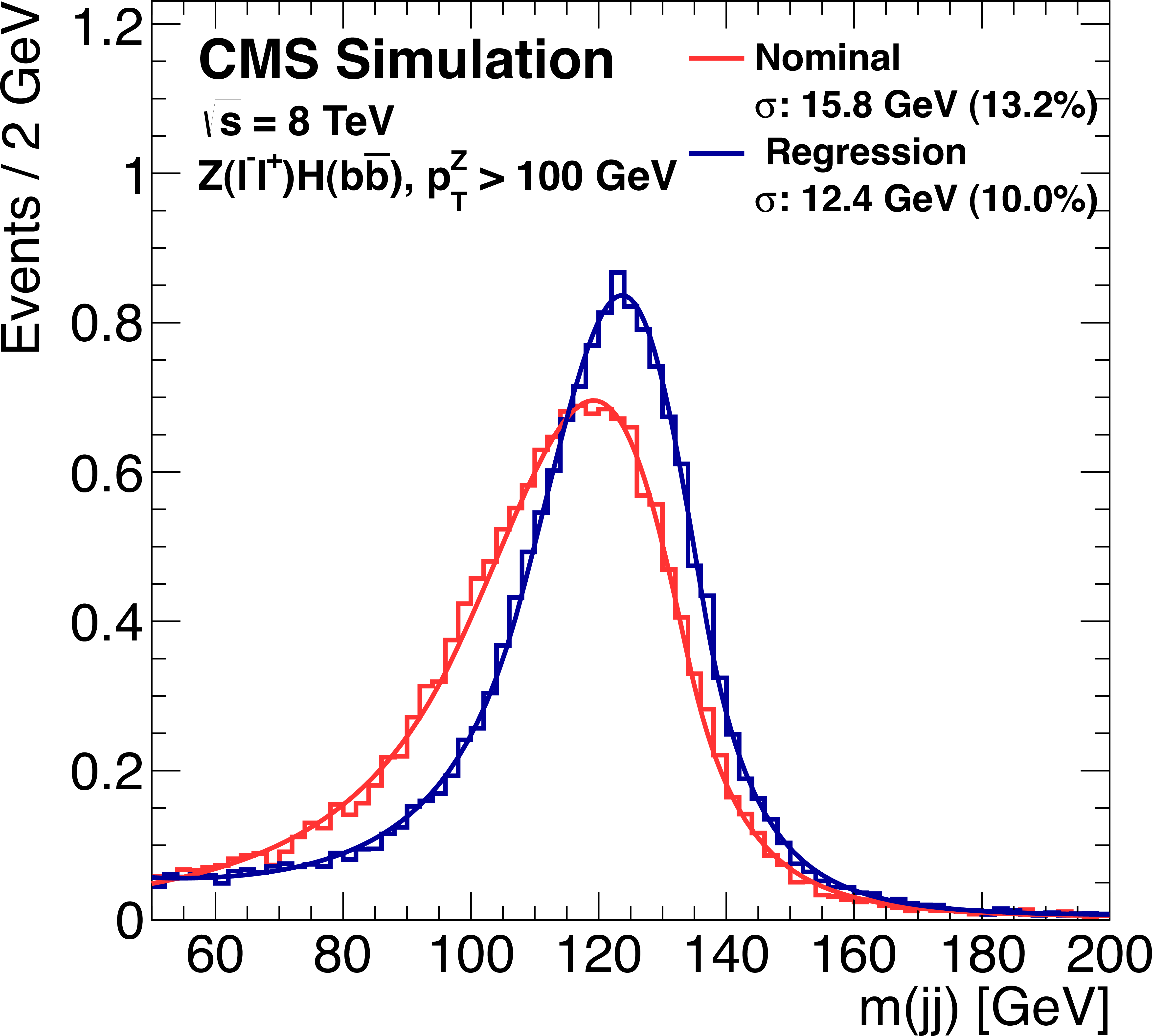
png pdf	Figure 1: Dijet invariant mass distribution for simulated samples of ${ {\mathrm {Z}}(\ell \ell ) {\mathrm {H}} ( {\mathrm {b}} {\mathrm {b}})}$ events ($m_{H}$ = 125 GeV), before (red) and after (blue) the energy correction from the regression procedure is applied. A Bukin function is fit to the distribution and the fitted width of the core of the distribution is displayed on the figure.
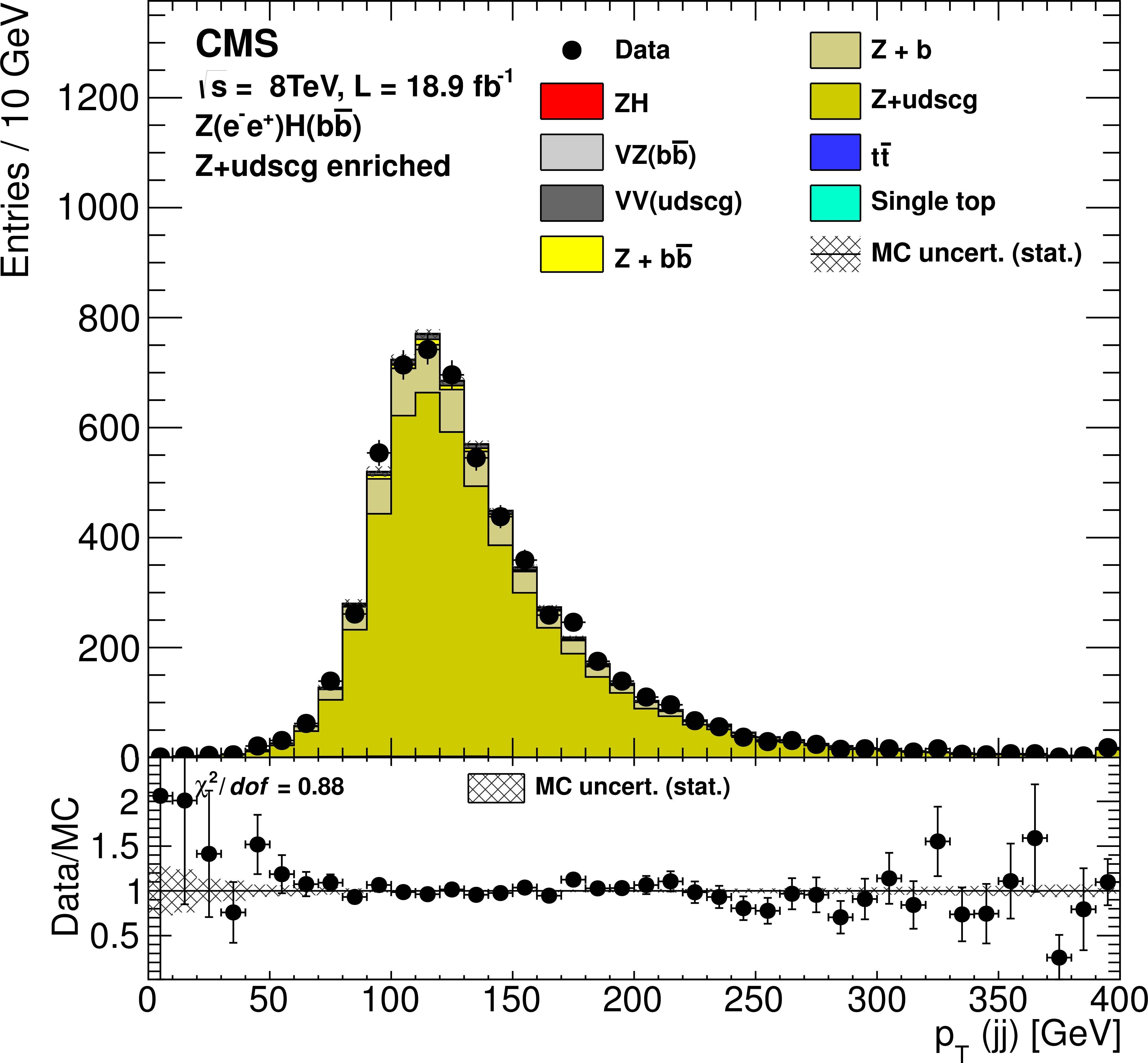
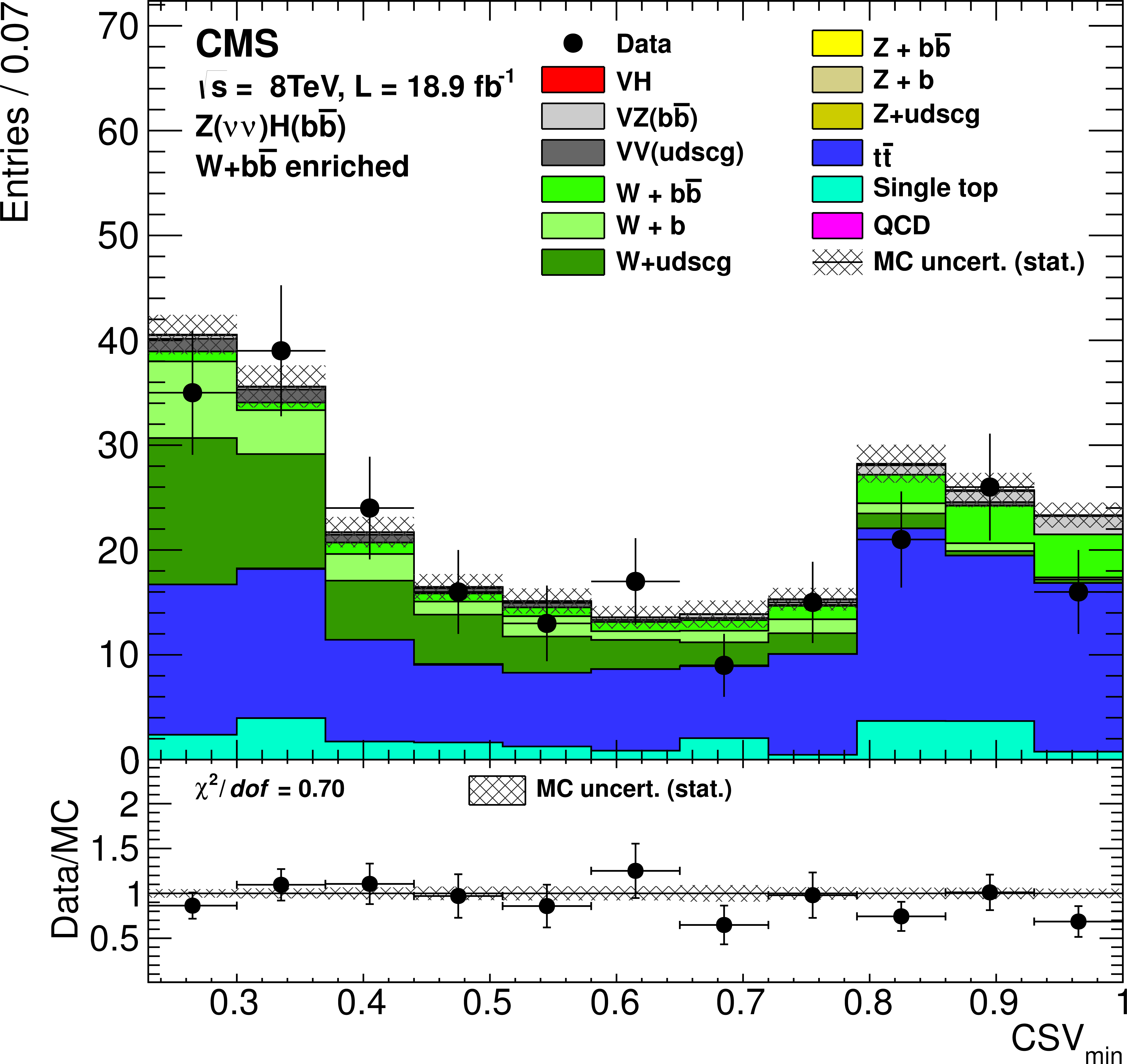
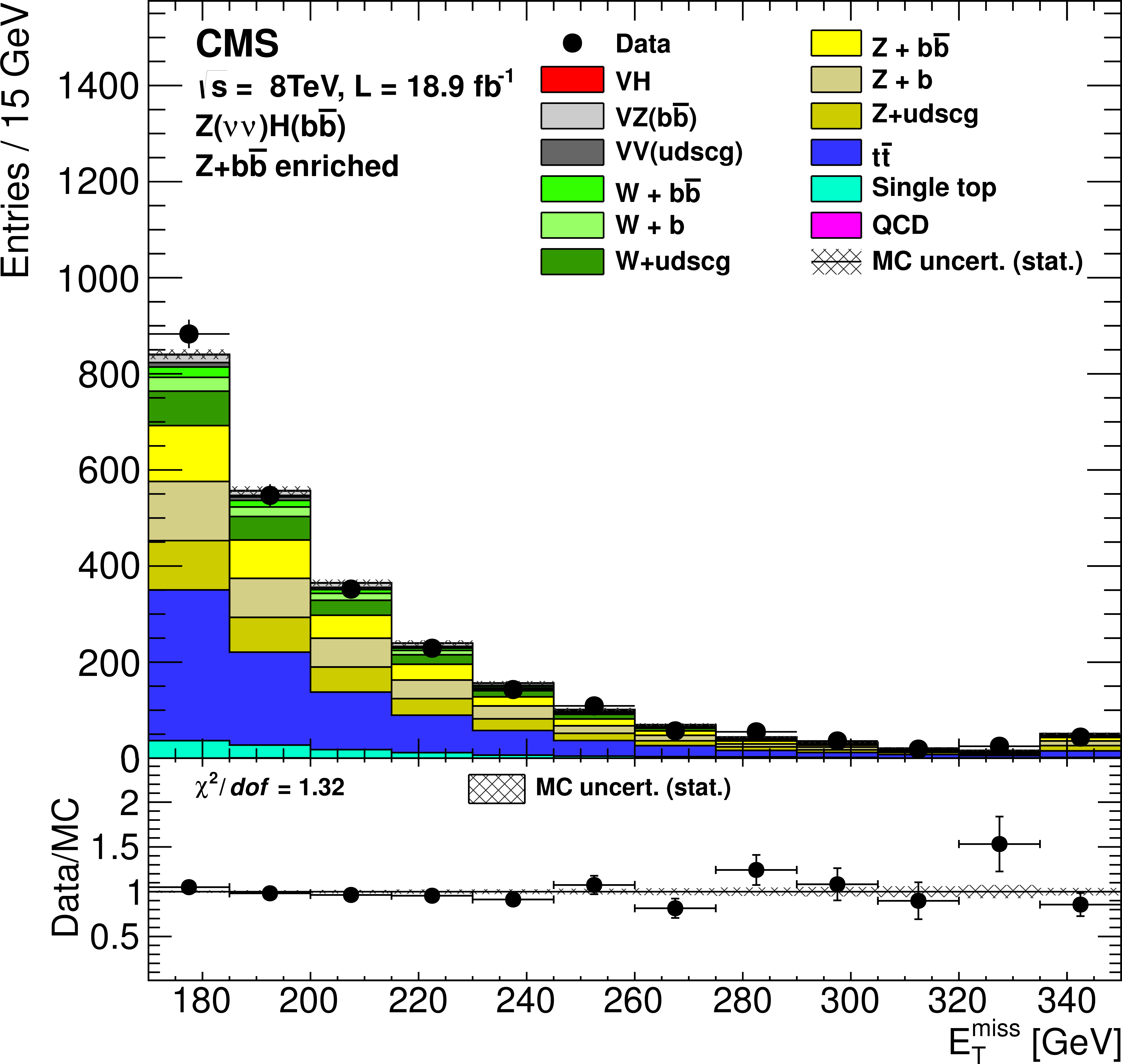
png pdf	Figure 2-a: Examples of distributions for variables in the simulated samples and in data for different control regions and for different channels after applying the data/MC scale factors in Table 7. a: Dijet ${p_{\mathrm {T}}} $ distribution in the $ {\mathrm {Z}}$+jets control region for the ${ {\mathrm {Z}}( {\mathrm {e}} {\mathrm {e}}) {\mathrm {H}} } $ channel. b: ${p_{\mathrm {T}}} $ distribution in the $ {\mathrm {t}\overline {\mathrm {t}}} $ control region for the $ { {\mathrm {W}}( {{\mu }} {\nu }) {\mathrm {H}} } $ channel. c: CSV$_{\text {min}}$ distribution for the $ {\mathrm {W}}$+HF high-boost control region for the ${ {\mathrm {Z}}( {\nu } {\nu }) {\mathrm {H}} } $ channel. d: ${E_{\mathrm {T}}^{\text {miss}}}$ distribution for the ${\mathrm {Z}}$+HF high-boost control region for the ${ {\mathrm {Z}}( {\nu } {\nu }) {\mathrm {H}} } $ channel. The bottom inset in each figure shows the ratio of the number of events observed in data to that of the Monte Carlo prediction for signal and backgrounds.
png pdf	Figure 2-b: Examples of distributions for variables in the simulated samples and in data for different control regions and for different channels after applying the data/MC scale factors in Table 7. a: Dijet ${p_{\mathrm {T}}} $ distribution in the $ {\mathrm {Z}}$+jets control region for the ${ {\mathrm {Z}}( {\mathrm {e}} {\mathrm {e}}) {\mathrm {H}} } $ channel. b: ${p_{\mathrm {T}}} $ distribution in the $ {\mathrm {t}\overline {\mathrm {t}}} $ control region for the $ { {\mathrm {W}}( {{\mu }} {\nu }) {\mathrm {H}} } $ channel. c: CSV$_{\text {min}}$ distribution for the $ {\mathrm {W}}$+HF high-boost control region for the ${ {\mathrm {Z}}( {\nu } {\nu }) {\mathrm {H}} } $ channel. d: ${E_{\mathrm {T}}^{\text {miss}}}$ distribution for the ${\mathrm {Z}}$+HF high-boost control region for the ${ {\mathrm {Z}}( {\nu } {\nu }) {\mathrm {H}} } $ channel. The bottom inset in each figure shows the ratio of the number of events observed in data to that of the Monte Carlo prediction for signal and backgrounds.
png pdf	Figure 2-c: Examples of distributions for variables in the simulated samples and in data for different control regions and for different channels after applying the data/MC scale factors in Table 7. a: Dijet ${p_{\mathrm {T}}} $ distribution in the $ {\mathrm {Z}}$+jets control region for the ${ {\mathrm {Z}}( {\mathrm {e}} {\mathrm {e}}) {\mathrm {H}} } $ channel. b: ${p_{\mathrm {T}}} $ distribution in the $ {\mathrm {t}\overline {\mathrm {t}}} $ control region for the $ { {\mathrm {W}}( {{\mu }} {\nu }) {\mathrm {H}} } $ channel. c: CSV$_{\text {min}}$ distribution for the $ {\mathrm {W}}$+HF high-boost control region for the ${ {\mathrm {Z}}( {\nu } {\nu }) {\mathrm {H}} } $ channel. d: ${E_{\mathrm {T}}^{\text {miss}}}$ distribution for the ${\mathrm {Z}}$+HF high-boost control region for the ${ {\mathrm {Z}}( {\nu } {\nu }) {\mathrm {H}} } $ channel. The bottom inset in each figure shows the ratio of the number of events observed in data to that of the Monte Carlo prediction for signal and backgrounds.
png pdf	Figure 2-d: Examples of distributions for variables in the simulated samples and in data for different control regions and for different channels after applying the data/MC scale factors in Table 7. a: Dijet ${p_{\mathrm {T}}} $ distribution in the $ {\mathrm {Z}}$+jets control region for the ${ {\mathrm {Z}}( {\mathrm {e}} {\mathrm {e}}) {\mathrm {H}} } $ channel. b: ${p_{\mathrm {T}}} $ distribution in the $ {\mathrm {t}\overline {\mathrm {t}}} $ control region for the $ { {\mathrm {W}}( {{\mu }} {\nu }) {\mathrm {H}} } $ channel. c: CSV$_{\text {min}}$ distribution for the $ {\mathrm {W}}$+HF high-boost control region for the ${ {\mathrm {Z}}( {\nu } {\nu }) {\mathrm {H}} } $ channel. d: ${E_{\mathrm {T}}^{\text {miss}}}$ distribution for the ${\mathrm {Z}}$+HF high-boost control region for the ${ {\mathrm {Z}}( {\nu } {\nu }) {\mathrm {H}} } $ channel. The bottom inset in each figure shows the ratio of the number of events observed in data to that of the Monte Carlo prediction for signal and backgrounds.
png pdf	Figure 3-a: Examples of distributions of the event BDT discriminant output in the simulated samples and in data for different control regions and for different channels after applying the data/MC scale factors in Table 7. a: ${\mathrm {W}}$+jets control region for the ${ {\mathrm {W}}( {\mathrm {e}} {\nu }) {\mathrm {H}} } $ channel. b: $ {\mathrm {t}\overline {\mathrm {t}}} $ control region for the ${ {\mathrm {Z}}( {{\mu }} {{\mu }}) {\mathrm {H}} } $ channel. c: ${\mathrm {W}}$+HF high-boost control region for the ${ {\mathrm {Z}}( {\nu } {\nu }) {\mathrm {H}} } $ channel. d: $ {\mathrm {Z}}$+HF high-boost control region for the $ { {\mathrm {Z}}( {\nu } {\nu }) {\mathrm {H}} } $ channel. The bottom inset in each figure shows the ratio of the number of events observed in data to that of the Monte Carlo prediction for signal and backgrounds.
png pdf	Figure 3-b: Examples of distributions of the event BDT discriminant output in the simulated samples and in data for different control regions and for different channels after applying the data/MC scale factors in Table 7. a: ${\mathrm {W}}$+jets control region for the ${ {\mathrm {W}}( {\mathrm {e}} {\nu }) {\mathrm {H}} } $ channel. b: $ {\mathrm {t}\overline {\mathrm {t}}} $ control region for the ${ {\mathrm {Z}}( {{\mu }} {{\mu }}) {\mathrm {H}} } $ channel. c: ${\mathrm {W}}$+HF high-boost control region for the ${ {\mathrm {Z}}( {\nu } {\nu }) {\mathrm {H}} } $ channel. d: $ {\mathrm {Z}}$+HF high-boost control region for the $ { {\mathrm {Z}}( {\nu } {\nu }) {\mathrm {H}} } $ channel. The bottom inset in each figure shows the ratio of the number of events observed in data to that of the Monte Carlo prediction for signal and backgrounds.
png pdf	Figure 3-c: Examples of distributions of the event BDT discriminant output in the simulated samples and in data for different control regions and for different channels after applying the data/MC scale factors in Table 7. a: ${\mathrm {W}}$+jets control region for the ${ {\mathrm {W}}( {\mathrm {e}} {\nu }) {\mathrm {H}} } $ channel. b: $ {\mathrm {t}\overline {\mathrm {t}}} $ control region for the ${ {\mathrm {Z}}( {{\mu }} {{\mu }}) {\mathrm {H}} } $ channel. c: ${\mathrm {W}}$+HF high-boost control region for the ${ {\mathrm {Z}}( {\nu } {\nu }) {\mathrm {H}} } $ channel. d: $ {\mathrm {Z}}$+HF high-boost control region for the $ { {\mathrm {Z}}( {\nu } {\nu }) {\mathrm {H}} } $ channel. The bottom inset in each figure shows the ratio of the number of events observed in data to that of the Monte Carlo prediction for signal and backgrounds.
png pdf	Figure 3-d: Examples of distributions of the event BDT discriminant output in the simulated samples and in data for different control regions and for different channels after applying the data/MC scale factors in Table 7. a: ${\mathrm {W}}$+jets control region for the ${ {\mathrm {W}}( {\mathrm {e}} {\nu }) {\mathrm {H}} } $ channel. b: $ {\mathrm {t}\overline {\mathrm {t}}} $ control region for the ${ {\mathrm {Z}}( {{\mu }} {{\mu }}) {\mathrm {H}} } $ channel. c: ${\mathrm {W}}$+HF high-boost control region for the ${ {\mathrm {Z}}( {\nu } {\nu }) {\mathrm {H}} } $ channel. d: $ {\mathrm {Z}}$+HF high-boost control region for the $ { {\mathrm {Z}}( {\nu } {\nu }) {\mathrm {H}} } $ channel. The bottom inset in each figure shows the ratio of the number of events observed in data to that of the Monte Carlo prediction for signal and backgrounds.
png pdf	Figure 4-a: Post-fit BDT output distributions for ${ {\mathrm {Z}}( {\nu } {\nu }) {\mathrm {H}} } $ in the high-boost region for 8 TeV data (points with error bars), all backgrounds, and signal, after all selection criteria have been applied. The event BDT discriminant values for events in the four different subsets are rescaled and offset to assemble a single BDT output variable. This leads to the four equally-sized partitions shown in the left panel. The partitions correspond, starting from the left, to the event subsets enriched in ${\mathrm {t}\overline {\mathrm {t}}} , { {\mathrm {V}} }$+jets, diboson, and $ {{ {\mathrm {V}} } {\mathrm {H}} }$ production. The Fig.4-b shows the right-most, ${{ {\mathrm {V}} } {\mathrm {H}} } $-enriched, partition in more detail. The bottom inset in each figure shows the ratio of the number of events observed in data to that of the Monte Carlo prediction for signal and backgrounds.
png pdf	Figure 4-b: Post-fit BDT output distributions for ${ {\mathrm {Z}}( {\nu } {\nu }) {\mathrm {H}} } $ in the high-boost region for 8 TeV data (points with error bars), all backgrounds, and signal, after all selection criteria have been applied. The event BDT discriminant values for events in the four different subsets are rescaled and offset to assemble a single BDT output variable. This leads to the four equally-sized partitions shown in the left panel. The partitions correspond, starting from the left, to the event subsets enriched in ${\mathrm {t}\overline {\mathrm {t}}} , { {\mathrm {V}} }$+jets, diboson, and $ {{ {\mathrm {V}} } {\mathrm {H}} }$ production. The Fig.4-b shows the right-most, ${{ {\mathrm {V}} } {\mathrm {H}} } $-enriched, partition in more detail. The bottom inset in each figure shows the ratio of the number of events observed in data to that of the Monte Carlo prediction for signal and backgrounds.
png pdf	Figure 5: Combination of all channels into a single distribution. Events are sorted in bins of similar expected signal-to-background ratio, as given by the value of the output of their corresponding BDT discriminant (trained with a Higgs boson mass hypothesis of 125 GeV). The two bottom insets show the ratio of the data to the background-only prediction (above) and to the predicted sum of background and SM Higgs boson signal with a mass of 125 GeV (below).
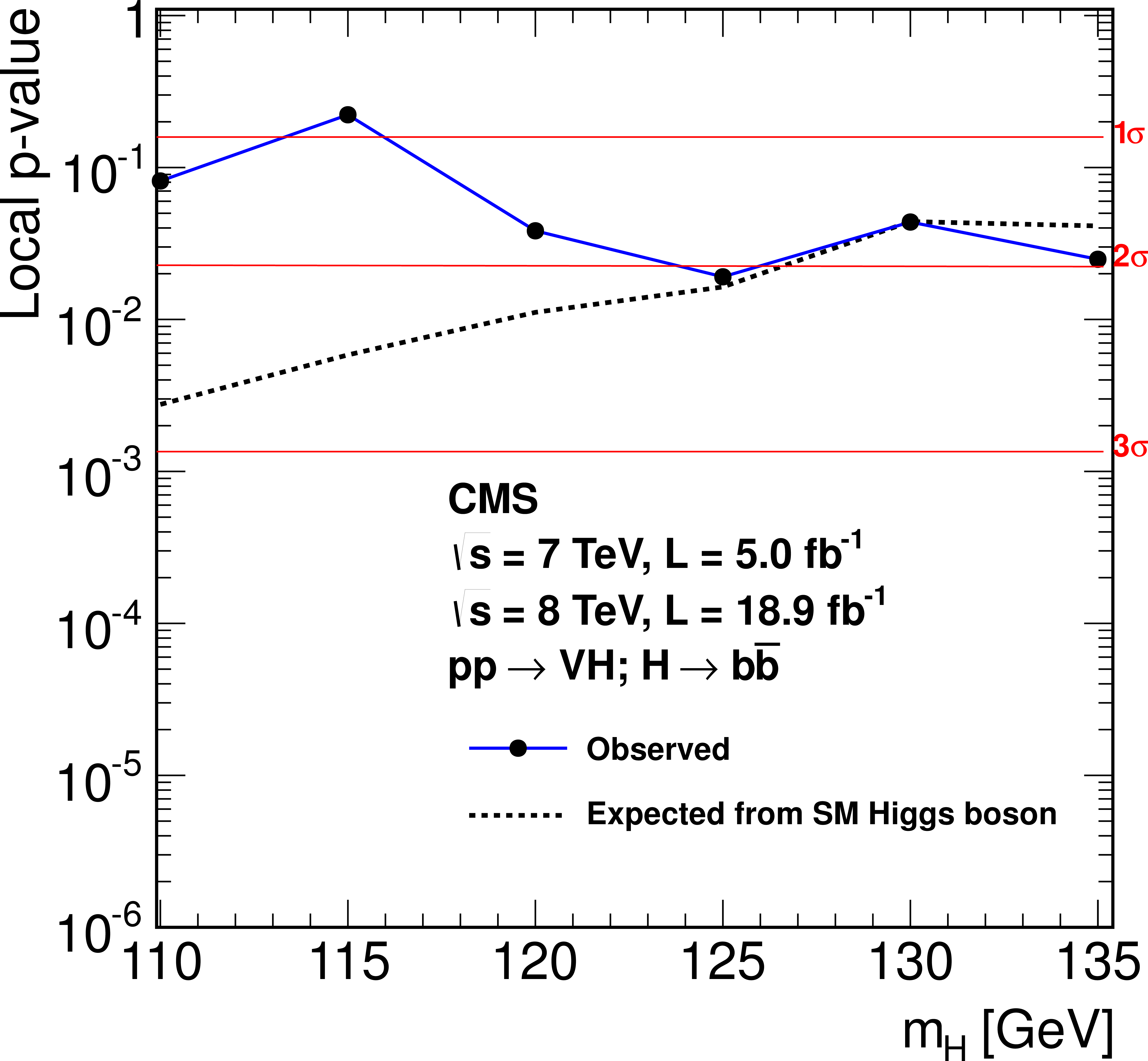
png pdf	Figure 6-a: a: The expected and observed 95% CL upper limits on the product of the $ {{ {\mathrm {V}} } {\mathrm {H}} } $ production cross section times the ${ {\mathrm {H}} \to { {\mathrm {b}} {\overline {\mathrm {b}}}} } $ branching fraction, with respect to the expectations for the standard model Higgs boson. The limits are obtained combining the results of the searches using the 2011 (7 TeV) and 2012 (8 TeV) data. The red dashed line represents the expected limit obtained from the sum of expected backgrounds and the SM Higgs boson signal with a mass of 125 GeV. b: local p-values and corresponding significance (measured in standard deviations) for the background-only hypothesis to account for the observed excess of events in the data.
png pdf	Figure 6-b: a: The expected and observed 95% CL upper limits on the product of the $ {{ {\mathrm {V}} } {\mathrm {H}} } $ production cross section times the ${ {\mathrm {H}} \to { {\mathrm {b}} {\overline {\mathrm {b}}}} } $ branching fraction, with respect to the expectations for the standard model Higgs boson. The limits are obtained combining the results of the searches using the 2011 (7 TeV) and 2012 (8 TeV) data. The red dashed line represents the expected limit obtained from the sum of expected backgrounds and the SM Higgs boson signal with a mass of 125 GeV. b: local p-values and corresponding significance (measured in standard deviations) for the background-only hypothesis to account for the observed excess of events in the data.
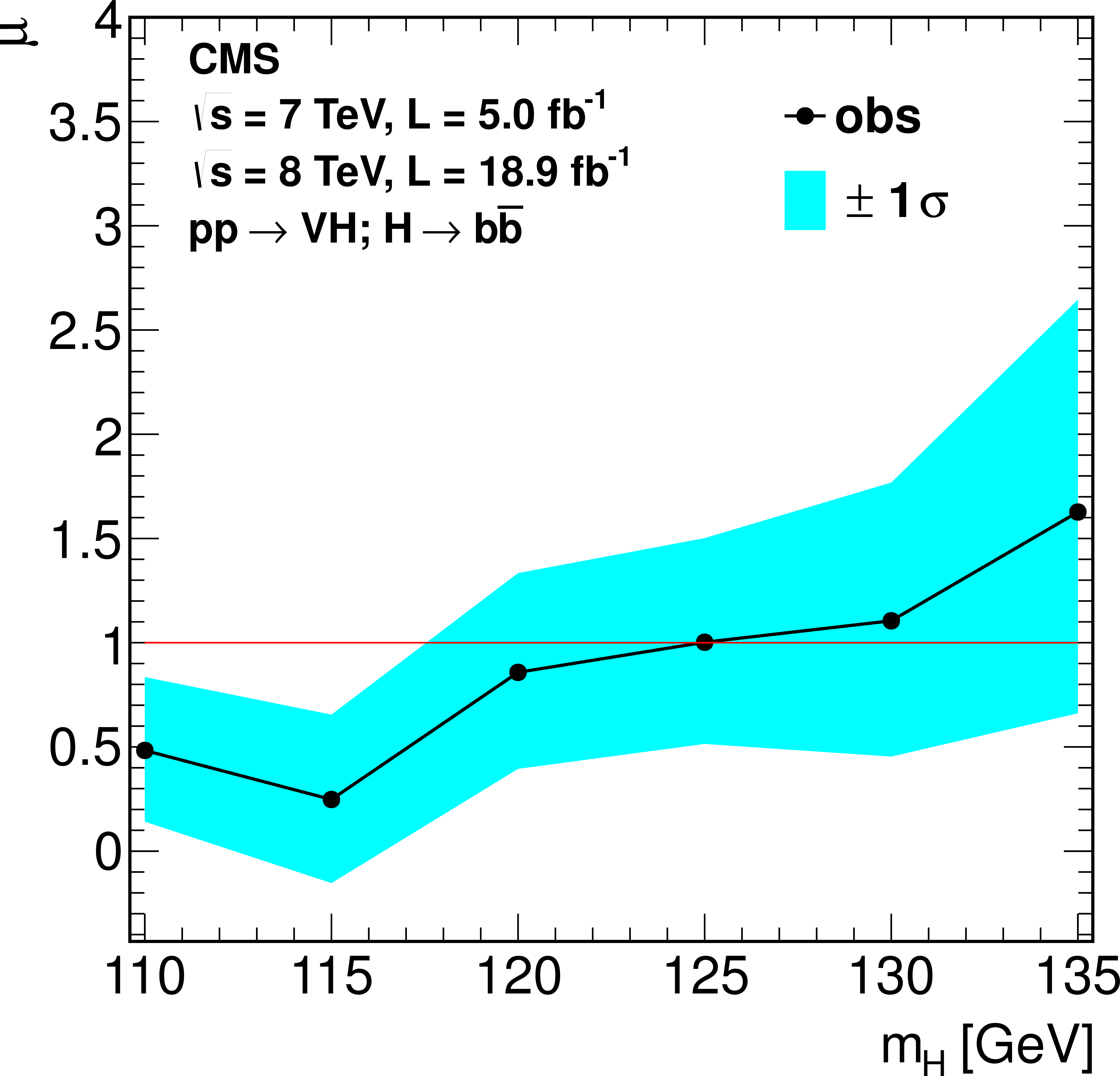
png pdf	Figure 7-a: a: The best-fit value of the production cross section for a 125 GeV Higgs boson relative to the standard model cross section, i.e., signal strength $\mu $, for partial combinations of channels and for all channels combined (band). b: The best-fit values and the 68% and 95% CL contour regions for the $\mu _{ { {\mathrm {Z}} {\mathrm {H}} } }$, $\mu _{ { {\mathrm {W}} {\mathrm {H}} } }$ signal strength parameters for a 125 GeV Higgs boson.
png pdf	Figure 7-b: a: The best-fit value of the production cross section for a 125 GeV Higgs boson relative to the standard model cross section, i.e., signal strength $\mu $, for partial combinations of channels and for all channels combined (band). b: The best-fit values and the 68% and 95% CL contour regions for the $\mu _{ { {\mathrm {Z}} {\mathrm {H}} } }$, $\mu _{ { {\mathrm {W}} {\mathrm {H}} } }$ signal strength parameters for a 125 GeV Higgs boson.
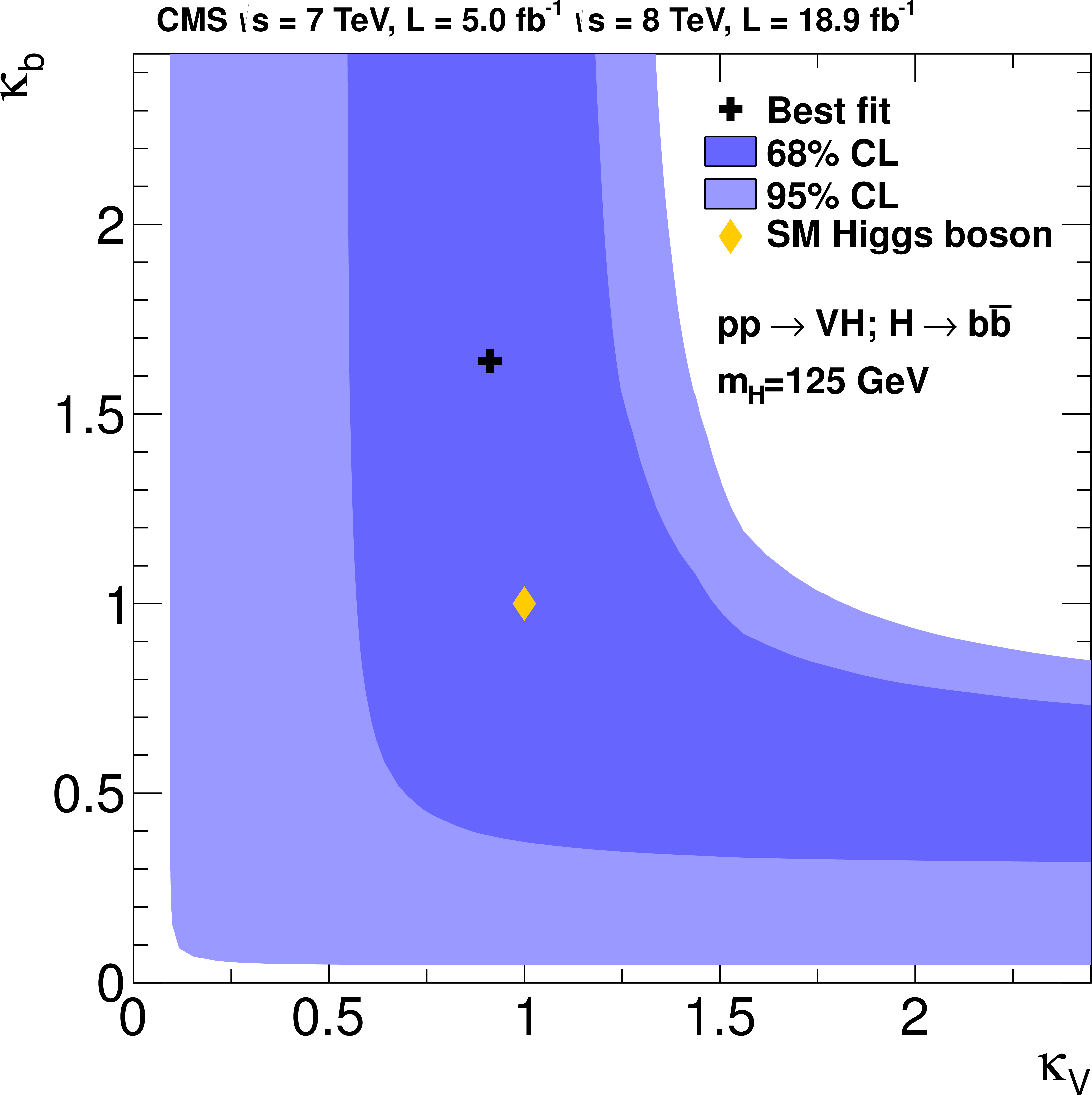
png pdf	Figure 8-a: a: Signal strength for all channels combined as a function of the value assumed for the Higgs boson mass. Right: The best-fit values and the 68% and 95% CL contour regions for the $\kappa _ {\mathrm {V}} $ and $\kappa _ {\mathrm {b}}$ parameters. The cross indicates the best-fit values and the yellow diamond shows the SM point $(\kappa _ {\mathrm {V}} , \kappa _ {\mathrm {b}}) = (1, 1)$. The likelihood fit is performed in the positive quadrant only.
png pdf	Figure 8-b: a: Signal strength for all channels combined as a function of the value assumed for the Higgs boson mass. Right: The best-fit values and the 68% and 95% CL contour regions for the $\kappa _ {\mathrm {V}} $ and $\kappa _ {\mathrm {b}}$ parameters. The cross indicates the best-fit values and the yellow diamond shows the SM point $(\kappa _ {\mathrm {V}} , \kappa _ {\mathrm {b}}) = (1, 1)$. The likelihood fit is performed in the positive quadrant only.
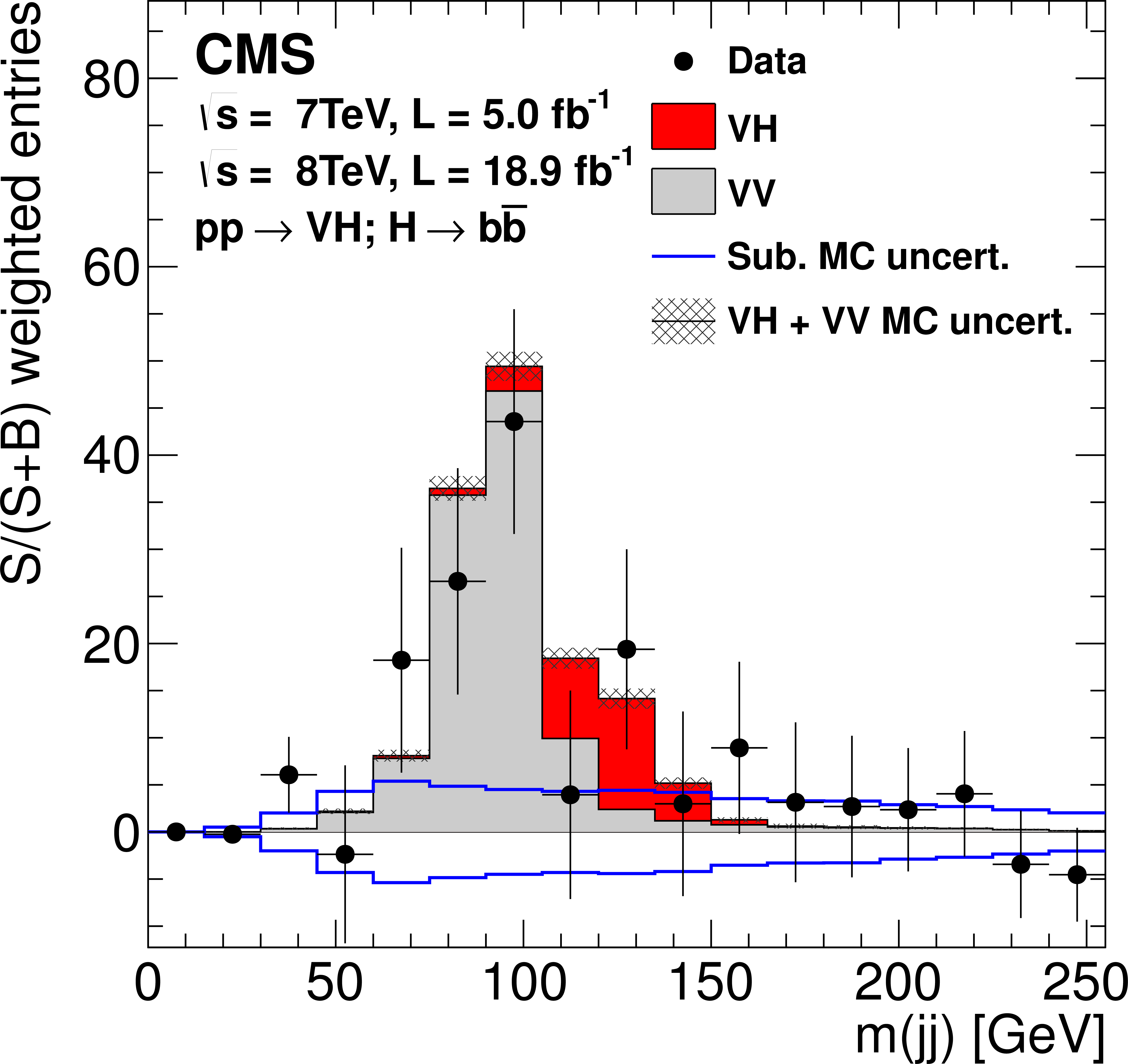
png pdf	Figure 9-a: Dijet mass cross-check analysis. a: weighted dijet invariant mass distribution, combined for all channels. For each channel, the relative dijet mass distribution weight for each boost region is obtained from the ratio of the expected number of signal events to the sum of expected signal and background events in a window of ${m(\mathrm {jj})}$ values between 105 and 150 GeV. The expected signal used corresponds to the production of the SM Higgs boson with a mass of 125 GeV. The weight for the highest-boost region is set to 1.0 and all other weights are adjusted proportionally. The solid histograms for the backgrounds and the signal are summed cumulatively. The line histogram for signal and for ${ {\mathrm {V}} }{ {\mathrm {V}} }$ backgrounds are also shown superimposed. The data is represented by points. The bottom inset shows the ratio of the number of events observed in data to that of the Monte Carlo prediction for signal and backgrounds. b: same distribution with all backgrounds, except dibosons, subtracted.
png pdf	Figure 9-b: Dijet mass cross-check analysis. a: weighted dijet invariant mass distribution, combined for all channels. For each channel, the relative dijet mass distribution weight for each boost region is obtained from the ratio of the expected number of signal events to the sum of expected signal and background events in a window of ${m(\mathrm {jj})}$ values between 105 and 150 GeV. The expected signal used corresponds to the production of the SM Higgs boson with a mass of 125 GeV. The weight for the highest-boost region is set to 1.0 and all other weights are adjusted proportionally. The solid histograms for the backgrounds and the signal are summed cumulatively. The line histogram for signal and for ${ {\mathrm {V}} }{ {\mathrm {V}} }$ backgrounds are also shown superimposed. The data is represented by points. The bottom inset shows the ratio of the number of events observed in data to that of the Monte Carlo prediction for signal and backgrounds. b: same distribution with all backgrounds, except dibosons, subtracted.
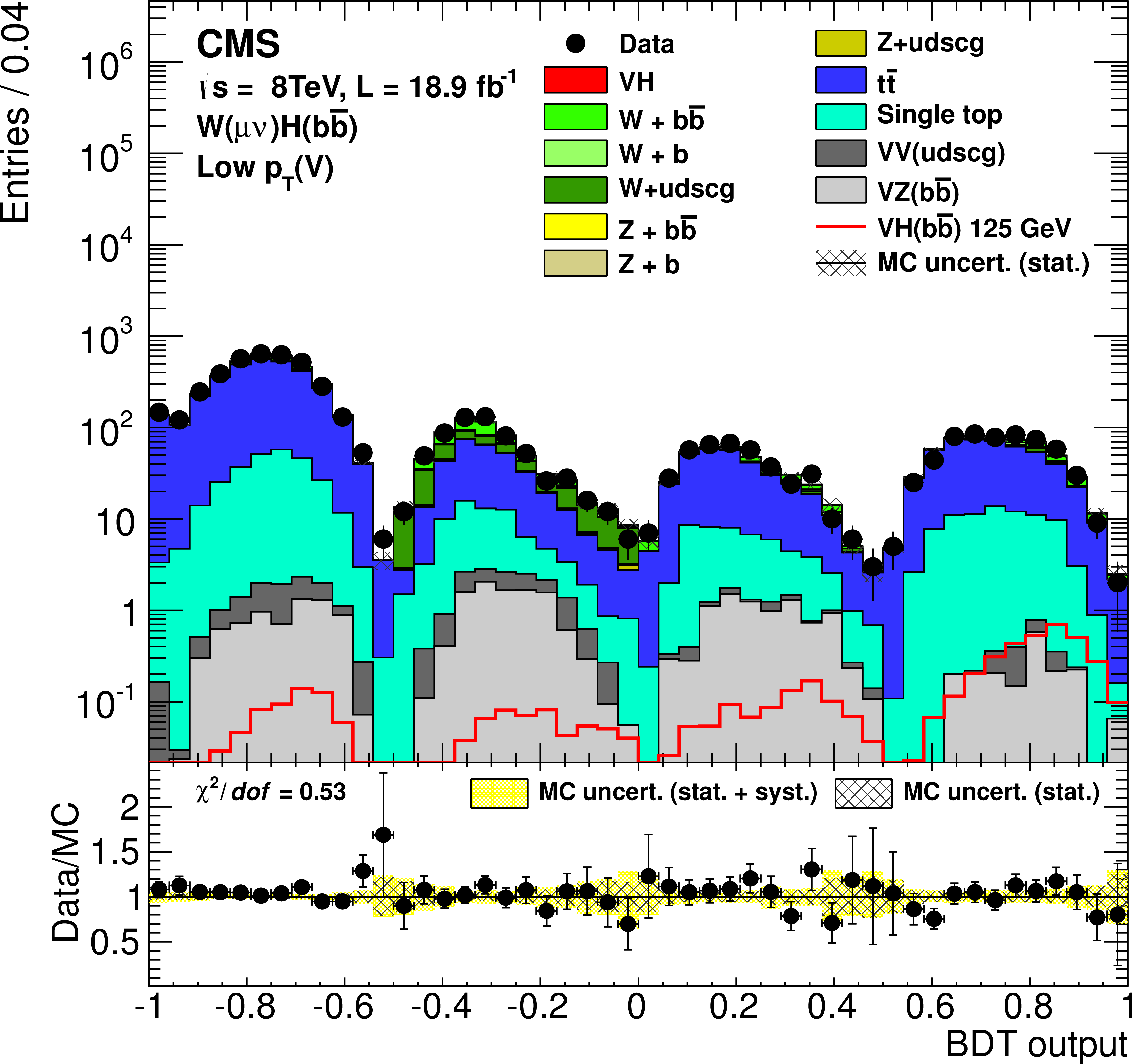
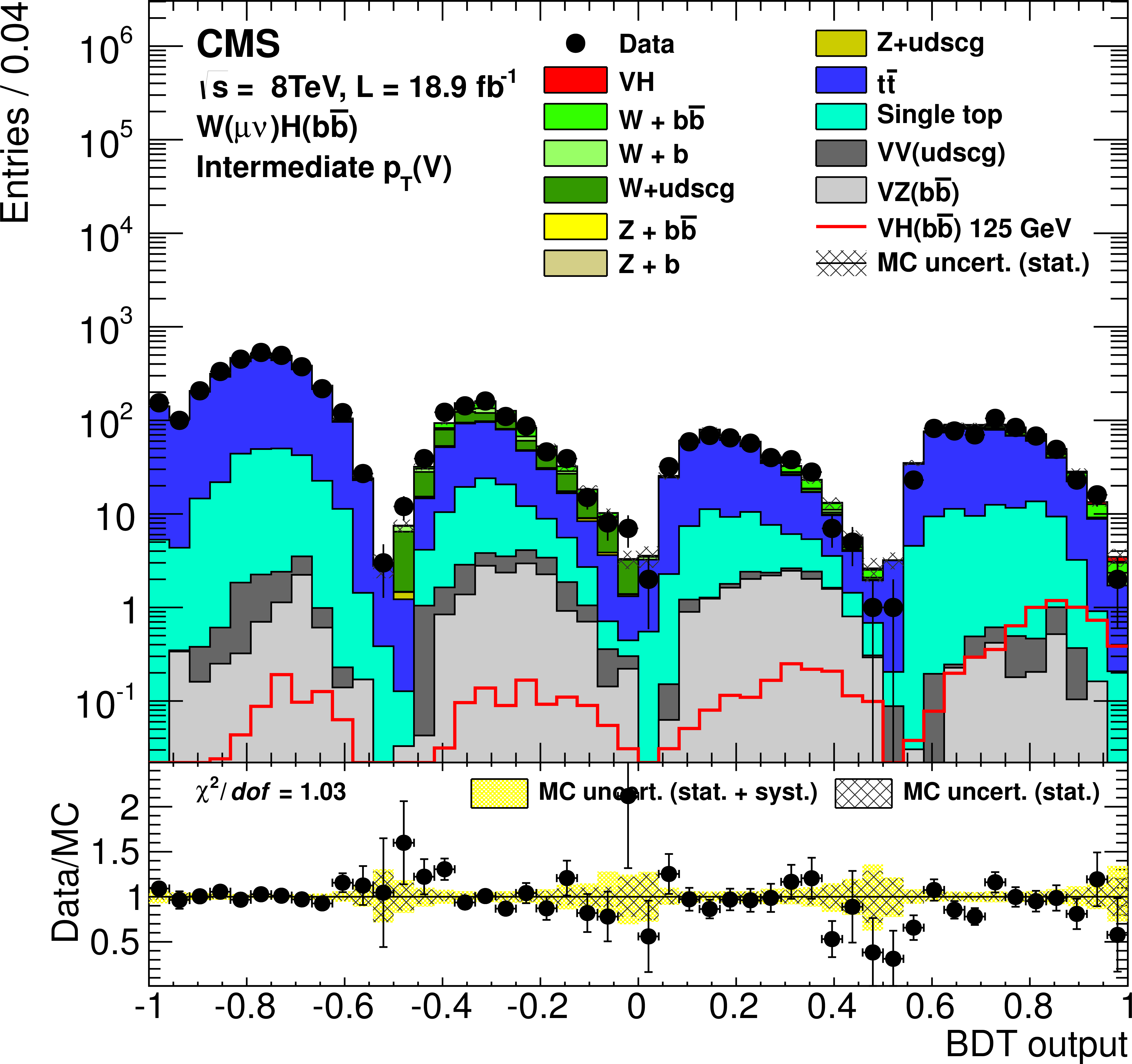
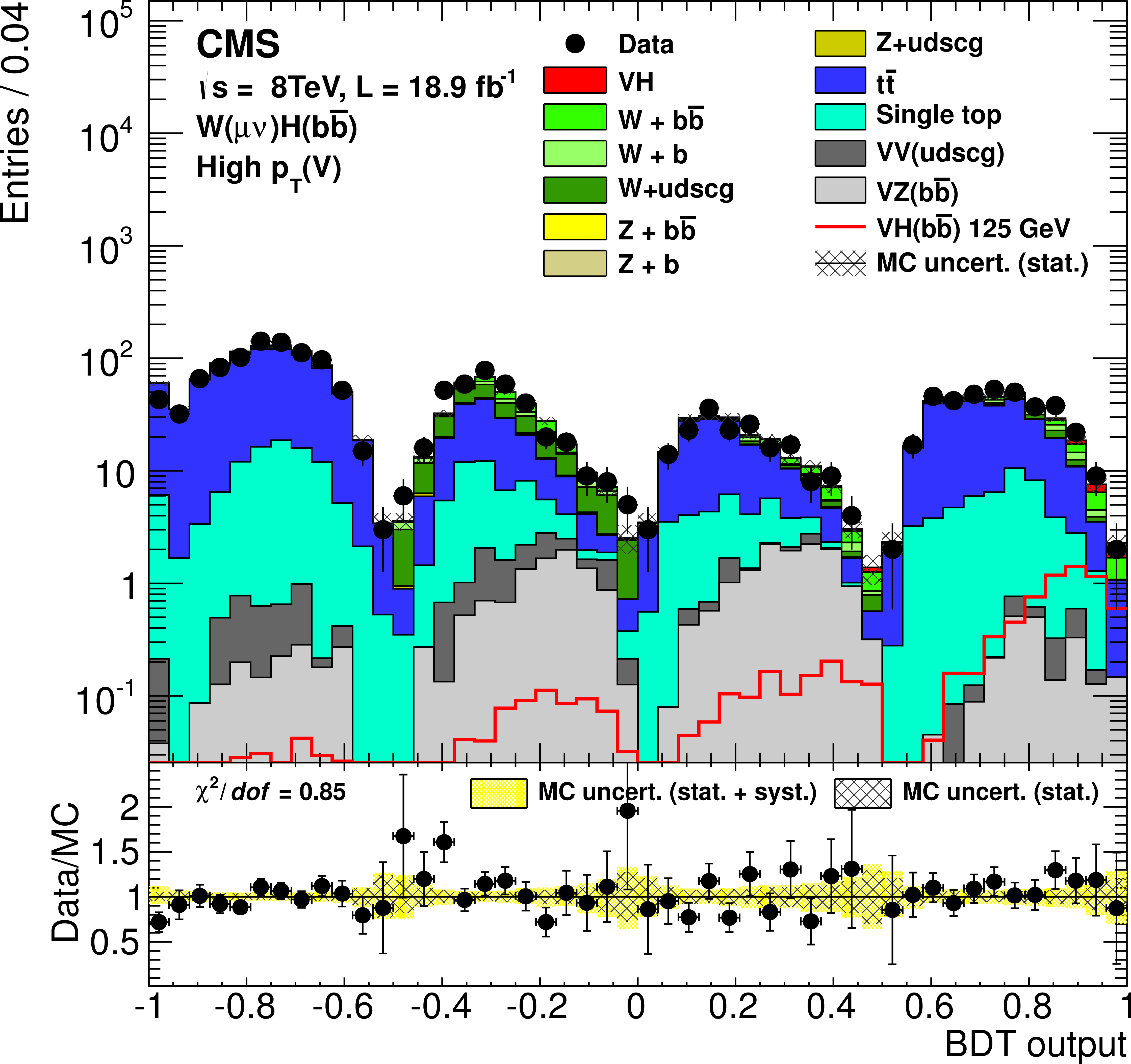
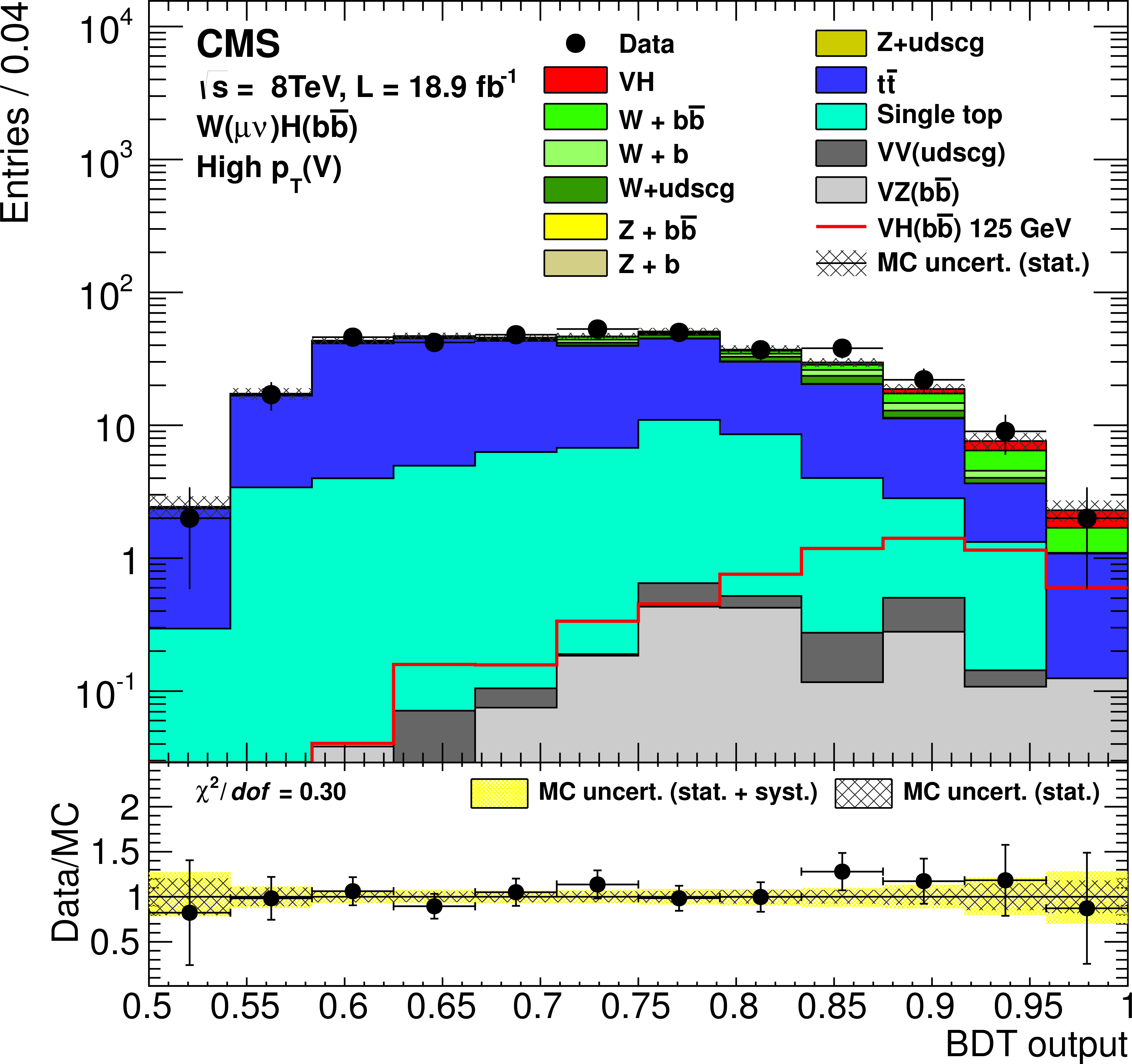
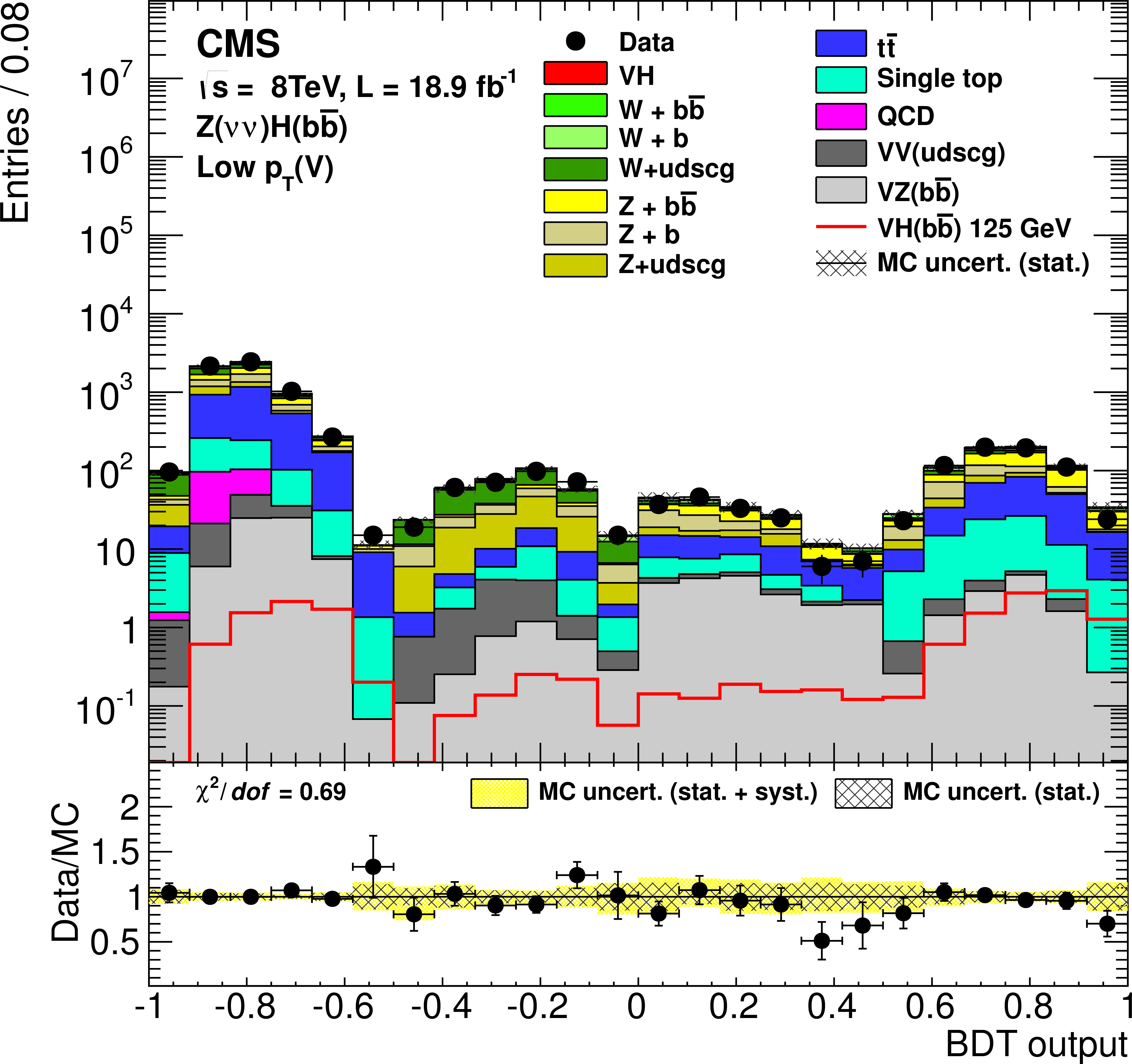
png pdf	Figure 10-a: Post-fit BDT output distributions for ${ {\mathrm {W}}( {{\mu }} {\nu }) {\mathrm {H}} } $ in the low-boost region (a), the intermediate-boost (b), and the high-boost (c, d), for 8 TeV data (points with error bars), all backgrounds, and signal, after all selection criteria have been applied. d: the $ {{ {\mathrm {V}} } {\mathrm {H}} }$-enriched partition of the high-boost region is shown in more detail. The bottom inset in each figure shows the ratio of the number of events observed in data to that of the Monte Carlo prediction for signal and backgrounds.
png pdf	Figure 10-b: Post-fit BDT output distributions for ${ {\mathrm {W}}( {{\mu }} {\nu }) {\mathrm {H}} } $ in the low-boost region (a), the intermediate-boost (b), and the high-boost (c, d), for 8 TeV data (points with error bars), all backgrounds, and signal, after all selection criteria have been applied. d: the $ {{ {\mathrm {V}} } {\mathrm {H}} }$-enriched partition of the high-boost region is shown in more detail. The bottom inset in each figure shows the ratio of the number of events observed in data to that of the Monte Carlo prediction for signal and backgrounds.
png pdf	Figure 10-c: Post-fit BDT output distributions for ${ {\mathrm {W}}( {{\mu }} {\nu }) {\mathrm {H}} } $ in the low-boost region (a), the intermediate-boost (b), and the high-boost (c, d), for 8 TeV data (points with error bars), all backgrounds, and signal, after all selection criteria have been applied. d: the $ {{ {\mathrm {V}} } {\mathrm {H}} }$-enriched partition of the high-boost region is shown in more detail. The bottom inset in each figure shows the ratio of the number of events observed in data to that of the Monte Carlo prediction for signal and backgrounds.
png pdf	Figure 10-d: Post-fit BDT output distributions for ${ {\mathrm {W}}( {{\mu }} {\nu }) {\mathrm {H}} } $ in the low-boost region (a), the intermediate-boost (b), and the high-boost (c, d), for 8 TeV data (points with error bars), all backgrounds, and signal, after all selection criteria have been applied. d: the $ {{ {\mathrm {V}} } {\mathrm {H}} }$-enriched partition of the high-boost region is shown in more detail. The bottom inset in each figure shows the ratio of the number of events observed in data to that of the Monte Carlo prediction for signal and backgrounds.
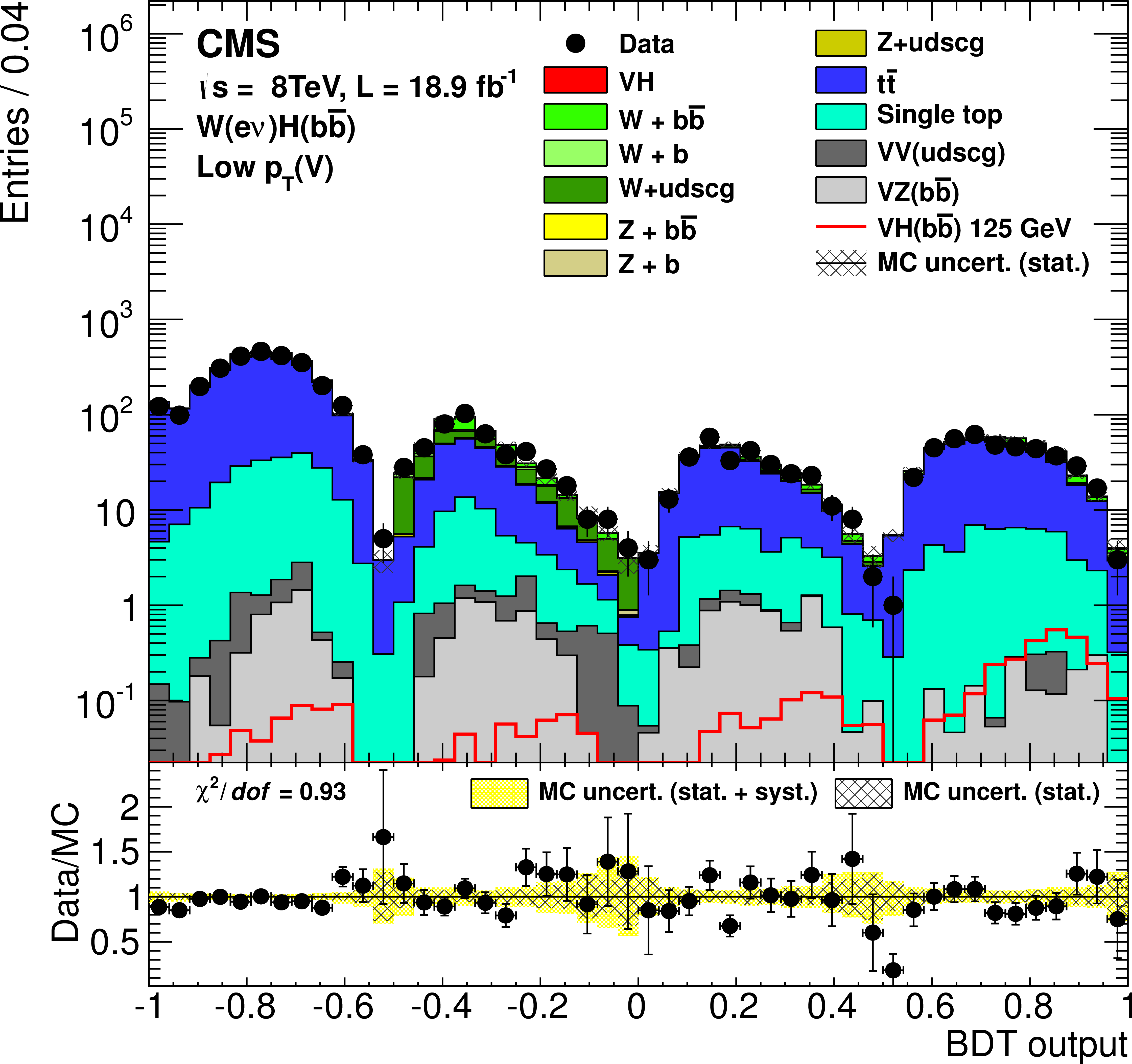
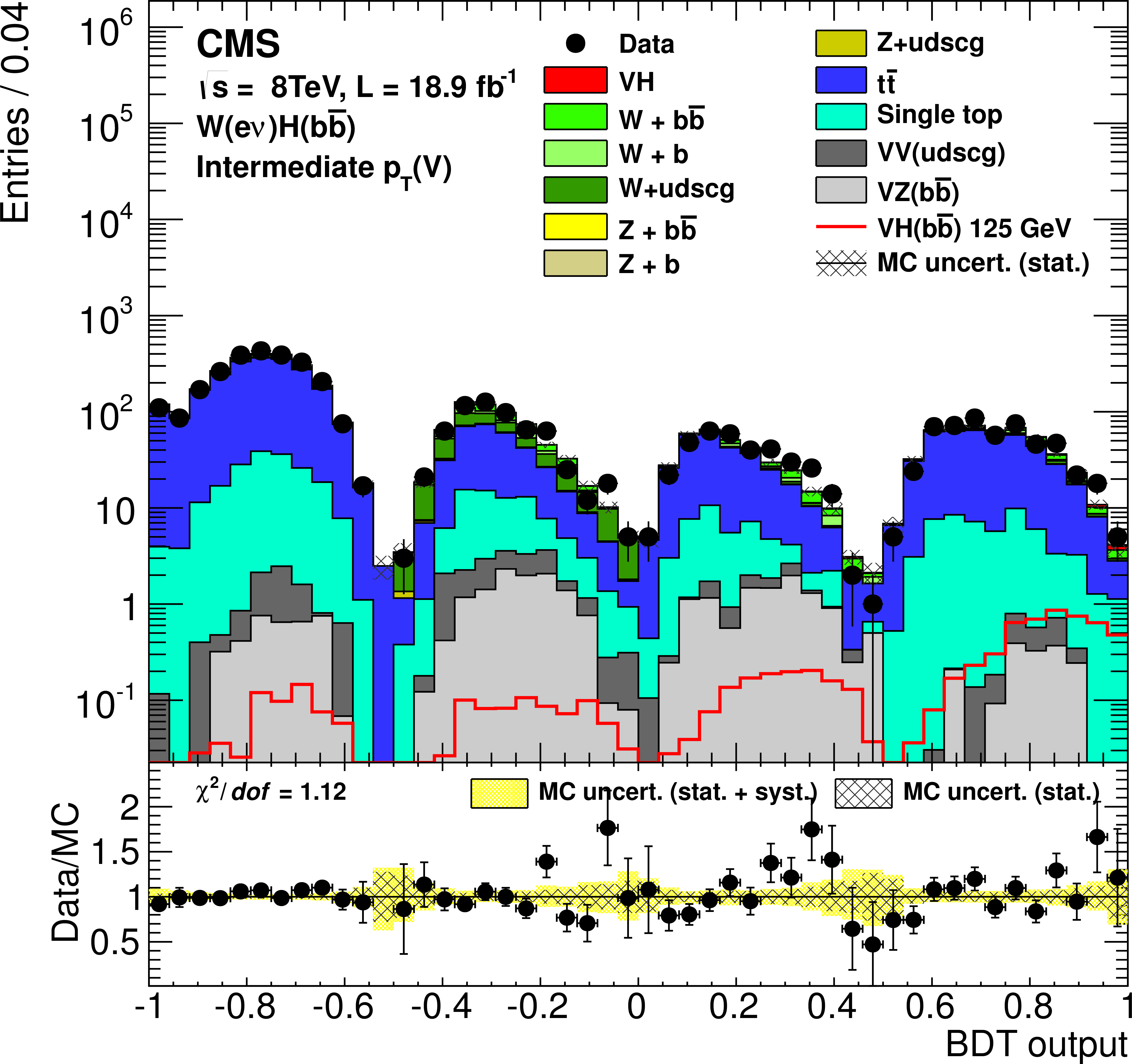
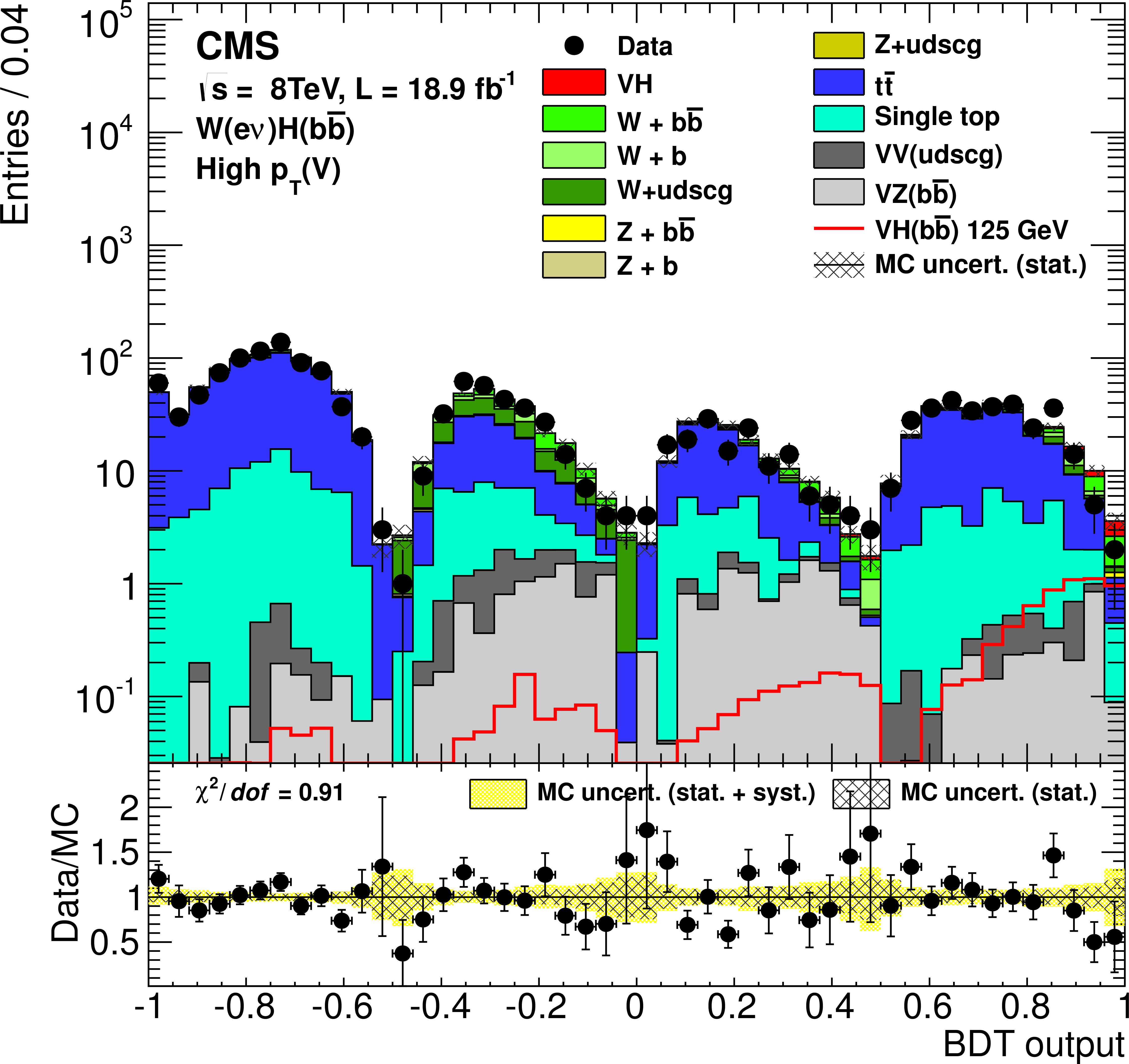
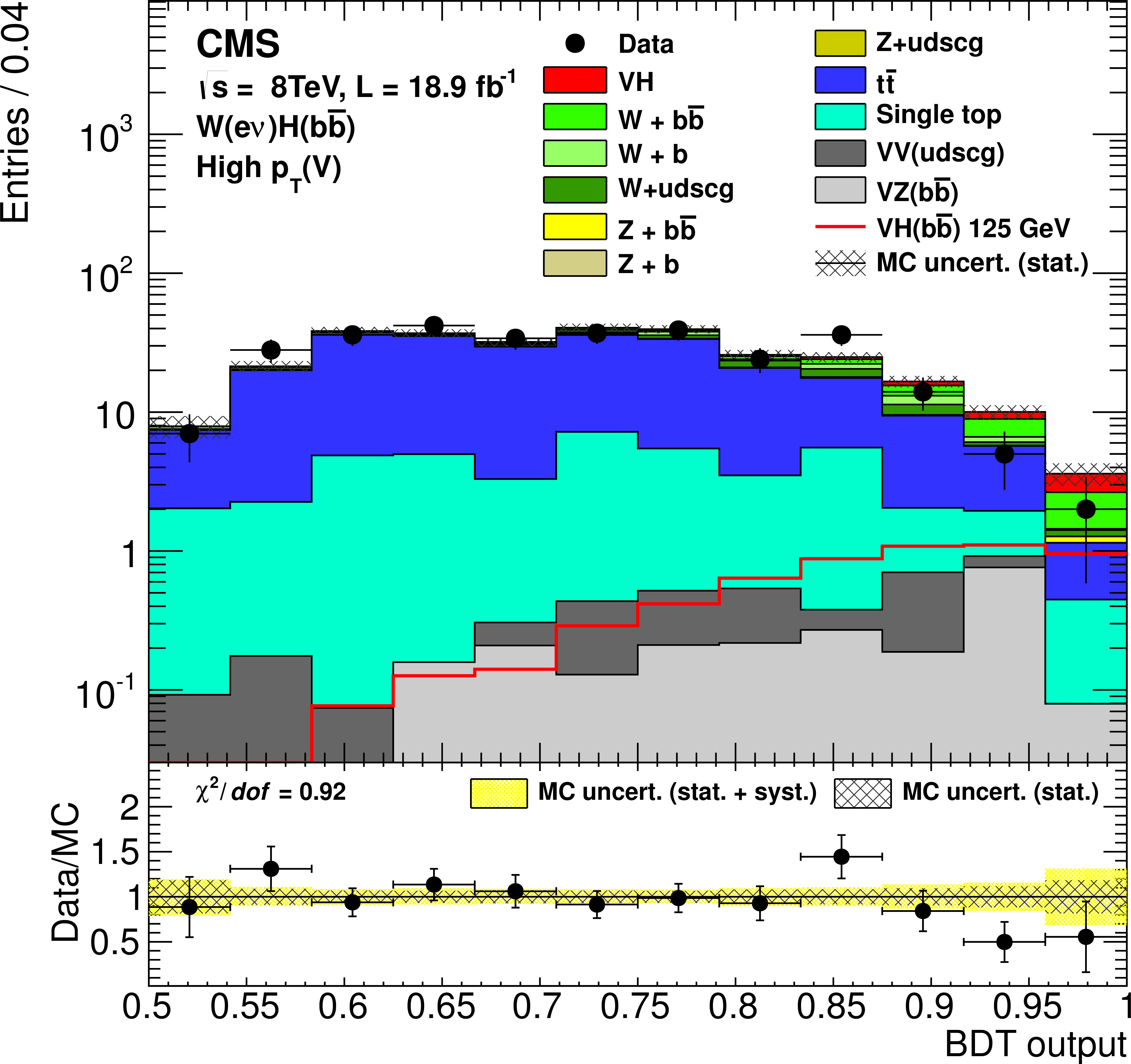
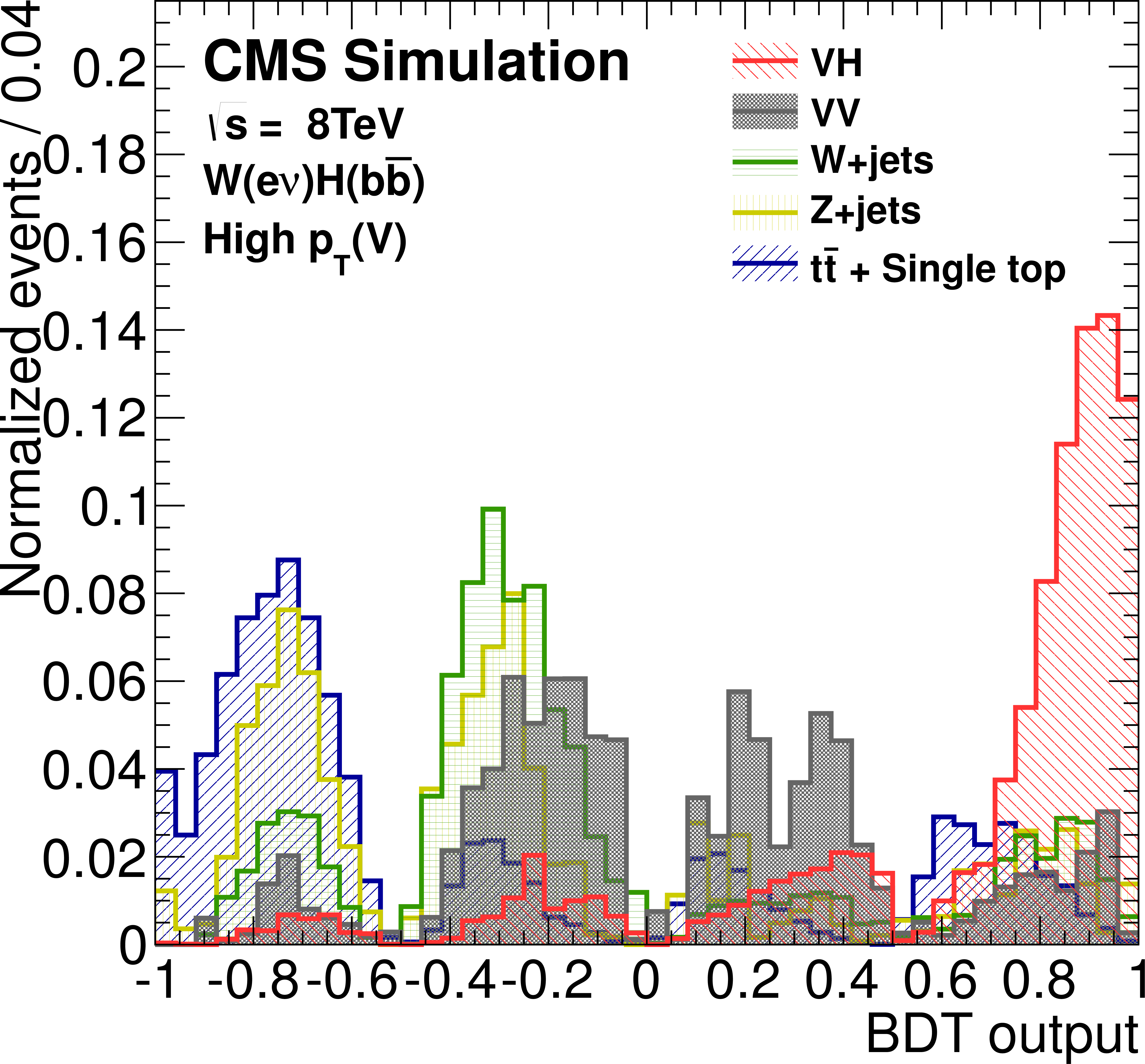
png pdf	Figure 11-a: Post-fit BDT output distributions for ${ {\mathrm {W}}( {\mathrm {e}} {\nu }) {\mathrm {H}} } $ in the low-boost region (a), the intermediate-boost (b), and the high-boost (c, d), for 8 TeV data (points with error bars), all backgrounds, and signal, after all selection criteria have been applied. Bottom right: the ${{ {\mathrm {V}} } {\mathrm {H}} }$-enriched partition of the high-boost region is shown in more detail. The bottom inset in each figure shows the ratio of the number of events observed in data to that of the Monte Carlo prediction for signal and backgrounds.
png pdf	Figure 11-b: Post-fit BDT output distributions for ${ {\mathrm {W}}( {\mathrm {e}} {\nu }) {\mathrm {H}} } $ in the low-boost region (a), the intermediate-boost (b), and the high-boost (c, d), for 8 TeV data (points with error bars), all backgrounds, and signal, after all selection criteria have been applied. Bottom right: the ${{ {\mathrm {V}} } {\mathrm {H}} }$-enriched partition of the high-boost region is shown in more detail. The bottom inset in each figure shows the ratio of the number of events observed in data to that of the Monte Carlo prediction for signal and backgrounds.
png pdf	Figure 11-c: Post-fit BDT output distributions for ${ {\mathrm {W}}( {\mathrm {e}} {\nu }) {\mathrm {H}} } $ in the low-boost region (a), the intermediate-boost (b), and the high-boost (c, d), for 8 TeV data (points with error bars), all backgrounds, and signal, after all selection criteria have been applied. Bottom right: the ${{ {\mathrm {V}} } {\mathrm {H}} }$-enriched partition of the high-boost region is shown in more detail. The bottom inset in each figure shows the ratio of the number of events observed in data to that of the Monte Carlo prediction for signal and backgrounds.
png pdf	Figure 11-d: Post-fit BDT output distributions for ${ {\mathrm {W}}( {\mathrm {e}} {\nu }) {\mathrm {H}} } $ in the low-boost region (a), the intermediate-boost (b), and the high-boost (c, d), for 8 TeV data (points with error bars), all backgrounds, and signal, after all selection criteria have been applied. Bottom right: the ${{ {\mathrm {V}} } {\mathrm {H}} }$-enriched partition of the high-boost region is shown in more detail. The bottom inset in each figure shows the ratio of the number of events observed in data to that of the Monte Carlo prediction for signal and backgrounds.
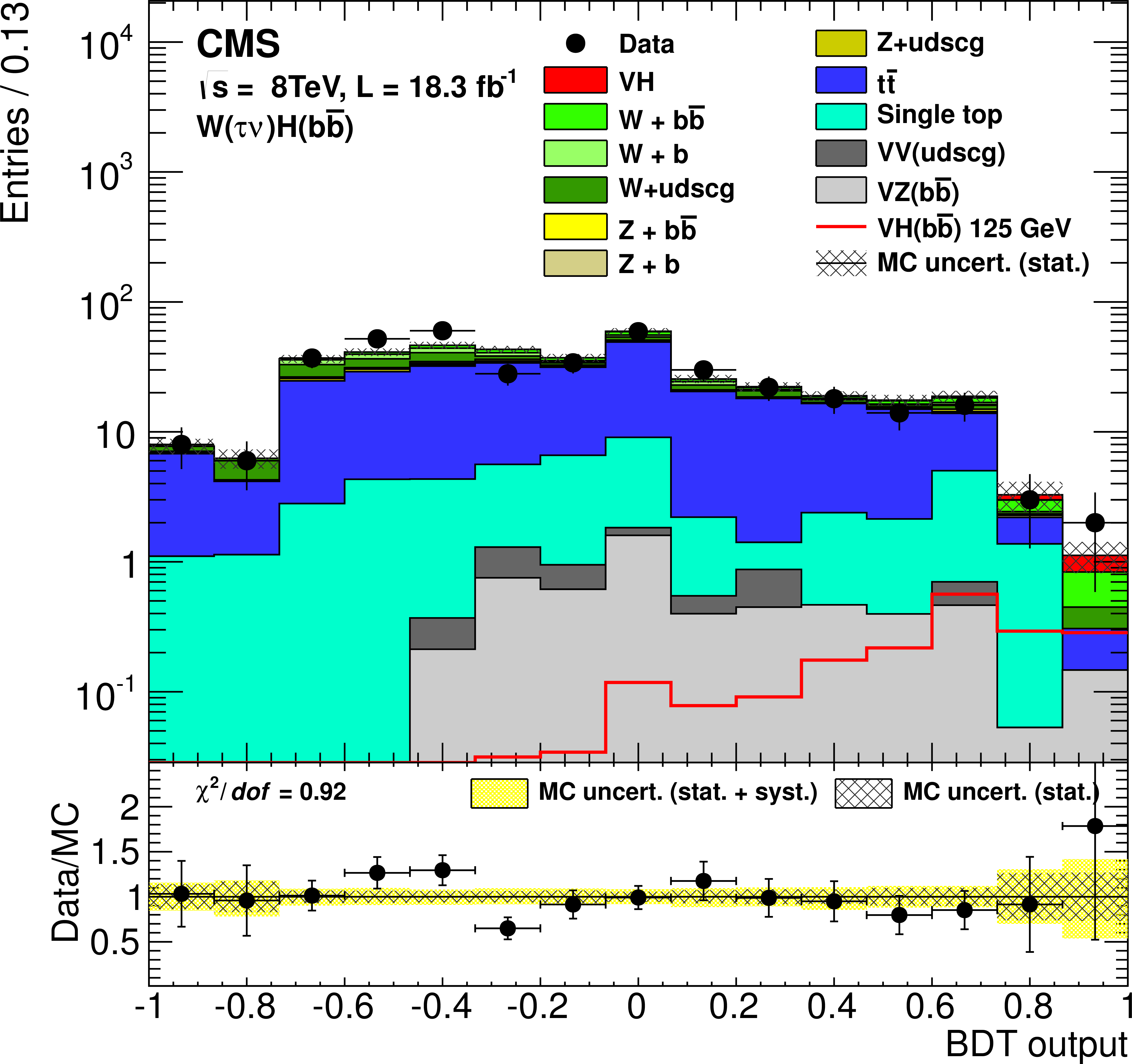
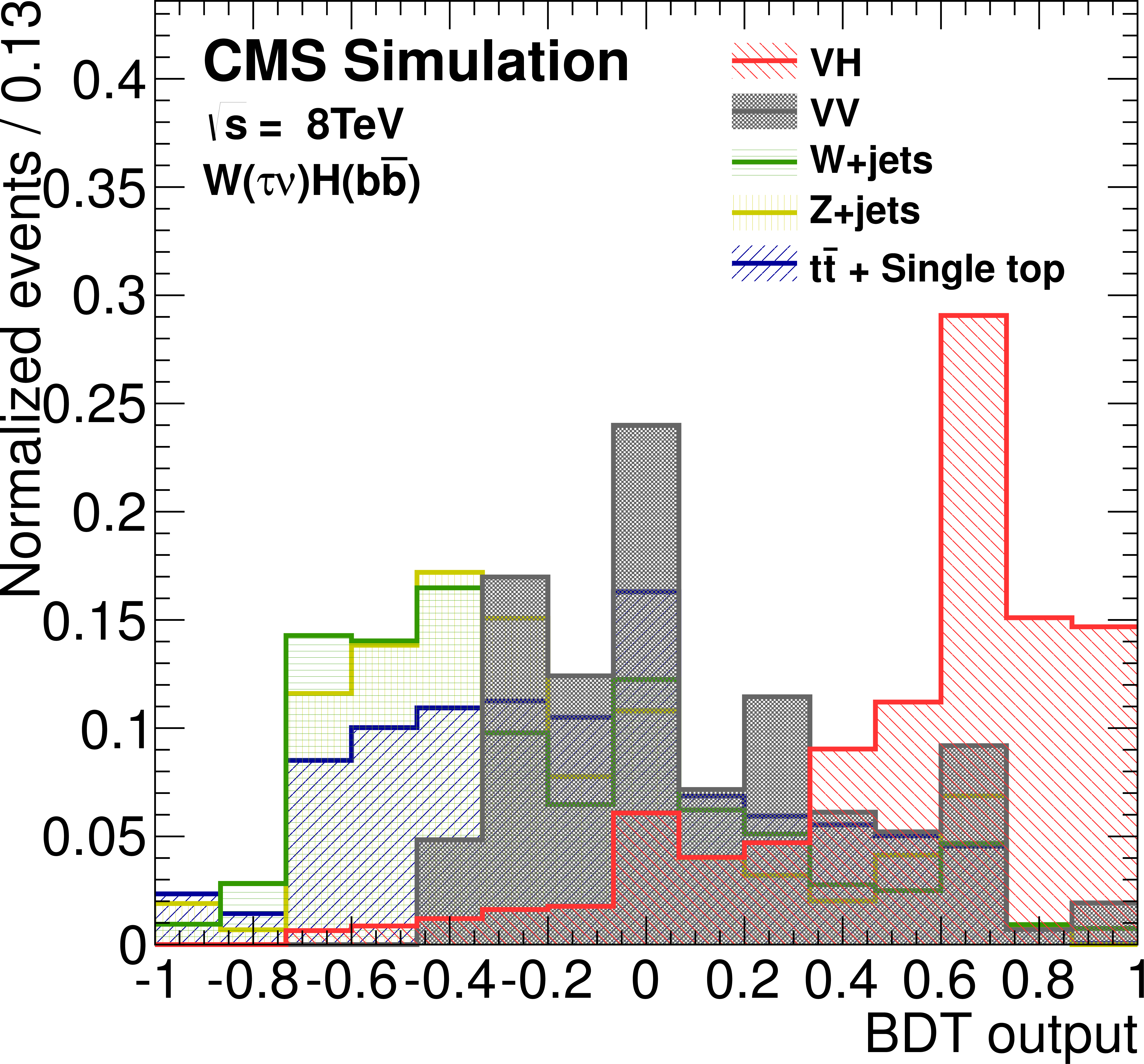
png pdf	Figure 12: Post-fit BDT output distributions for $ { {\mathrm {W}}( {\tau } {\nu }) {\mathrm {H}} } $ for 8 TeV data (points with error bars), all backgrounds, and signal, after all selection criteria have been applied. The bottom inset shows the ratio of the number of events observed in data to that of the Monte Carlo prediction for signal and backgrounds.
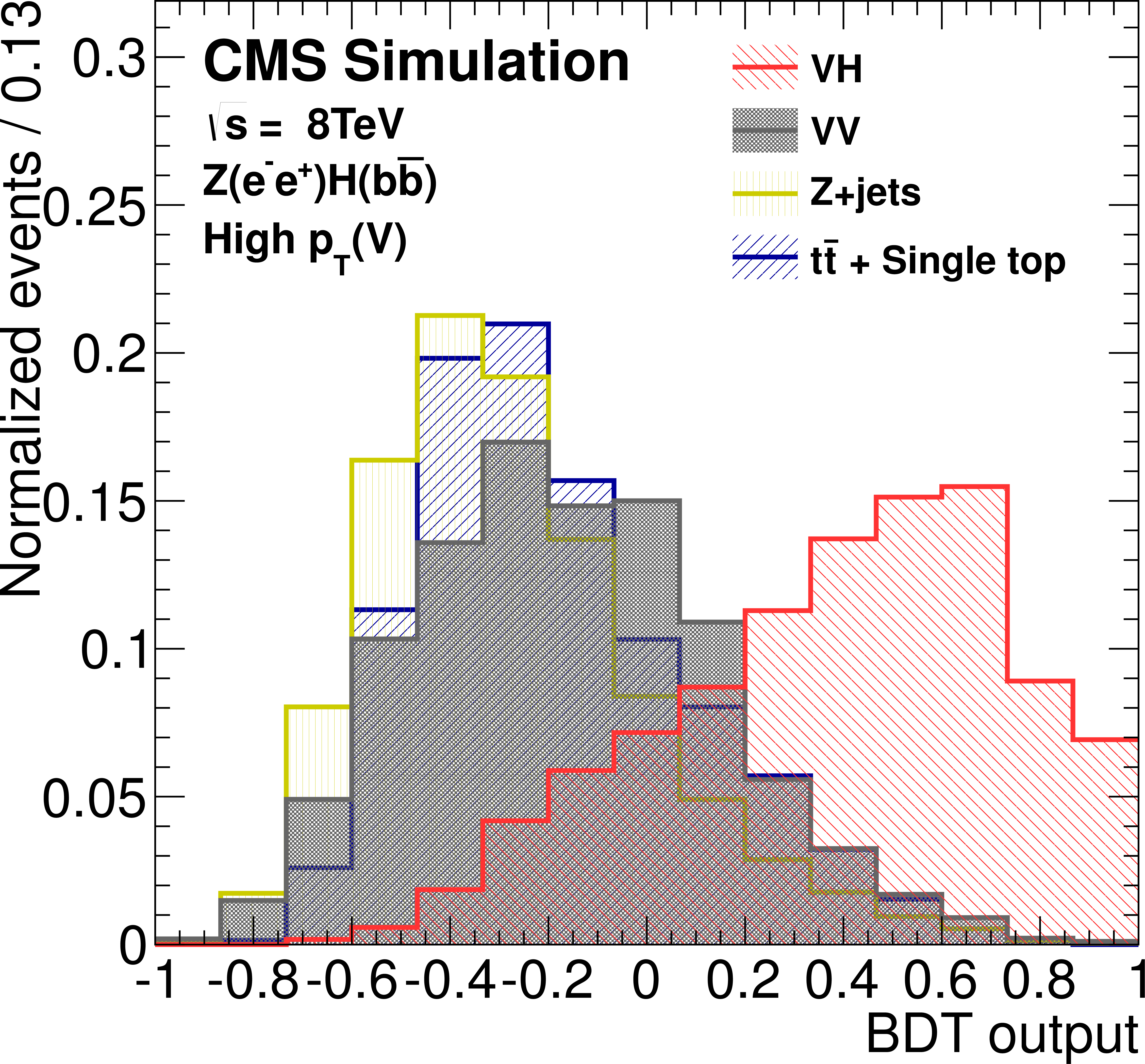
png pdf	Figure 13-a: Post-fit BDT output distributions for $ { {\mathrm {Z}}(\ell \ell ) {\mathrm {H}} } $ in the low-boost region (a, c) and high-boost region (b, d), for 8 TeV data (points with error bars), all backgrounds, and signal, after all selection criteria have been applied. a, b: $ { {\mathrm {Z}}( {{\mu }} {{\mu }}) {\mathrm {H}} } $, c, d: ${ {\mathrm {Z}}( {\mathrm {e}} {\mathrm {e}}) {\mathrm {H}} } $. The bottom inset in each figure shows the ratio of the number of events observed in data to that of the Monte Carlo prediction for signal and backgrounds.
png pdf	Figure 13-b: Post-fit BDT output distributions for $ { {\mathrm {Z}}(\ell \ell ) {\mathrm {H}} } $ in the low-boost region (a, c) and high-boost region (b, d), for 8 TeV data (points with error bars), all backgrounds, and signal, after all selection criteria have been applied. a, b: $ { {\mathrm {Z}}( {{\mu }} {{\mu }}) {\mathrm {H}} } $, c, d: ${ {\mathrm {Z}}( {\mathrm {e}} {\mathrm {e}}) {\mathrm {H}} } $. The bottom inset in each figure shows the ratio of the number of events observed in data to that of the Monte Carlo prediction for signal and backgrounds.
png pdf	Figure 13-c: Post-fit BDT output distributions for $ { {\mathrm {Z}}(\ell \ell ) {\mathrm {H}} } $ in the low-boost region (a, c) and high-boost region (b, d), for 8 TeV data (points with error bars), all backgrounds, and signal, after all selection criteria have been applied. a, b: $ { {\mathrm {Z}}( {{\mu }} {{\mu }}) {\mathrm {H}} } $, c, d: ${ {\mathrm {Z}}( {\mathrm {e}} {\mathrm {e}}) {\mathrm {H}} } $. The bottom inset in each figure shows the ratio of the number of events observed in data to that of the Monte Carlo prediction for signal and backgrounds.
png pdf	Figure 13-d: Post-fit BDT output distributions for $ { {\mathrm {Z}}(\ell \ell ) {\mathrm {H}} } $ in the low-boost region (a, c) and high-boost region (b, d), for 8 TeV data (points with error bars), all backgrounds, and signal, after all selection criteria have been applied. a, b: $ { {\mathrm {Z}}( {{\mu }} {{\mu }}) {\mathrm {H}} } $, c, d: ${ {\mathrm {Z}}( {\mathrm {e}} {\mathrm {e}}) {\mathrm {H}} } $. The bottom inset in each figure shows the ratio of the number of events observed in data to that of the Monte Carlo prediction for signal and backgrounds.
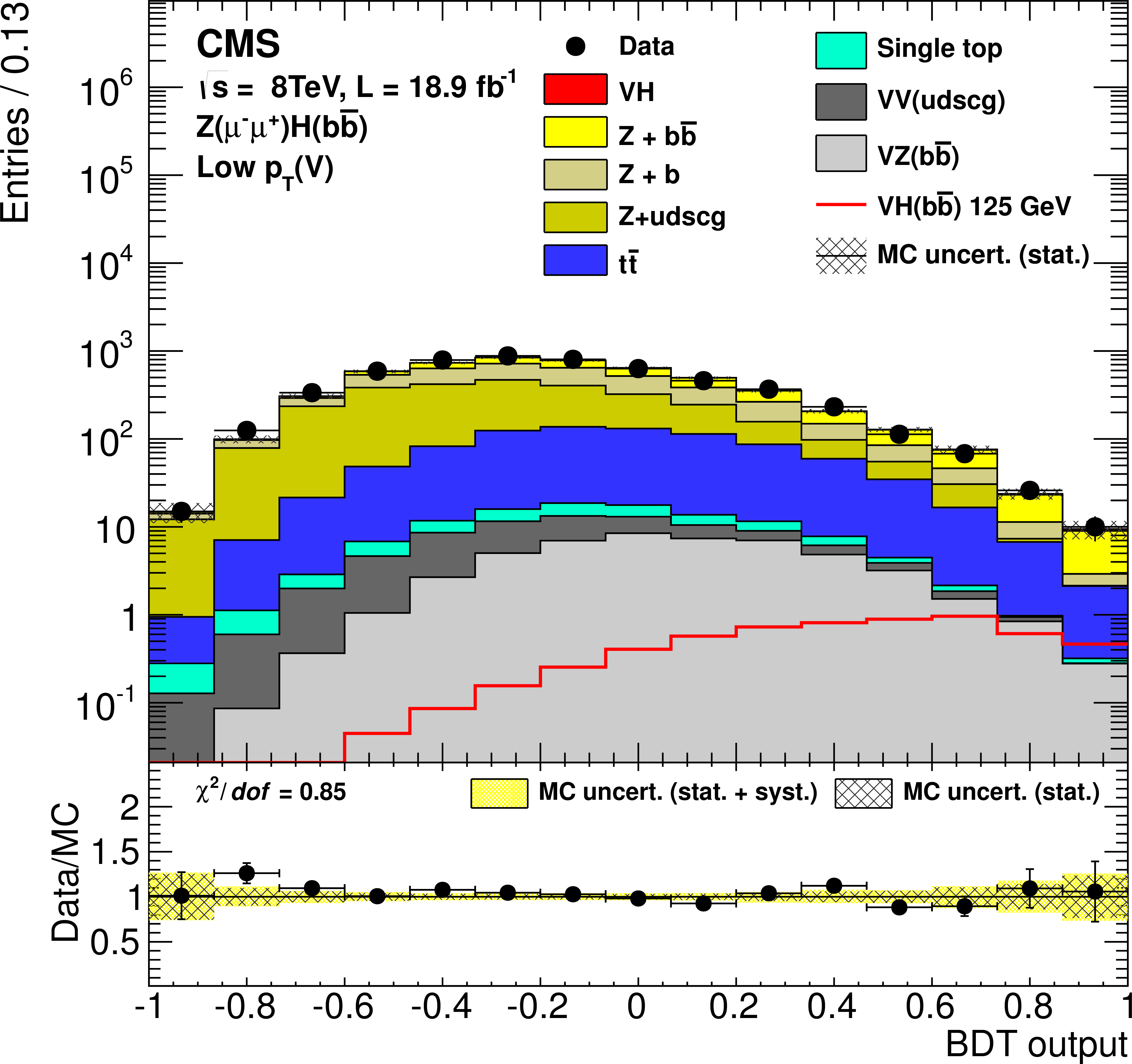
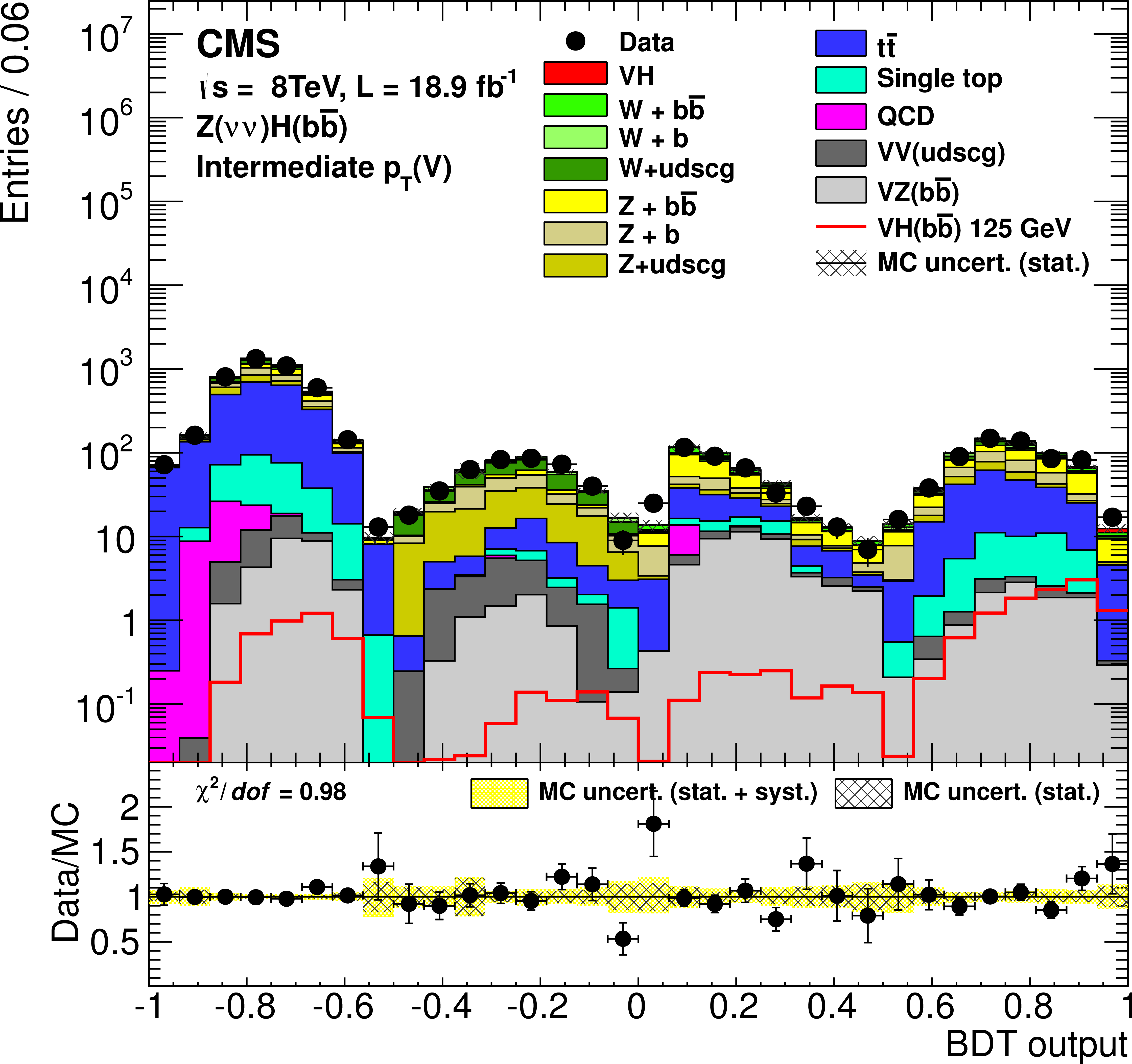
png pdf	Figure 14-a: Post-fit BDT output distributions for $ { {\mathrm {Z}}( {\nu } {\nu }) {\mathrm {H}} } $ in the low-boost region (a), the intermediate-boost (b), and the high-boost (c, d), for 8 TeV data (points with error bars), all backgrounds, and signal, after all selection criteria have been applied. Bottom right: the ${{ {\mathrm {V}} } {\mathrm {H}} } $-enriched partition of the high-boost region is shown in more detail. The bottom inset in each figure shows the ratio of the number of events observed in data to that of the Monte Carlo prediction for signal and backgrounds.
png pdf	Figure 14-b: Post-fit BDT output distributions for $ { {\mathrm {Z}}( {\nu } {\nu }) {\mathrm {H}} } $ in the low-boost region (a), the intermediate-boost (b), and the high-boost (c, d), for 8 TeV data (points with error bars), all backgrounds, and signal, after all selection criteria have been applied. Bottom right: the ${{ {\mathrm {V}} } {\mathrm {H}} } $-enriched partition of the high-boost region is shown in more detail. The bottom inset in each figure shows the ratio of the number of events observed in data to that of the Monte Carlo prediction for signal and backgrounds.
png pdf	Figure 14-c: Post-fit BDT output distributions for $ { {\mathrm {Z}}( {\nu } {\nu }) {\mathrm {H}} } $ in the low-boost region (a), the intermediate-boost (b), and the high-boost (c, d), for 8 TeV data (points with error bars), all backgrounds, and signal, after all selection criteria have been applied. Bottom right: the ${{ {\mathrm {V}} } {\mathrm {H}} } $-enriched partition of the high-boost region is shown in more detail. The bottom inset in each figure shows the ratio of the number of events observed in data to that of the Monte Carlo prediction for signal and backgrounds.
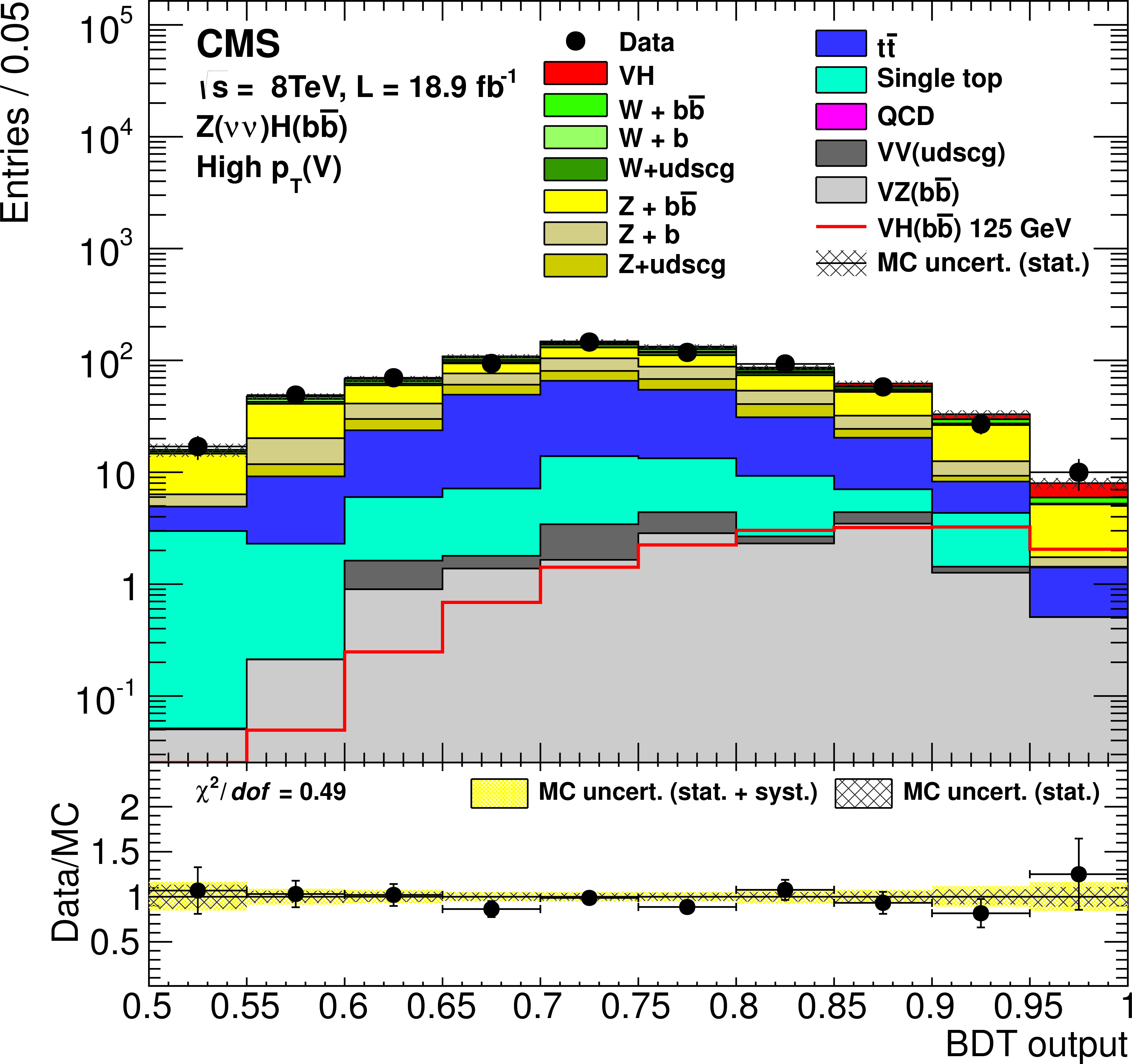
png pdf	Figure 14-d: Post-fit BDT output distributions for $ { {\mathrm {Z}}( {\nu } {\nu }) {\mathrm {H}} } $ in the low-boost region (a), the intermediate-boost (b), and the high-boost (c, d), for 8 TeV data (points with error bars), all backgrounds, and signal, after all selection criteria have been applied. Bottom right: the ${{ {\mathrm {V}} } {\mathrm {H}} } $-enriched partition of the high-boost region is shown in more detail. The bottom inset in each figure shows the ratio of the number of events observed in data to that of the Monte Carlo prediction for signal and backgrounds.
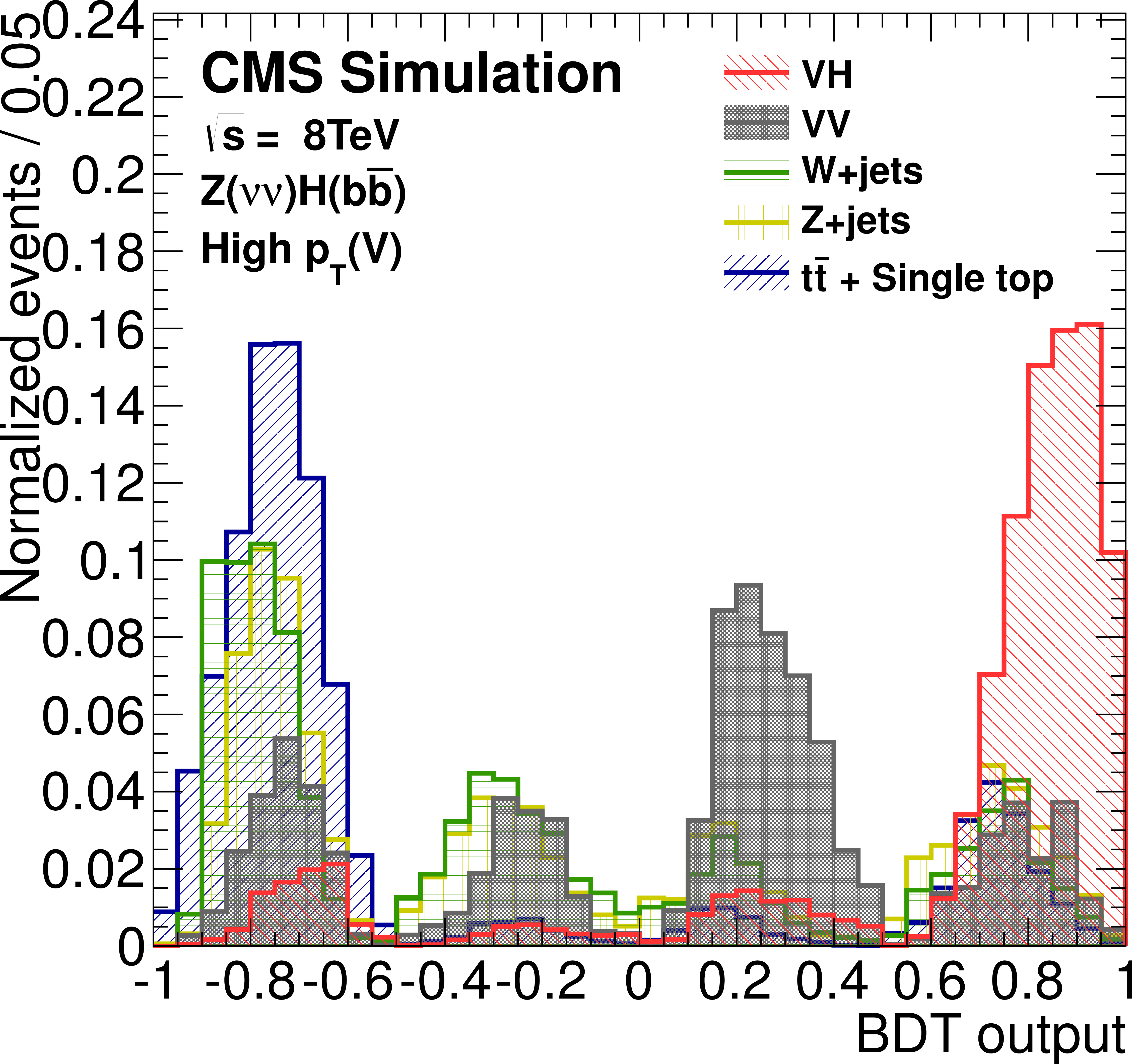
png pdf	Figure 15-a: BDT output distributions, normalized to unity, for the highest-boost region in each channel, for all backgrounds and signal, after all selection criteria have been applied.
png pdf	Figure 15-b: BDT output distributions, normalized to unity, for the highest-boost region in each channel, for all backgrounds and signal, after all selection criteria have been applied.
png pdf	Figure 15-c: BDT output distributions, normalized to unity, for the highest-boost region in each channel, for all backgrounds and signal, after all selection criteria have been applied.
png pdf	Figure 15-d: BDT output distributions, normalized to unity, for the highest-boost region in each channel, for all backgrounds and signal, after all selection criteria have been applied.
png pdf	Figure 15-e: BDT output distributions, normalized to unity, for the highest-boost region in each channel, for all backgrounds and signal, after all selection criteria have been applied.
png pdf	Figure 15-f: BDT output distributions, normalized to unity, for the highest-boost region in each channel, for all backgrounds and signal, after all selection criteria have been applied.