

Compact Muon Solenoid
LHC, CERN
| CMS-HIG-13-024 ; CERN-PH-EP-2015-148 | ||
| Search for neutral MSSM Higgs bosons decaying to $\mu^{+} \mu^{-}$ in pp collisions at $ \sqrt{s} =$ 7 and 8 TeV | ||
| CMS Collaboration | ||
| 6 August 2015 | ||
| Phys. Lett. B 752 (2016) 221 | ||
| Abstract: A search for neutral Higgs bosons predicted in the minimal supersymmetric standard model (MSSM) for $\mu^{+} \mu^{-}$ decay channels is presented. The analysis uses data collected by the CMS experiment at the LHC in proton-proton collisions at centre-of-mass energies of 7 and 8 TeV, corresponding to integrated luminosities of 5.1 and 19.3 fb$^{-1}$, respectively. The search is sensitive to Higgs bosons produced through the gluon fusion process and in association with a bb quark pair. No statistically significant excess is observed in the $\mu^{+} \mu^{-}$ mass spectrum. Results are interpreted in the framework of several benchmark scenarios, and the data are used to set an upper limit on the MSSM parameter $ \tan{ \beta} $ as a function of the mass of the pseudoscalar A boson in the range from 115 to 300 GeV. Model independent upper limits are given for the product of the cross section and branching fraction for gluon fusion and b quark associated production. They are the most stringent limits obtained to date in this channel. | ||
| Links: e-print arXiv:1508.01437 [hep-ex] (PDF) ; CDS record ; inSPIRE record ; HepData record ; CADI line (restricted) ; | ||
| Figures | |
png pdf |
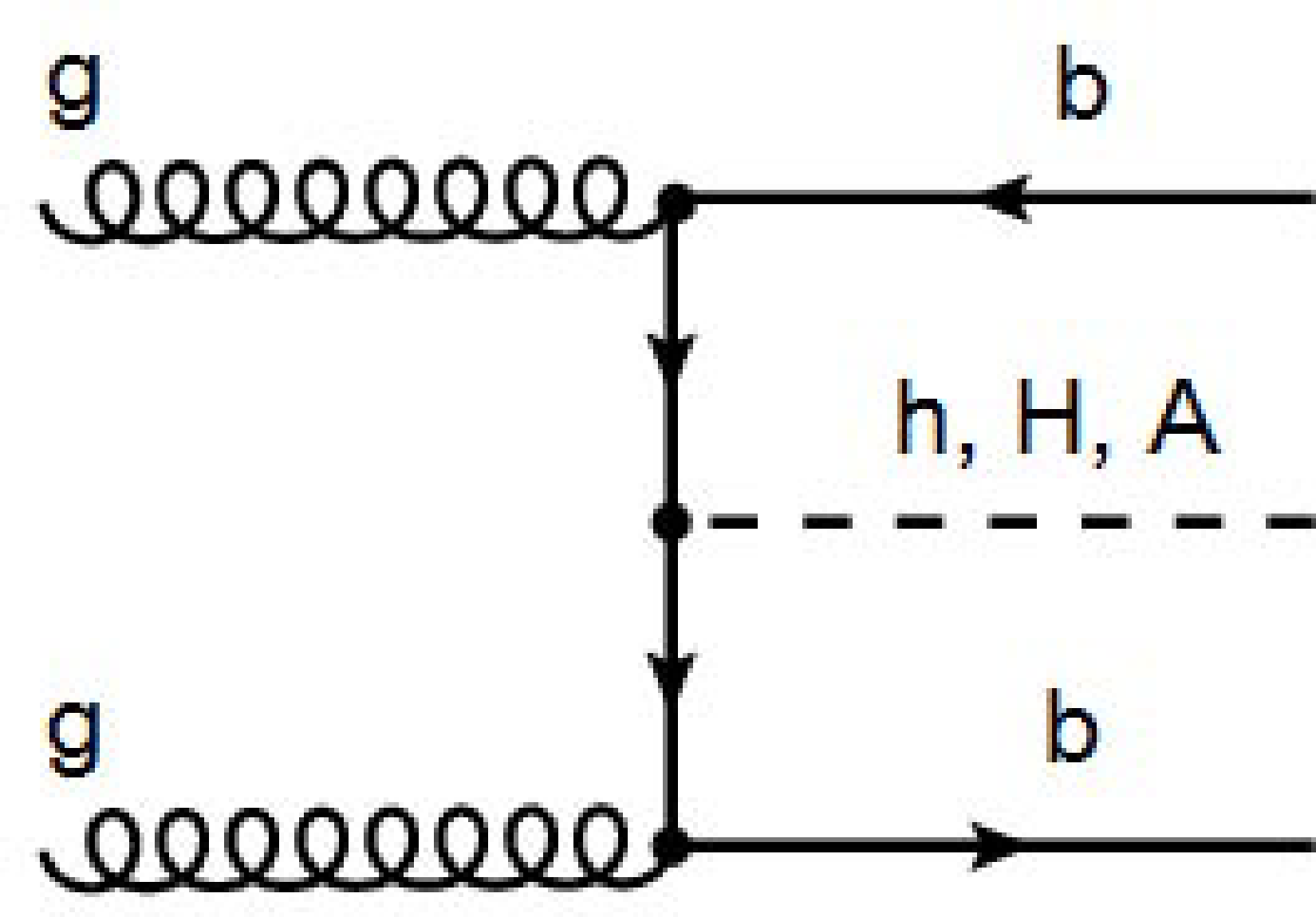
Figure 1-a:
Leading-order diagrams for the main production processes of MSSM Higgs bosons at the LHC (a) in association with $ { {\mathrm {b}} {\overline {\mathrm {b}}} } $ production and (b) through gluon fusion. |
png pdf |
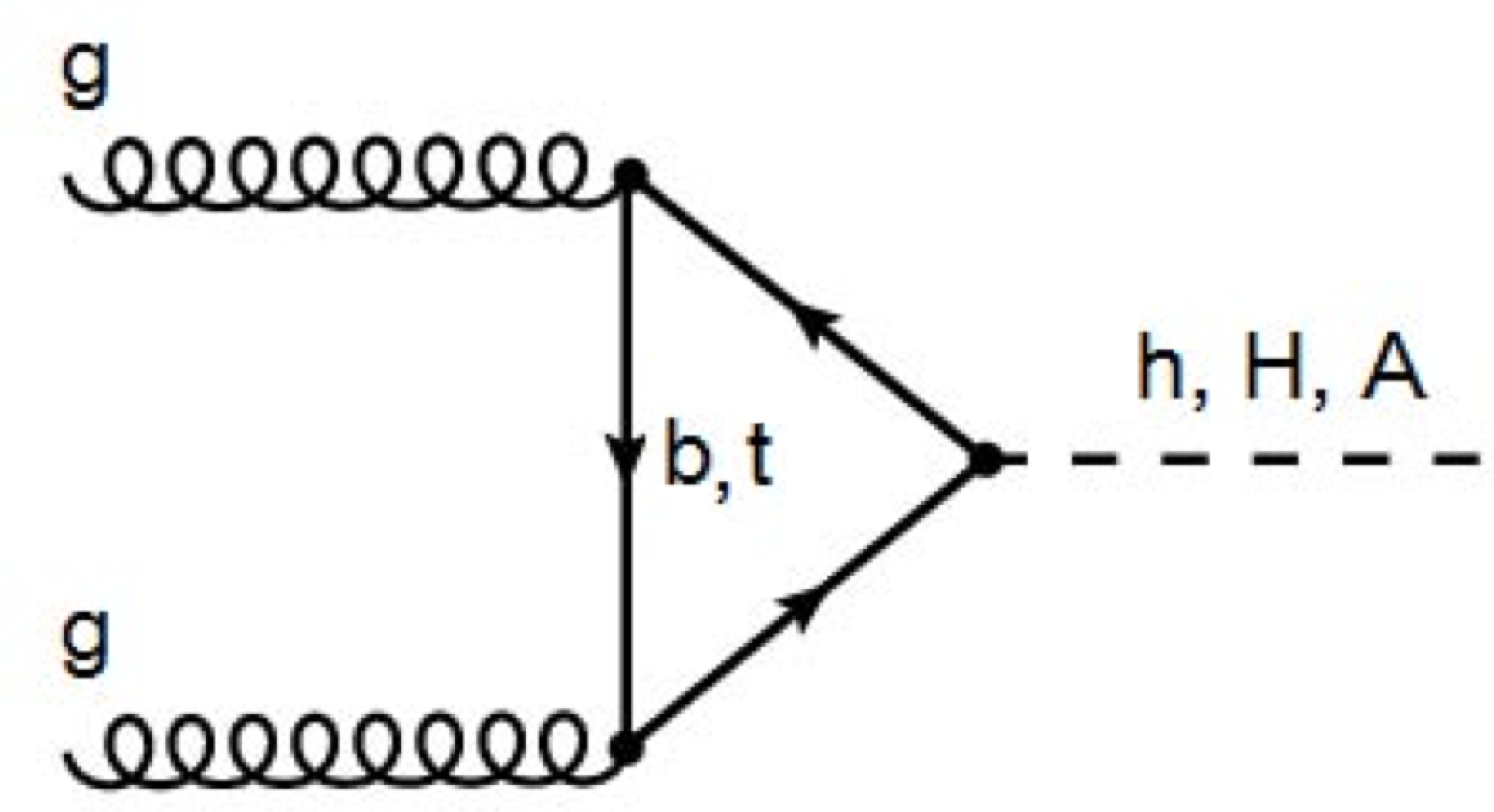
Figure 1-b:
Leading-order diagrams for the main production processes of MSSM Higgs bosons at the LHC (a) in association with $ { {\mathrm {b}} {\overline {\mathrm {b}}} } $ production and (b) through gluon fusion. |
png pdf |
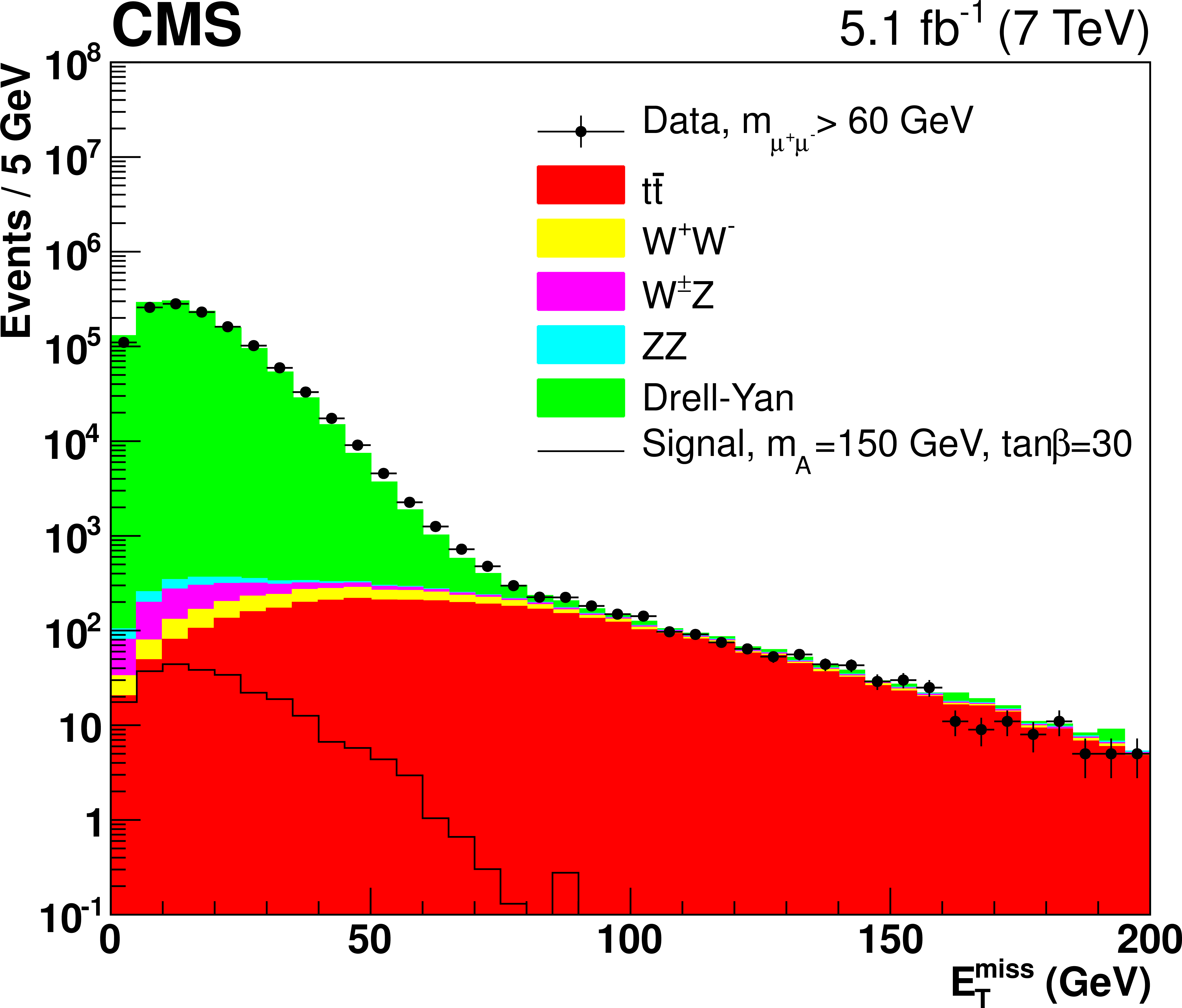
Figure 2-a:
The $ {E_{\mathrm {T}}^{\text {miss}}} $ distribution with a reconstructed dimuon invariant mass $m_{ {\mu ^+} {\mu ^-} }>$ 60 GeV in data and in simulated events at $\sqrt {s}=$ 7 (a) and $\sqrt {s}=$ 8 TeV (b). The expected contribution is also shown for the signal at $m_{ {\mathrm {A}} }=$ 150 GeV and $\tan \beta =$ 30. |
png pdf |
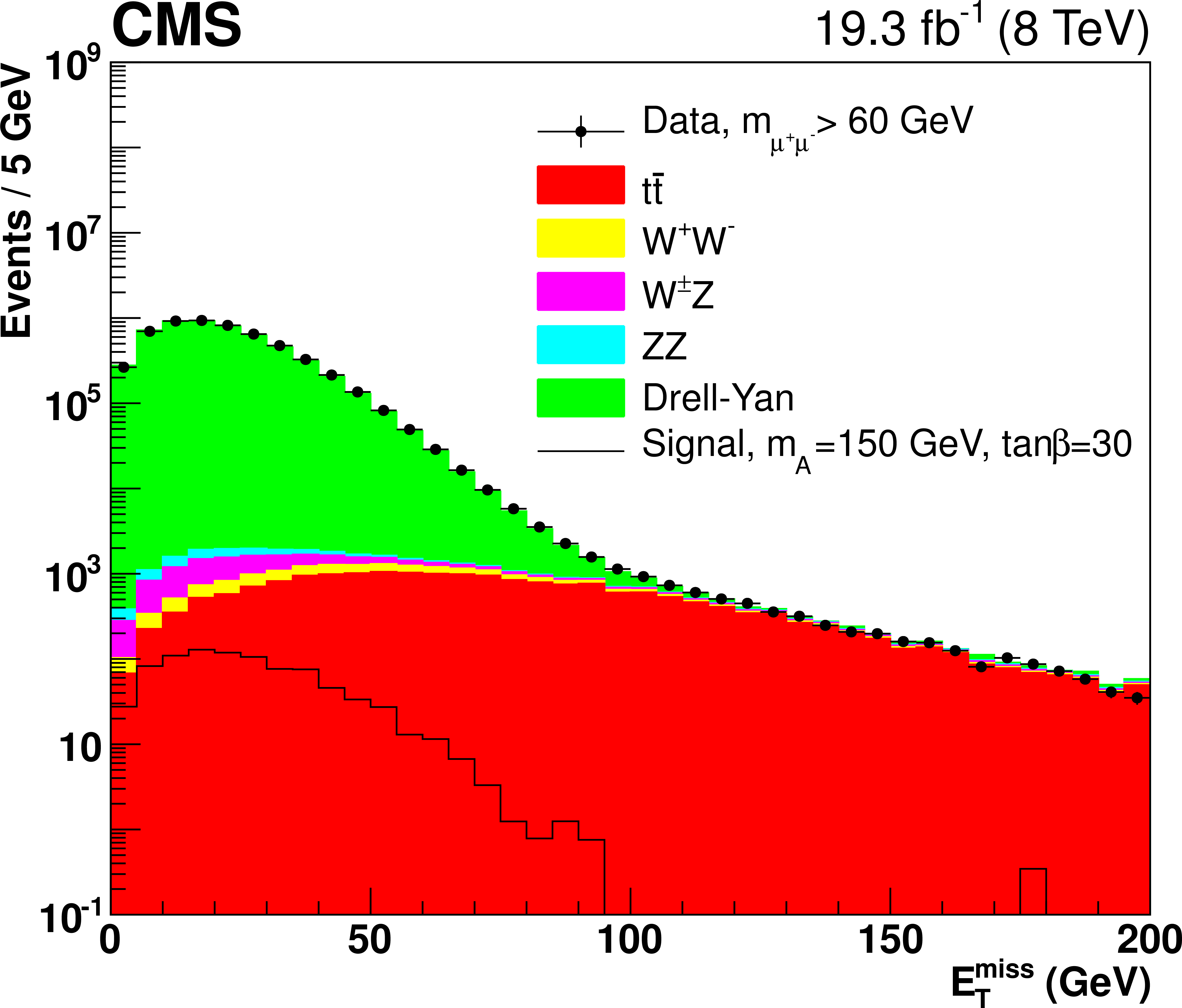
Figure 2-b:
The $ {E_{\mathrm {T}}^{\text {miss}}} $ distribution with a reconstructed dimuon invariant mass $m_{ {\mu ^+} {\mu ^-} }>$ 60 GeV in data and in simulated events at $\sqrt {s}=$ 7 (a) and $\sqrt {s}=$ 8 TeV (b). The expected contribution is also shown for the signal at $m_{ {\mathrm {A}} }=$ 150 GeV and $\tan \beta =$ 30. |
png pdf |
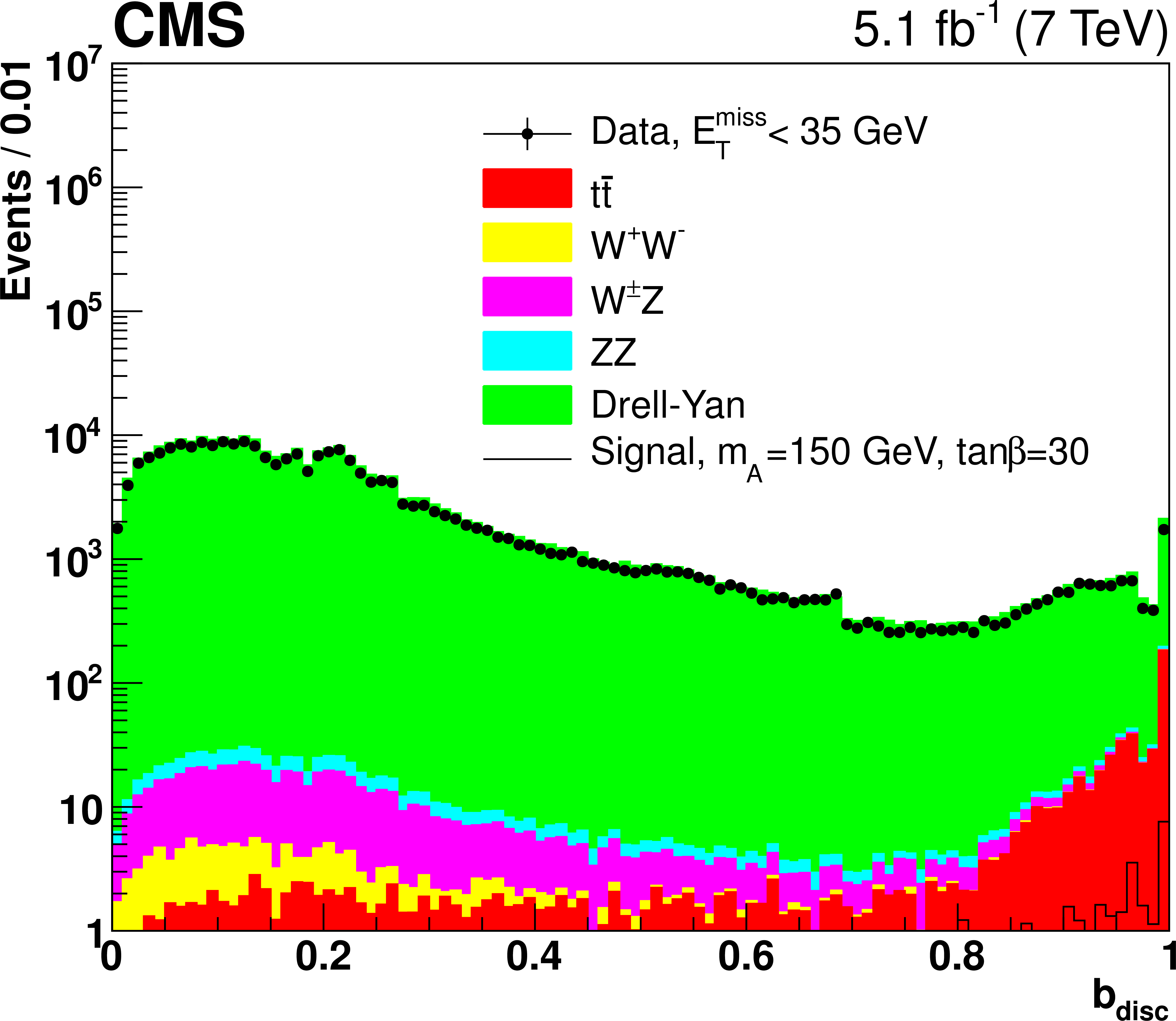
Figure 3-a:
The distribution of the b tagging discriminant, $b_\mathrm {disc}$, for events that satisfy the selection $ {E_{\mathrm {T}}^{\text {miss}}} <$ 35 GeV in data collected at $\sqrt {s}=$ 7 (a) and $\sqrt {s}=$ 8 TeV (b). For each event, the largest value of $b_\mathrm {disc}$ is selected. |
png pdf |
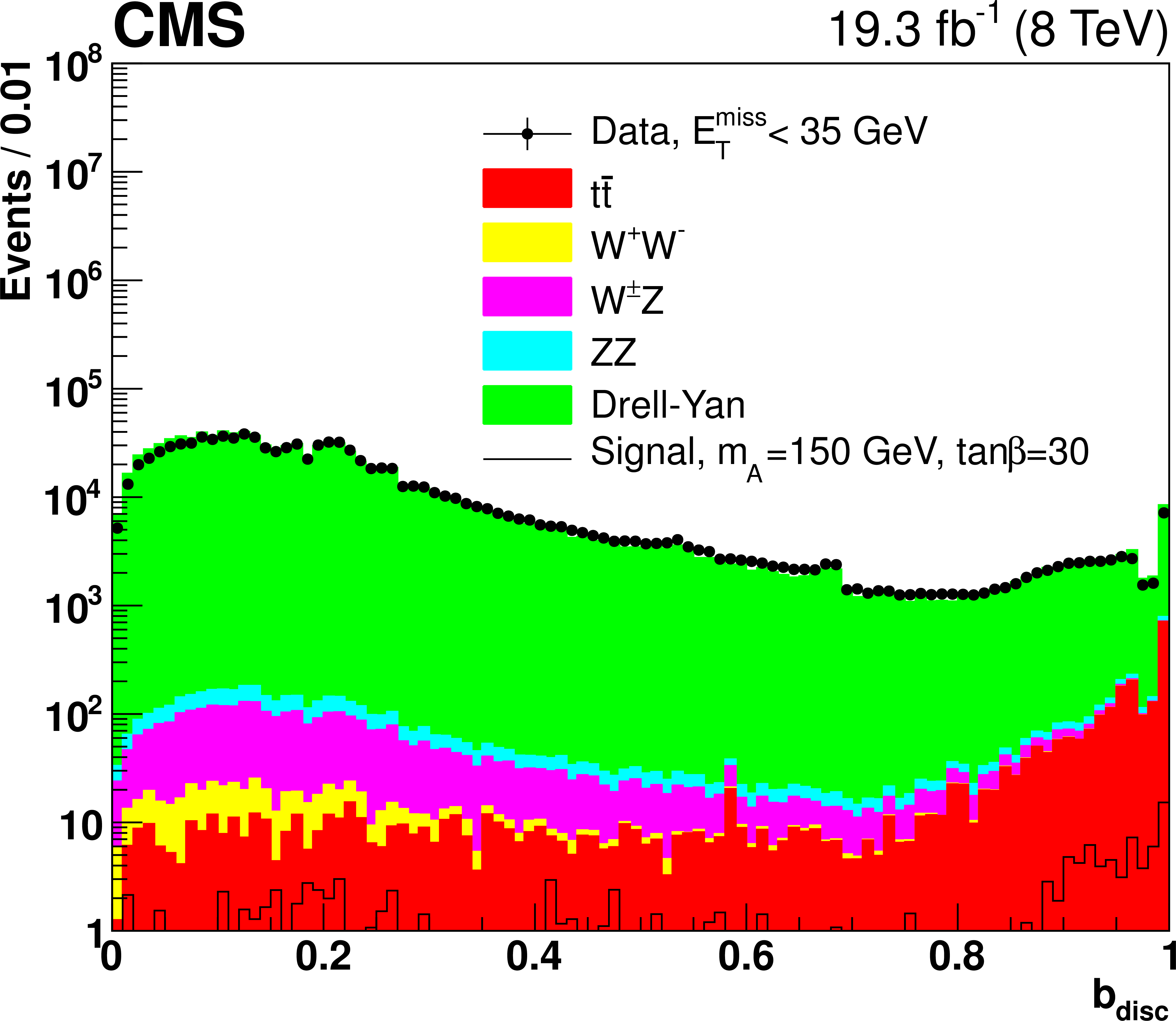
Figure 3-b:
The distribution of the b tagging discriminant, $b_\mathrm {disc}$, for events that satisfy the selection $ {E_{\mathrm {T}}^{\text {miss}}} <$ 35 GeV in data collected at $\sqrt {s}=$ 7 (a) and $\sqrt {s}=$ 8 TeV (b). For each event, the largest value of $b_\mathrm {disc}$ is selected. |
png pdf |
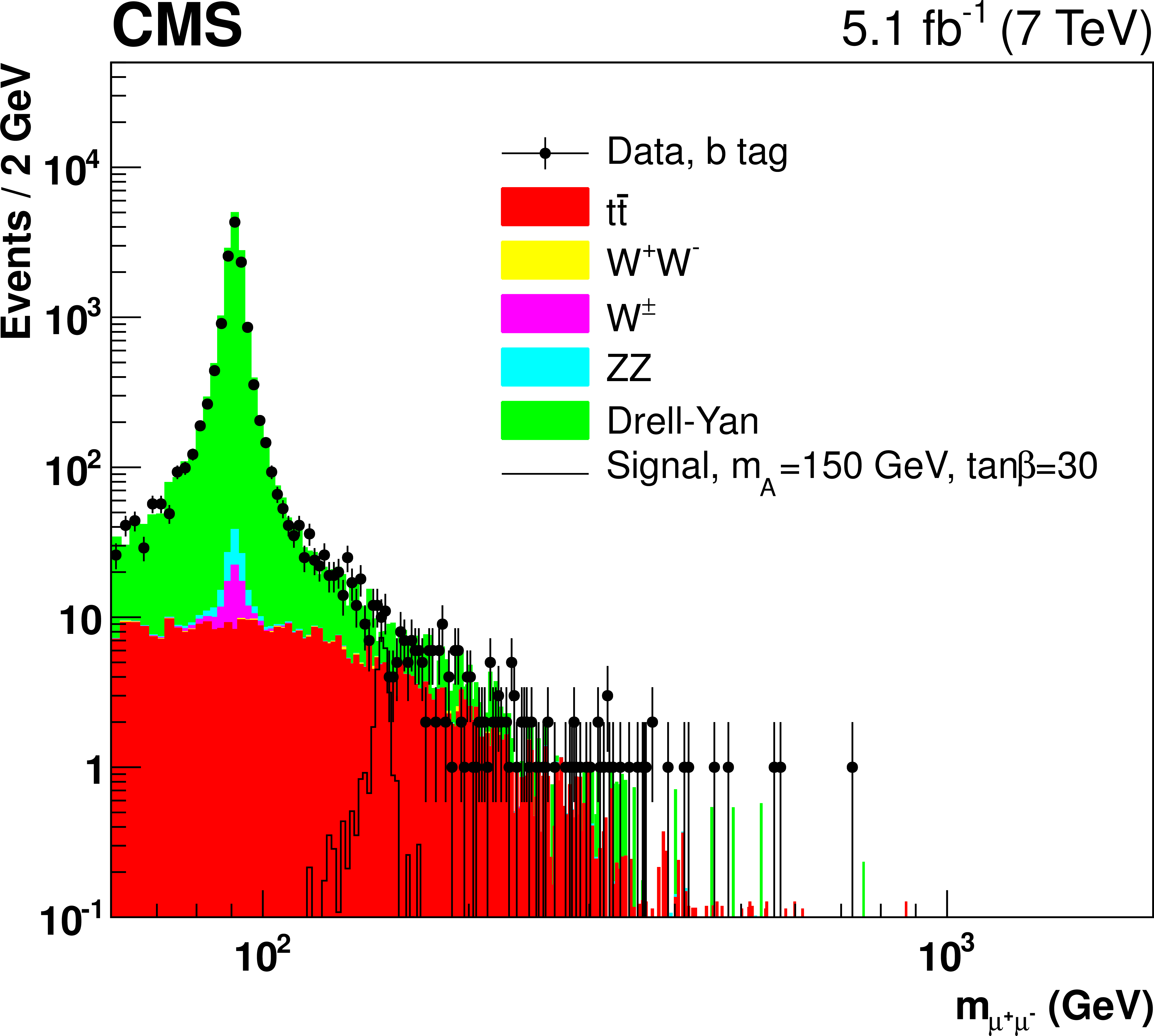
Figure 4-a:
The dimuon invariant mass distribution for events that belong to C1 (a) and C2 category (b), for data and simulated events at $\sqrt {s}=$ 7 TeV. The corresponding quantities are shown for $\sqrt {s} = $ 8 TeV (c and d). The expected contributions to signal assuming the $m_{ {\mathrm {h}} }^\mathrm {mod +}$ scenario for $m_{ {\mathrm {A}} }=$ 150 GeV and $\tan \beta =$ 30 are displayed for comparison. |
png pdf |
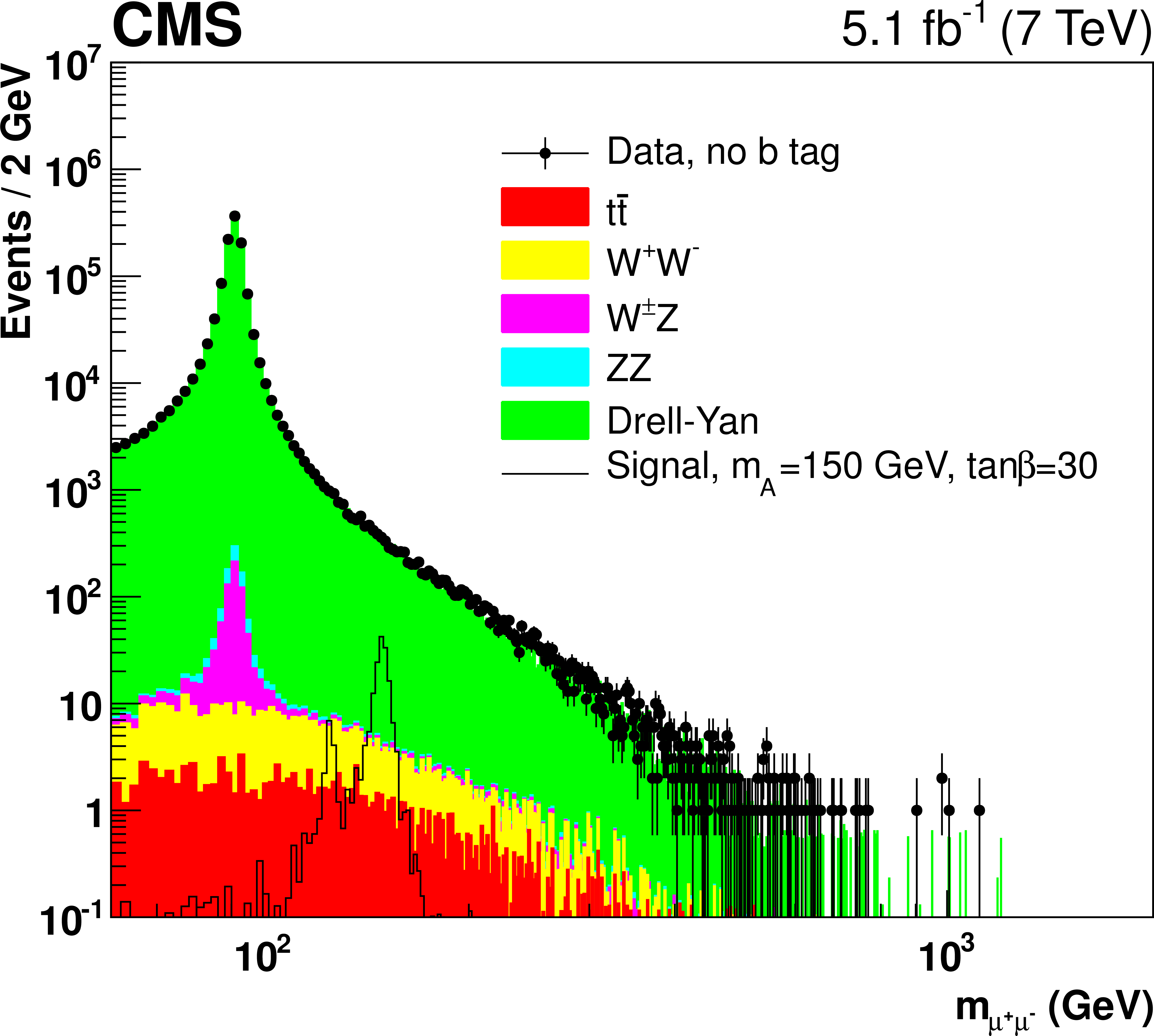
Figure 4-b:
The dimuon invariant mass distribution for events that belong to C1 (a) and C2 category (b), for data and simulated events at $\sqrt {s}=$ 7 TeV. The corresponding quantities are shown for $\sqrt {s} = $ 8 TeV (c and d). The expected contributions to signal assuming the $m_{ {\mathrm {h}} }^\mathrm {mod +}$ scenario for $m_{ {\mathrm {A}} }=$ 150 GeV and $\tan \beta =$ 30 are displayed for comparison. |

png pdf |
Figure 4-c:
The dimuon invariant mass distribution for events that belong to C1 (a) and C2 category (b), for data and simulated events at $\sqrt {s}=$ 7 TeV. The corresponding quantities are shown for $\sqrt {s} = $ 8 TeV (c and d). The expected contributions to signal assuming the $m_{ {\mathrm {h}} }^\mathrm {mod +}$ scenario for $m_{ {\mathrm {A}} }=$ 150 GeV and $\tan \beta =$ 30 are displayed for comparison. |
png pdf |
Figure 4-d:
The dimuon invariant mass distribution for events that belong to C1 (a) and C2 category (b), for data and simulated events at $\sqrt {s}=$ 7 TeV. The corresponding quantities are shown for $\sqrt {s} = $ 8 TeV (c and d). The expected contributions to signal assuming the $m_{ {\mathrm {h}} }^\mathrm {mod +}$ scenario for $m_{ {\mathrm {A}} }=$ 150 GeV and $\tan \beta =$ 30 are displayed for comparison. |

png pdf |
Figure 5-a:
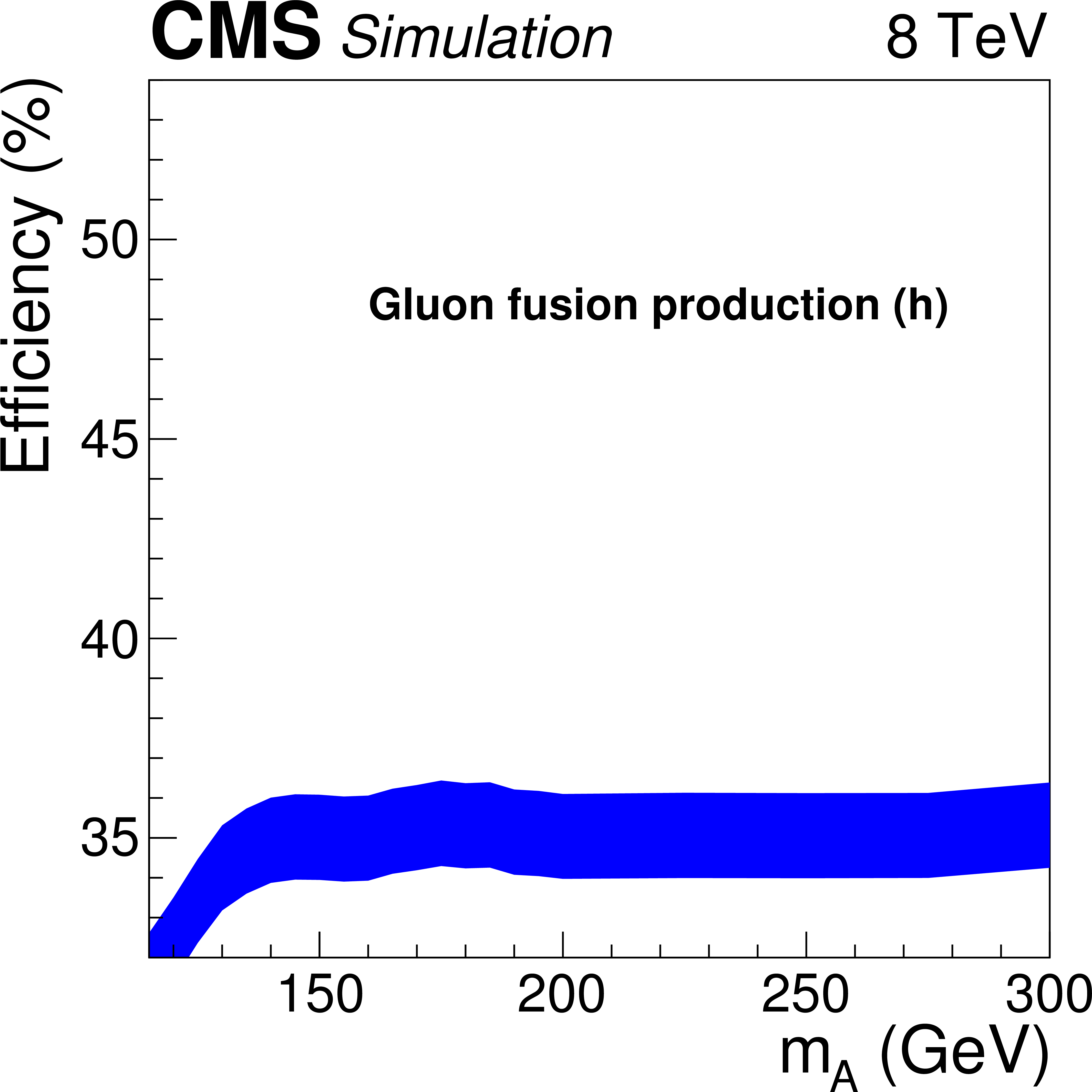
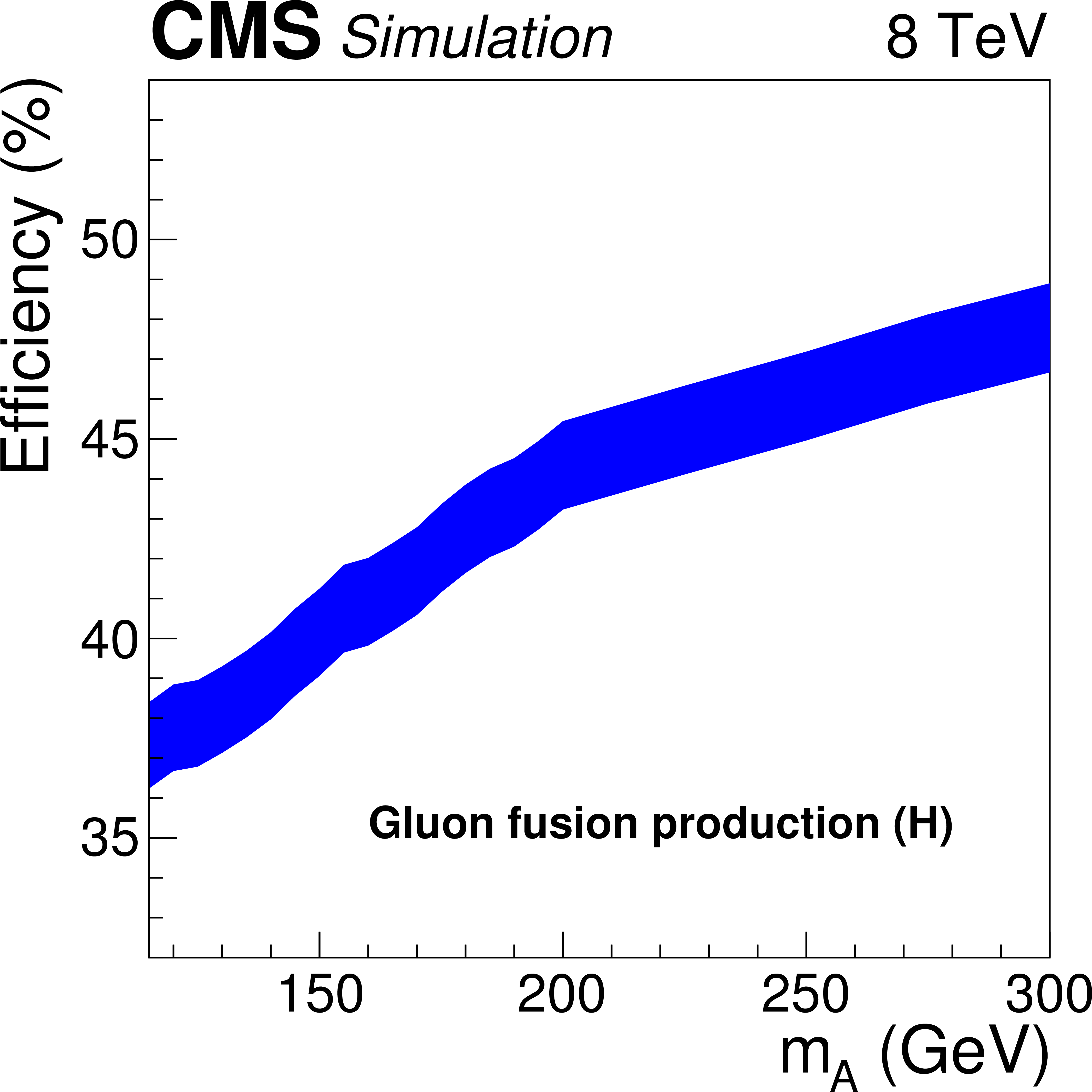
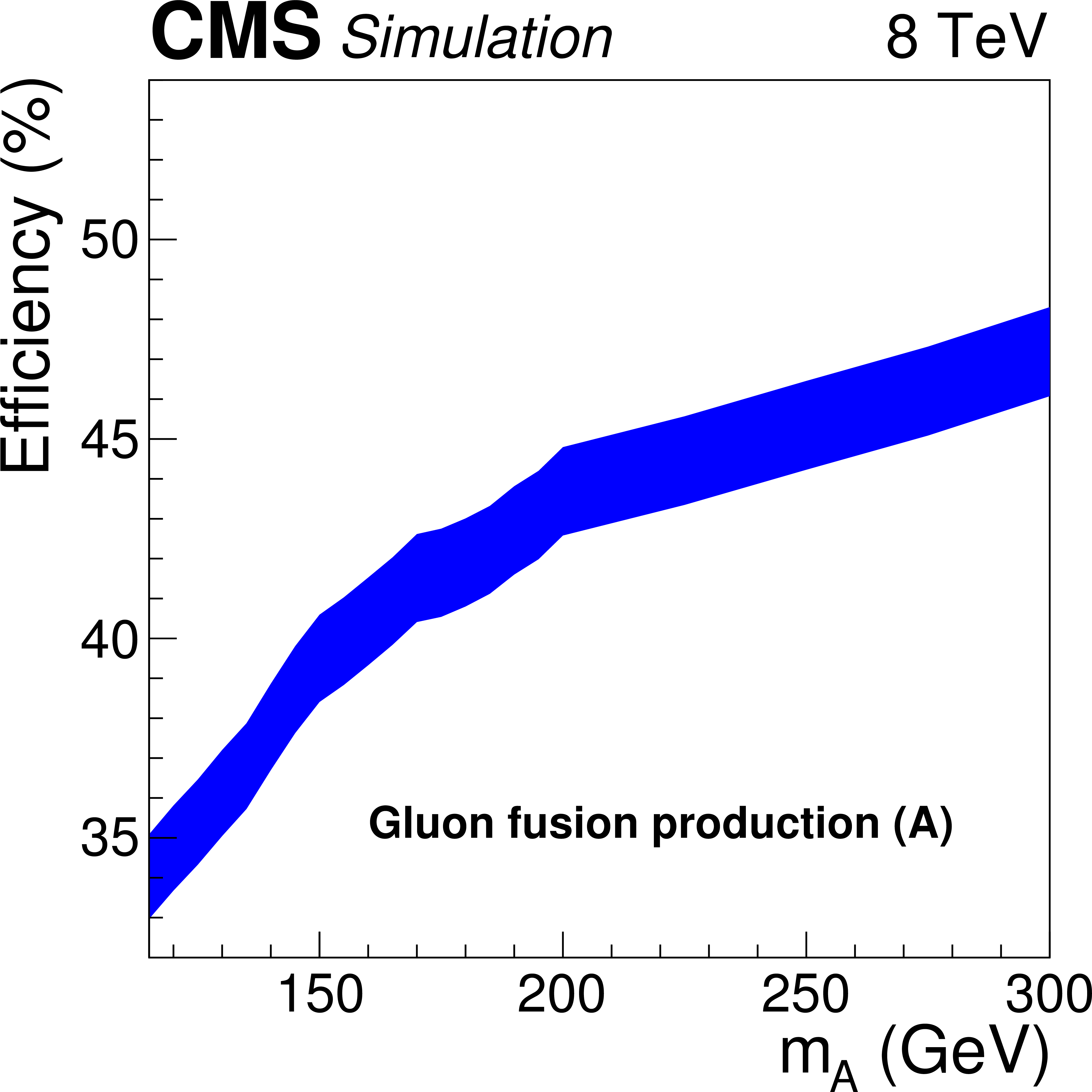
Signal efficiency for the AP process at $\sqrt {s}=$ 8 TeV, shown separately for the three $\phi $ boson types, (a) $ {\mathrm {h}} $, (b) $ {\mathrm {H}} $ and (c) $ {\mathrm {A}} $, as a function of $m_{ {\mathrm {A}} }$. The corresponding efficiency for the GF production process is shown in the lower row. The contributions from the two event categories C1 and C2 are combined. The results are integrated over $\tan \beta $, since the efficiency does not strongly depend on this quantity. The band shows the change in efficiency due to the limited statistics of the MC samples. |

png pdf |
Figure 5-b:
Signal efficiency for the AP process at $\sqrt {s}=$ 8 TeV, shown separately for the three $\phi $ boson types, (a) $ {\mathrm {h}} $, (b) $ {\mathrm {H}} $ and (c) $ {\mathrm {A}} $, as a function of $m_{ {\mathrm {A}} }$. The corresponding efficiency for the GF production process is shown in the lower row. The contributions from the two event categories C1 and C2 are combined. The results are integrated over $\tan \beta $, since the efficiency does not strongly depend on this quantity. The band shows the change in efficiency due to the limited statistics of the MC samples. |
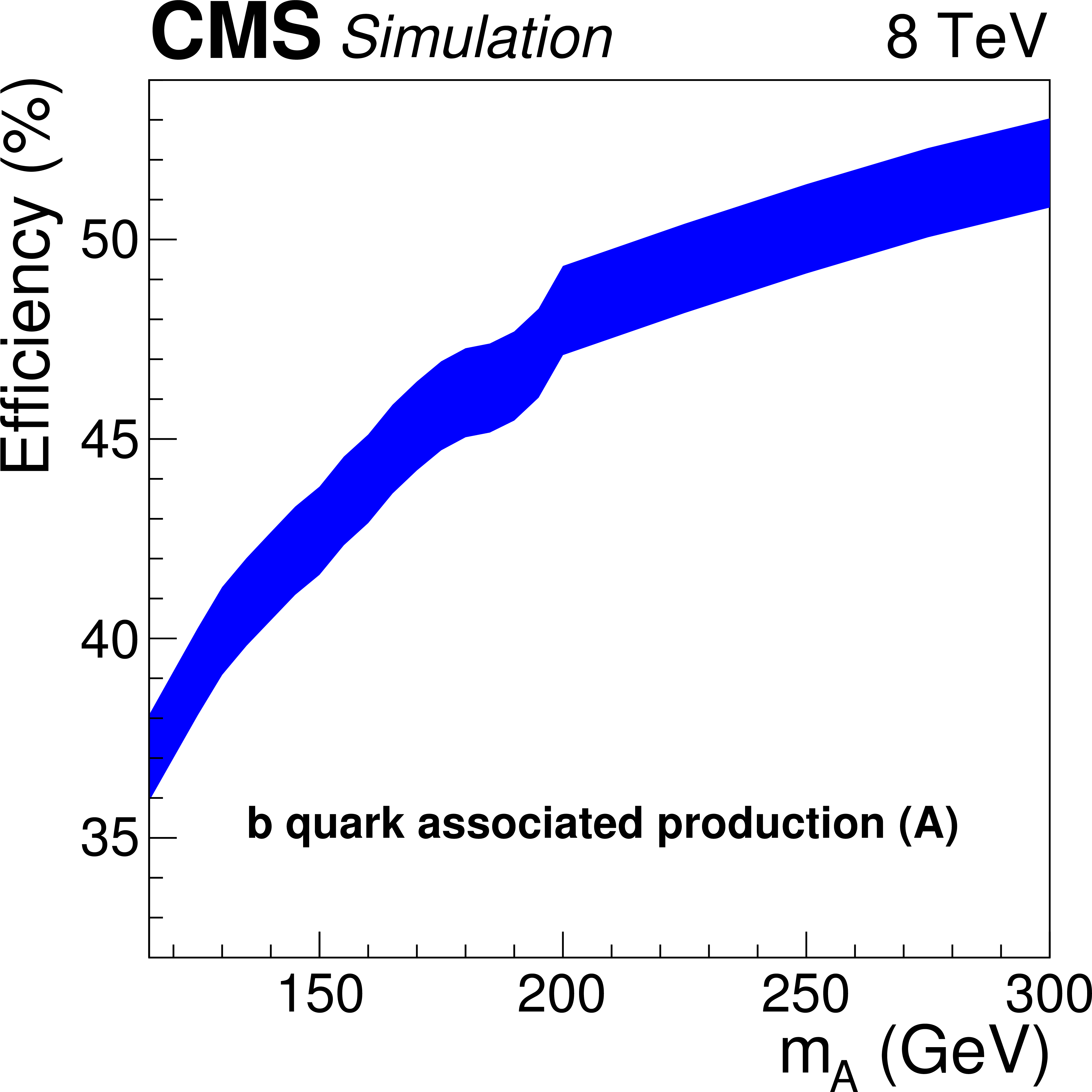
png pdf |
Figure 5-c:
Signal efficiency for the AP process at $\sqrt {s}=$ 8 TeV, shown separately for the three $\phi $ boson types, (a) $ {\mathrm {h}} $, (b) $ {\mathrm {H}} $ and (c) $ {\mathrm {A}} $, as a function of $m_{ {\mathrm {A}} }$. The corresponding efficiency for the GF production process is shown in the lower row. The contributions from the two event categories C1 and C2 are combined. The results are integrated over $\tan \beta $, since the efficiency does not strongly depend on this quantity. The band shows the change in efficiency due to the limited statistics of the MC samples. |
png pdf |
Figure 5-d:
Signal efficiency for the AP process at $\sqrt {s}=$ 8 TeV, shown separately for the three $\phi $ boson types, (a) $ {\mathrm {h}} $, (b) $ {\mathrm {H}} $ and (c) $ {\mathrm {A}} $, as a function of $m_{ {\mathrm {A}} }$. The corresponding efficiency for the GF production process is shown in the lower row. The contributions from the two event categories C1 and C2 are combined. The results are integrated over $\tan \beta $, since the efficiency does not strongly depend on this quantity. The band shows the change in efficiency due to the limited statistics of the MC samples. |
png pdf |
Figure 5-e:
Signal efficiency for the AP process at $\sqrt {s}=$ 8 TeV, shown separately for the three $\phi $ boson types, (a) $ {\mathrm {h}} $, (b) $ {\mathrm {H}} $ and (c) $ {\mathrm {A}} $, as a function of $m_{ {\mathrm {A}} }$. The corresponding efficiency for the GF production process is shown in the lower row. The contributions from the two event categories C1 and C2 are combined. The results are integrated over $\tan \beta $, since the efficiency does not strongly depend on this quantity. The band shows the change in efficiency due to the limited statistics of the MC samples. |
png pdf |
Figure 5-f:
Signal efficiency for the AP process at $\sqrt {s}=$ 8 TeV, shown separately for the three $\phi $ boson types, (a) $ {\mathrm {h}} $, (b) $ {\mathrm {H}} $ and (c) $ {\mathrm {A}} $, as a function of $m_{ {\mathrm {A}} }$. The corresponding efficiency for the GF production process is shown in the lower row. The contributions from the two event categories C1 and C2 are combined. The results are integrated over $\tan \beta $, since the efficiency does not strongly depend on this quantity. The band shows the change in efficiency due to the limited statistics of the MC samples. |
png pdf |
Figure 6-a:
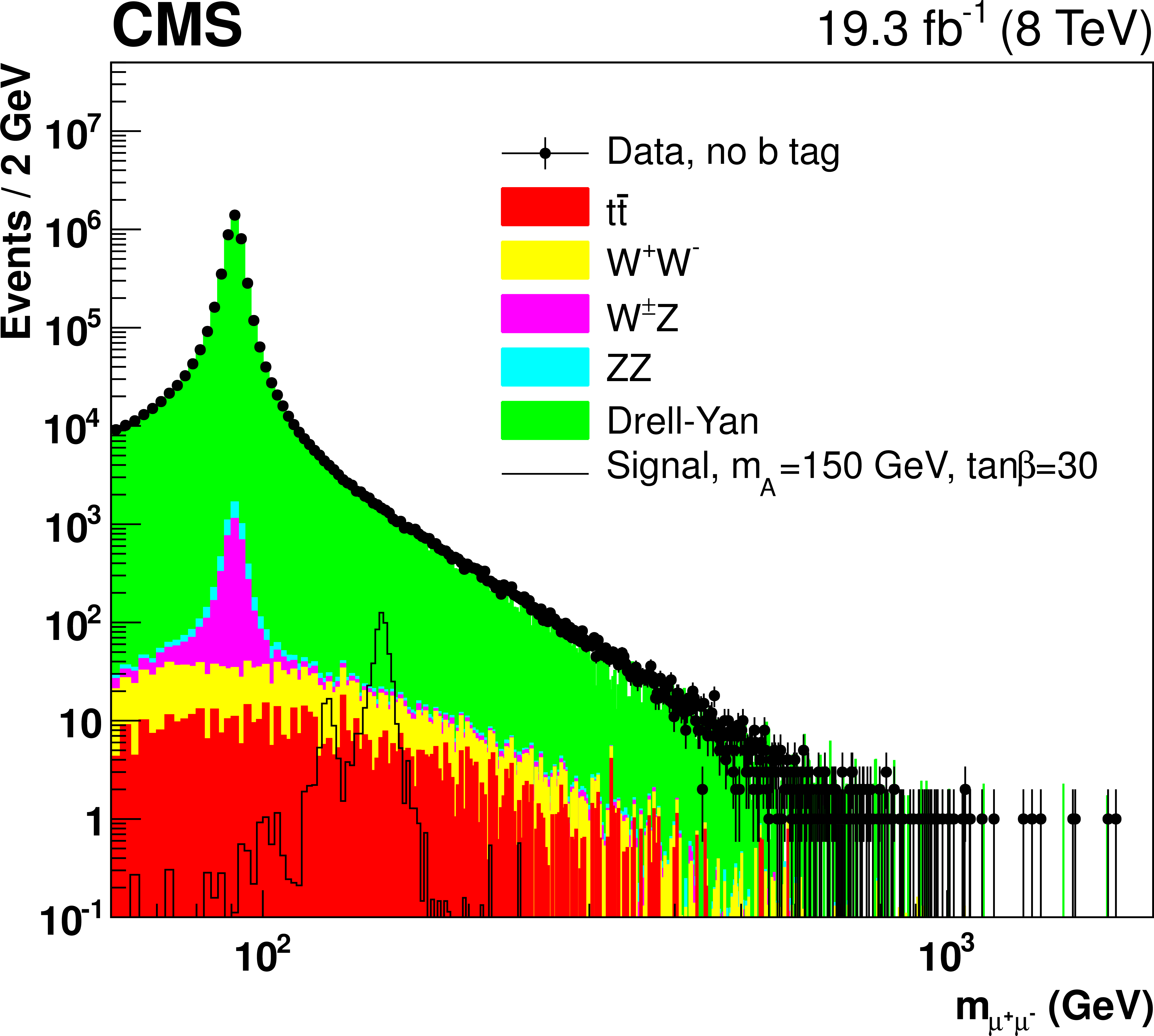
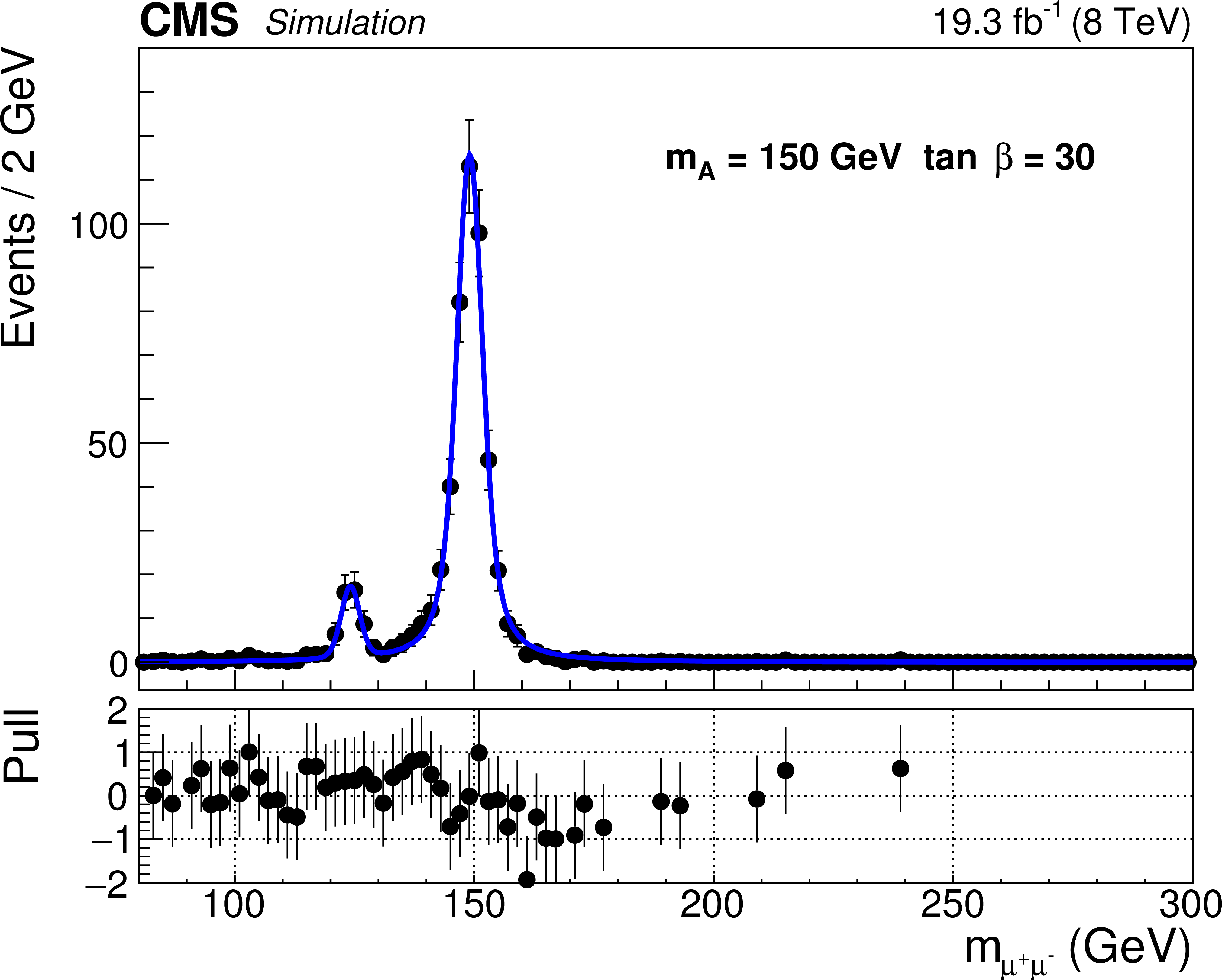
Invariant mass distribution of the expected signal for $m_{ {\mathrm {A}} }=$ 150 GeV and $ \tan\beta =$ 30 (a), and an example of the fit to the data at $\sqrt {s}=8 TeV $ including the same signal assumption (b). The distribution represents the expected number of events for an integrated luminosity of 19.3fb$^{-1}$. For each plot the pull of the fit as a function of the dimuon invariant mass is shown. |
png pdf |
Figure 6-b:
Invariant mass distribution of the expected signal for $m_{ {\mathrm {A}} }=$ 150 GeV and $ \tan\beta =$ 30 (a), and an example of the fit to the data at $\sqrt {s}=8 TeV $ including the same signal assumption (b). The distribution represents the expected number of events for an integrated luminosity of 19.3fb$^{-1}$. For each plot the pull of the fit as a function of the dimuon invariant mass is shown. |
png pdf |
Figure 7:
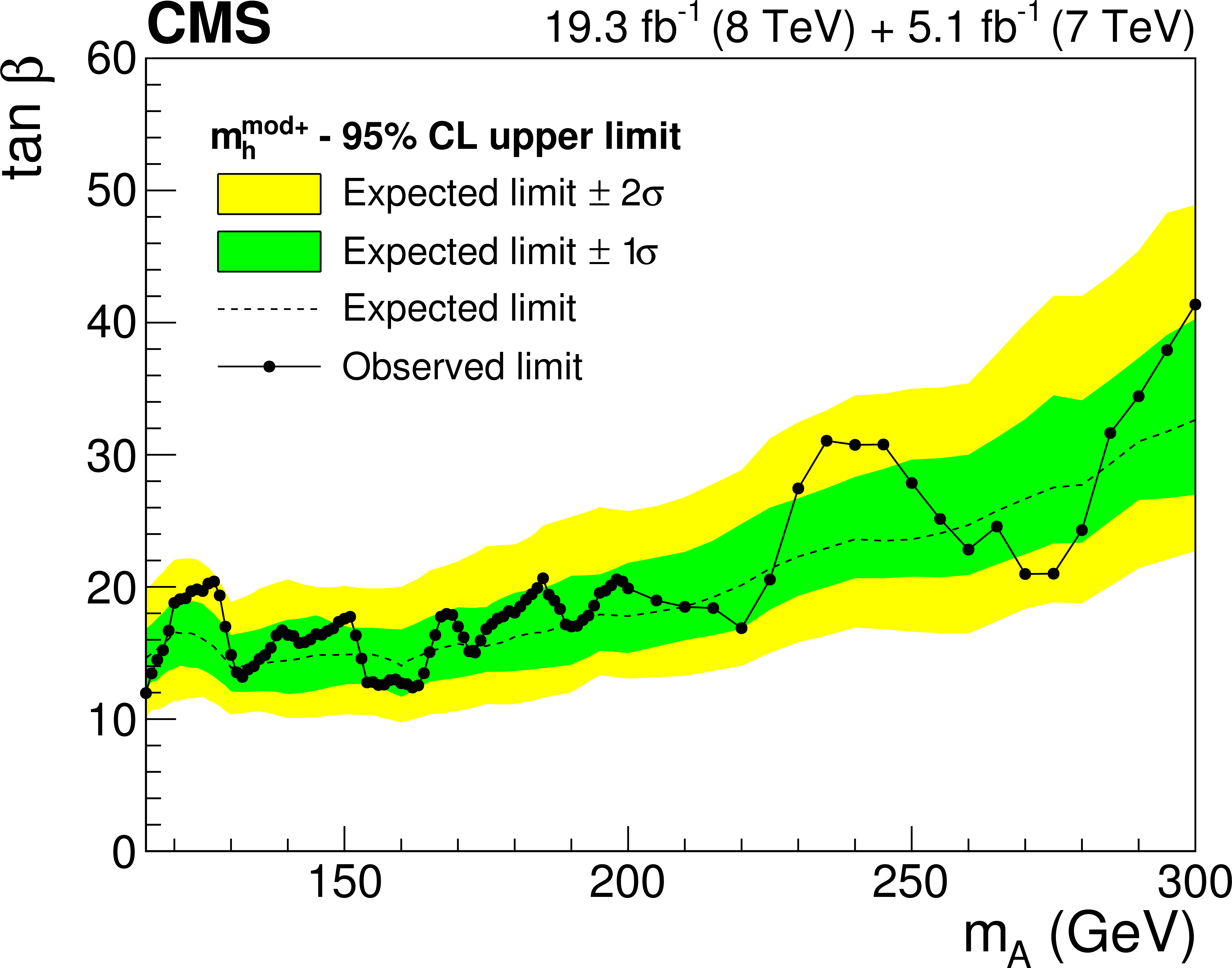
The 95% CL upper limit on $\tan \beta $ as a function of $m_{ {\mathrm {A}} }$, after combining the data from the two event categories at the two centre-of-mass energies (7 and 8 TeV). The results are obtained in the framework of the $m_{ {\mathrm {h}} }^\mathrm {mod +}$ benchmark scenario. |

png pdf |
Figure 8:
Comparison of the 95% CL exclusion limits on $\tan \beta $ obtained within MSSM benchmark models, as a function of $m_{ {\mathrm {A}} }$. The quantity $\Delta \tan \beta = \tan \beta_{m_{ {\mathrm {h}} }^\mathrm {mod +}} - \tan \beta _\text {scenario}$ represents the difference in $ \tan \beta $ at which the 95% CL limit is obtained for alternative scenarios. |
png pdf |
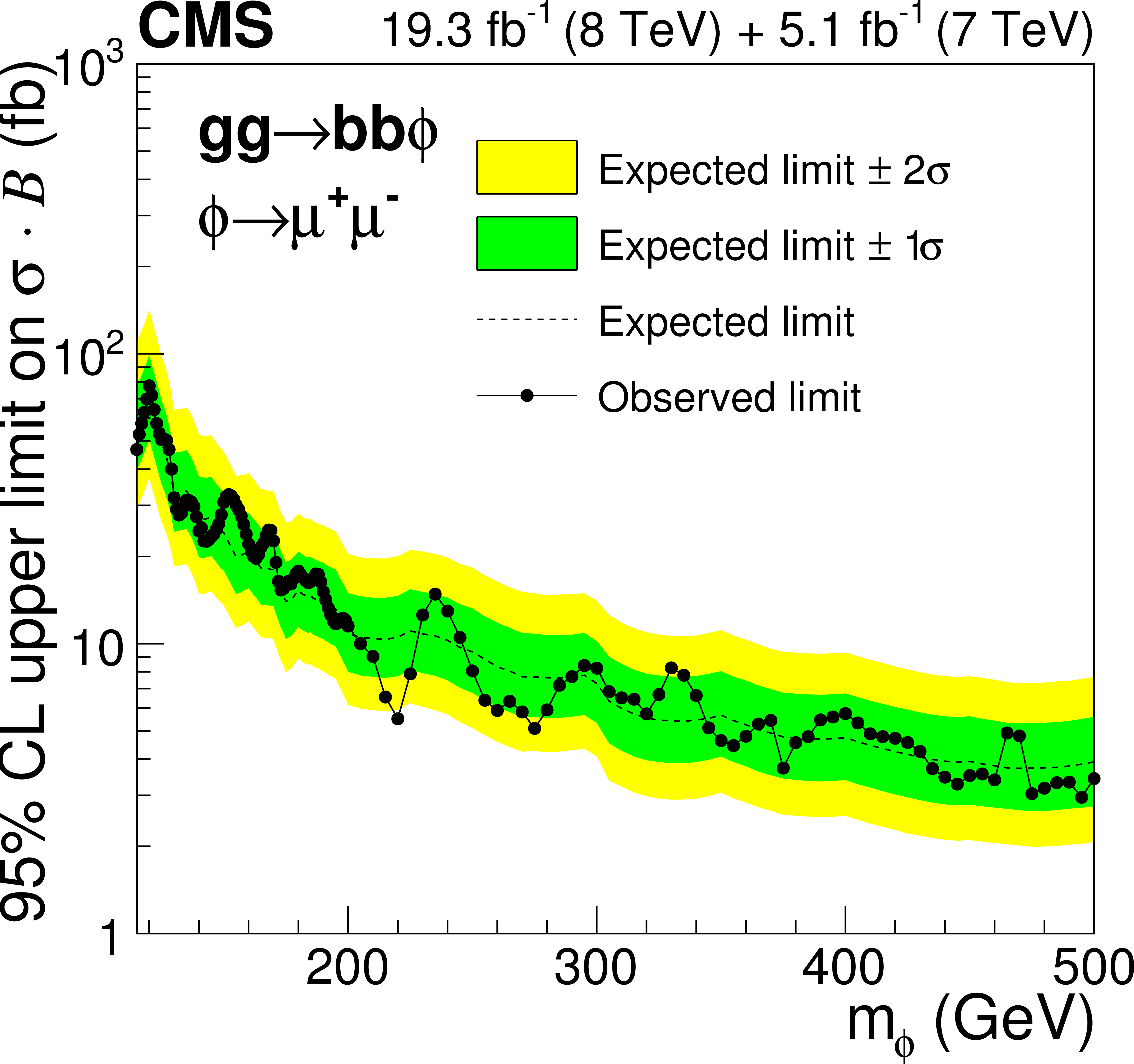
Figure 9-a:
The 95% CL limit on the product of the cross section and the decay branching fraction to two muons as a function of $m_{\phi }$, obtained from a model independent analysis of the data. The results refer to (left) b quark associated and (right) gluon fusion production, obtained using data collected at $\sqrt {s}=$ 8 TeV. |
png pdf |
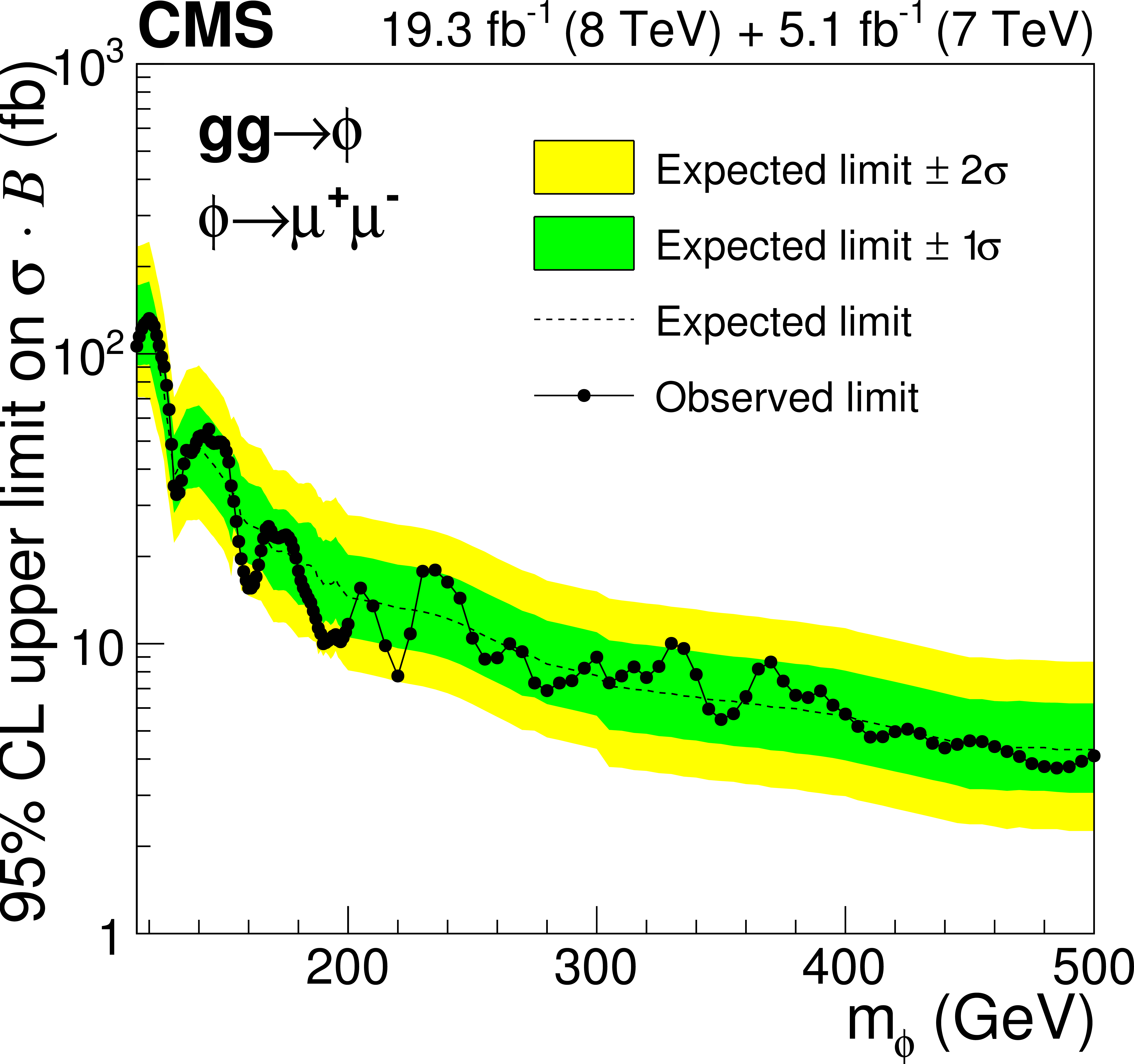
Figure 9-b:
The 95% CL limit on the product of the cross section and the decay branching fraction to two muons as a function of $m_{\phi }$, obtained from a model independent analysis of the data. The results refer to (left) b quark associated and (right) gluon fusion production, obtained using data collected at $\sqrt {s}=$ 8 TeV. |
| Tables | |
png pdf |
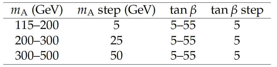
Table 1:
The $m_{ {\mathrm {A}} }$ and $\tan \beta $ values used to generate signal samples. |
png pdf |
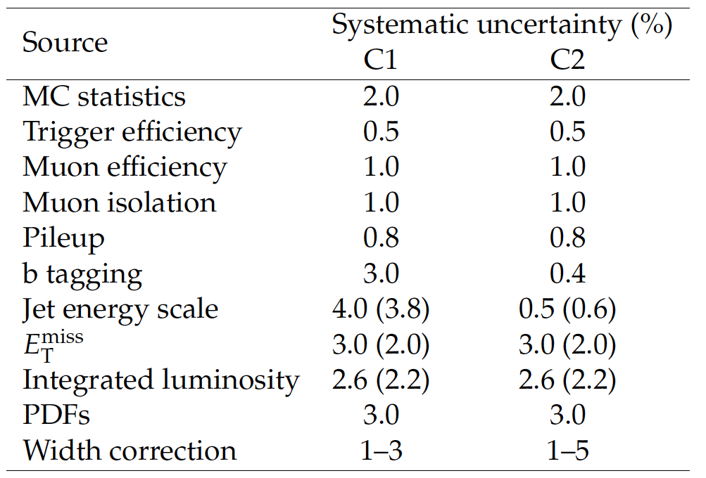
Table 2:
Sources of systematic uncertainties for C1 and C2 event categories that affect the signal efficiency at $\sqrt {s}=$ 8 TeV. They are expressed in terms of relative signal selection efficiency. When the systematic uncertainty at $\sqrt {s}=$ 7 TeV differs from $\sqrt {s}=$ 8 TeV, the corresponding value is quoted in parenthesis. |
| Summary |
| This paper presents a search for the anomalous production of events with a photon, an electron or muon, and large missing transverse momentum produced in proton-proton collisions at $\sqrt{s} = $ 8 TeV. The data are examined in bins of the photon transverse energy, the magnitude of the missing momentum, and $H_{\mathrm{T}}$, the scalar sum of jet energies. The standard model background is evaluated primarily using control samples in the data, with simulation used to evaluate backgrounds from electroweak processes. No excess of events above the standard model expectation is observed. The results of the search are interpreted as 95% confidence level upper limits on the production of new-physics events in the context of a gauge-mediated supersymmetry breaking (GMSB) model. The GMSB model is excluded for wino masses below 360 GeV. Results are also interpreted in the context of two simplified models inspired by GMSB, denoted TChiWg and T5Wg. The TChiWg model is excluded for gaugino masses below 540 GeV or, if the cross sections are scaled by the weak mixing angle, below 340 GeV. The T5Wg model with gaugino mass above 200GeV is excluded for gluino masses below 1 TeV. |
|
|
Compact Muon Solenoid LHC, CERN |
|

|

|

|

|

|