

Compact Muon Solenoid
LHC, CERN
| CMS-HIG-13-029 ; CERN-PH-EP-2014-189 | ||
| Search for the associated production of the Higgs boson with a top-quark pair | ||
| CMS Collaboration | ||
| 8 August 2014 | ||
| J. High Energy Phys. 09 (2014) 087 [Erratum] | ||
| Abstract: A search for the standard model Higgs boson produced in association with a top-quark pair ($t\bar{t}$H) is presented, using data samples corresponding to integrated luminosities of up to 5.1 fb$^{-1}$ and 19.7 fb$^{-1}$ collected in pp collisions at center-of-mass energies of 7 TeV and 8 TeV respectively. The search is based on the following signatures of the Higgs boson decay: H $\to$ hadrons, H $\to$ photons, and H $\to$ leptons. The results are characterized by an observed $t\bar{t}$H signal strength relative to the standard model cross section, $\mu$ =$\sigma/\sigma_{\mathrm{SM}}$, under the assumption that the Higgs boson decays as expected in the standard model. The best fit value is $\mu$ =2.8 $\pm$ 1.0 for a Higgs boson mass of 125.6 GeV. | ||
| Links: e-print arXiv:1408.1682 [hep-ex] (PDF) ; CDS record ; inSPIRE record ; Public twiki page ; CADI line (restricted) ; | ||
| Figures & Tables | Summary | Additional Figures | CMS Publications |
|---|
| Figures | |

png pdf |
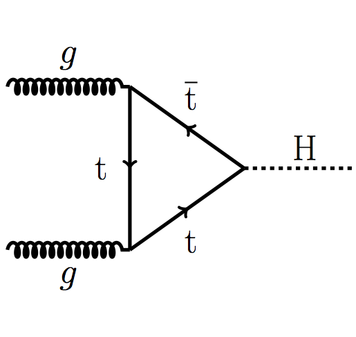
Figure 1:
Feynman diagrams showing the gluon fusion production of a Higgs boson through a top-quark loop (left), the decay of a Higgs boson to a pair of photons through a top-quark loop (center), and the production of a Higgs boson in association with a top-quark pair (right). These diagrams are representative of SM processes with sensitivity to the coupling between the top quark and the Higgs boson. |
png pdf |
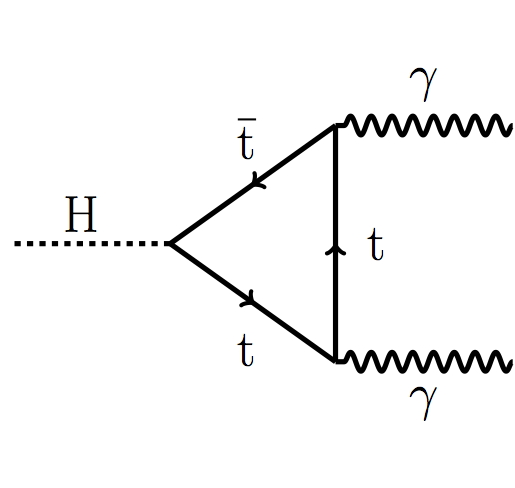
Figure 1-a:
Feynman diagrams showing the gluon fusion production of a Higgs boson through a top-quark loop (left), the decay of a Higgs boson to a pair of photons through a top-quark loop (center), and the production of a Higgs boson in association with a top-quark pair (right). These diagrams are representative of SM processes with sensitivity to the coupling between the top quark and the Higgs boson. |
png pdf |
Figure 1-b:
Feynman diagrams showing the gluon fusion production of a Higgs boson through a top-quark loop (left), the decay of a Higgs boson to a pair of photons through a top-quark loop (center), and the production of a Higgs boson in association with a top-quark pair (right). These diagrams are representative of SM processes with sensitivity to the coupling between the top quark and the Higgs boson. |
png pdf |
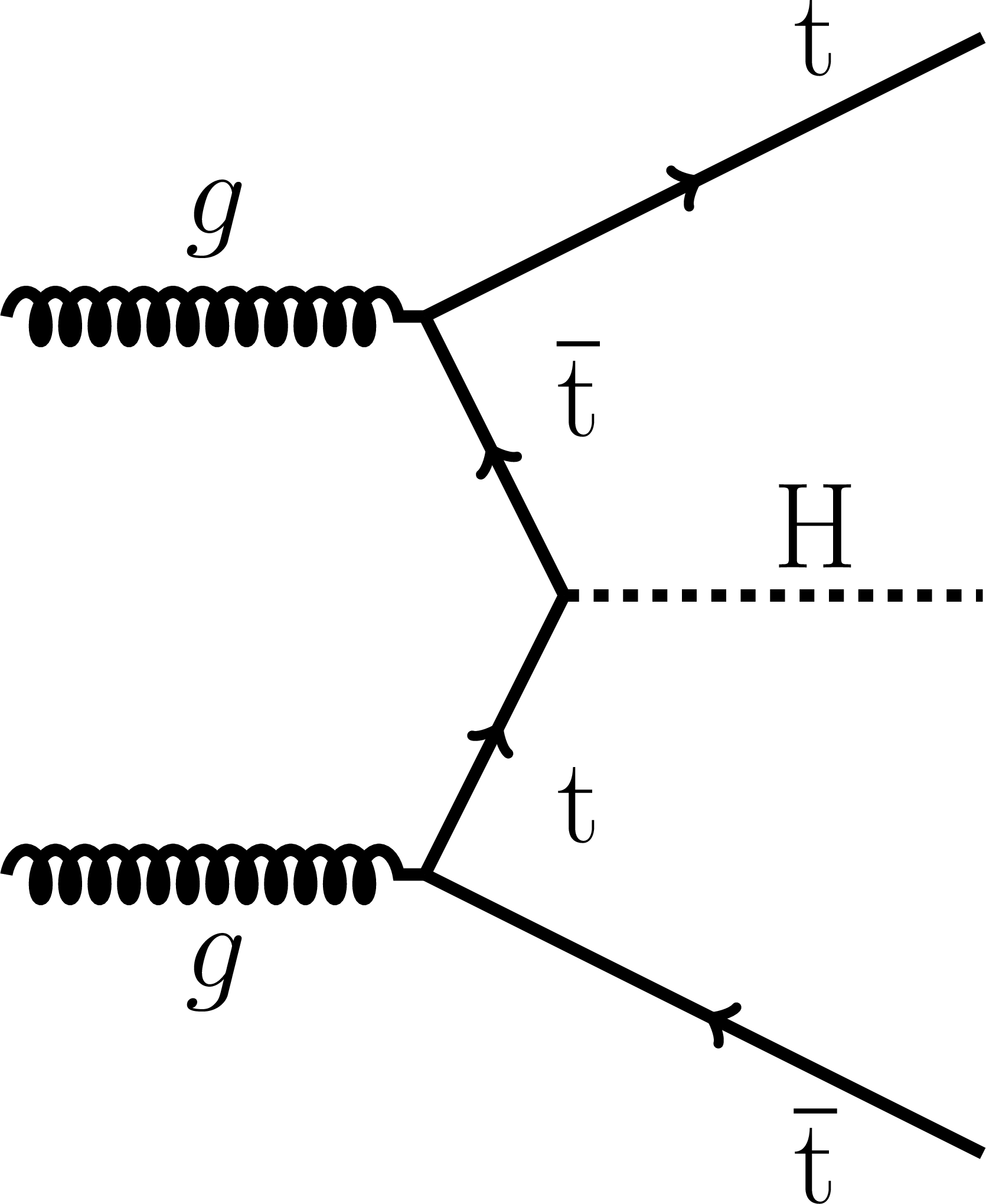
Figure 1-c:
Feynman diagrams showing the gluon fusion production of a Higgs boson through a top-quark loop (left), the decay of a Higgs boson to a pair of photons through a top-quark loop (center), and the production of a Higgs boson in association with a top-quark pair (right). These diagrams are representative of SM processes with sensitivity to the coupling between the top quark and the Higgs boson. |
png pdf |
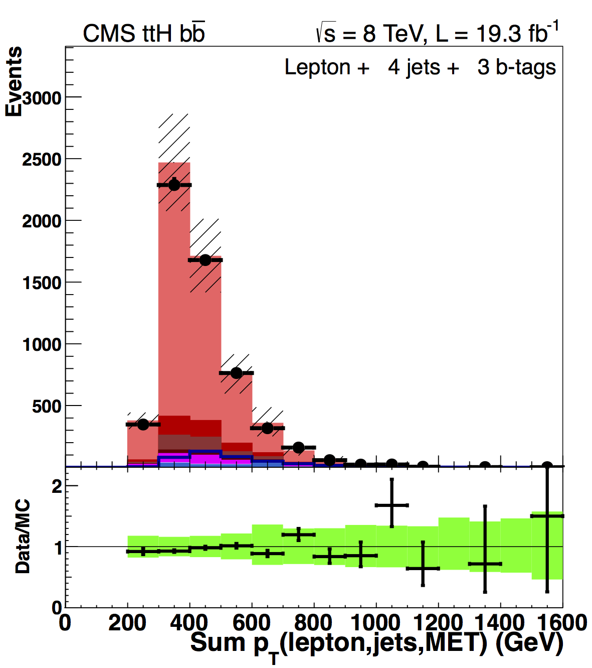
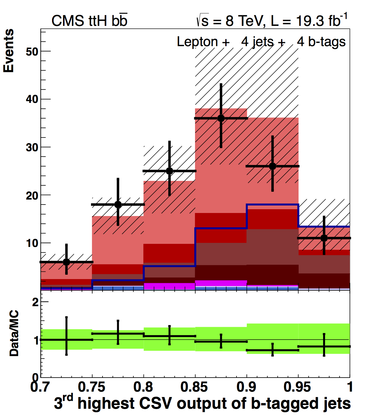
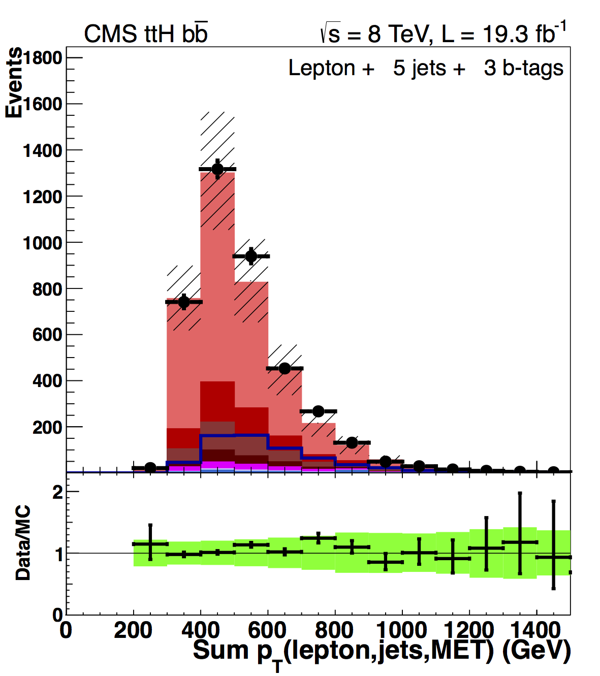
Figure 2:
Input variables that give the best signal-background separation for each of the lepton+jets categories used in the analysis at $\sqrt {s} = 8 TeV $. The top, middle, and bottom rows show the events with 4, 5, and $\ge $6 jets, respectively, while the left, middle, and right columns are events with 2, 3, and $\ge $4 b-tags, respectively. More details regarding these plots are found in the text. |
png pdf |
Figure 2-a:
Input variables that give the best signal-background separation for each of the lepton+jets categories used in the analysis at $\sqrt {s} = 8 TeV $. The top, middle, and bottom rows show the events with 4, 5, and $\ge $6 jets, respectively, while the left, middle, and right columns are events with 2, 3, and $\ge $4 b-tags, respectively. More details regarding these plots are found in the text. |
png pdf |
Figure 2-b:
Input variables that give the best signal-background separation for each of the lepton+jets categories used in the analysis at $\sqrt {s} = 8 TeV $. The top, middle, and bottom rows show the events with 4, 5, and $\ge $6 jets, respectively, while the left, middle, and right columns are events with 2, 3, and $\ge $4 b-tags, respectively. More details regarding these plots are found in the text. |
png pdf |
Figure 2-c:
Input variables that give the best signal-background separation for each of the lepton+jets categories used in the analysis at $\sqrt {s} = 8 TeV $. The top, middle, and bottom rows show the events with 4, 5, and $\ge $6 jets, respectively, while the left, middle, and right columns are events with 2, 3, and $\ge $4 b-tags, respectively. More details regarding these plots are found in the text. |
png pdf |
Figure 2-d:
Input variables that give the best signal-background separation for each of the lepton+jets categories used in the analysis at $\sqrt {s} = 8 TeV $. The top, middle, and bottom rows show the events with 4, 5, and $\ge $6 jets, respectively, while the left, middle, and right columns are events with 2, 3, and $\ge $4 b-tags, respectively. More details regarding these plots are found in the text. |

png pdf |
Figure 2-e:
Input variables that give the best signal-background separation for each of the lepton+jets categories used in the analysis at $\sqrt {s} = 8 TeV $. The top, middle, and bottom rows show the events with 4, 5, and $\ge $6 jets, respectively, while the left, middle, and right columns are events with 2, 3, and $\ge $4 b-tags, respectively. More details regarding these plots are found in the text. |

png pdf |
Figure 2-f:
Input variables that give the best signal-background separation for each of the lepton+jets categories used in the analysis at $\sqrt {s} = 8 TeV $. The top, middle, and bottom rows show the events with 4, 5, and $\ge $6 jets, respectively, while the left, middle, and right columns are events with 2, 3, and $\ge $4 b-tags, respectively. More details regarding these plots are found in the text. |
png pdf |
Figure 2-g:
Input variables that give the best signal-background separation for each of the lepton+jets categories used in the analysis at $\sqrt {s} = 8 TeV $. The top, middle, and bottom rows show the events with 4, 5, and $\ge $6 jets, respectively, while the left, middle, and right columns are events with 2, 3, and $\ge $4 b-tags, respectively. More details regarding these plots are found in the text. |

png pdf |
Figure 2-h:
Input variables that give the best signal-background separation for each of the lepton+jets categories used in the analysis at $\sqrt {s} = 8 TeV $. The top, middle, and bottom rows show the events with 4, 5, and $\ge $6 jets, respectively, while the left, middle, and right columns are events with 2, 3, and $\ge $4 b-tags, respectively. More details regarding these plots are found in the text. |
png pdf |
Figure 3-a:
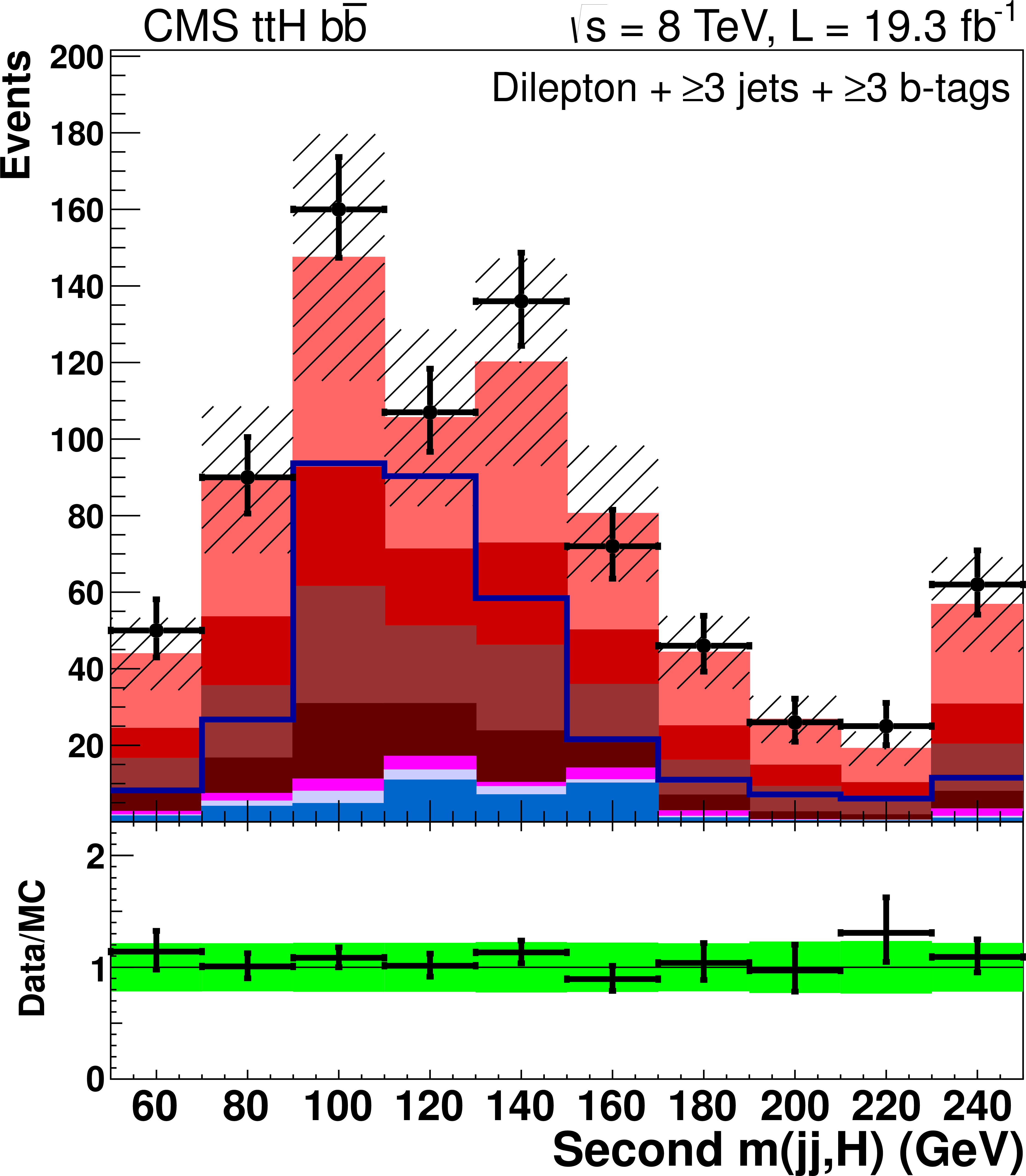
Input variables that give the best signal-background separation for each of the dilepton categories used in the analysis at $\sqrt {s} = 8 TeV $. The left, middle, and right panels show the events with 3 jets and 2 b-tags, $\ge $4 jets and 2 b-tags, and $\ge $3 b-tags, respectively. More details regarding these plots are found in the text. |
png pdf |
Figure 3-b:
Input variables that give the best signal-background separation for each of the dilepton categories used in the analysis at $\sqrt {s} = 8 TeV $. The left, middle, and right panels show the events with 3 jets and 2 b-tags, $\ge $4 jets and 2 b-tags, and $\ge $3 b-tags, respectively. More details regarding these plots are found in the text. |
png pdf |
Figure 3-c:
Input variables that give the best signal-background separation for each of the dilepton categories used in the analysis at $\sqrt {s} = 8 TeV $. The left, middle, and right panels show the events with 3 jets and 2 b-tags, $\ge $4 jets and 2 b-tags, and $\ge $3 b-tags, respectively. More details regarding these plots are found in the text. |
png pdf |
Figure 3-d:
Input variables that give the best signal-background separation for each of the dilepton categories used in the analysis at $\sqrt {s} = 8 TeV $. The left, middle, and right panels show the events with 3 jets and 2 b-tags, $\ge $4 jets and 2 b-tags, and $\ge $3 b-tags, respectively. More details regarding these plots are found in the text. |

png pdf |
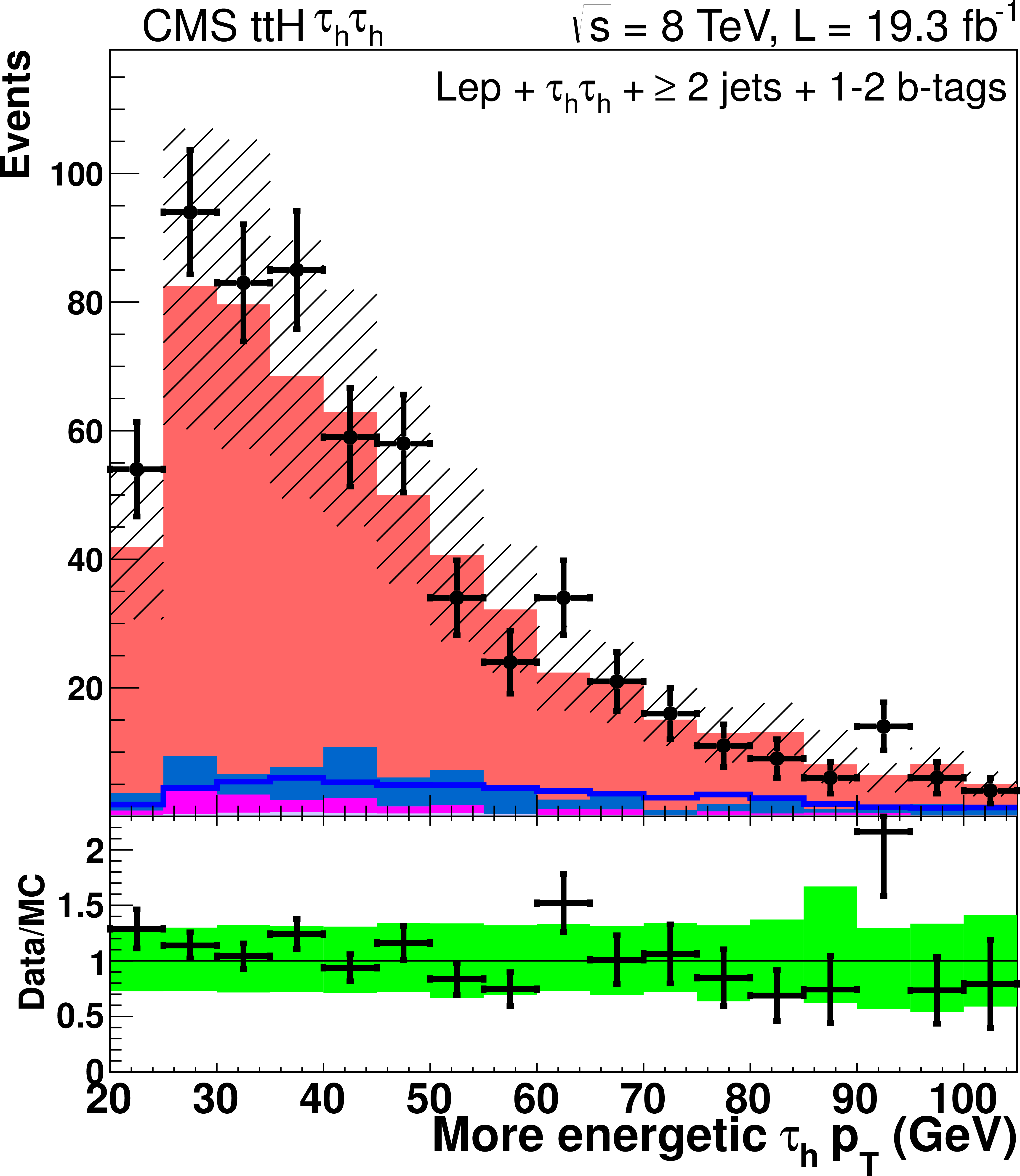
Figure 4-a:
Examples of input variables that give the best signal-background separation in the analysis of the $ {\tau _\mathrm {h}} $ channels at $\sqrt {s} = 8 TeV $. The left plot shows the $ {p_{\mathrm {T}}} $ of the more energetic $ {\tau _\mathrm {h}} $, while the right plot displays $M_\mathrm {vis}$, the mass of the visible $ {\tau _\mathrm {h}} $ decay products. Events of all categories are shown. More details regarding these plots are found in the text. |
png pdf |
Figure 4-b:
Examples of input variables that give the best signal-background separation in the analysis of the $ {\tau _\mathrm {h}} $ channels at $\sqrt {s} = 8 TeV $. The left plot shows the $ {p_{\mathrm {T}}} $ of the more energetic $ {\tau _\mathrm {h}} $, while the right plot displays $M_\mathrm {vis}$, the mass of the visible $ {\tau _\mathrm {h}} $ decay products. Events of all categories are shown. More details regarding these plots are found in the text. |
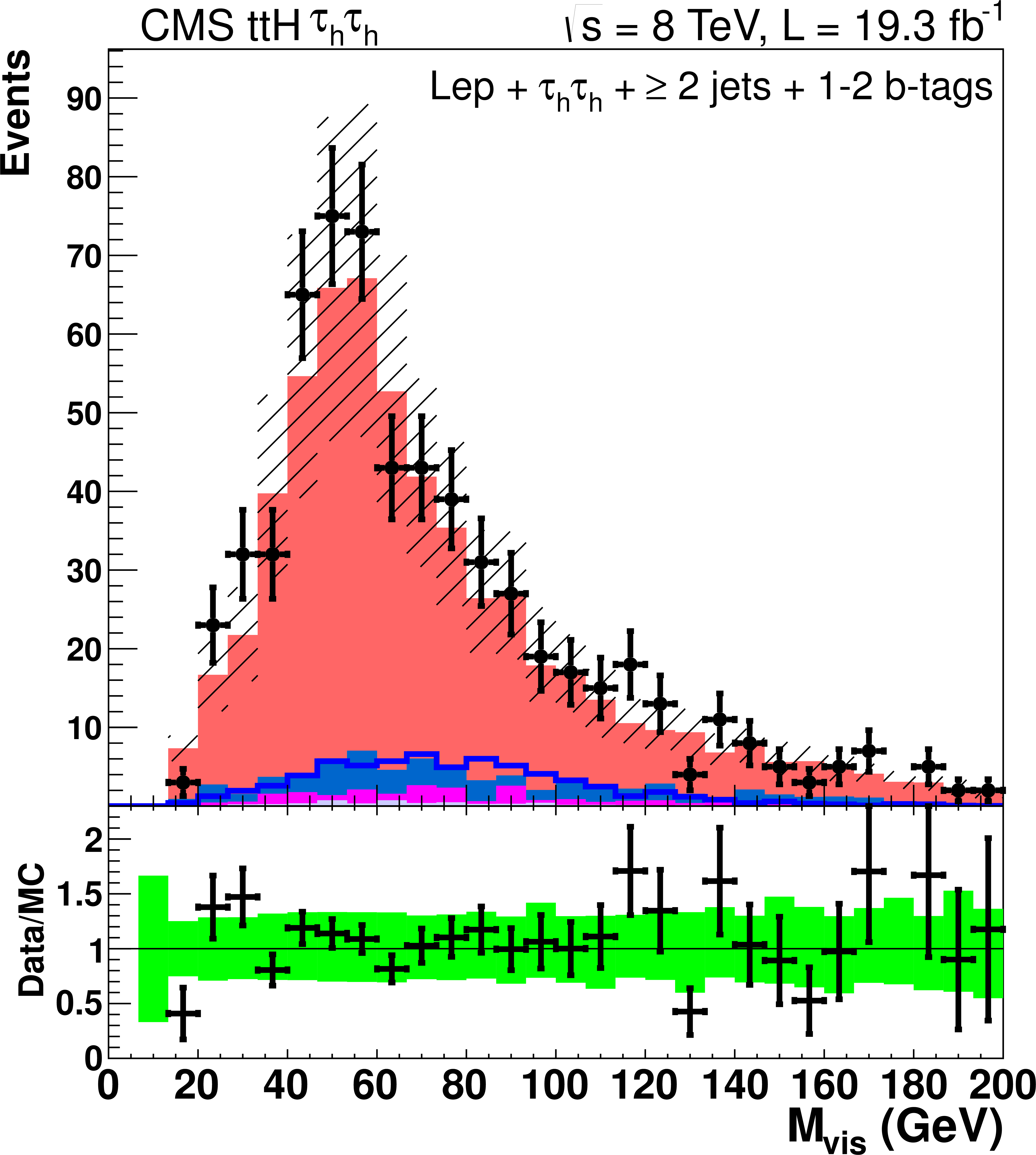
png pdf |
Figure 4-c:
Examples of input variables that give the best signal-background separation in the analysis of the $ {\tau _\mathrm {h}} $ channels at $\sqrt {s} = 8 TeV $. The left plot shows the $ {p_{\mathrm {T}}} $ of the more energetic $ {\tau _\mathrm {h}} $, while the right plot displays $M_\mathrm {vis}$, the mass of the visible $ {\tau _\mathrm {h}} $ decay products. Events of all categories are shown. More details regarding these plots are found in the text. |
png pdf |
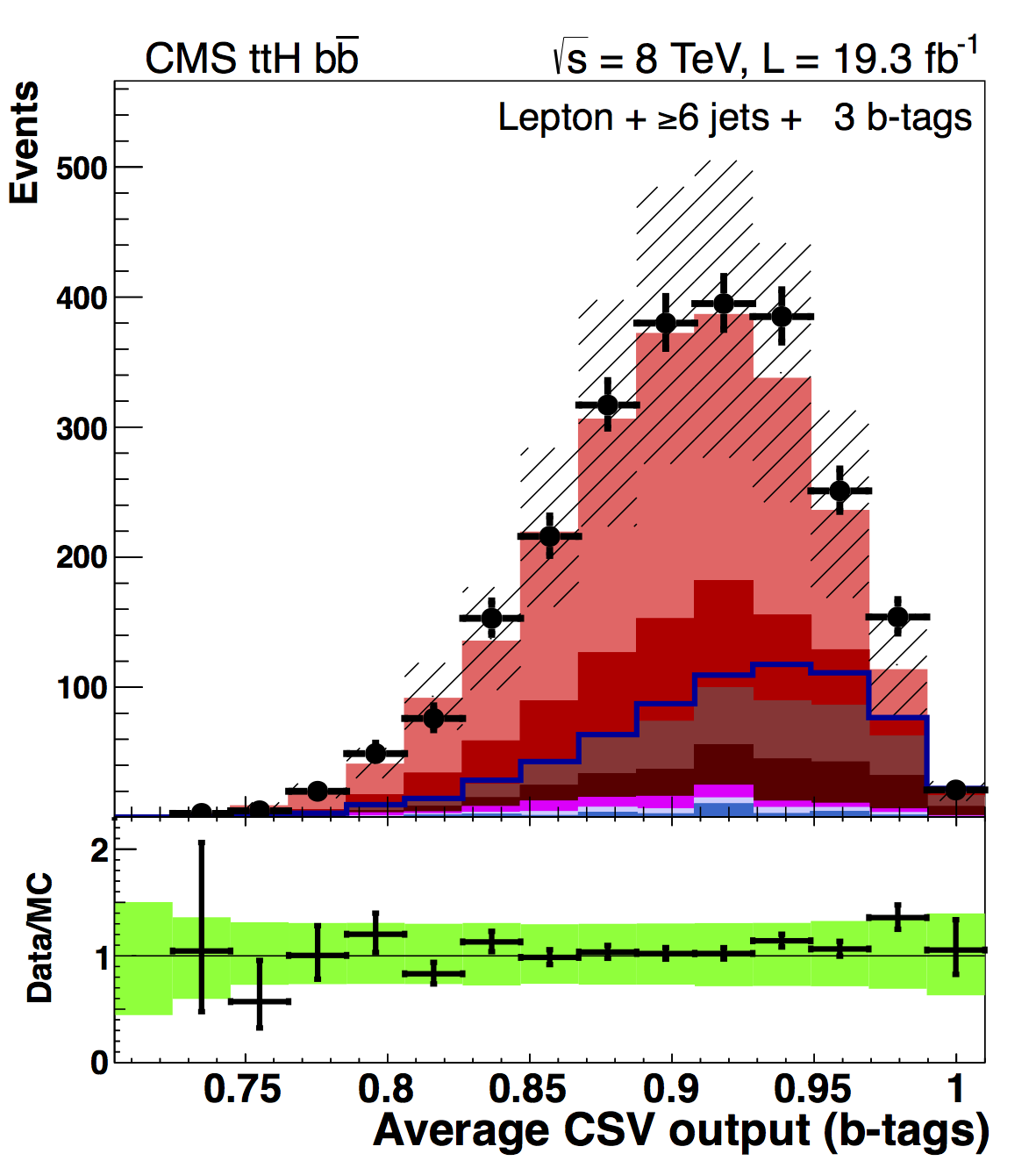
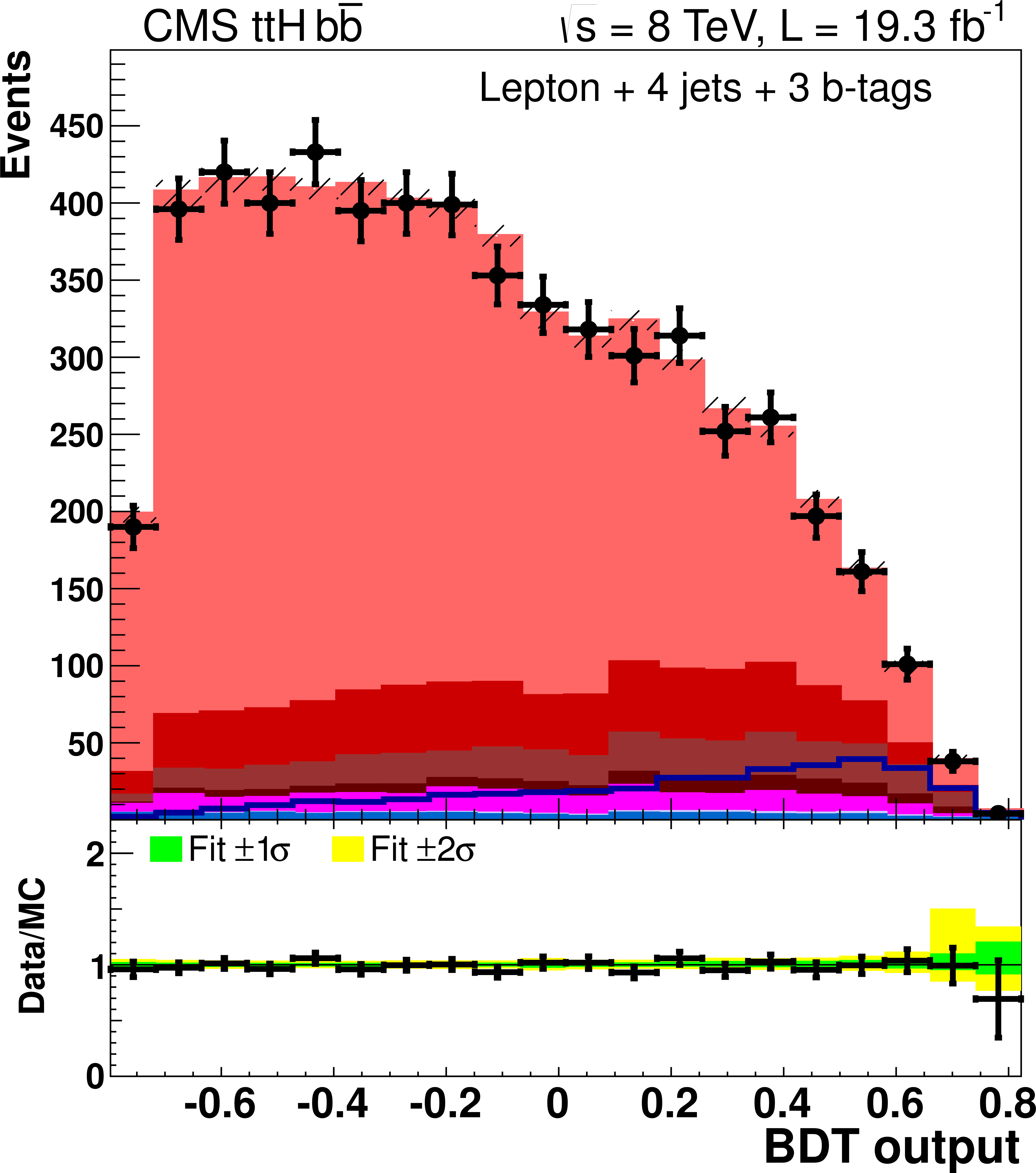
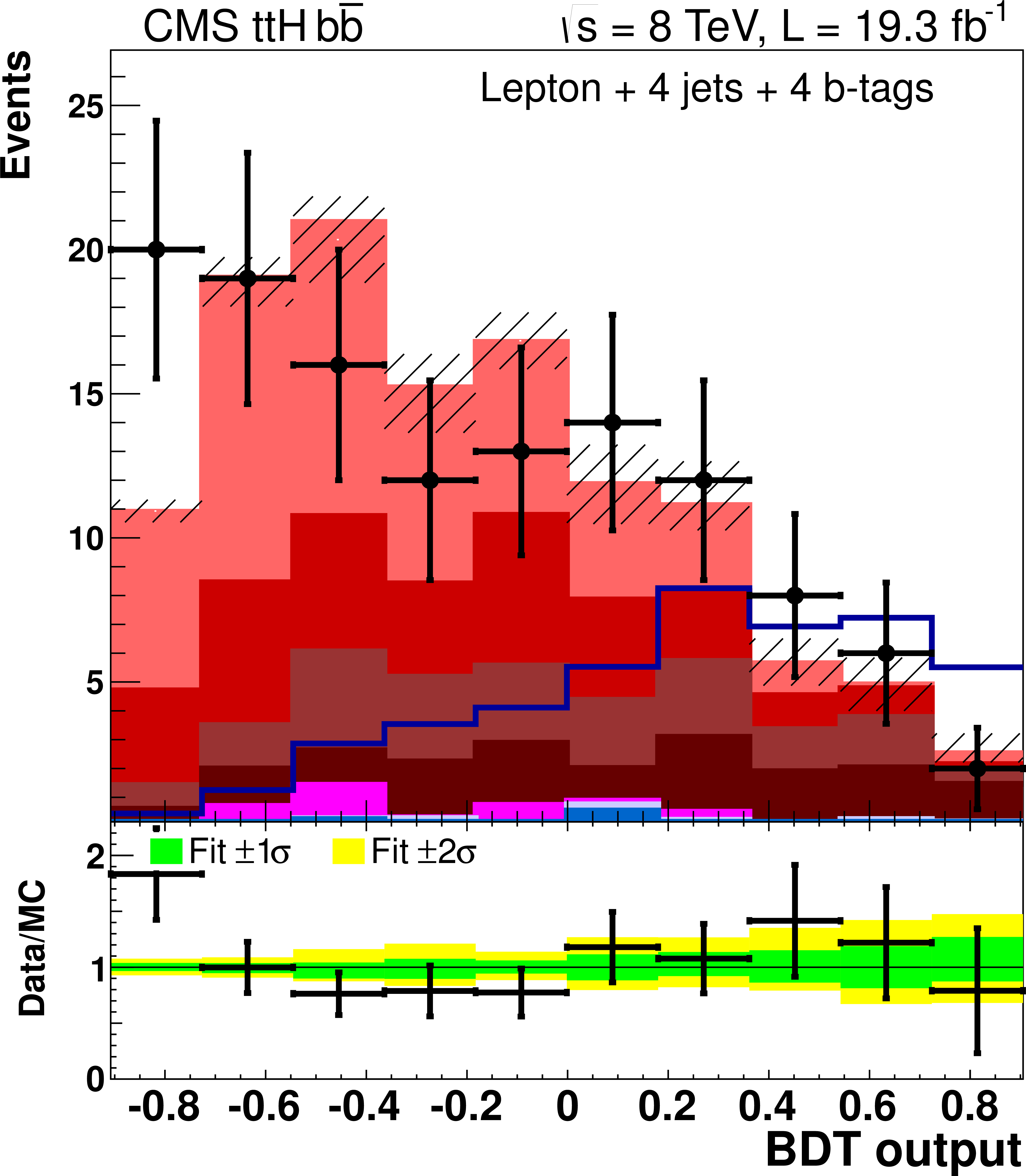
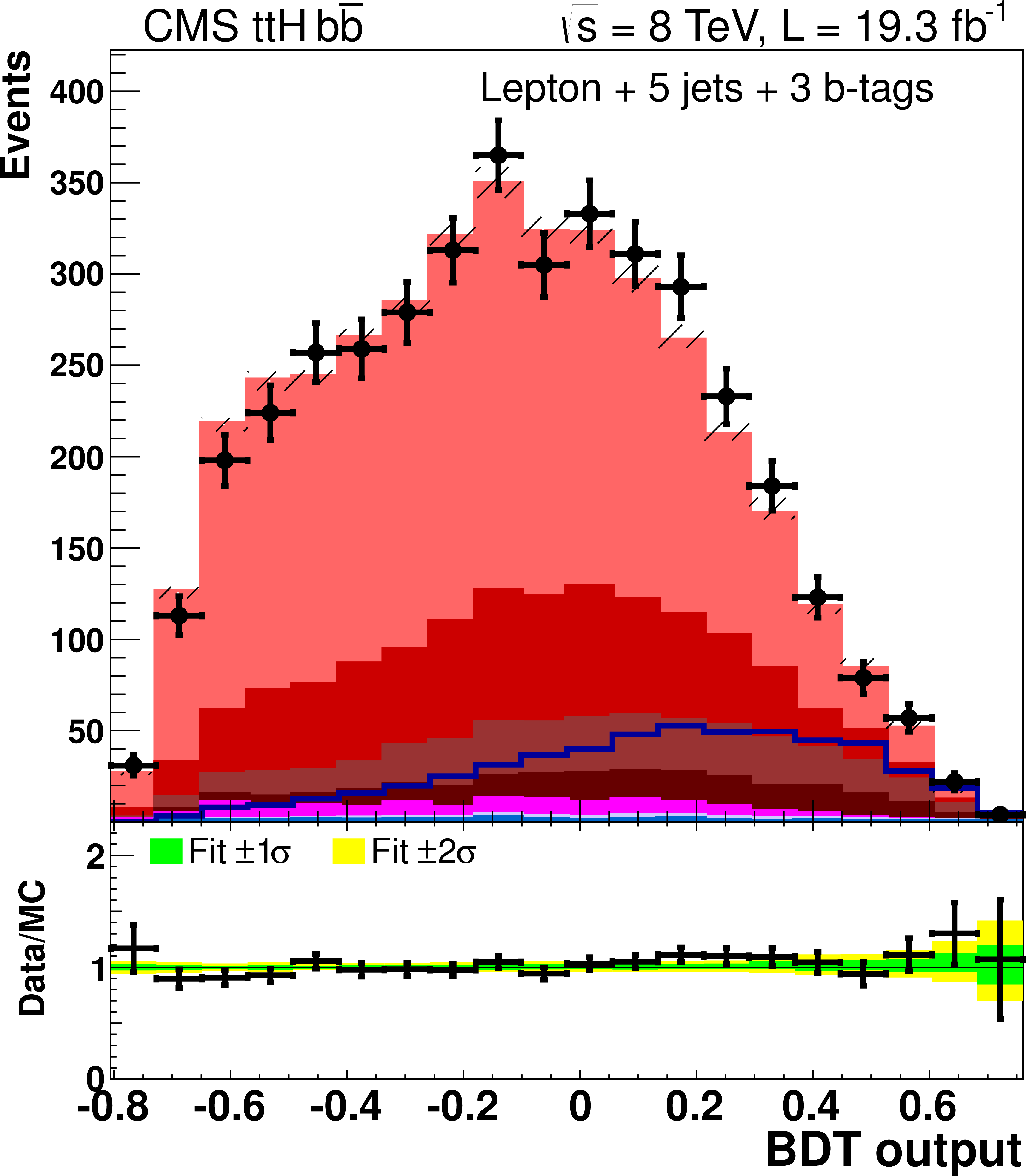
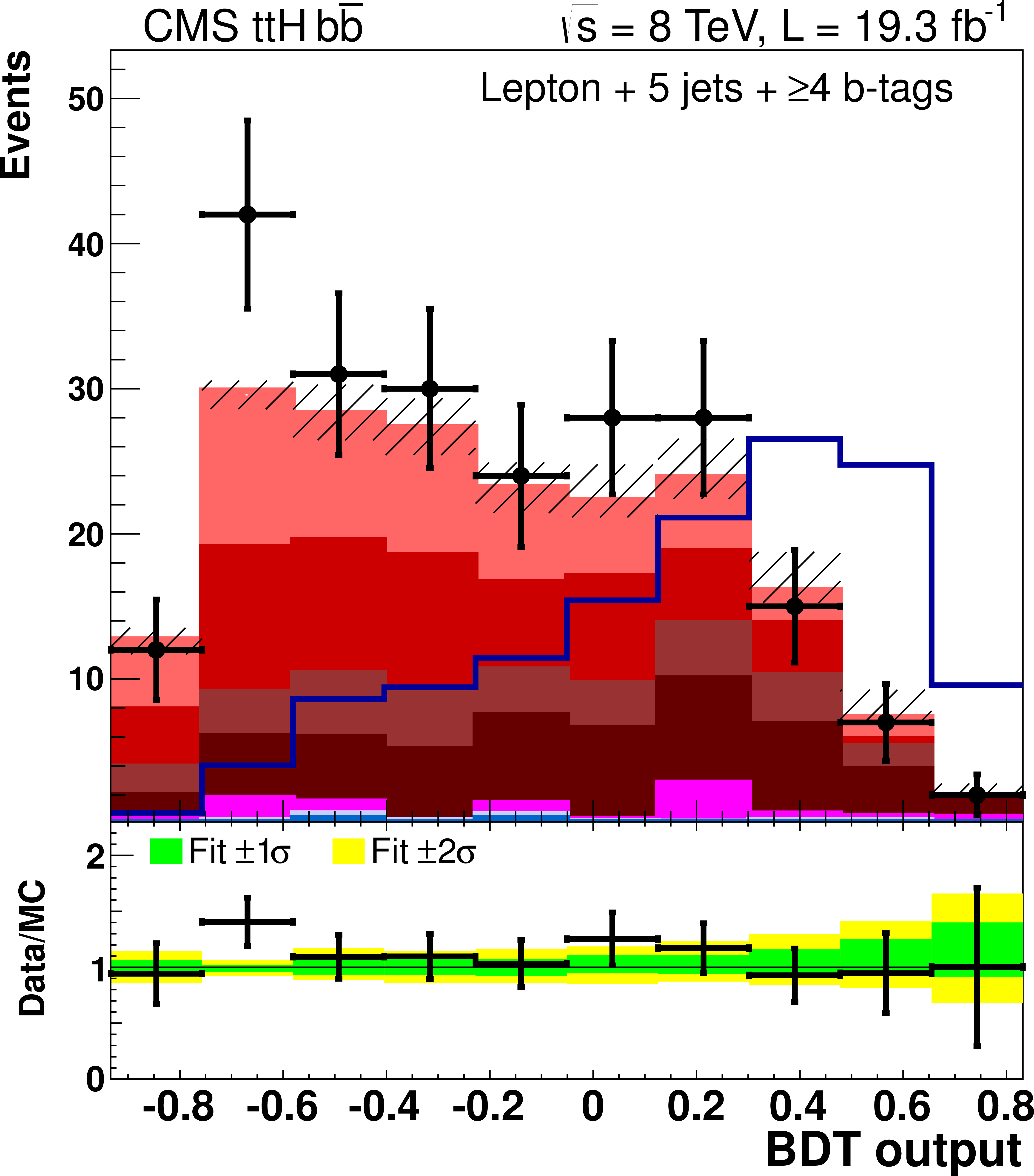
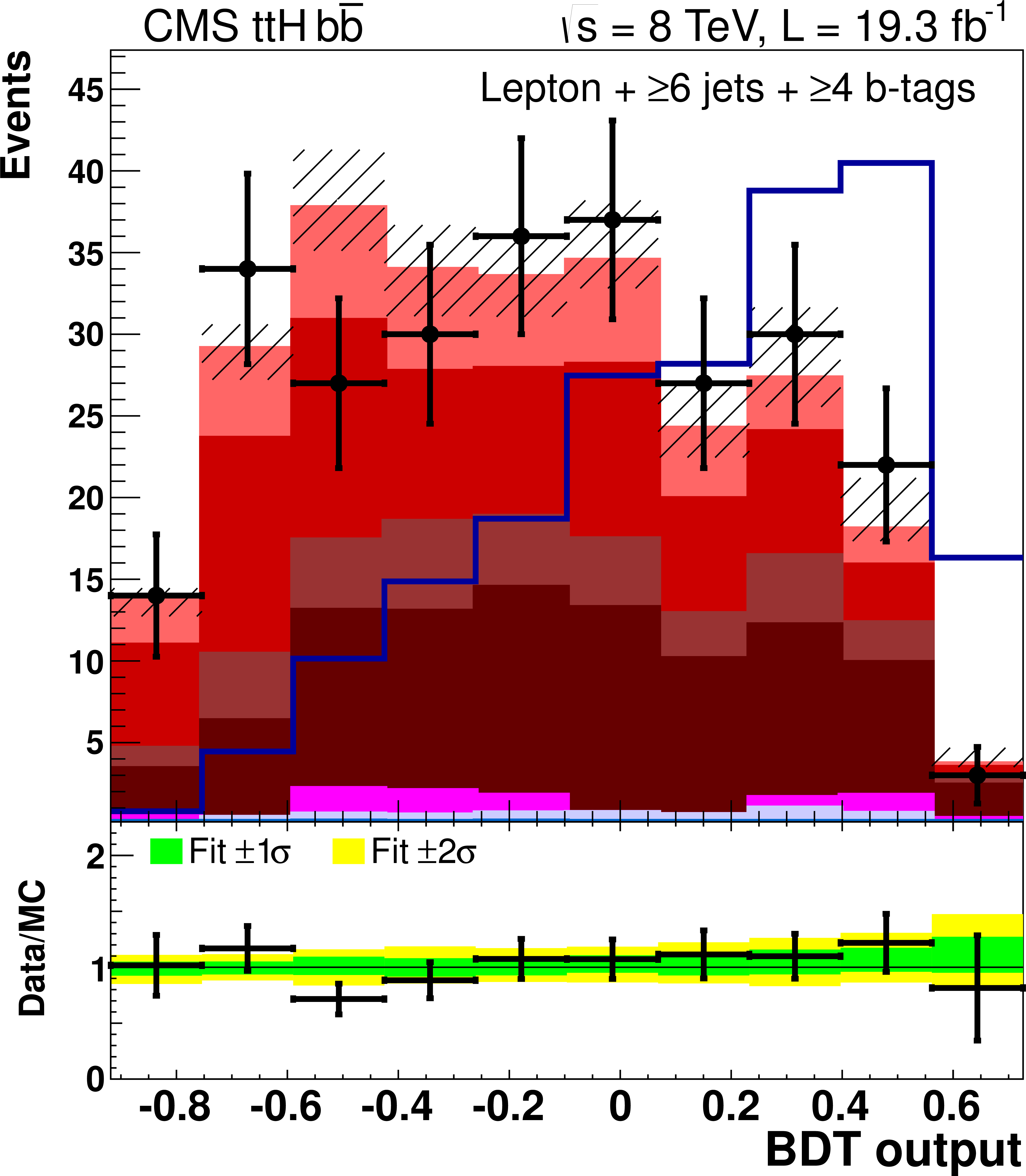
Figure 5-a:
Final BDT output for lepton+jets events. The top, middle and, bottom rows are events with 4, 5, and $\ge $6 jets, respectively, while the left, middle, and right columns are events with 2, 3, and $\ge $4 b-tags, respectively. Details regarding signal and background normalizations are described in the text. |
png pdf |
Figure 5-b:
Final BDT output for lepton+jets events. The top, middle and, bottom rows are events with 4, 5, and $\ge $6 jets, respectively, while the left, middle, and right columns are events with 2, 3, and $\ge $4 b-tags, respectively. Details regarding signal and background normalizations are described in the text. |
png pdf |
Figure 5-c:
Final BDT output for lepton+jets events. The top, middle and, bottom rows are events with 4, 5, and $\ge $6 jets, respectively, while the left, middle, and right columns are events with 2, 3, and $\ge $4 b-tags, respectively. Details regarding signal and background normalizations are described in the text. |
png pdf |
Figure 5-d:
Final BDT output for lepton+jets events. The top, middle and, bottom rows are events with 4, 5, and $\ge $6 jets, respectively, while the left, middle, and right columns are events with 2, 3, and $\ge $4 b-tags, respectively. Details regarding signal and background normalizations are described in the text. |
png pdf |
Figure 5-e:
Final BDT output for lepton+jets events. The top, middle and, bottom rows are events with 4, 5, and $\ge $6 jets, respectively, while the left, middle, and right columns are events with 2, 3, and $\ge $4 b-tags, respectively. Details regarding signal and background normalizations are described in the text. |

png pdf |
Figure 5-f:
Final BDT output for lepton+jets events. The top, middle and, bottom rows are events with 4, 5, and $\ge $6 jets, respectively, while the left, middle, and right columns are events with 2, 3, and $\ge $4 b-tags, respectively. Details regarding signal and background normalizations are described in the text. |

png pdf |
Figure 5-g:
Final BDT output for lepton+jets events. The top, middle and, bottom rows are events with 4, 5, and $\ge $6 jets, respectively, while the left, middle, and right columns are events with 2, 3, and $\ge $4 b-tags, respectively. Details regarding signal and background normalizations are described in the text. |
png pdf |
Figure 5-h:
Final BDT output for lepton+jets events. The top, middle and, bottom rows are events with 4, 5, and $\ge $6 jets, respectively, while the left, middle, and right columns are events with 2, 3, and $\ge $4 b-tags, respectively. Details regarding signal and background normalizations are described in the text. |
png pdf |
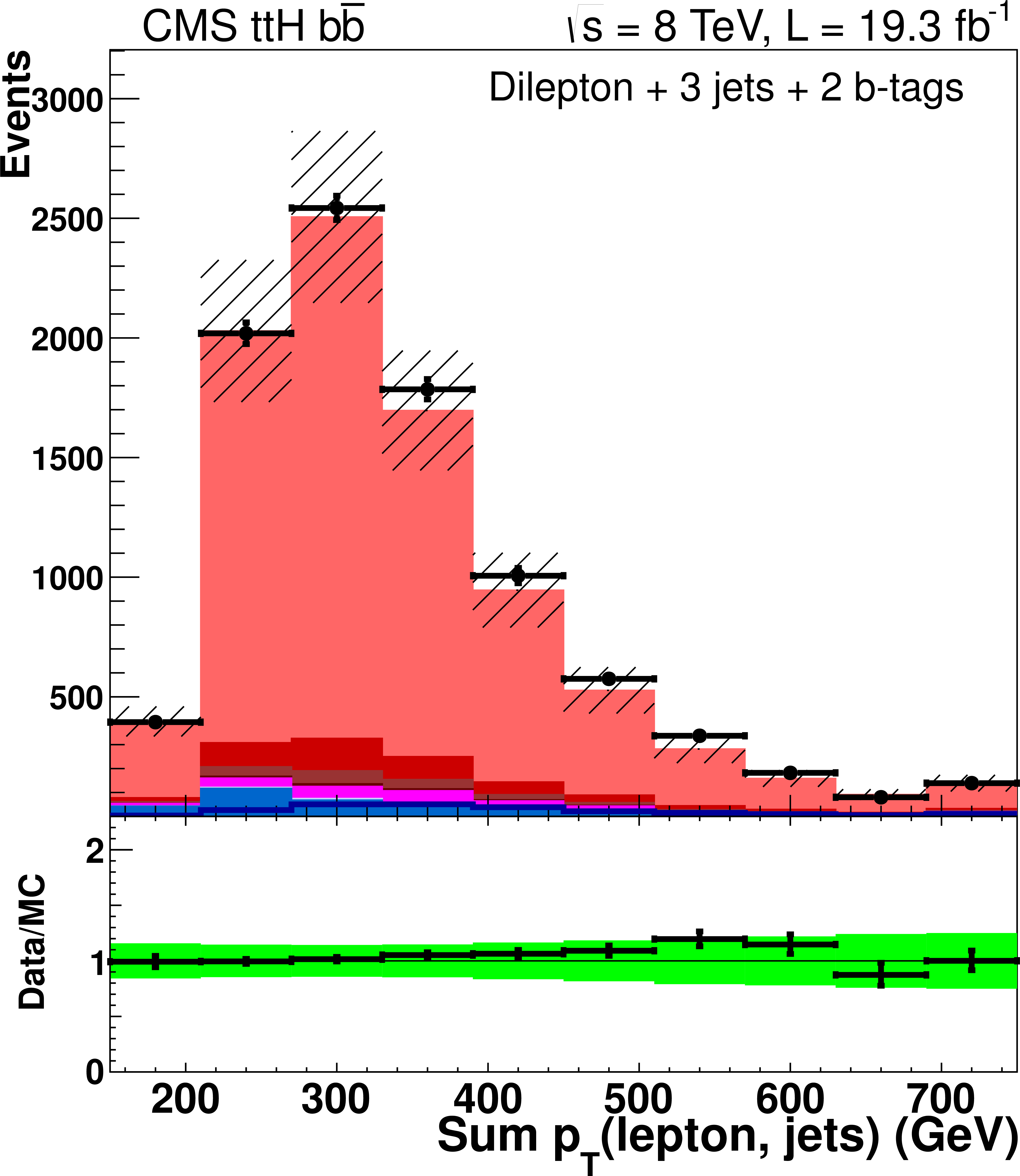
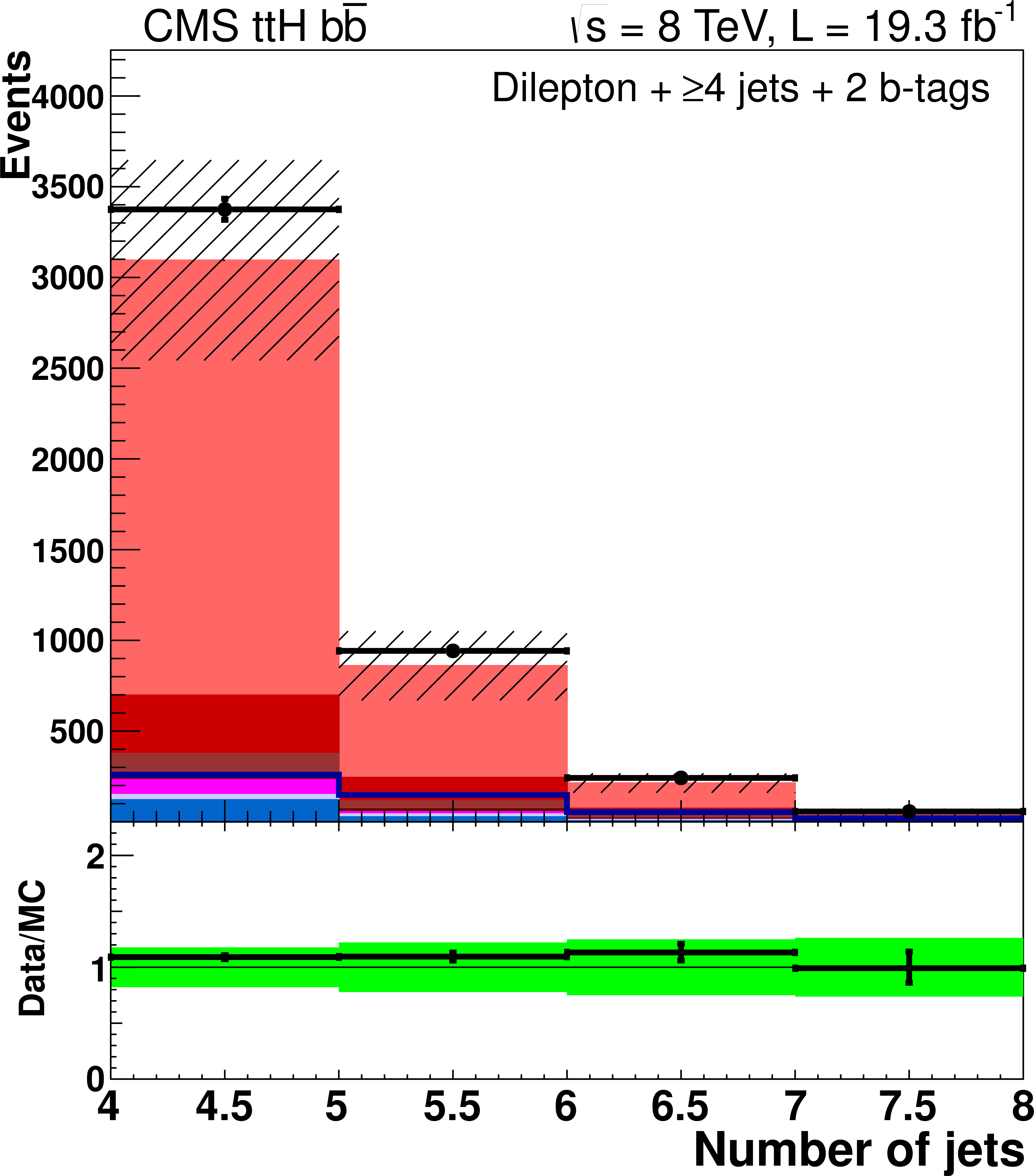
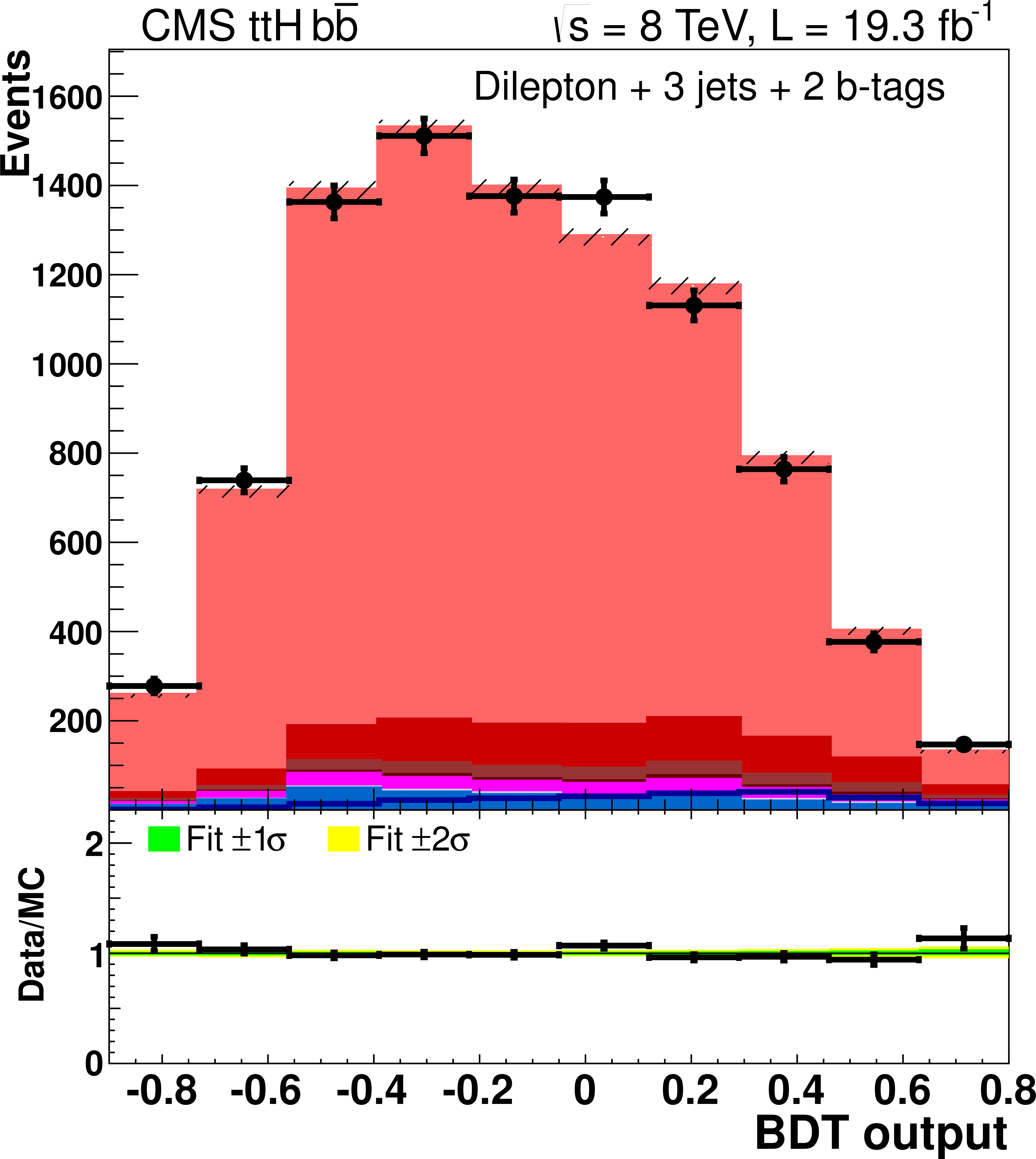
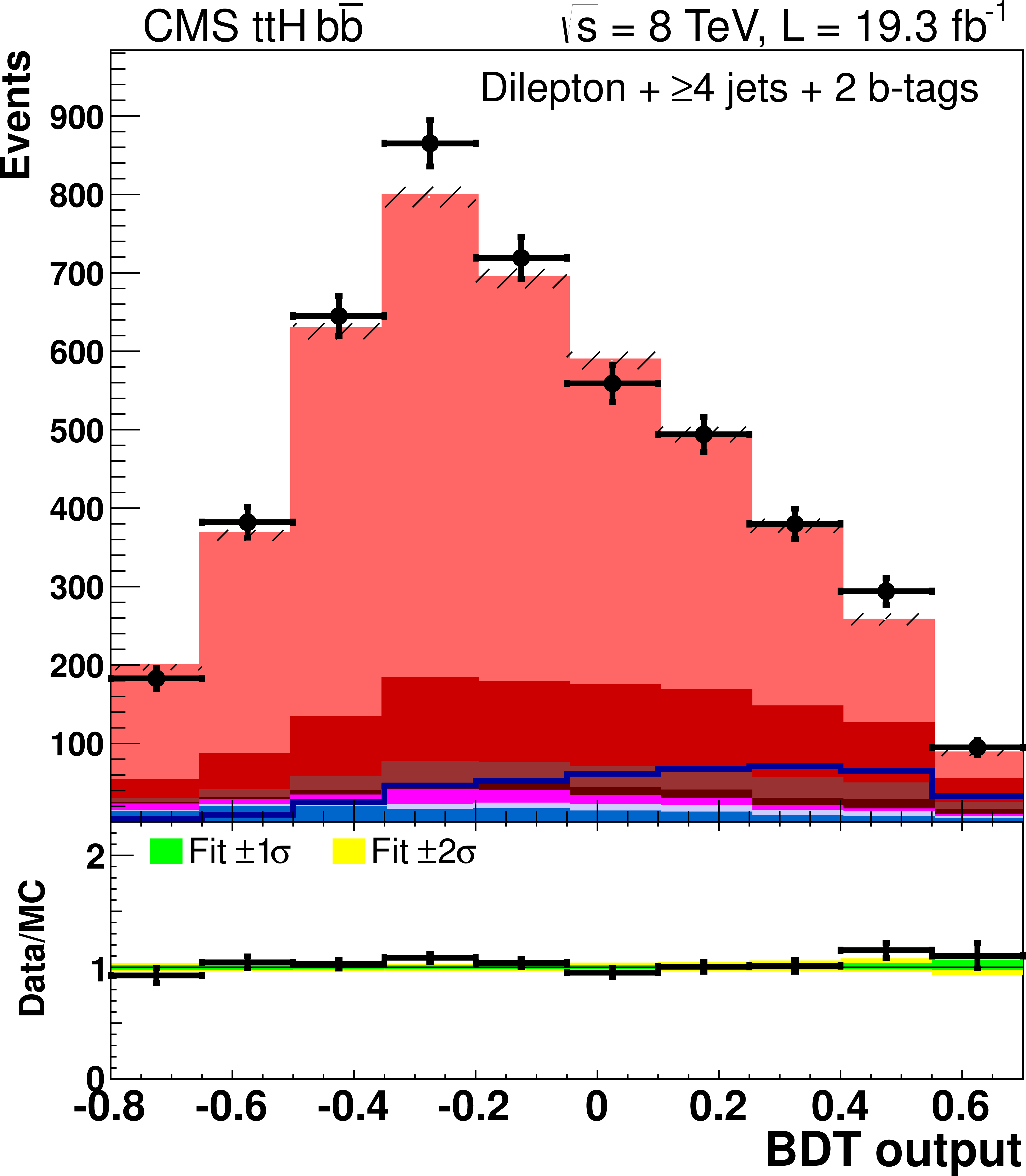
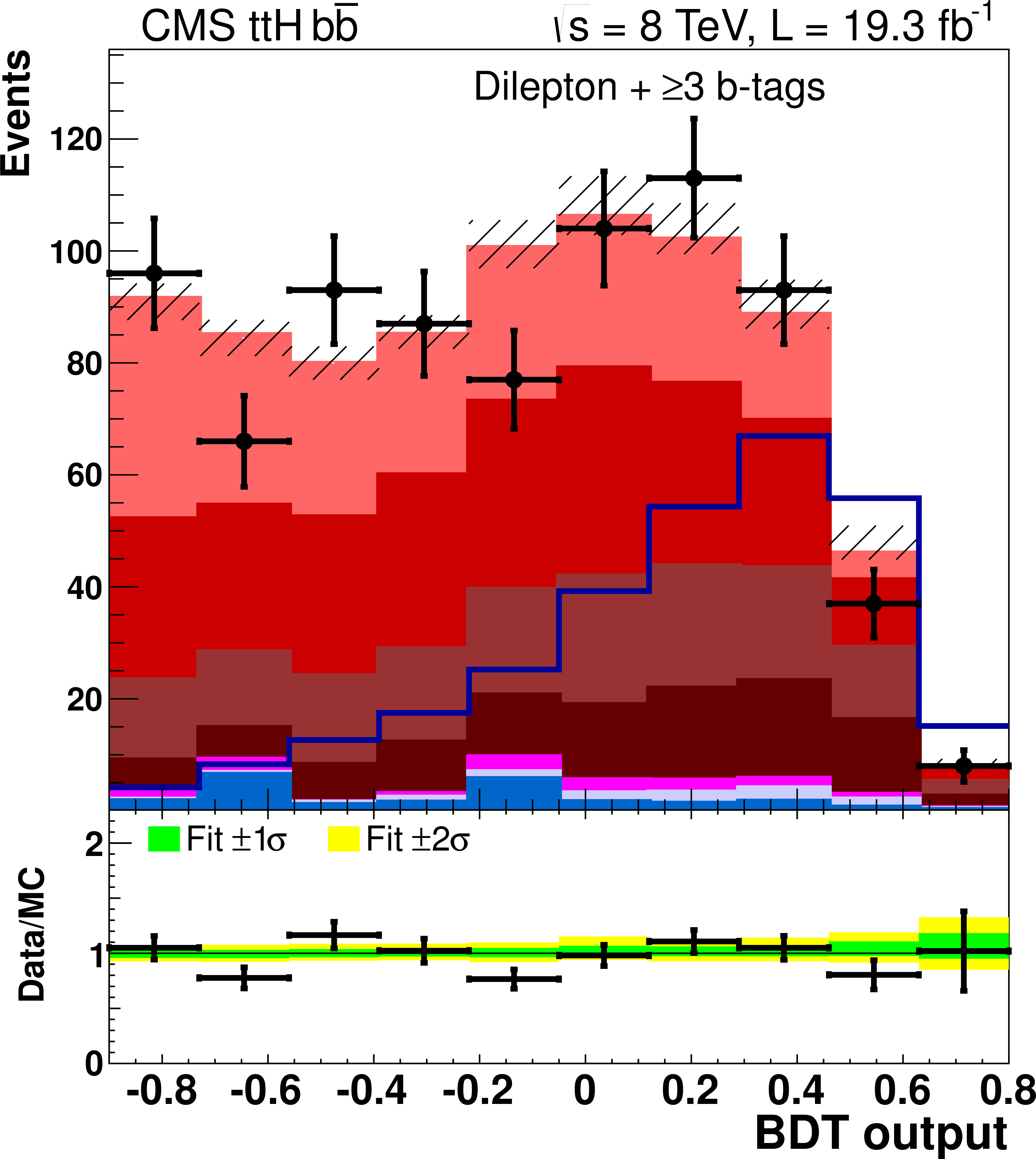
Figure 6-a:
Final BDT output for dilepton events. The upper left, upper right, and lower left plots are events with 3 jets + 2 b-tags, $\ge $4 jets + 2 b-tags, and $\ge $3 b-tags, respectively. Details regarding signal and background normalizations are described in the text. |
png pdf |
Figure 6-b:
Final BDT output for dilepton events. The upper left, upper right, and lower left plots are events with 3 jets + 2 b-tags, $\ge $4 jets + 2 b-tags, and $\ge $3 b-tags, respectively. Details regarding signal and background normalizations are described in the text. |
png pdf |
Figure 6-c:
Final BDT output for dilepton events. The upper left, upper right, and lower left plots are events with 3 jets + 2 b-tags, $\ge $4 jets + 2 b-tags, and $\ge $3 b-tags, respectively. Details regarding signal and background normalizations are described in the text. |

png pdf |
Figure 6-d:
Final BDT output for dilepton events. The upper left, upper right, and lower left plots are events with 3 jets + 2 b-tags, $\ge $4 jets + 2 b-tags, and $\ge $3 b-tags, respectively. Details regarding signal and background normalizations are described in the text. |

png pdf |
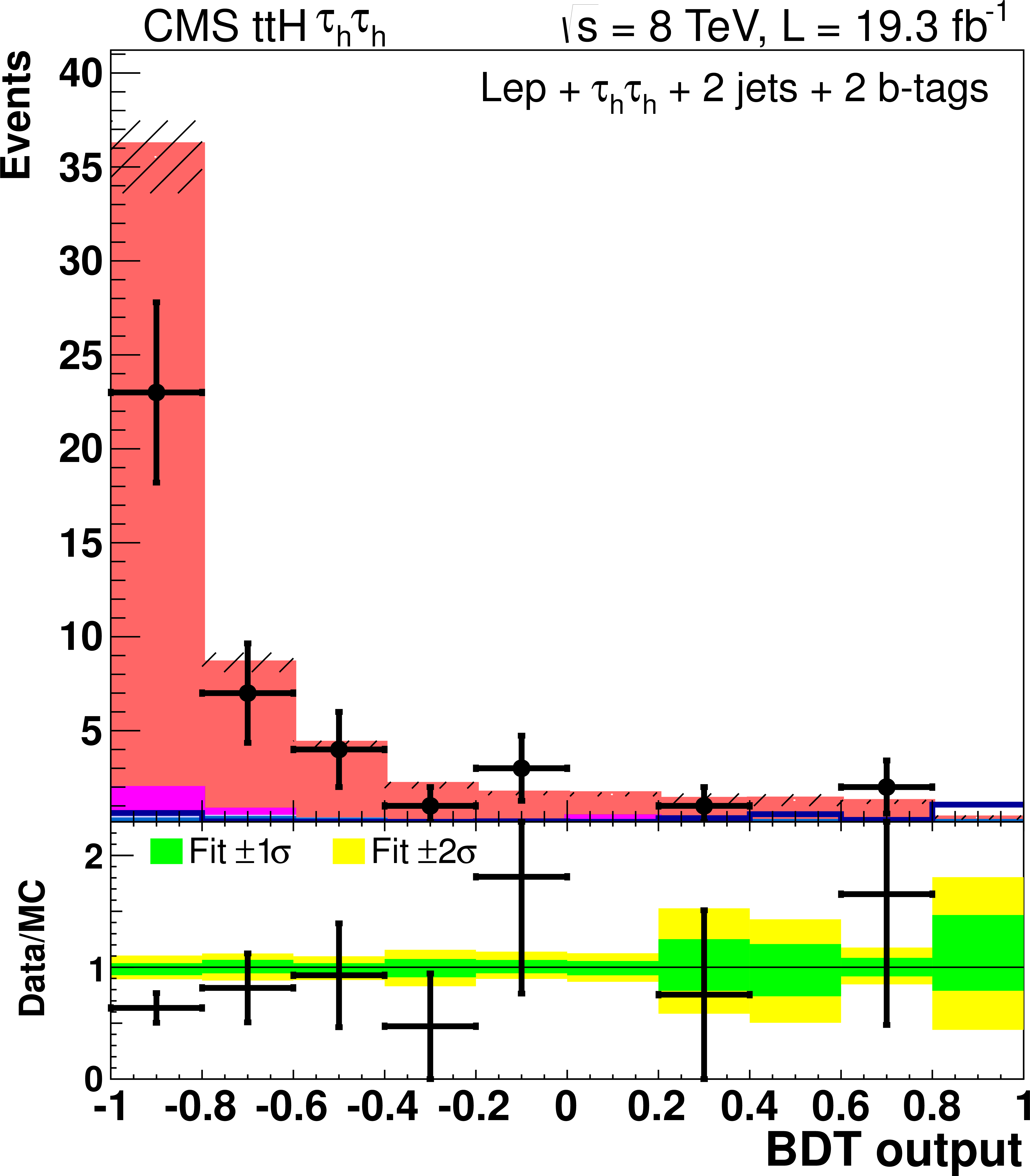
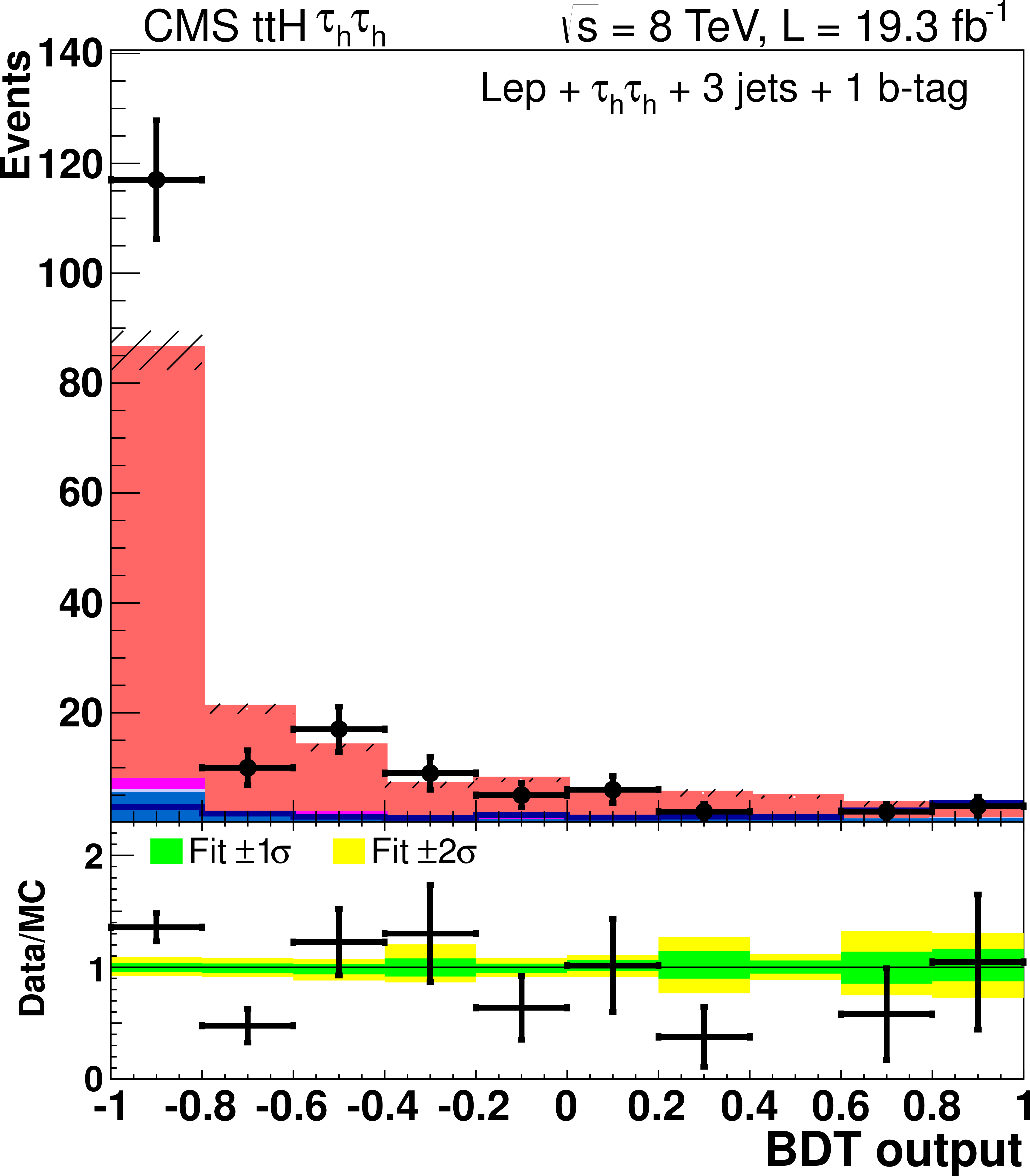
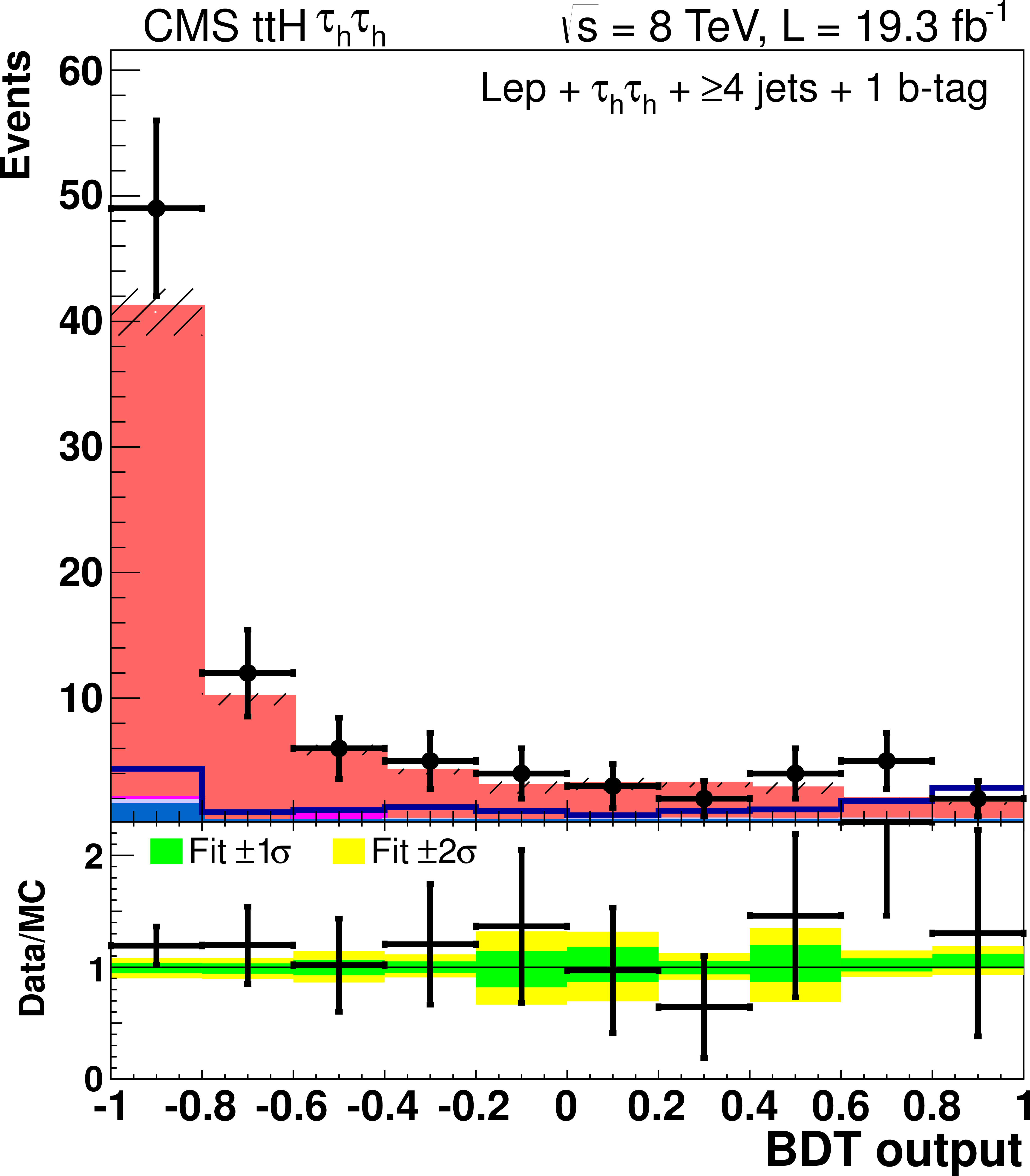
Figure 7-a:
Final BDT output for events in the $ {\tau _\mathrm {h}} $ channel. The top row is the 2 jet categories, while the second and third rows are for the categories with 3 jets and $\geq $4 jets, respectively. In each row, the columns are for the categories with 1 b-tag (left) and 2 b-tags (right). Details regarding signal and background normalizations are described in the text. |
png pdf |
Figure 7-b:
Final BDT output for events in the $ {\tau _\mathrm {h}} $ channel. The top row is the 2 jet categories, while the second and third rows are for the categories with 3 jets and $\geq $4 jets, respectively. In each row, the columns are for the categories with 1 b-tag (left) and 2 b-tags (right). Details regarding signal and background normalizations are described in the text. |
png pdf |
Figure 7-c:
Final BDT output for events in the $ {\tau _\mathrm {h}} $ channel. The top row is the 2 jet categories, while the second and third rows are for the categories with 3 jets and $\geq $4 jets, respectively. In each row, the columns are for the categories with 1 b-tag (left) and 2 b-tags (right). Details regarding signal and background normalizations are described in the text. |

png pdf |
Figure 7-d:
Final BDT output for events in the $ {\tau _\mathrm {h}} $ channel. The top row is the 2 jet categories, while the second and third rows are for the categories with 3 jets and $\geq $4 jets, respectively. In each row, the columns are for the categories with 1 b-tag (left) and 2 b-tags (right). Details regarding signal and background normalizations are described in the text. |
png pdf |
Figure 7-e:
Final BDT output for events in the $ {\tau _\mathrm {h}} $ channel. The top row is the 2 jet categories, while the second and third rows are for the categories with 3 jets and $\geq $4 jets, respectively. In each row, the columns are for the categories with 1 b-tag (left) and 2 b-tags (right). Details regarding signal and background normalizations are described in the text. |
png pdf |
Figure 7-f:
Final BDT output for events in the $ {\tau _\mathrm {h}} $ channel. The top row is the 2 jet categories, while the second and third rows are for the categories with 3 jets and $\geq $4 jets, respectively. In each row, the columns are for the categories with 1 b-tag (left) and 2 b-tags (right). Details regarding signal and background normalizations are described in the text. |

png pdf |
Figure 7-g:
Final BDT output for events in the $ {\tau _\mathrm {h}} $ channel. The top row is the 2 jet categories, while the second and third rows are for the categories with 3 jets and $\geq $4 jets, respectively. In each row, the columns are for the categories with 1 b-tag (left) and 2 b-tags (right). Details regarding signal and background normalizations are described in the text. |
png pdf |
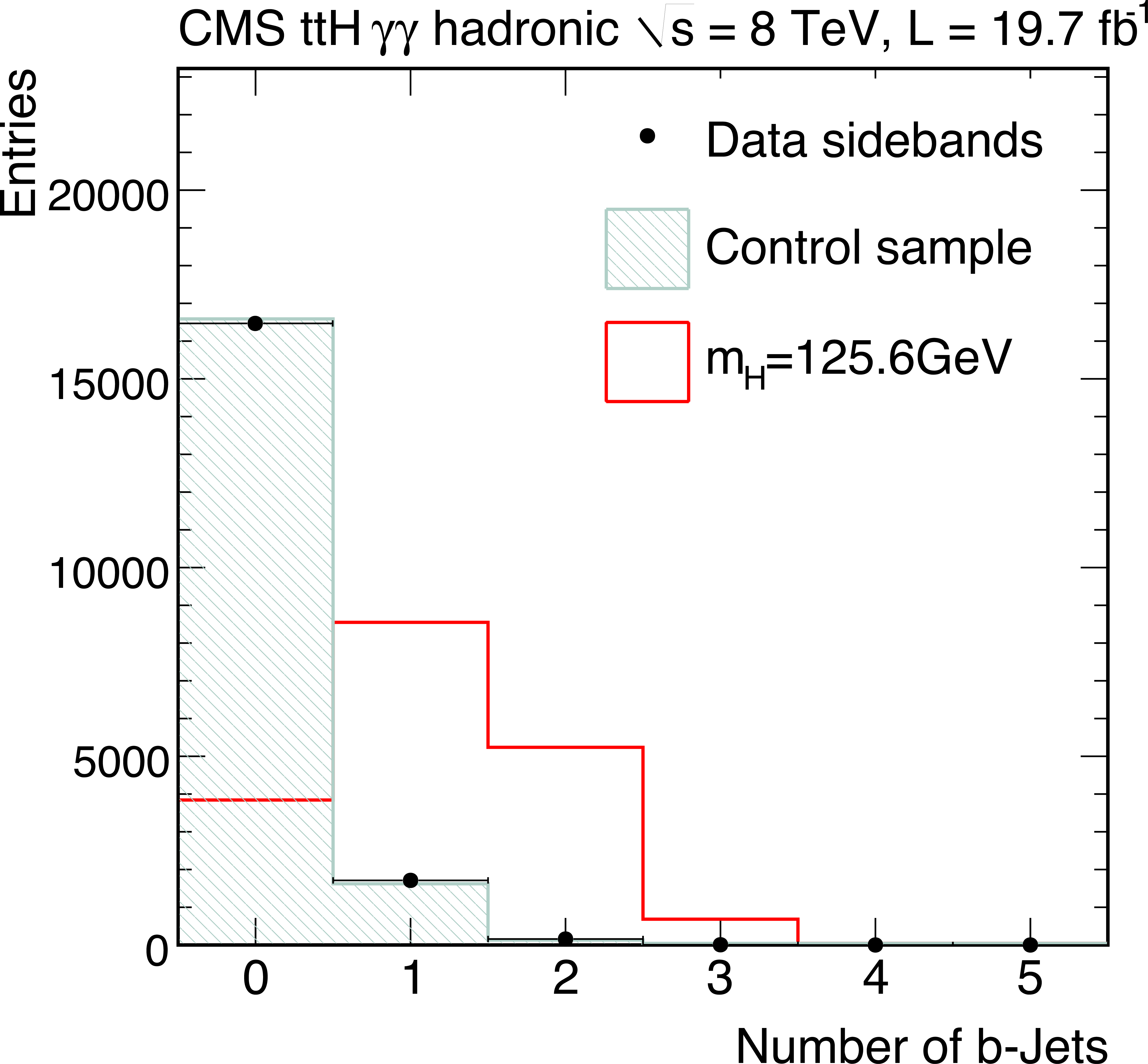
Figure 8-a:
Distributions of the b-tagged jet multiplicity (top row) and jet multiplicity (bottom row) for events passing a relaxed selection in the hadronic (left) and leptonic (right) channels, but removing events where the diphoton invariant mass is consistent with the Higgs boson mass within a 10 GeV window. The relaxed selection applies the standard photon and lepton requirements but allows events with any number of jets. The plots compare the data events with two photons and at least two jets (black markers) and the data from the control sample (green filled histogram) to simulated $ {\mathrm {t}\overline {\mathrm {t}}} {\mathrm {H}} $ events (red open histogram). Both signal and background histograms are normalized to the total number of data events observed in this region to allow for a shape comparison. |
png pdf |
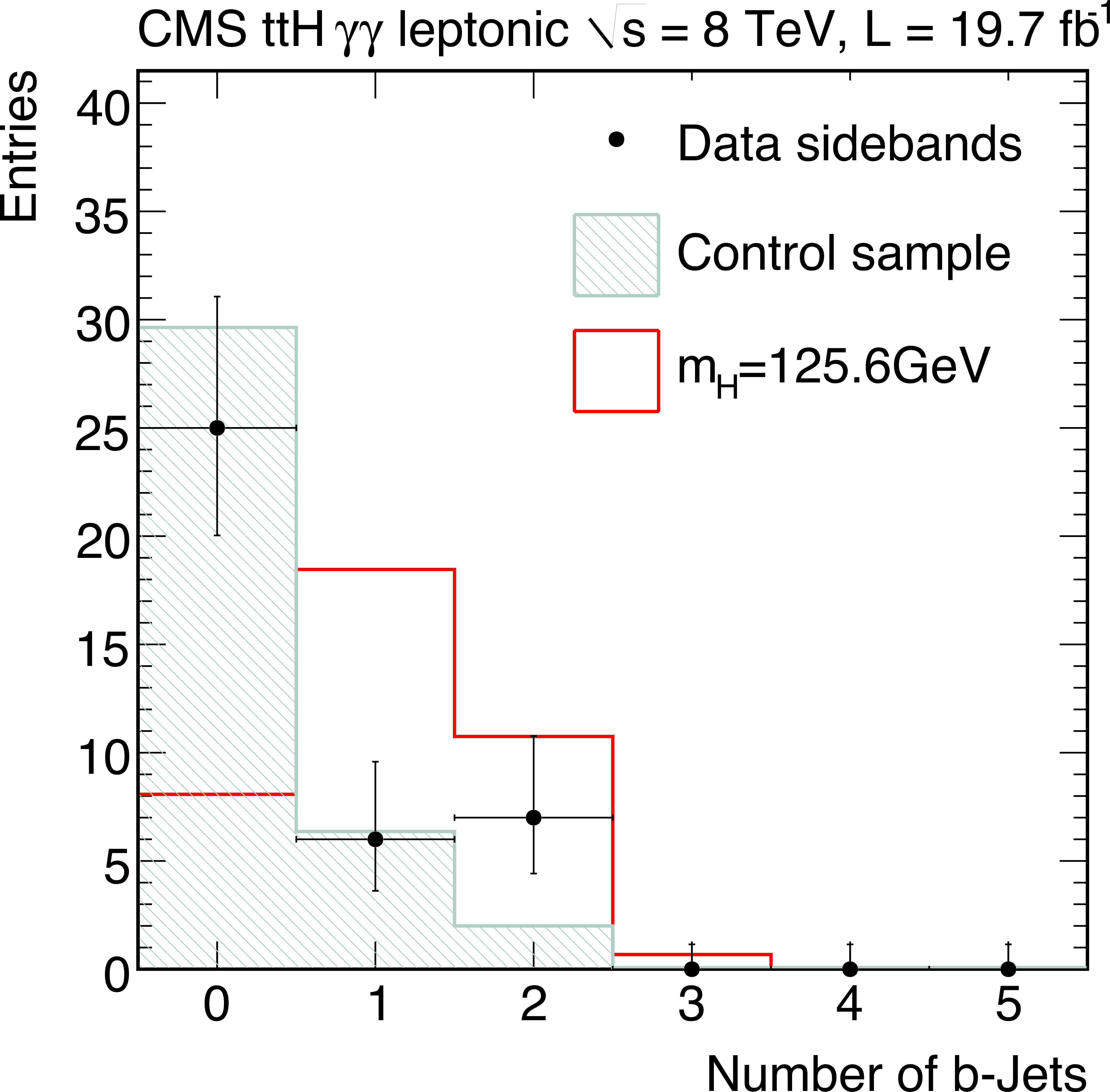
Figure 8-b:
Distributions of the b-tagged jet multiplicity (top row) and jet multiplicity (bottom row) for events passing a relaxed selection in the hadronic (left) and leptonic (right) channels, but removing events where the diphoton invariant mass is consistent with the Higgs boson mass within a 10 GeV window. The relaxed selection applies the standard photon and lepton requirements but allows events with any number of jets. The plots compare the data events with two photons and at least two jets (black markers) and the data from the control sample (green filled histogram) to simulated $ {\mathrm {t}\overline {\mathrm {t}}} {\mathrm {H}} $ events (red open histogram). Both signal and background histograms are normalized to the total number of data events observed in this region to allow for a shape comparison. |

png pdf |
Figure 8-c:
Distributions of the b-tagged jet multiplicity (top row) and jet multiplicity (bottom row) for events passing a relaxed selection in the hadronic (left) and leptonic (right) channels, but removing events where the diphoton invariant mass is consistent with the Higgs boson mass within a 10 GeV window. The relaxed selection applies the standard photon and lepton requirements but allows events with any number of jets. The plots compare the data events with two photons and at least two jets (black markers) and the data from the control sample (green filled histogram) to simulated $ {\mathrm {t}\overline {\mathrm {t}}} {\mathrm {H}} $ events (red open histogram). Both signal and background histograms are normalized to the total number of data events observed in this region to allow for a shape comparison. |

png pdf |
Figure 8-d:
Distributions of the b-tagged jet multiplicity (top row) and jet multiplicity (bottom row) for events passing a relaxed selection in the hadronic (left) and leptonic (right) channels, but removing events where the diphoton invariant mass is consistent with the Higgs boson mass within a 10 GeV window. The relaxed selection applies the standard photon and lepton requirements but allows events with any number of jets. The plots compare the data events with two photons and at least two jets (black markers) and the data from the control sample (green filled histogram) to simulated $ {\mathrm {t}\overline {\mathrm {t}}} {\mathrm {H}} $ events (red open histogram). Both signal and background histograms are normalized to the total number of data events observed in this region to allow for a shape comparison. |
png pdf |
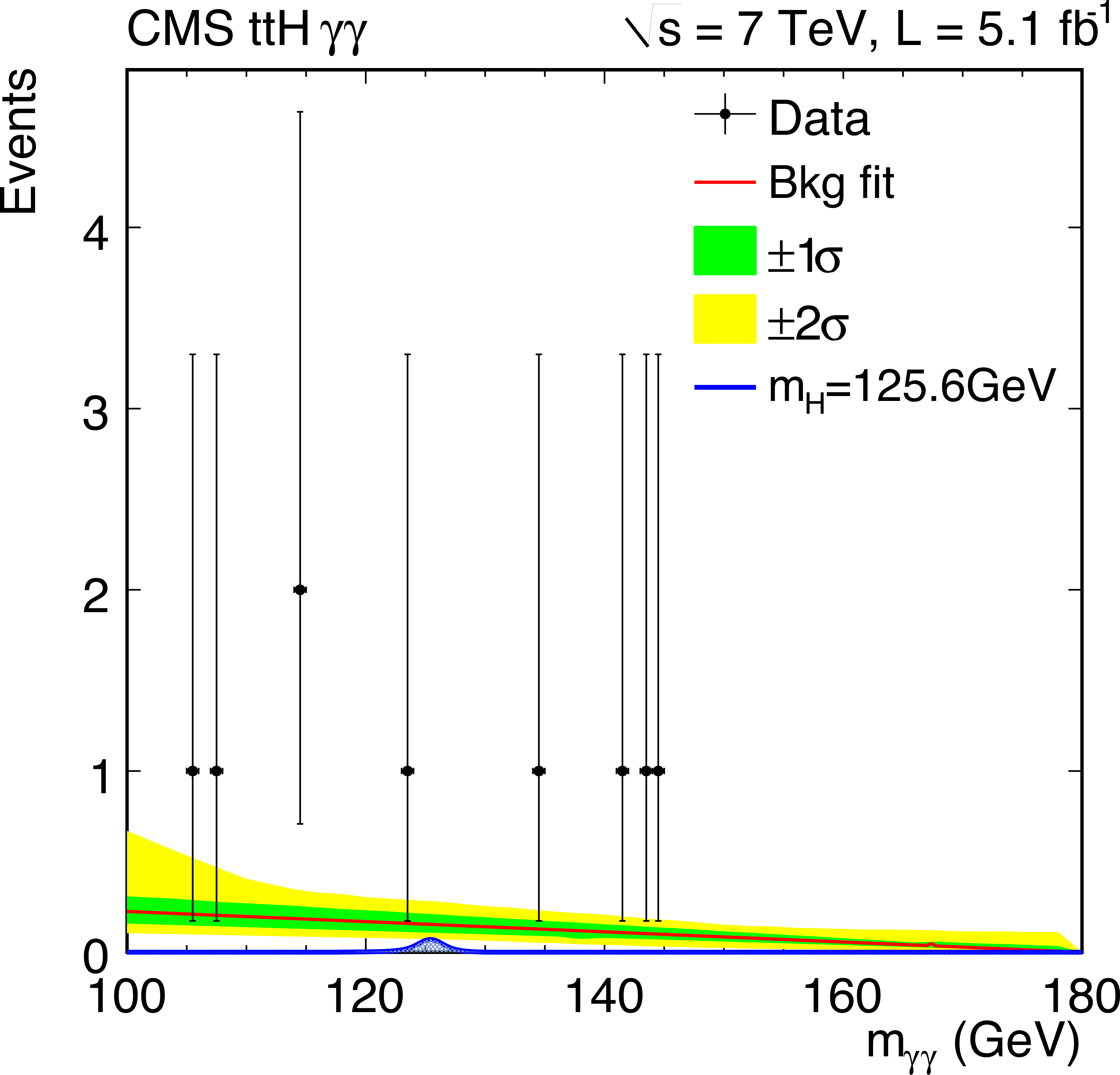
Figure 9-a:
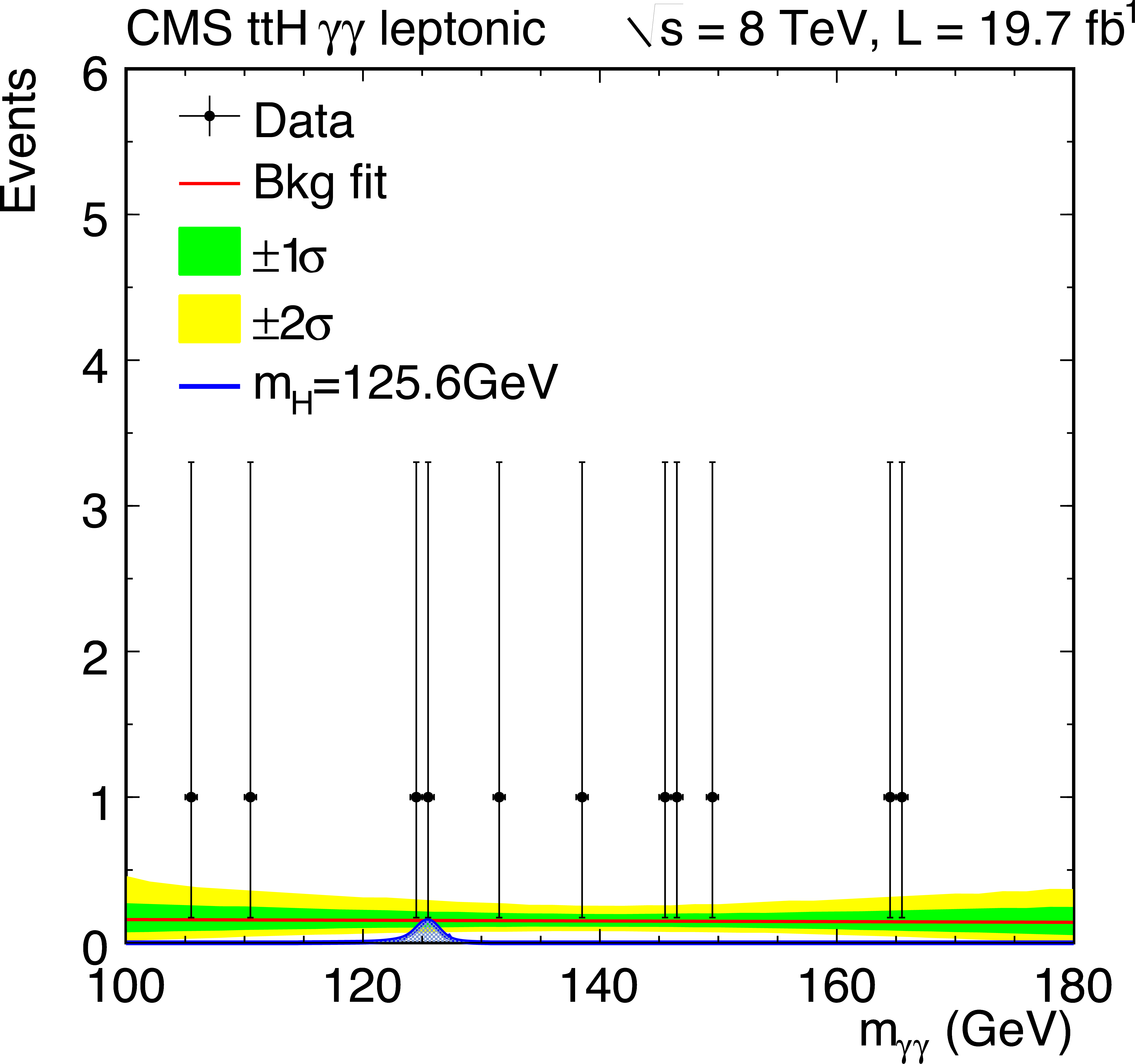
Diphoton invariant mass distribution for $\sqrt {s} = 7 TeV $ data events for the combined hadronic and leptonic selections on the left, and for $\sqrt {s} = 8 TeV $ data events passing the hadronic (middle), and leptonic (right) selections. The red line represents the fit to the data, while the green (yellow) band show the $1 \sigma $ ($2 \sigma $) uncertainty band. The theoretical prediction for the signal contribution (in blue) includes the main Higgs boson production modes. |
png pdf |
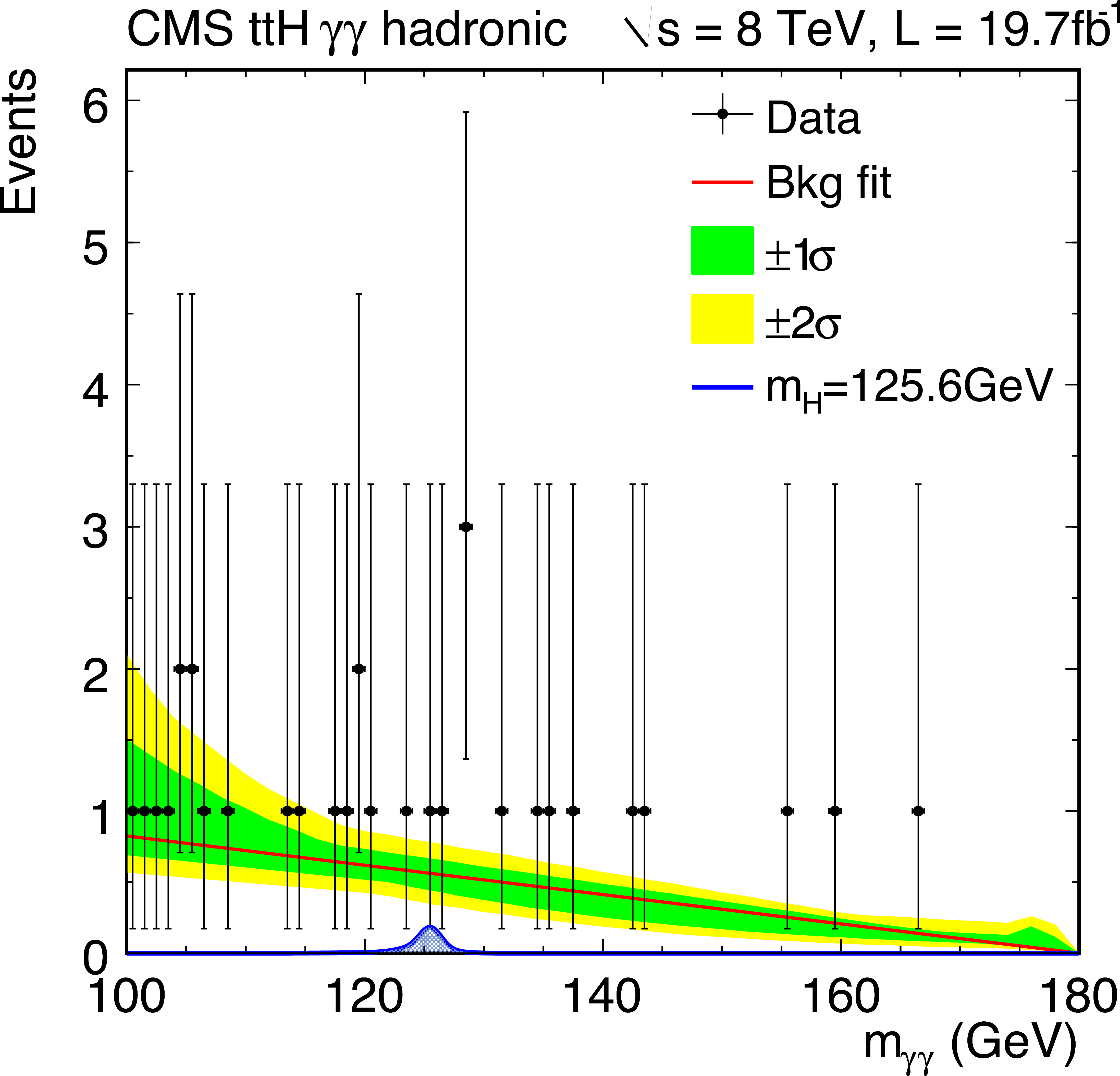
Figure 9-b:
Diphoton invariant mass distribution for $\sqrt {s} = 7 TeV $ data events for the combined hadronic and leptonic selections on the left, and for $\sqrt {s} = 8 TeV $ data events passing the hadronic (middle), and leptonic (right) selections. The red line represents the fit to the data, while the green (yellow) band show the $1 \sigma $ ($2 \sigma $) uncertainty band. The theoretical prediction for the signal contribution (in blue) includes the main Higgs boson production modes. |
png pdf |
Figure 9-c:
Diphoton invariant mass distribution for $\sqrt {s} = 7 TeV $ data events for the combined hadronic and leptonic selections on the left, and for $\sqrt {s} = 8 TeV $ data events passing the hadronic (middle), and leptonic (right) selections. The red line represents the fit to the data, while the green (yellow) band show the $1 \sigma $ ($2 \sigma $) uncertainty band. The theoretical prediction for the signal contribution (in blue) includes the main Higgs boson production modes. |
png pdf |
Figure 10-a:
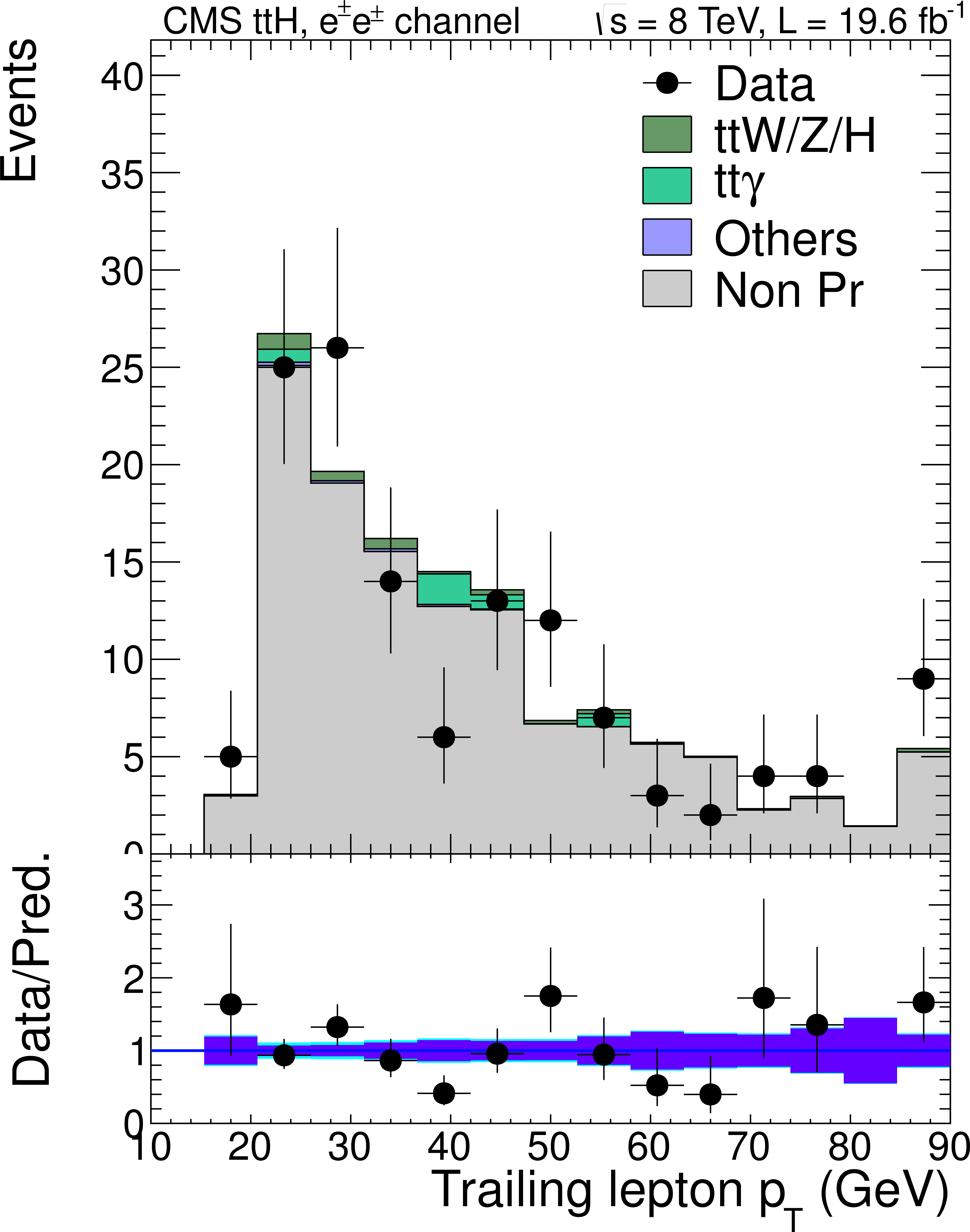
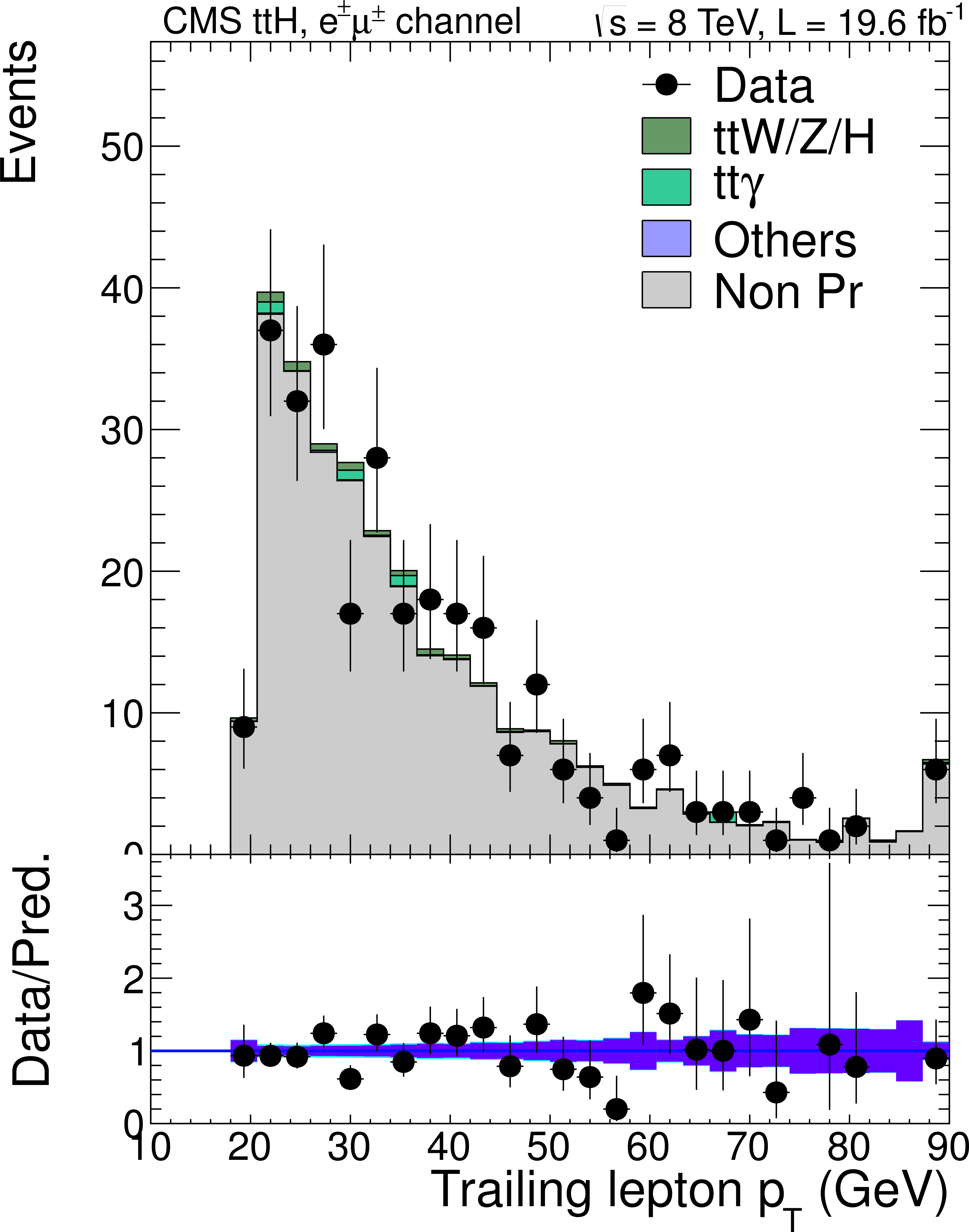
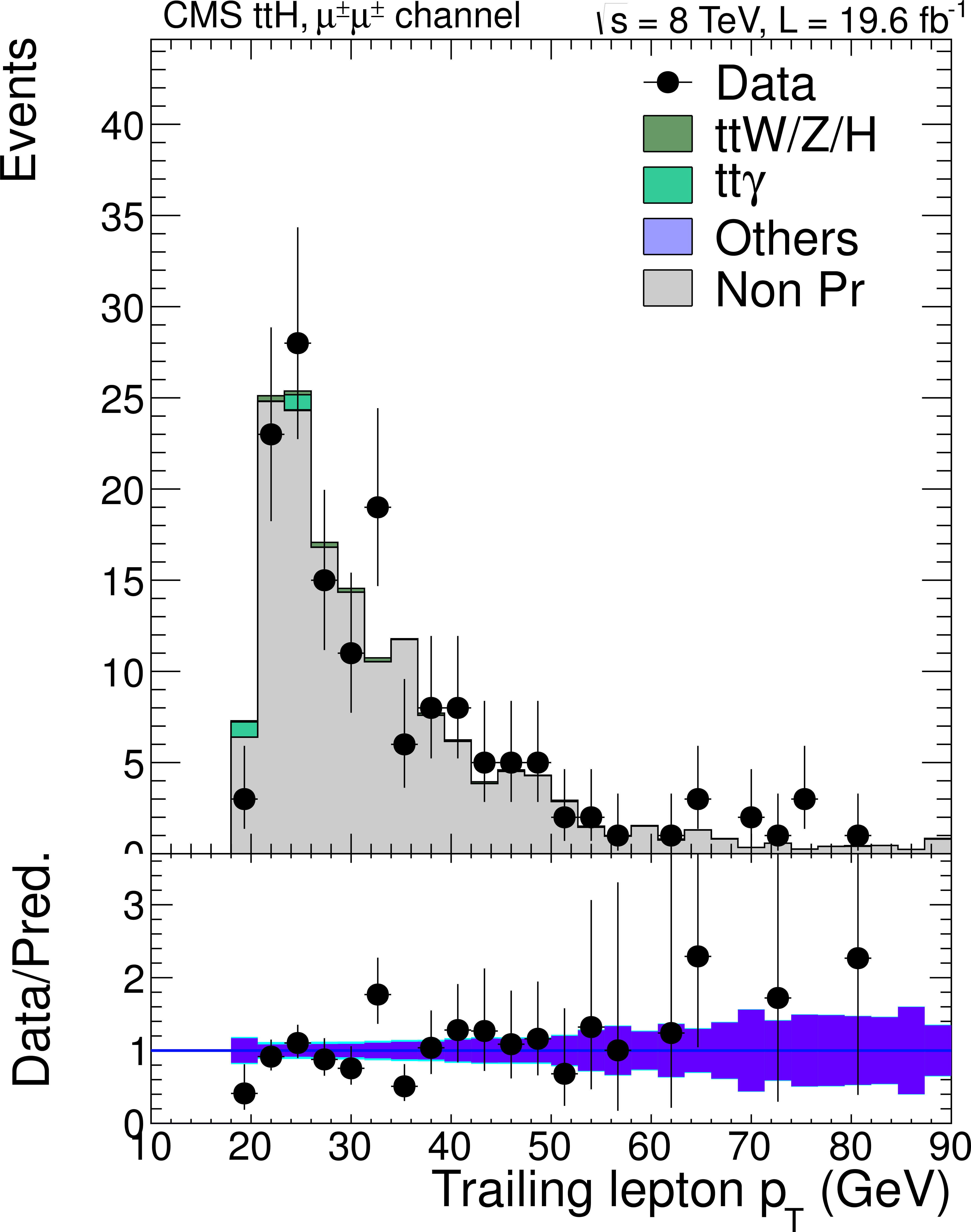
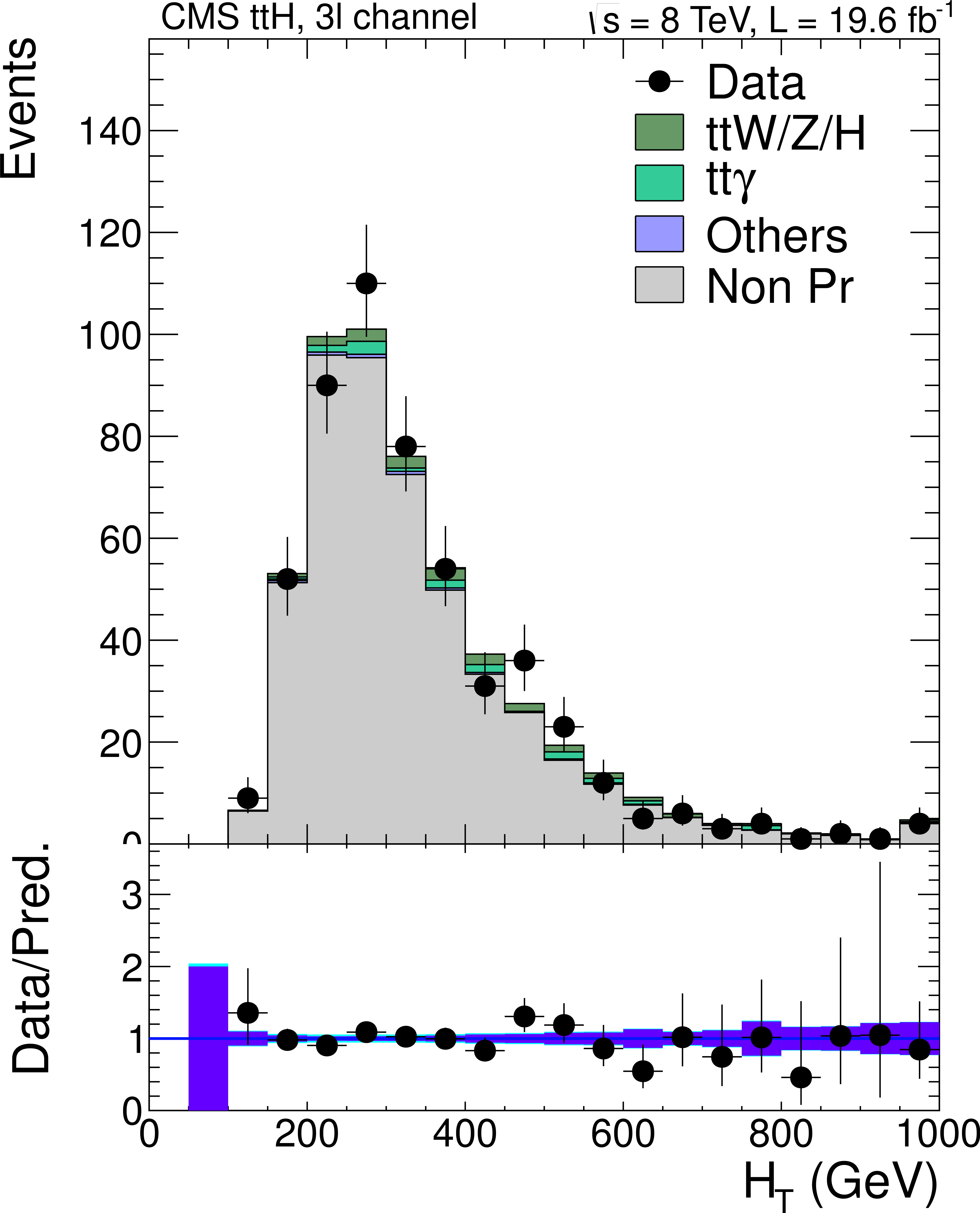
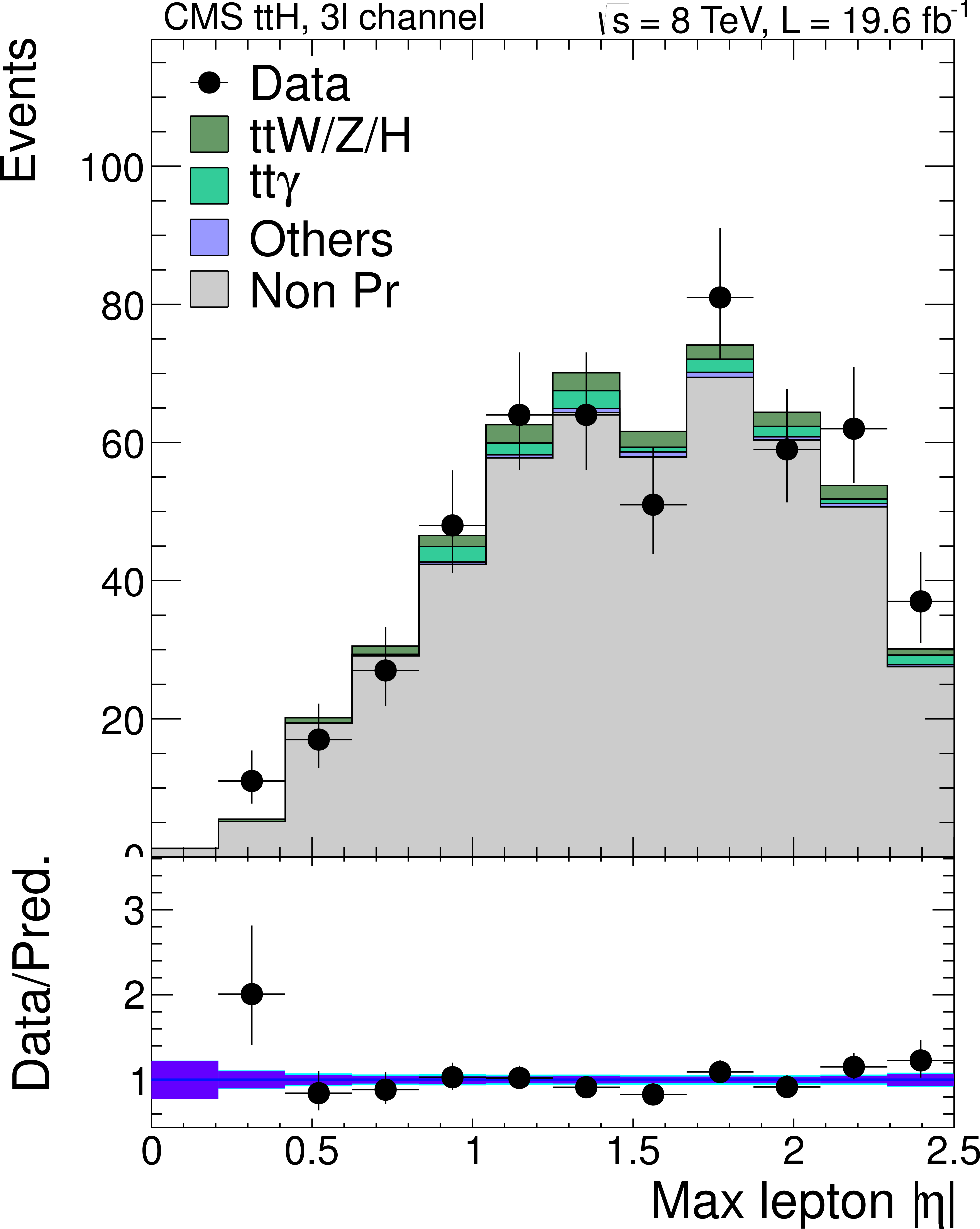
These plots show the distribution of key discriminating variables for events where one lepton fails the lepton MVA requirement. The expected distribution for the non-prompt background is taken from simulation (mostly $ {\mathrm {t}\overline {\mathrm {t}}} $+jets), and the yield is fitted from the data. The bottom panel of each plot shows the ratio between data and predictions as well as the overall uncertainties after the fit (blue). In the first row the distributions of the trailing lepton $ {p_{\mathrm {T}}} $ for the $ {\mathrm {e}}^{\pm } {\mathrm {e}}^{\pm }$ (left), $ {\mathrm {e}}^{\pm }\mu ^{\pm }$ (center), and $\mu ^{\pm }\mu ^{\pm }$ (right) final states are shown. In the second row the distributions of the $H_\mathrm {T}$ (left), the $ {p_{\mathrm {T}}} $ of the jet with highest b-tagging discriminator (center), and the lepton maximum $ {| \eta | }$ (right) are shown for the trilepton channel. |
png pdf |
Figure 10-b:
These plots show the distribution of key discriminating variables for events where one lepton fails the lepton MVA requirement. The expected distribution for the non-prompt background is taken from simulation (mostly $ {\mathrm {t}\overline {\mathrm {t}}} $+jets), and the yield is fitted from the data. The bottom panel of each plot shows the ratio between data and predictions as well as the overall uncertainties after the fit (blue). In the first row the distributions of the trailing lepton $ {p_{\mathrm {T}}} $ for the $ {\mathrm {e}}^{\pm } {\mathrm {e}}^{\pm }$ (left), $ {\mathrm {e}}^{\pm }\mu ^{\pm }$ (center), and $\mu ^{\pm }\mu ^{\pm }$ (right) final states are shown. In the second row the distributions of the $H_\mathrm {T}$ (left), the $ {p_{\mathrm {T}}} $ of the jet with highest b-tagging discriminator (center), and the lepton maximum $ {| \eta | }$ (right) are shown for the trilepton channel. |
png pdf |
Figure 10-c:
These plots show the distribution of key discriminating variables for events where one lepton fails the lepton MVA requirement. The expected distribution for the non-prompt background is taken from simulation (mostly $ {\mathrm {t}\overline {\mathrm {t}}} $+jets), and the yield is fitted from the data. The bottom panel of each plot shows the ratio between data and predictions as well as the overall uncertainties after the fit (blue). In the first row the distributions of the trailing lepton $ {p_{\mathrm {T}}} $ for the $ {\mathrm {e}}^{\pm } {\mathrm {e}}^{\pm }$ (left), $ {\mathrm {e}}^{\pm }\mu ^{\pm }$ (center), and $\mu ^{\pm }\mu ^{\pm }$ (right) final states are shown. In the second row the distributions of the $H_\mathrm {T}$ (left), the $ {p_{\mathrm {T}}} $ of the jet with highest b-tagging discriminator (center), and the lepton maximum $ {| \eta | }$ (right) are shown for the trilepton channel. |
png pdf |
Figure 10-d:
These plots show the distribution of key discriminating variables for events where one lepton fails the lepton MVA requirement. The expected distribution for the non-prompt background is taken from simulation (mostly $ {\mathrm {t}\overline {\mathrm {t}}} $+jets), and the yield is fitted from the data. The bottom panel of each plot shows the ratio between data and predictions as well as the overall uncertainties after the fit (blue). In the first row the distributions of the trailing lepton $ {p_{\mathrm {T}}} $ for the $ {\mathrm {e}}^{\pm } {\mathrm {e}}^{\pm }$ (left), $ {\mathrm {e}}^{\pm }\mu ^{\pm }$ (center), and $\mu ^{\pm }\mu ^{\pm }$ (right) final states are shown. In the second row the distributions of the $H_\mathrm {T}$ (left), the $ {p_{\mathrm {T}}} $ of the jet with highest b-tagging discriminator (center), and the lepton maximum $ {| \eta | }$ (right) are shown for the trilepton channel. |

png pdf |
Figure 10-e:
These plots show the distribution of key discriminating variables for events where one lepton fails the lepton MVA requirement. The expected distribution for the non-prompt background is taken from simulation (mostly $ {\mathrm {t}\overline {\mathrm {t}}} $+jets), and the yield is fitted from the data. The bottom panel of each plot shows the ratio between data and predictions as well as the overall uncertainties after the fit (blue). In the first row the distributions of the trailing lepton $ {p_{\mathrm {T}}} $ for the $ {\mathrm {e}}^{\pm } {\mathrm {e}}^{\pm }$ (left), $ {\mathrm {e}}^{\pm }\mu ^{\pm }$ (center), and $\mu ^{\pm }\mu ^{\pm }$ (right) final states are shown. In the second row the distributions of the $H_\mathrm {T}$ (left), the $ {p_{\mathrm {T}}} $ of the jet with highest b-tagging discriminator (center), and the lepton maximum $ {| \eta | }$ (right) are shown for the trilepton channel. |
png pdf |
Figure 10-f:
These plots show the distribution of key discriminating variables for events where one lepton fails the lepton MVA requirement. The expected distribution for the non-prompt background is taken from simulation (mostly $ {\mathrm {t}\overline {\mathrm {t}}} $+jets), and the yield is fitted from the data. The bottom panel of each plot shows the ratio between data and predictions as well as the overall uncertainties after the fit (blue). In the first row the distributions of the trailing lepton $ {p_{\mathrm {T}}} $ for the $ {\mathrm {e}}^{\pm } {\mathrm {e}}^{\pm }$ (left), $ {\mathrm {e}}^{\pm }\mu ^{\pm }$ (center), and $\mu ^{\pm }\mu ^{\pm }$ (right) final states are shown. In the second row the distributions of the $H_\mathrm {T}$ (left), the $ {p_{\mathrm {T}}} $ of the jet with highest b-tagging discriminator (center), and the lepton maximum $ {| \eta | }$ (right) are shown for the trilepton channel. |
png pdf |
Figure 11-a:
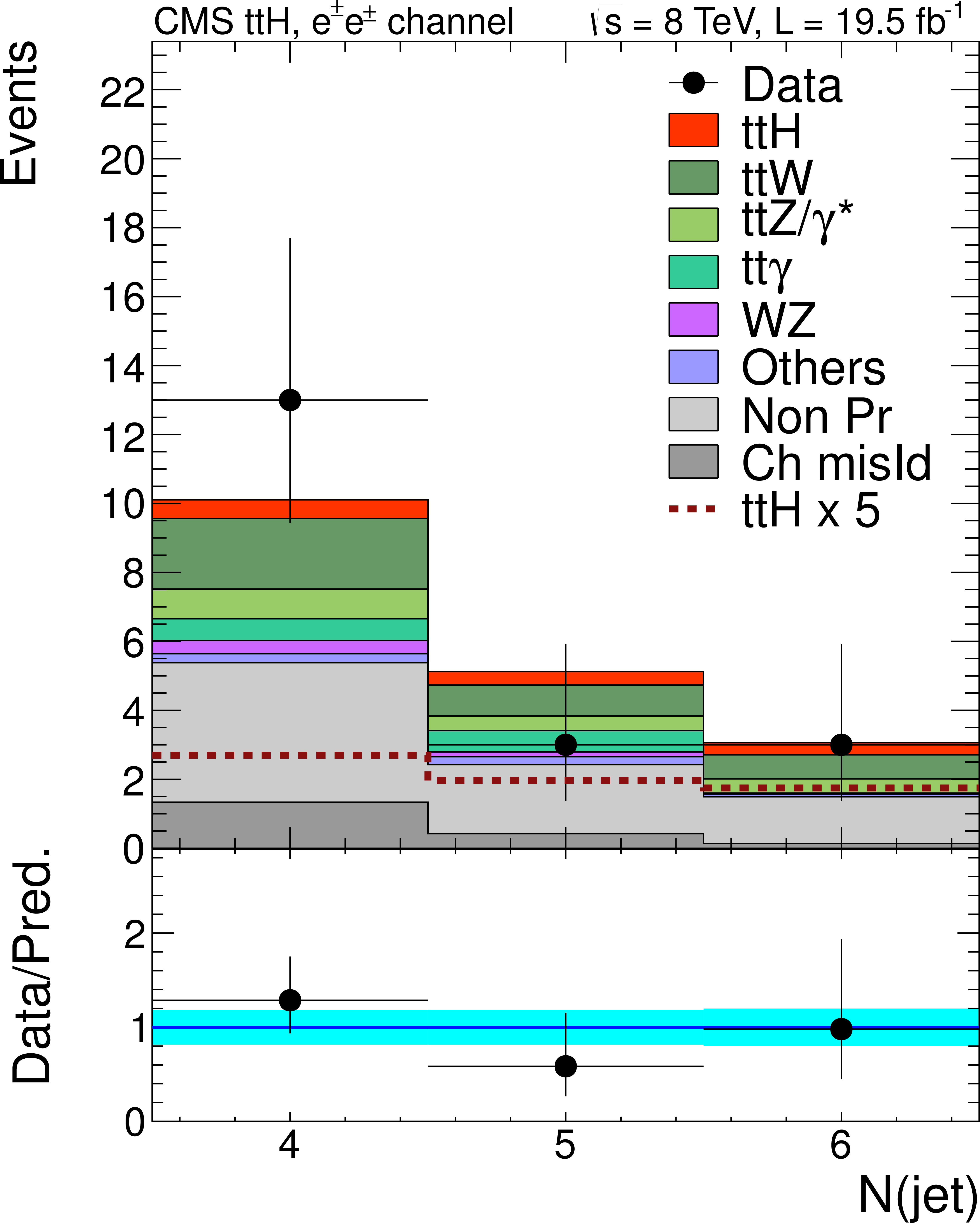
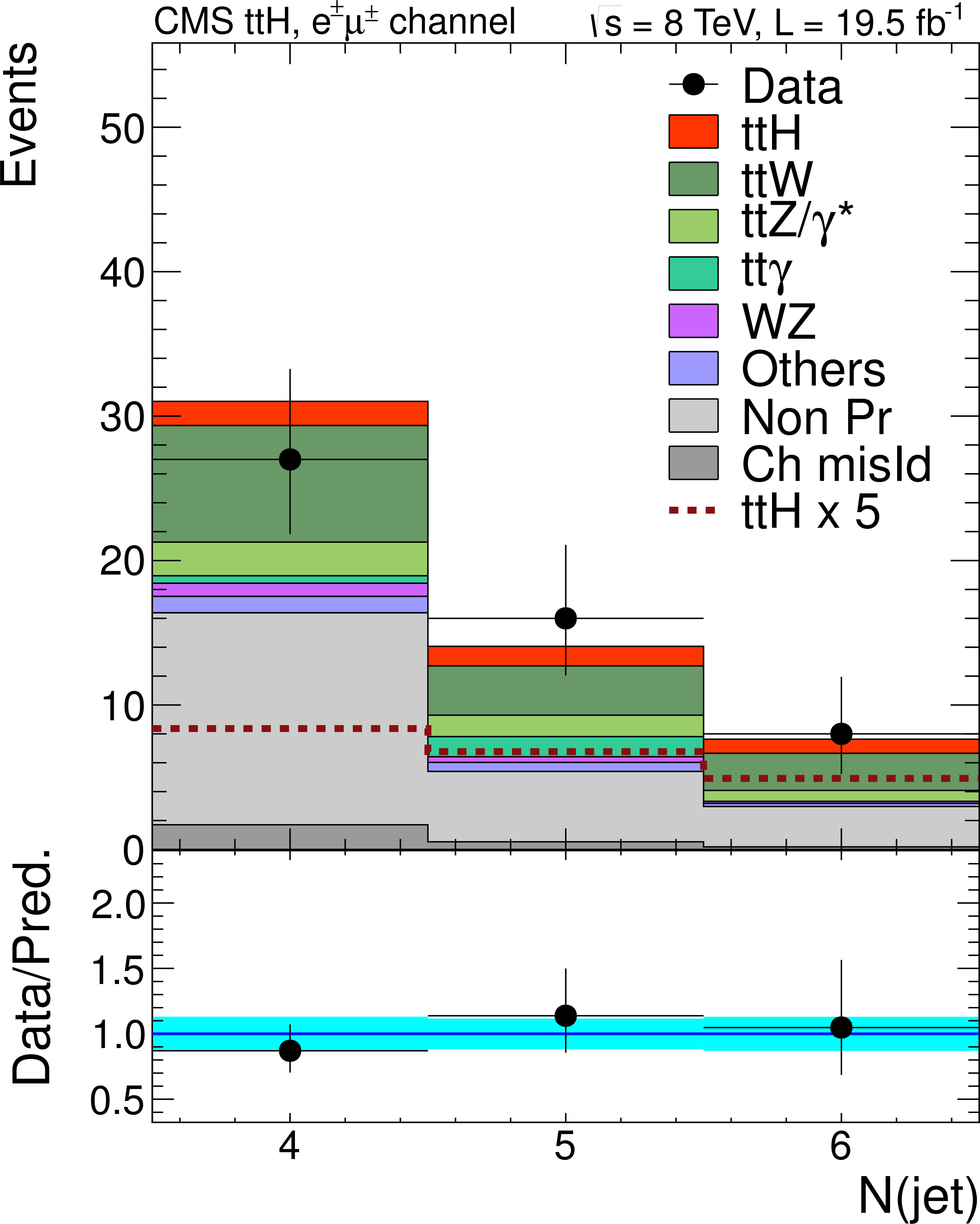
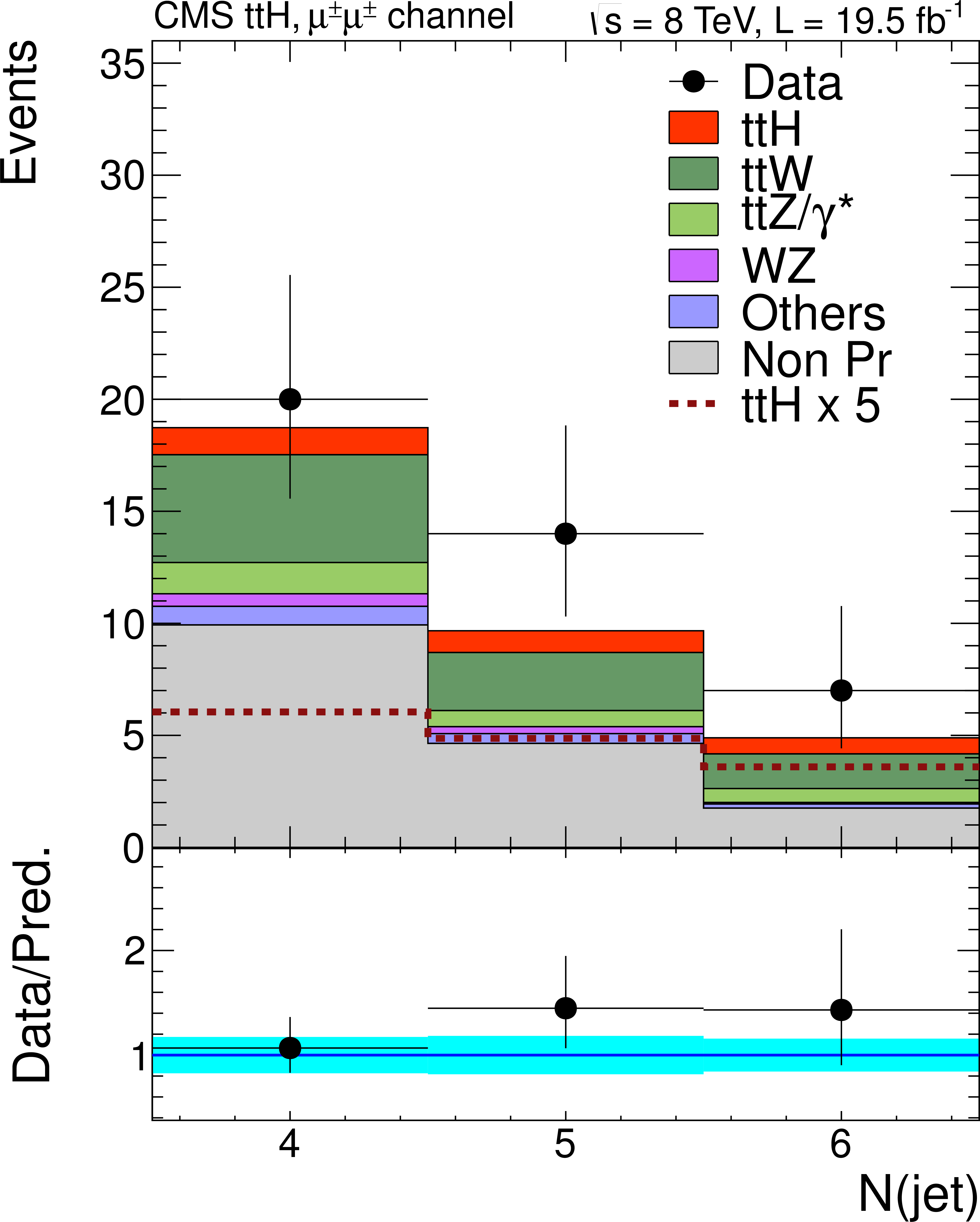
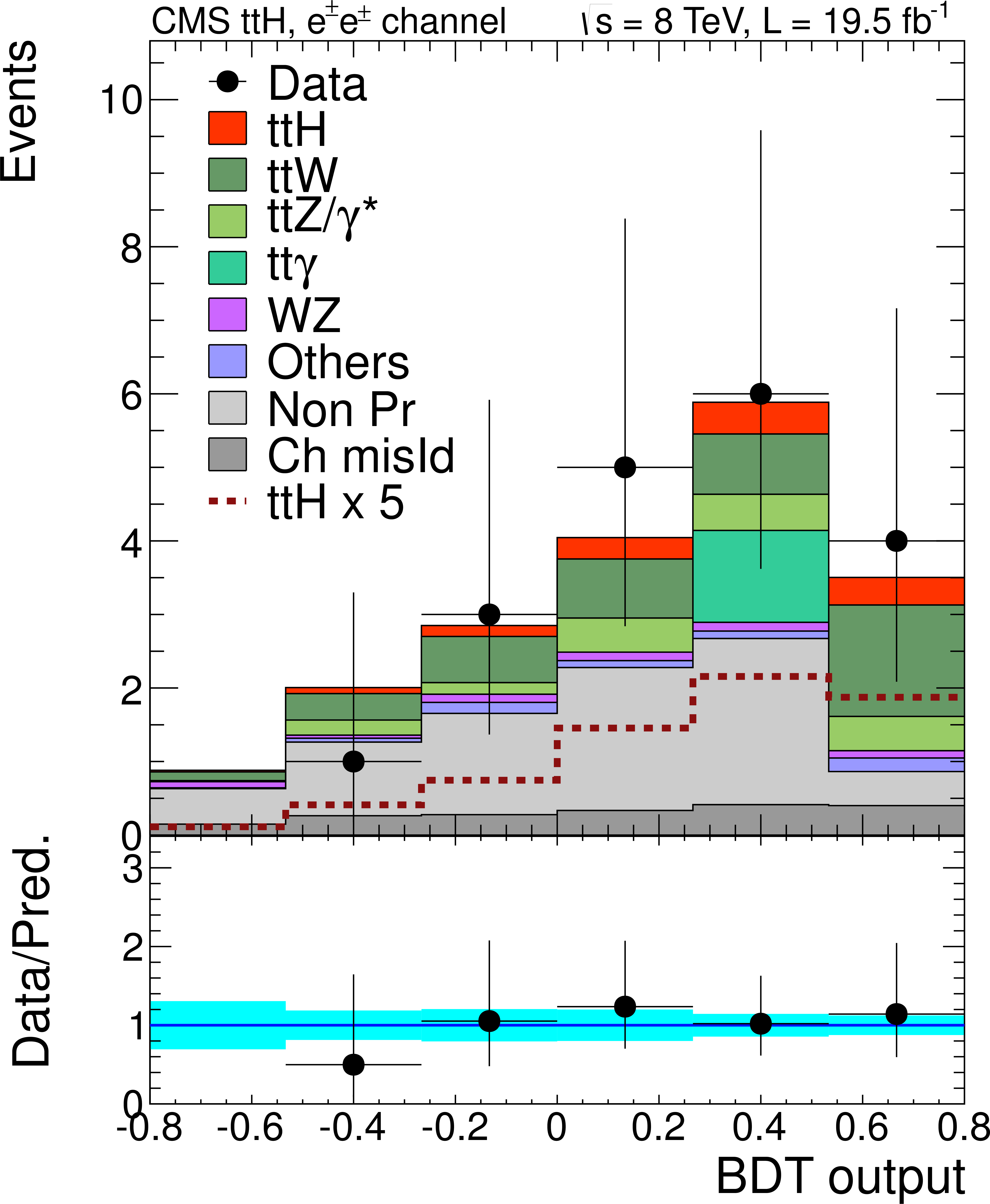
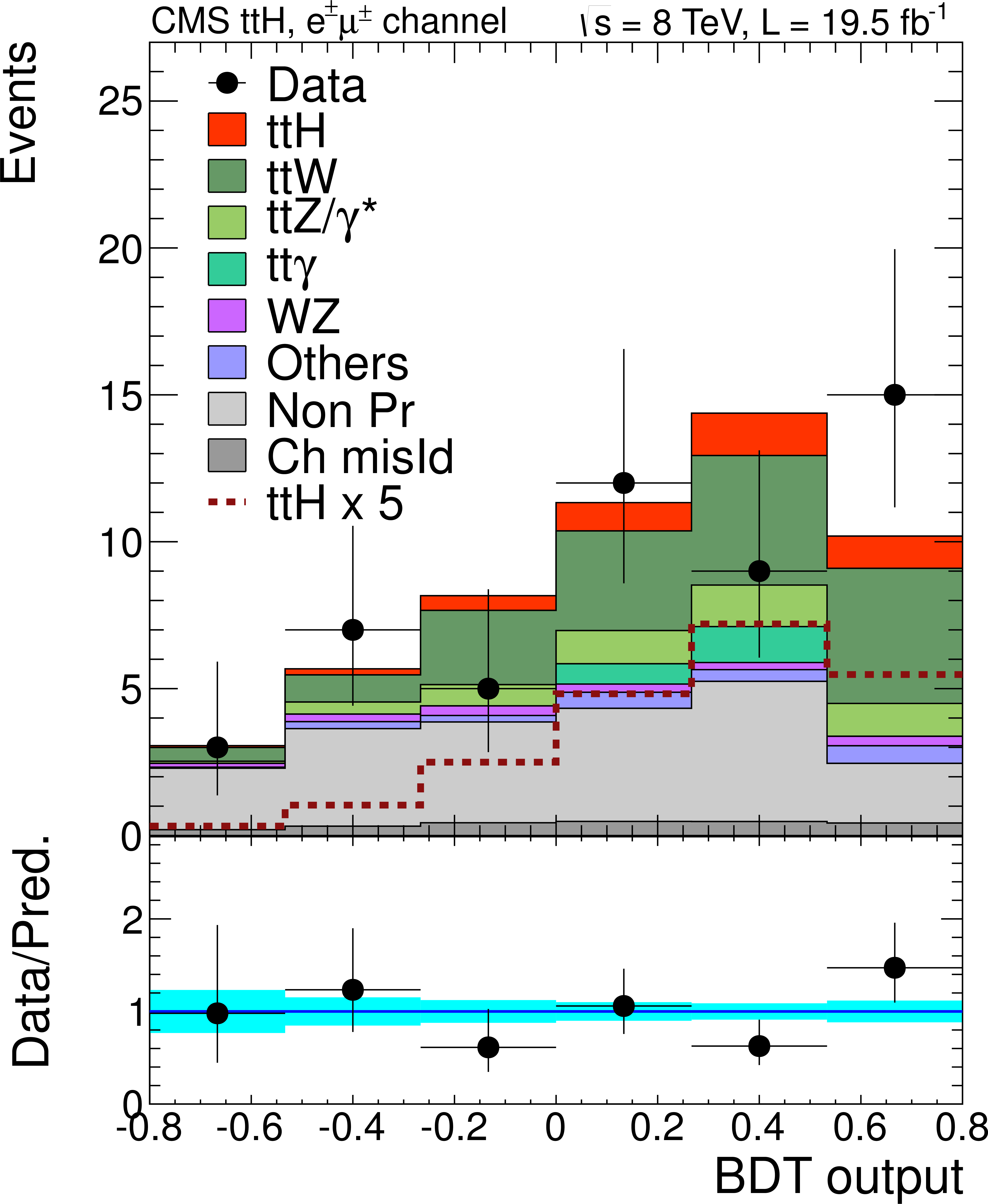
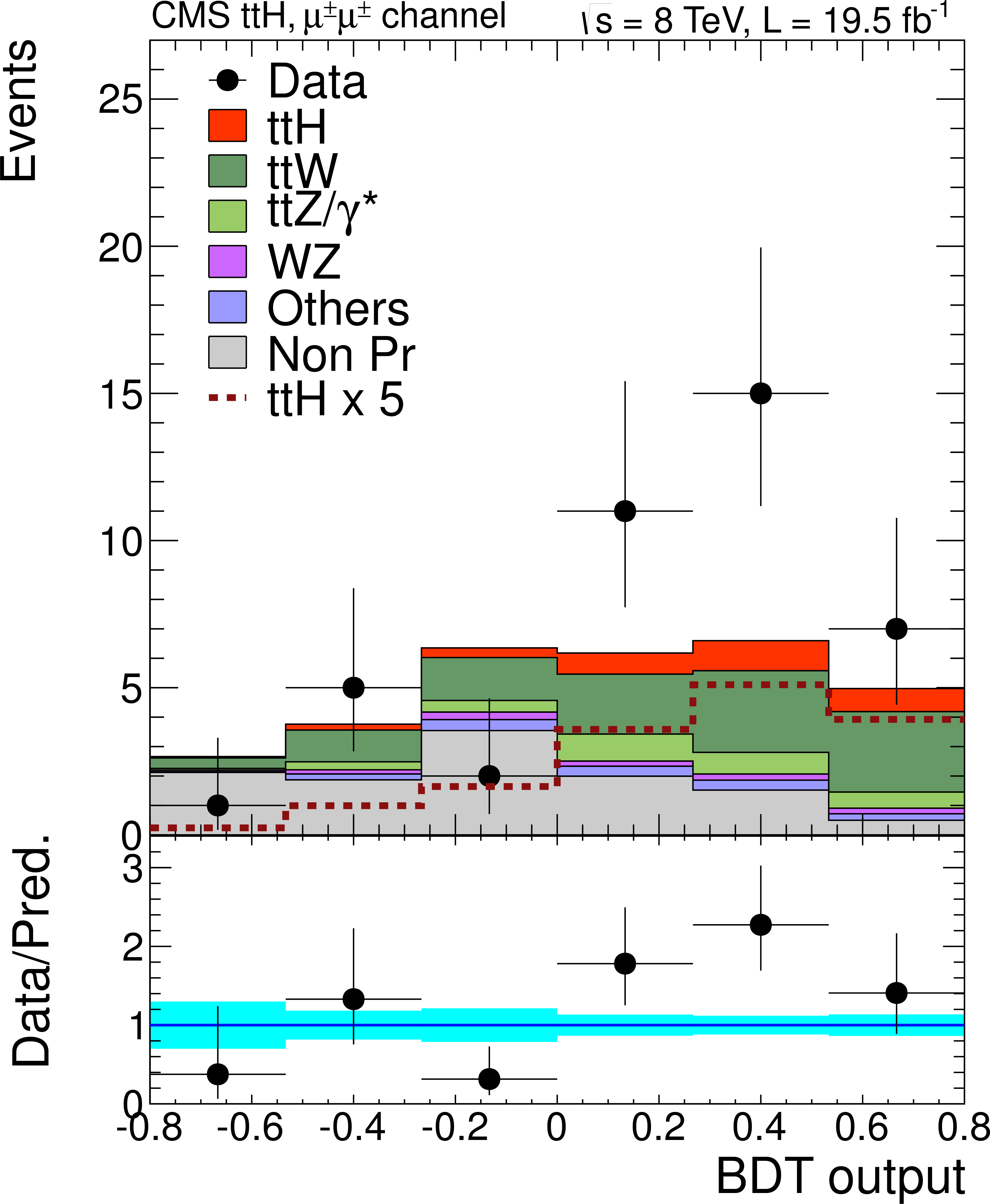
Distribution of the jet multiplicity (top row) and the BDT discriminant (bottom row) for the same-sign dilepton search, for the final states $ {\mathrm {e}} {\mathrm {e}}$ (left), $ {\mathrm {e}} {{\mu }}$ (center), and $ {{\mu }} {{\mu }}$ (right). Signal and background normalizations are explained in the text. The b-tagged jets are included in the jet multiplicity. |
png pdf |
Figure 11-b:
Distribution of the jet multiplicity (top row) and the BDT discriminant (bottom row) for the same-sign dilepton search, for the final states $ {\mathrm {e}} {\mathrm {e}}$ (left), $ {\mathrm {e}} {{\mu }}$ (center), and $ {{\mu }} {{\mu }}$ (right). Signal and background normalizations are explained in the text. The b-tagged jets are included in the jet multiplicity. |
png pdf |
Figure 11-c:
Distribution of the jet multiplicity (top row) and the BDT discriminant (bottom row) for the same-sign dilepton search, for the final states $ {\mathrm {e}} {\mathrm {e}}$ (left), $ {\mathrm {e}} {{\mu }}$ (center), and $ {{\mu }} {{\mu }}$ (right). Signal and background normalizations are explained in the text. The b-tagged jets are included in the jet multiplicity. |
png pdf |
Figure 11-d:
Distribution of the jet multiplicity (top row) and the BDT discriminant (bottom row) for the same-sign dilepton search, for the final states $ {\mathrm {e}} {\mathrm {e}}$ (left), $ {\mathrm {e}} {{\mu }}$ (center), and $ {{\mu }} {{\mu }}$ (right). Signal and background normalizations are explained in the text. The b-tagged jets are included in the jet multiplicity. |
png pdf |
Figure 11-e:
Distribution of the jet multiplicity (top row) and the BDT discriminant (bottom row) for the same-sign dilepton search, for the final states $ {\mathrm {e}} {\mathrm {e}}$ (left), $ {\mathrm {e}} {{\mu }}$ (center), and $ {{\mu }} {{\mu }}$ (right). Signal and background normalizations are explained in the text. The b-tagged jets are included in the jet multiplicity. |
png pdf |
Figure 11-f:
Distribution of the jet multiplicity (top row) and the BDT discriminant (bottom row) for the same-sign dilepton search, for the final states $ {\mathrm {e}} {\mathrm {e}}$ (left), $ {\mathrm {e}} {{\mu }}$ (center), and $ {{\mu }} {{\mu }}$ (right). Signal and background normalizations are explained in the text. The b-tagged jets are included in the jet multiplicity. |
png pdf |
Figure 12-a:
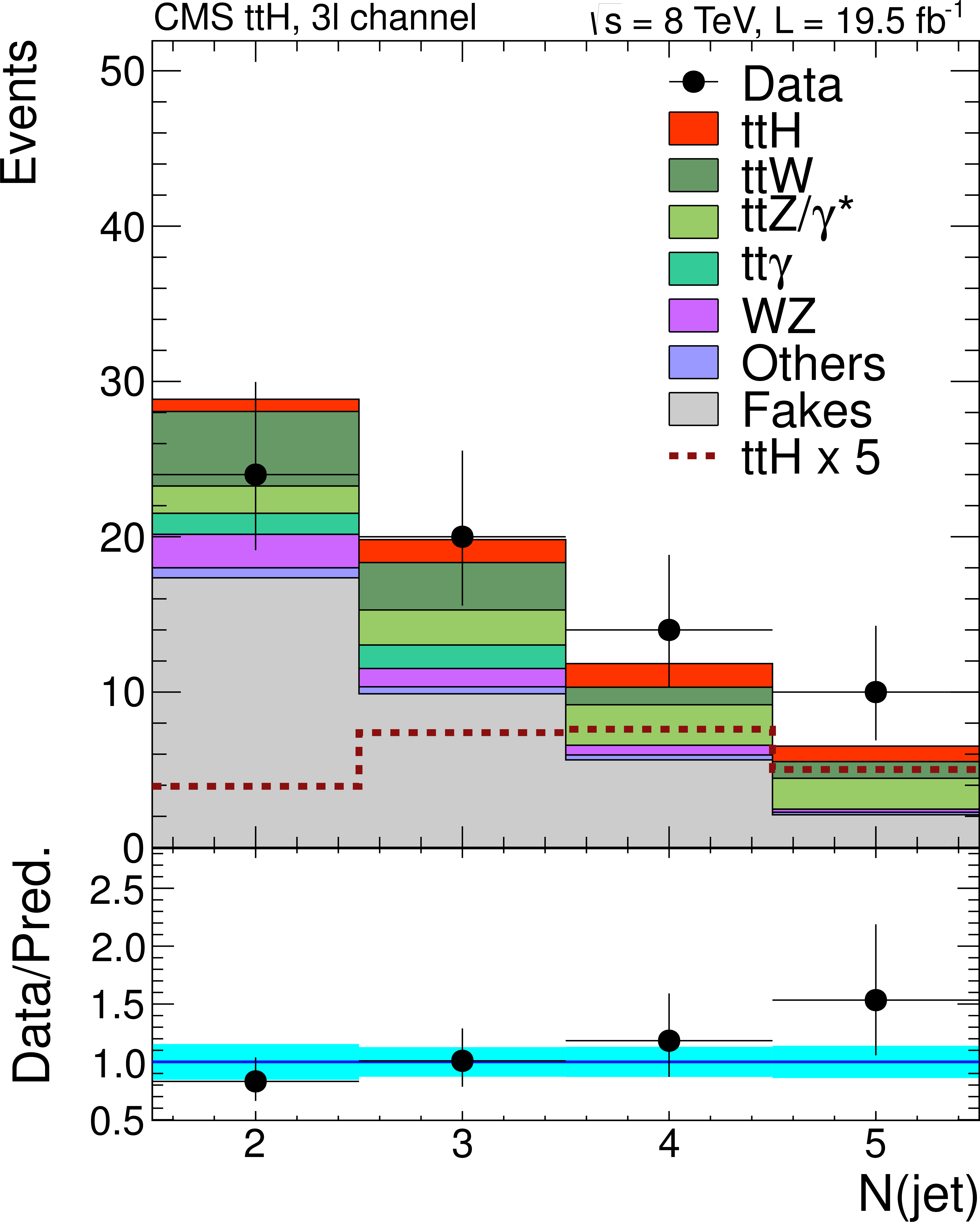
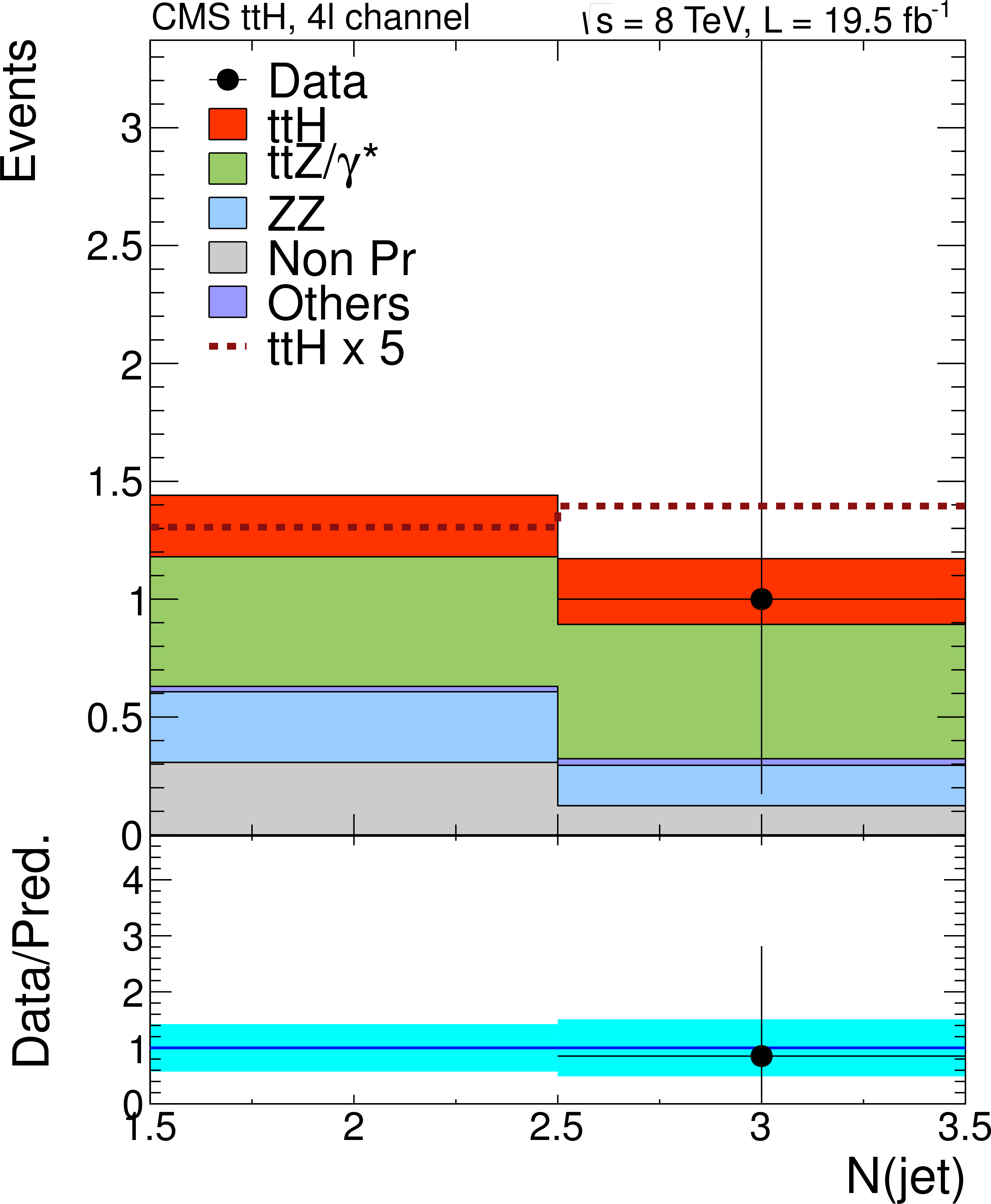
Distribution of the jet multiplicity (left) and BDT discriminant (center) for the trilepton search. Events with positive and negative charge are merged in these plots, but they are used separately in the signal extraction. The plot on the right shows the jet multiplicity for the four-lepton search. Signal and background normalizations are explained in the text. The b-tagged jets are included in the jet multiplicity. |

png pdf |
Figure 12-b:
Distribution of the jet multiplicity (left) and BDT discriminant (center) for the trilepton search. Events with positive and negative charge are merged in these plots, but they are used separately in the signal extraction. The plot on the right shows the jet multiplicity for the four-lepton search. Signal and background normalizations are explained in the text. The b-tagged jets are included in the jet multiplicity. |
png pdf |
Figure 12-c:
Distribution of the jet multiplicity (left) and BDT discriminant (center) for the trilepton search. Events with positive and negative charge are merged in these plots, but they are used separately in the signal extraction. The plot on the right shows the jet multiplicity for the four-lepton search. Signal and background normalizations are explained in the text. The b-tagged jets are included in the jet multiplicity. |
png pdf |
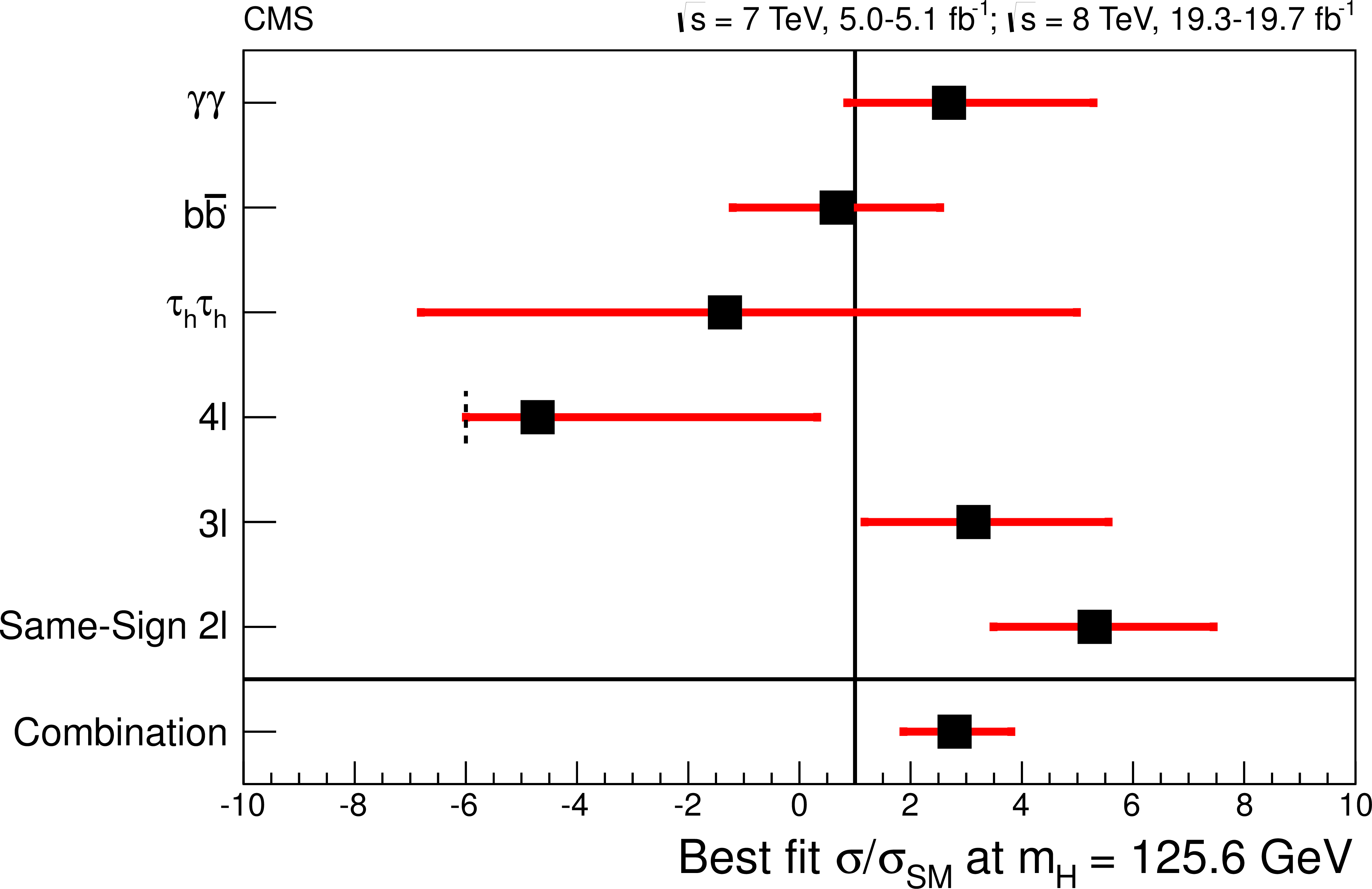
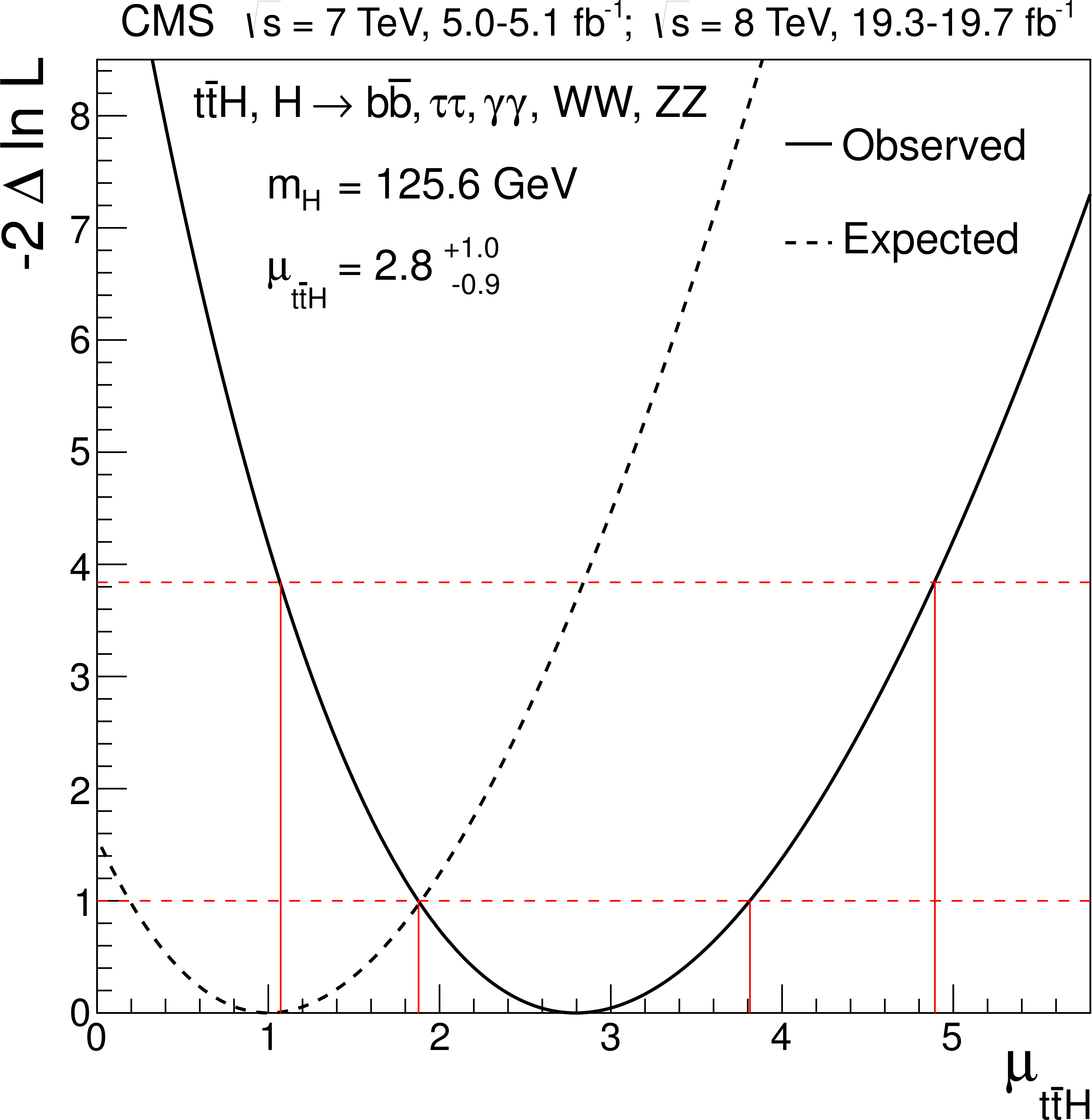
Figure 13-a:
Left: The best-fit values of the signal strength parameter $\mu = \sigma /\sigma _{\mathrm {SM}}$ for each $ { {\mathrm {t}\overline {\mathrm {t}}} {\mathrm {H}} } $ channel at $m_{ {\mathrm {H}} }$ = 125.6 GeV . The signal strength in the four-lepton final state is not allowed to be below approximately $-6$ by the requirement that the expected signal-plus-background event yield must not be negative in either of the two jet multiplicity bins. Right: The 1D test statistic $q$( $ {\mu _{ { {\mathrm {t}\overline {\mathrm {t}}} {\mathrm {H}} } }} $ ) scan vs. the signal strength parameter for $ { {\mathrm {t}\overline {\mathrm {t}}} {\mathrm {H}} } $ processes $ {\mu _{ { {\mathrm {t}\overline {\mathrm {t}}} {\mathrm {H}} } }} $, profiling all other nuisance parameters. The lower and upper horizontal lines correspond to the 68% and 95% CL, respectively. The $ {\mu _{ { {\mathrm {t}\overline {\mathrm {t}}} {\mathrm {H}} } }} $ values where these lines intersect with the $q$($ {\mu _{ { {\mathrm {t}\overline {\mathrm {t}}} {\mathrm {H}} } }} $) curve are shown by the vertical lines. |
png pdf |
Figure 13-b:
Left: The best-fit values of the signal strength parameter $\mu = \sigma /\sigma _{\mathrm {SM}}$ for each $ { {\mathrm {t}\overline {\mathrm {t}}} {\mathrm {H}} } $ channel at $m_{ {\mathrm {H}} }$ = 125.6 GeV . The signal strength in the four-lepton final state is not allowed to be below approximately $-6$ by the requirement that the expected signal-plus-background event yield must not be negative in either of the two jet multiplicity bins. Right: The 1D test statistic $q$( $ {\mu _{ { {\mathrm {t}\overline {\mathrm {t}}} {\mathrm {H}} } }} $ ) scan vs. the signal strength parameter for $ { {\mathrm {t}\overline {\mathrm {t}}} {\mathrm {H}} } $ processes $ {\mu _{ { {\mathrm {t}\overline {\mathrm {t}}} {\mathrm {H}} } }} $, profiling all other nuisance parameters. The lower and upper horizontal lines correspond to the 68% and 95% CL, respectively. The $ {\mu _{ { {\mathrm {t}\overline {\mathrm {t}}} {\mathrm {H}} } }} $ values where these lines intersect with the $q$($ {\mu _{ { {\mathrm {t}\overline {\mathrm {t}}} {\mathrm {H}} } }} $) curve are shown by the vertical lines. |
png pdf |
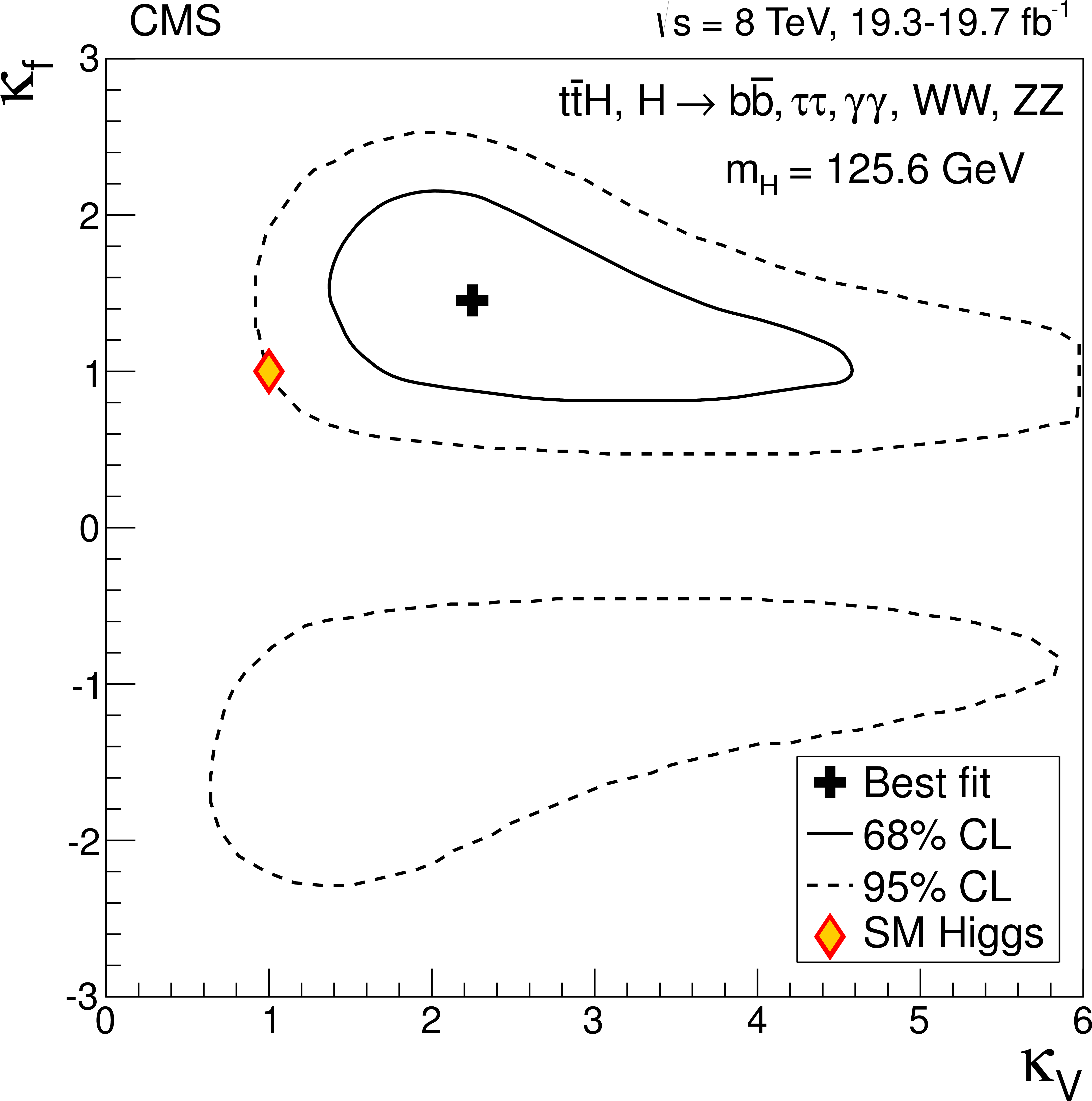
Figure 14:
The 2D test statistic $q$($ {\kappa _{\mathrm {V}}} $, $ {\kappa _{\mathrm {f}}} $) scan vs. the modifiers to the coupling of the Higgs boson to vector bosons ($ {\kappa _{\mathrm {V}}} $) and fermions ($ {\kappa _{\mathrm {f}}} $), profiling all other nuisances, extracted using only the $ {\mathrm {t}\overline {\mathrm {t}}} {\mathrm {H}} $ analysis channels. The contour lines at 68% CL (solid line) and 95% CL (dashed line) are shown. The best-fit and SM predicted values of the coupling modifiers ($ {\kappa _{\mathrm {V}}} $, $ {\kappa _{\mathrm {f}}} $) are given by the black cross and the open diamond, respectively. |
png pdf |
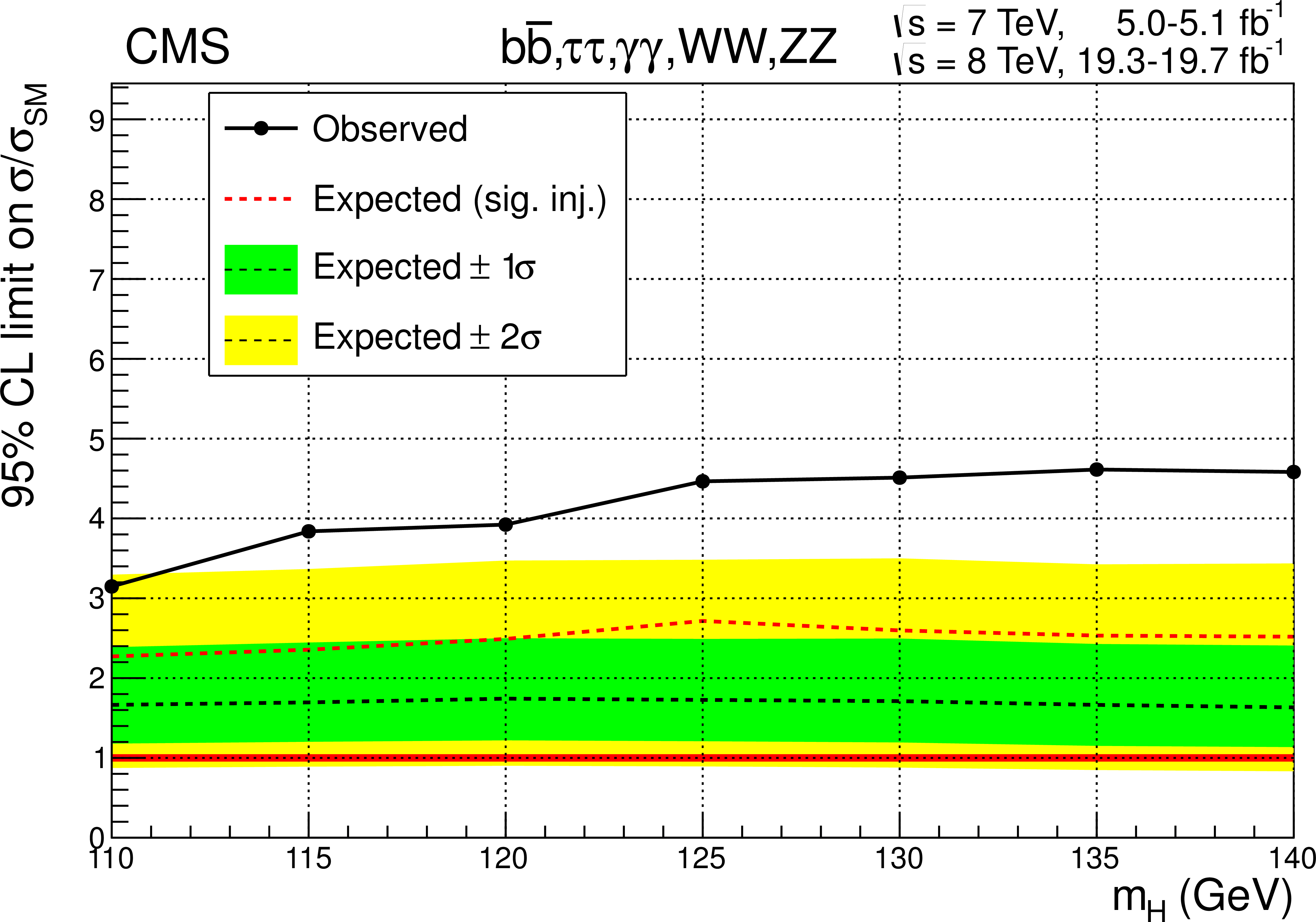
Figure 15-a:
The 95% CL upper limits on the signal strength parameter $\mu = \sigma /\sigma _{\mathrm {SM}}$. The black solid and dotted lines show the observed and background-only expected limits, respectively. The red dotted line shows the median expected limit for the SM Higgs boson with $m_{ {\mathrm {H}} }$ = 125.6 GeV . The green and yellow areas show the $1\sigma $ and $2\sigma $ bands, respectively. Left: limits as a function of $m_{ {\mathrm {H}} }$ for all channels combined. Right: limits for each channel at $m_{ {\mathrm {H}} }$ = 125.6 GeV . |

png pdf |
Figure 15-b:
The 95% CL upper limits on the signal strength parameter $\mu = \sigma /\sigma _{\mathrm {SM}}$. The black solid and dotted lines show the observed and background-only expected limits, respectively. The red dotted line shows the median expected limit for the SM Higgs boson with $m_{ {\mathrm {H}} }$ = 125.6 GeV . The green and yellow areas show the $1\sigma $ and $2\sigma $ bands, respectively. Left: limits as a function of $m_{ {\mathrm {H}} }$ for all channels combined. Right: limits for each channel at $m_{ {\mathrm {H}} }$ = 125.6 GeV . |
| Tables | |
png pdf |
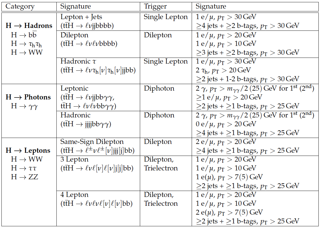
Table 1:
Summary of the search channels used in the $ {\mathrm {t}\overline {\mathrm {t}}} {\mathrm {H}} $ analysis. In the description of the signatures, an $\ell $ refers to any electron or muon in the final state (including those coming from leptonic $ {\tau }$ decays). A hadronic $ {\tau }$ decay is indicated by $ {\tau _\mathrm {h}} $. Finally, $\mathrm {j}$ represents a jet coming from any quark or gluon, or an unidentified hadronic $ {\tau }$ decay, while $ {\mathrm {b}}$ represents a b-quark jet. Any element in the signature enclosed in square brackets indicates that the element may not be present, depending on the specific decay mode of the top quark or Higgs boson. The minimum transverse momentum $ {p_{\mathrm {T}}} $ of various objects is given to convey some sense of the acceptance of each search channel; however, additional requirements are also applied. Jets labeled as b-tagged jets have been selected using the algorithm described in section 4. More details on the triggers used to collect data for each search channel are given in section 3. Selection of final-state objects (leptons, photons, jets, etc.) is described in general in section 4, with further channel-specific details included in sections 5-7. In this table and the rest of the paper, the number of b-tagged jets is always included in the jet count. For example, the notation 4jets + 2b-tags means four jets of which two jets are b-tagged. |
png pdf |
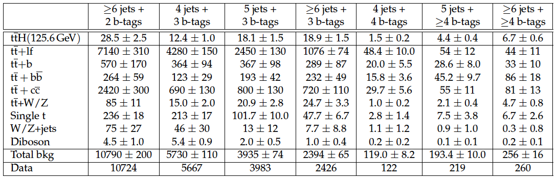
Table 2:
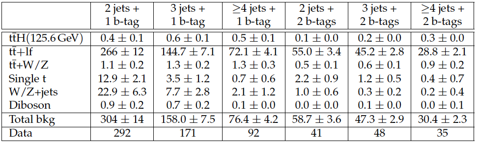
Expected event yields for signal ($m_{ {\mathrm {H}} } = $ 125.6 GeV) and backgrounds in the lepton+jets channel. Signal and background normalizations used for this table are described in the text. |

png pdf |
Table 3:
Expected event yields for signal ($m_{ {\mathrm {H}} } =$ 125.6 GeV) and backgrounds in the dilepton channel. Signal and background normalizations used for this table are described in the text. |
png pdf |
Table 4:
Expected event yields for signal ($m_{ {\mathrm {H}} } =$ 125.6 GeV) and backgrounds in the $ {\tau _\mathrm {h}} $ channel. Signal and background normalizations used for this table are described in the text. |
png pdf |
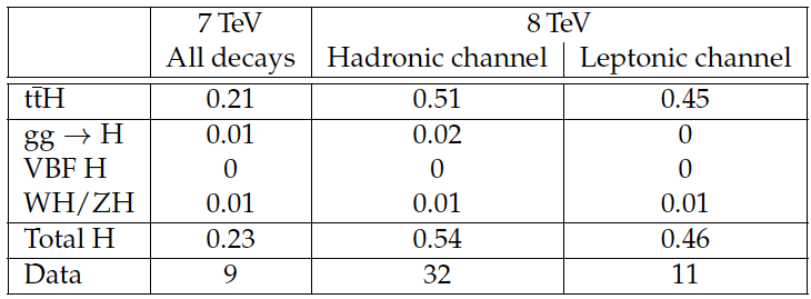
Table 5:
Expected signal yields after event selections in the 100 $ |
png pdf |
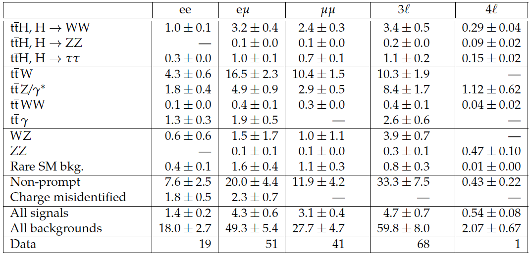
Table 6:
Expected and observed yields after the selection in all five final states. For the expected yields, the total systematic uncertainty is also indicated. The rare SM backgrounds include triboson production, $\mathrm {tbZ}$, $ {\mathrm {W}}^\pm {\mathrm {W}}^\pm \mathrm {qq}$, and $ {\mathrm {W}} {\mathrm {W}}$ produced in double parton interactions. A '-' indicates a negligible yield. Non-prompt and charge-misidentification backgrounds are described in section 7.3. |

png pdf |
Table 7:
Summary of systematic uncertainties. Each row in the table summarizes a category of systematic uncertainties from a common source or set of related sources. In the statistical implementation, most of these uncertainties are treated via multiple nuisance parameters. The table summarizes the impact of these uncertainties both in terms of the overall effect on signal and background rates, as well as on the shapes of the signal and background distributions. The rate columns show a range of uncertainties, since the size of the rate effect varies both with the analysis channel as well as the specific event selection category within a channel. The uncertainties quoted here are a priori uncertainties; that is they are calculated prior to fitting the data, which leads to a reduction in the impact of the uncertainties as the data helps to constrain them. |
png pdf |
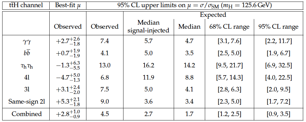
Table 8:
The best-fit values of the signal strength parameter $\mu = \sigma /\sigma _{\mathrm {SM}}$ for each $ { {\mathrm {t}\overline {\mathrm {t}}} {\mathrm {H}} } $ channel at $m_{ {\mathrm {H}} } =$ 125.6 GeV . The signal strength in the four-lepton final state is not allowed to be below approximately $-6$ by the requirement that the expected signal-plus-background event yield must not be negative in either of the two jet multiplicity bins. The observed and expected 95% CL upper limits on the signal strength parameter $\mu = \sigma /\sigma _{\mathrm {SM}}$ for each $ { {\mathrm {t}\overline {\mathrm {t}}} {\mathrm {H}} } $ channel at $m_{ {\mathrm {H}} } =$ 125.6 GeV are also shown. |
| Summary |
| The production of the standard model Higgs boson in association with a top-quark pair has been investigated using data recorded by the CMS experiment in 2011 and 2012, corresponding to integrated luminosities of up to 5.1 fb$^{-1}$ and 19.7 fb$^{-1}$ at $\sqrt{s} =$ 7 TeV and 8 TeV respectively. Signatures resulting from different combinations of decay modes for the top-quark pair and the Higgs boson have been analyzed. In particular, the searches have been optimized for the $\mathrm{ H \to b \overline{b} }$, $\mathrm{ \tau_h \tau_h }$, $\gamma \gamma $, $\mathrm{ WW }$, and $\mathrm{ ZZ }$ decay modes. The best-fit value for the signal strength $\mu$ is 2.8 $\pm$ 1.0 at 68% confidence level. This result represents an excess above the background- only expectation of 3.4 standard deviations. Compared to the SM expectation including the contribution from ttH, the observed excess is equivalent to a 2-standard-deviation upward fluctuation. These results are obtained assuming a Higgs boson mass of 125.6 GeV but they do not vary significantly for other choices of the mass in the vicinity of 125 GeV. These results are more consistent with the SM ttH expectation than with the background-only hypothesis. |
| Additional Figures | |
png pdf |
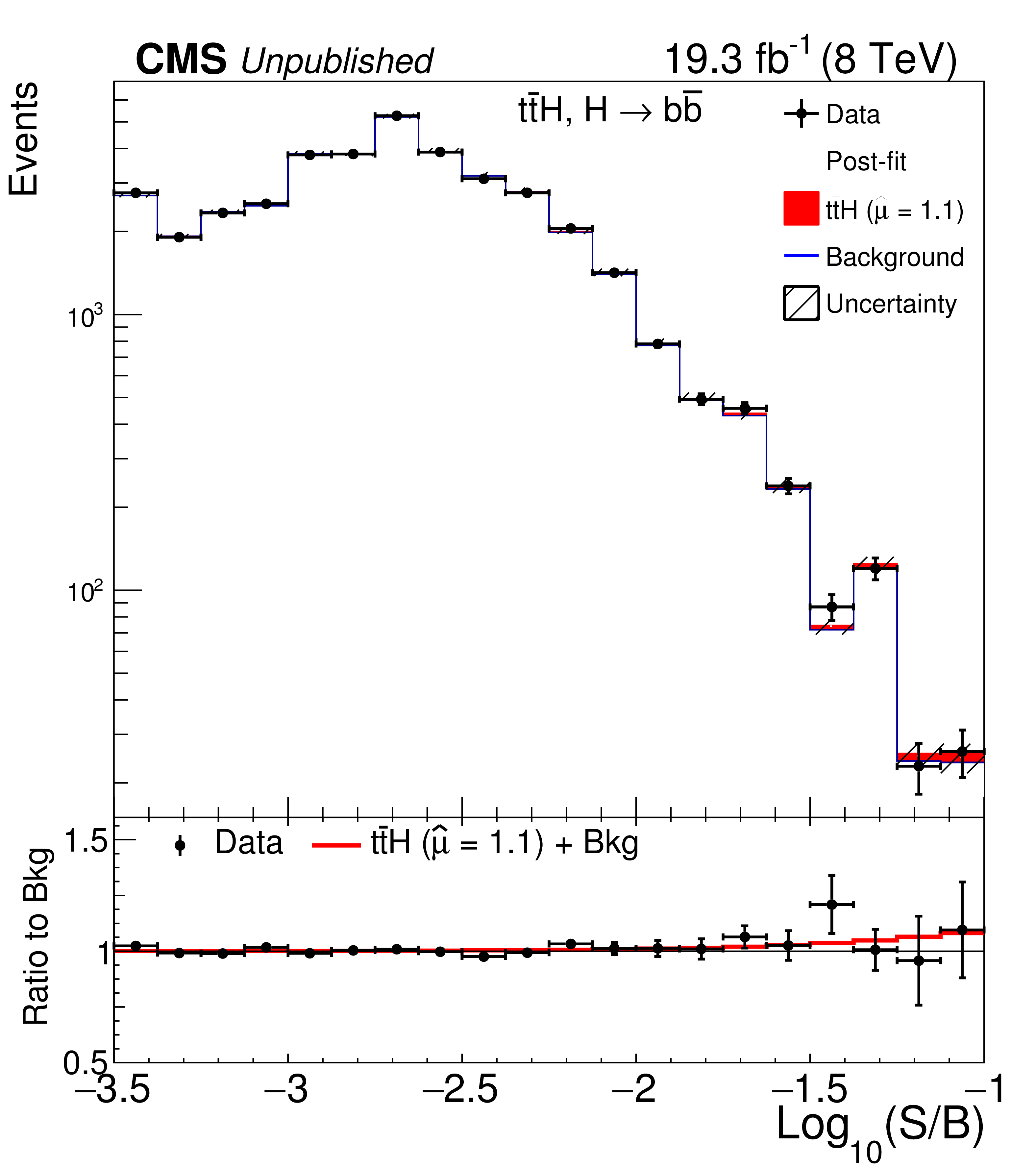
Additional Figure 1:
Yields of events in the $\mathrm{ t \overline{t} H } $ with $\mathrm{ H \to b \overline{b} } $ channel, ordered by the fraction of signal over background, using the best-fit nuisance parameter values for the backgrounds. |
|
|
Compact Muon Solenoid LHC, CERN |
|

|

|

|

|

|