

Compact Muon Solenoid
LHC, CERN
| CMS-HIG-13-032 ; CERN-EP-2016-050 | ||
| Search for two Higgs bosons in final states containing two photons and two bottom quarks | ||
| CMS Collaboration | ||
| 22 March 2016 | ||
| Phys. Rev. D 94 (2016) 052012 | ||
| Abstract: A search is presented for the production of two Higgs bosons in final states containing two photons and two bottom quarks. Both resonant and nonresonant hypotheses are investigated. The analyzed data correspond to an integrated luminosity of 19.7 fb$^{-1}$ of proton-proton collisions at $\sqrt{s} = $ 8 TeV collected with the CMS detector. Good agreement is observed between data and predictions of the standard model (SM). Upper limits are set at 95% confidence level on the production cross section of new particles and compared to the prediction for the existence of a warped extra dimension. When the decay to two Higgs bosons is kinematically allowed, assuming a mass scale $\Lambda_{\mathrm{R}} = $ 1 TeV for the model, the data exclude a radion scalar at masses below 980 GeV. The first Kaluza-Klein excitation mode of the graviton in Randall-Sundrum models is excluded for masses between 325 and 450 GeV. Limits set on nonresonant production constrain the parameter space for anomalous Higgs boson couplings. | ||
| Links: e-print arXiv:1603.06896 [hep-ex] (PDF) ; CDS record ; inSPIRE record ; HepData record ; CADI line (restricted) ; | ||
| Figures | |
png pdf |
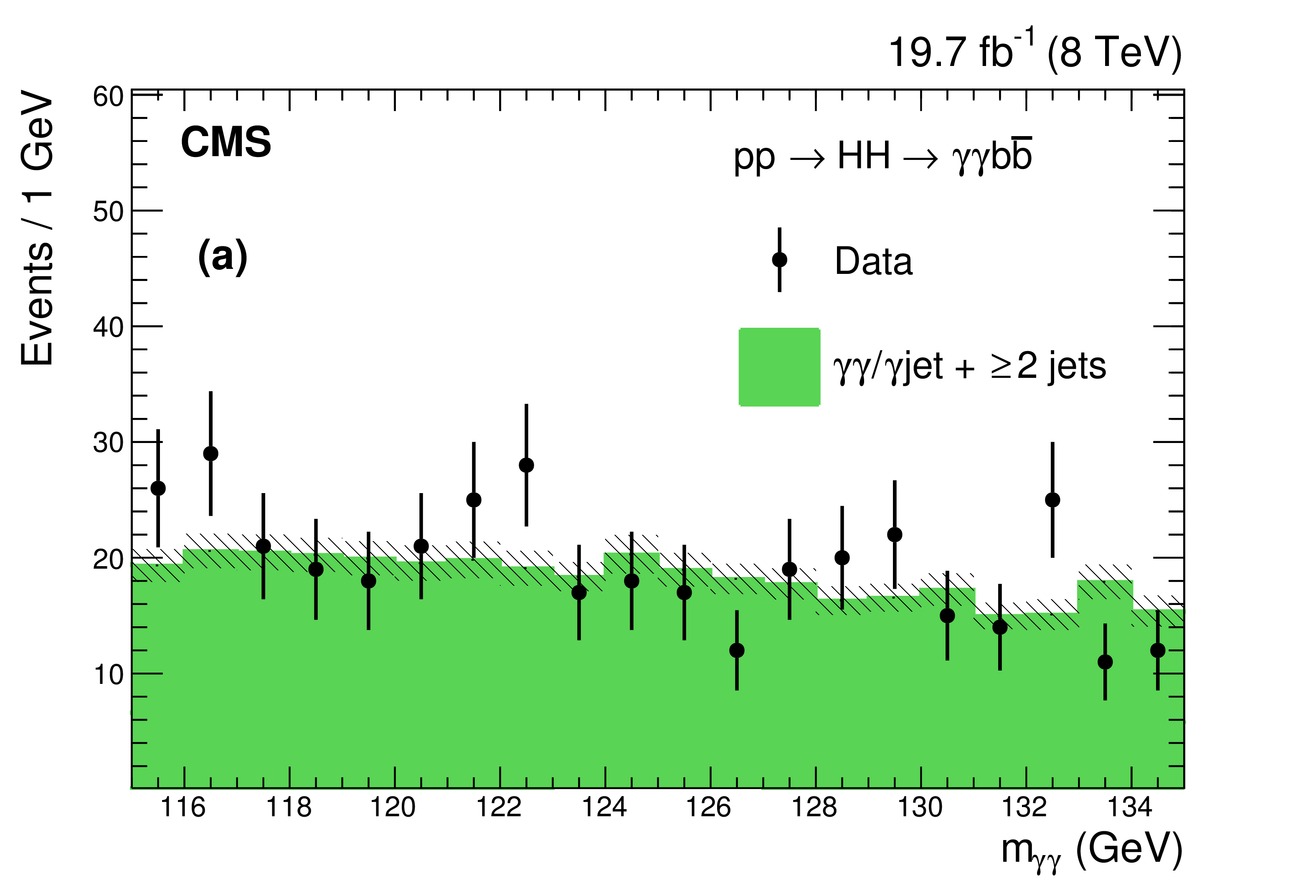
Figure 1-a:
Reconstructed spectra for data compared to the $\gamma \gamma /\gamma + \text {jet} + {\geq }2 \text {jets}$ background, after object selections on photons and jets and a requirement of at least one b-tagged jet: (a) $ {m_{\gamma \gamma }} $, (b) $ {m_\mathrm {jj}} $, (c) $ | \cos \theta^{\text{CS}}_{\mathrm{ H H } } | $, and (d) $ {m_{\gamma \gamma \mathrm {jj}}^\text {kin}} $. The hatched area corresponds to the bin-by-bin statistical uncertainties on the background prediction reflecting the limited size of the generated MC sample. The comparison is provided for illustrative purpose, in the analysis the backgrounds, except the one coming from single-Higgs production, are evaluated from a fit to the data without reference to the MC simulation. |
png pdf |
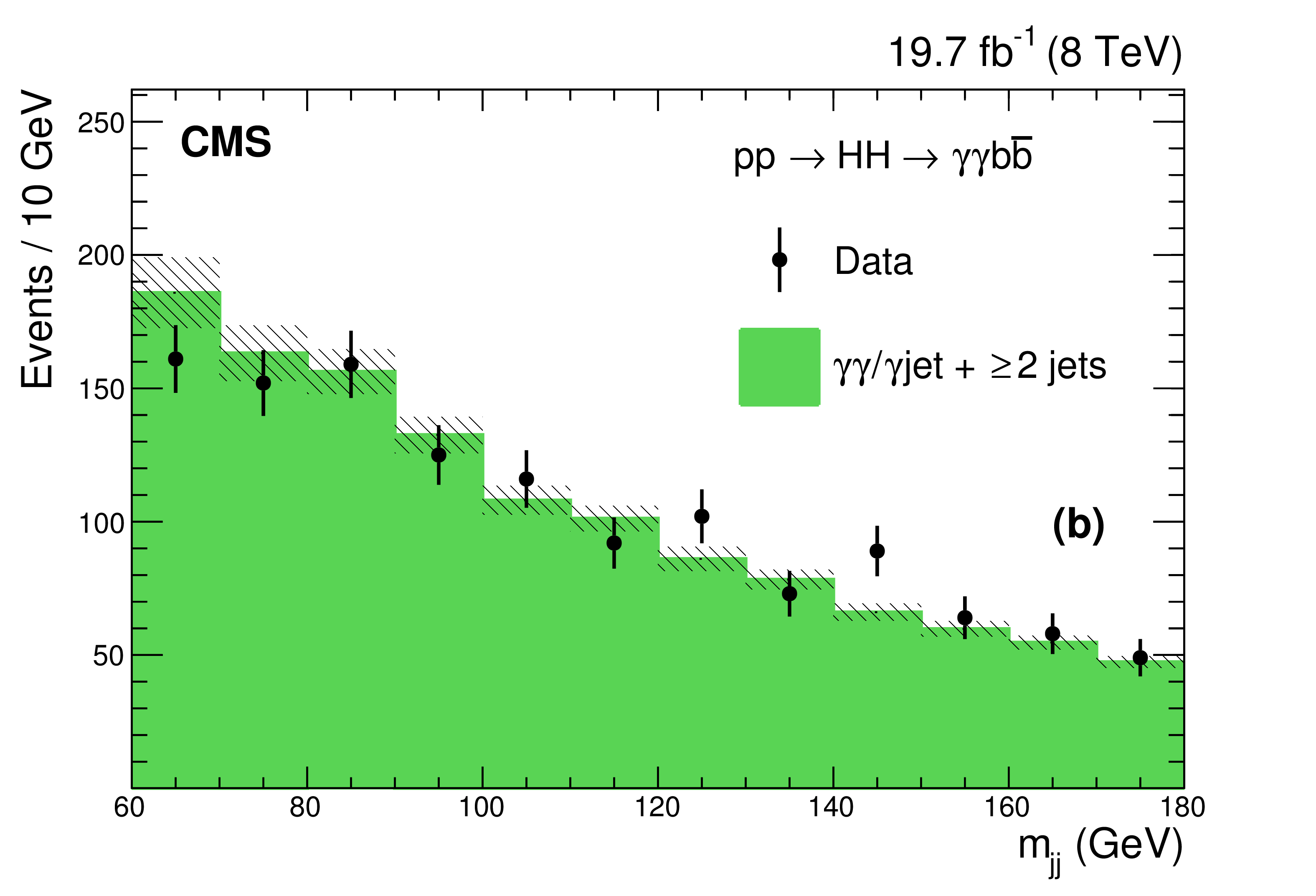
Figure 1-b:
Reconstructed spectra for data compared to the $\gamma \gamma /\gamma + \text {jet} + {\geq }2 \text {jets}$ background, after object selections on photons and jets and a requirement of at least one b-tagged jet: (a) $ {m_{\gamma \gamma }} $, (b) $ {m_\mathrm {jj}} $, (c) $ | \cos \theta^{\text{CS}}_{\mathrm{ H H } } | $, and (d) $ {m_{\gamma \gamma \mathrm {jj}}^\text {kin}} $. The hatched area corresponds to the bin-by-bin statistical uncertainties on the background prediction reflecting the limited size of the generated MC sample. The comparison is provided for illustrative purpose, in the analysis the backgrounds, except the one coming from single-Higgs production, are evaluated from a fit to the data without reference to the MC simulation. |
png pdf |
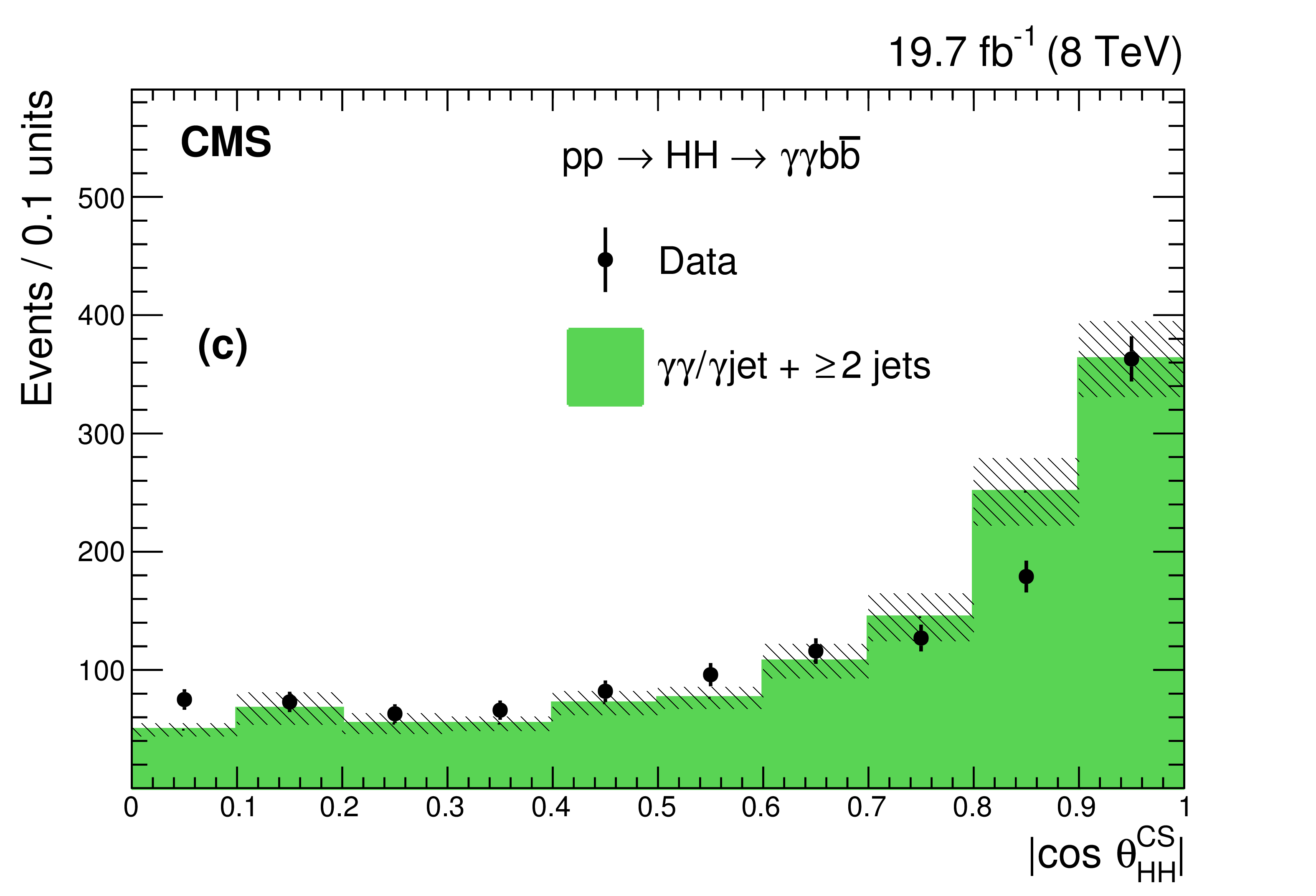
Figure 1-c:
Reconstructed spectra for data compared to the $\gamma \gamma /\gamma + \text {jet} + {\geq }2 \text {jets}$ background, after object selections on photons and jets and a requirement of at least one b-tagged jet: (a) $ {m_{\gamma \gamma }} $, (b) $ {m_\mathrm {jj}} $, (c) $ | \cos \theta^{\text{CS}}_{\mathrm{ H H } } | $, and (d) $ {m_{\gamma \gamma \mathrm {jj}}^\text {kin}} $. The hatched area corresponds to the bin-by-bin statistical uncertainties on the background prediction reflecting the limited size of the generated MC sample. The comparison is provided for illustrative purpose, in the analysis the backgrounds, except the one coming from single-Higgs production, are evaluated from a fit to the data without reference to the MC simulation. |
png pdf |
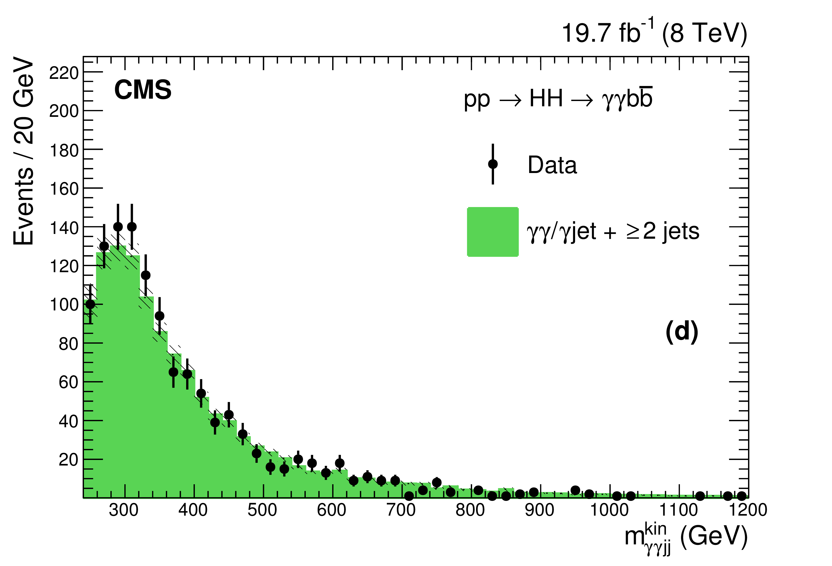
Figure 1-d:
Reconstructed spectra for data compared to the $\gamma \gamma /\gamma + \text {jet} + {\geq }2 \text {jets}$ background, after object selections on photons and jets and a requirement of at least one b-tagged jet: (a) $ {m_{\gamma \gamma }} $, (b) $ {m_\mathrm {jj}} $, (c) $ | \cos \theta^{\text{CS}}_{\mathrm{ H H } } | $, and (d) $ {m_{\gamma \gamma \mathrm {jj}}^\text {kin}} $. The hatched area corresponds to the bin-by-bin statistical uncertainties on the background prediction reflecting the limited size of the generated MC sample. The comparison is provided for illustrative purpose, in the analysis the backgrounds, except the one coming from single-Higgs production, are evaluated from a fit to the data without reference to the MC simulation. |
png pdf |
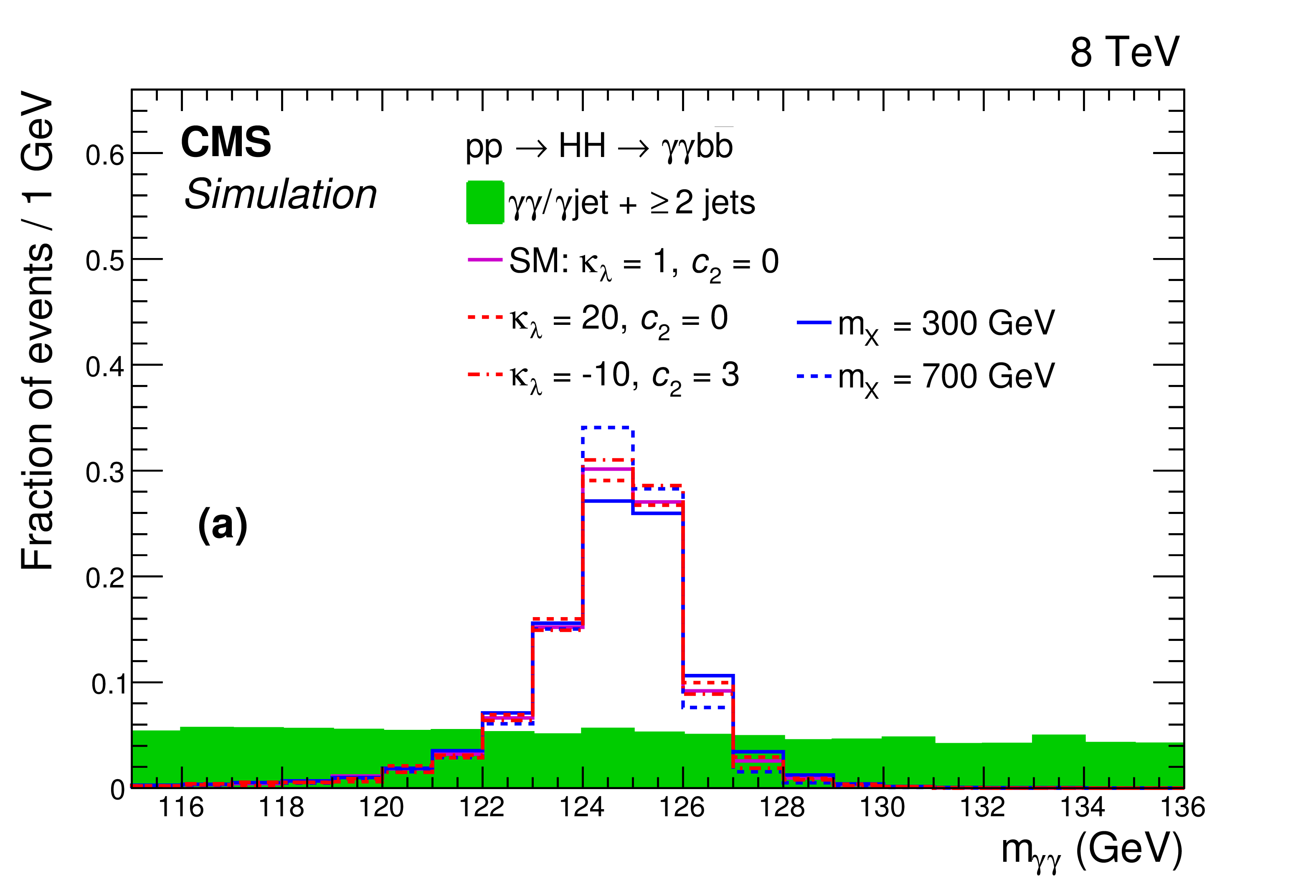
Figure 2-a:
Simulated spectra for the spin-0 radion signal at $ {m_\mathrm {X}} =$ 300 and 700 GeV, and for some values of the anomalous couplings, compared to SM Higgs boson production and QCD background, after object selections on photons and jets and a requirement of at least one b-tagged jet: (a) $ {m_{\gamma \gamma }} $, (b) $ {m_\mathrm {jj}} $, (c) $ | \cos \theta^{\text{CS}}_{\mathrm{ H H } } | $, and (d) $ {m_{\gamma \gamma \mathrm {jj}}^\text {kin}} $. All spectra are normalized to unity. |
png pdf |
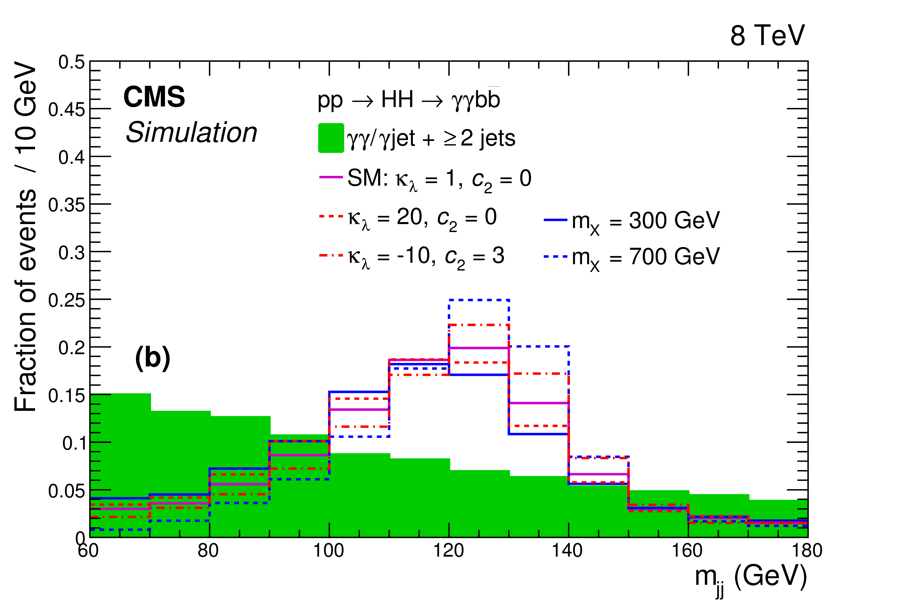
Figure 2-b:
Simulated spectra for the spin-0 radion signal at $ {m_\mathrm {X}} =$ 300 and 700 GeV, and for some values of the anomalous couplings, compared to SM Higgs boson production and QCD background, after object selections on photons and jets and a requirement of at least one b-tagged jet: (a) $ {m_{\gamma \gamma }} $, (b) $ {m_\mathrm {jj}} $, (c) $ | \cos \theta^{\text{CS}}_{\mathrm{ H H } } | $, and (d) $ {m_{\gamma \gamma \mathrm {jj}}^\text {kin}} $. All spectra are normalized to unity. |
png pdf |
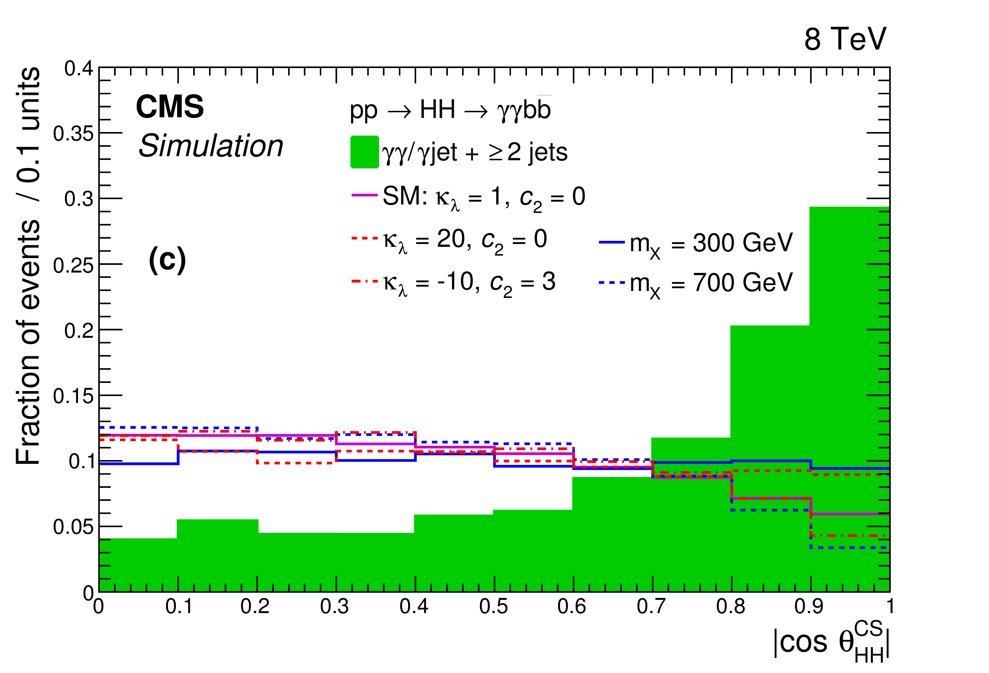
Figure 2-c:
Simulated spectra for the spin-0 radion signal at $ {m_\mathrm {X}} =$ 300 and 700 GeV, and for some values of the anomalous couplings, compared to SM Higgs boson production and QCD background, after object selections on photons and jets and a requirement of at least one b-tagged jet: (a) $ {m_{\gamma \gamma }} $, (b) $ {m_\mathrm {jj}} $, (c) $ | \cos \theta^{\text{CS}}_{\mathrm{ H H } } | $, and (d) $ {m_{\gamma \gamma \mathrm {jj}}^\text {kin}} $. All spectra are normalized to unity. |
png pdf |
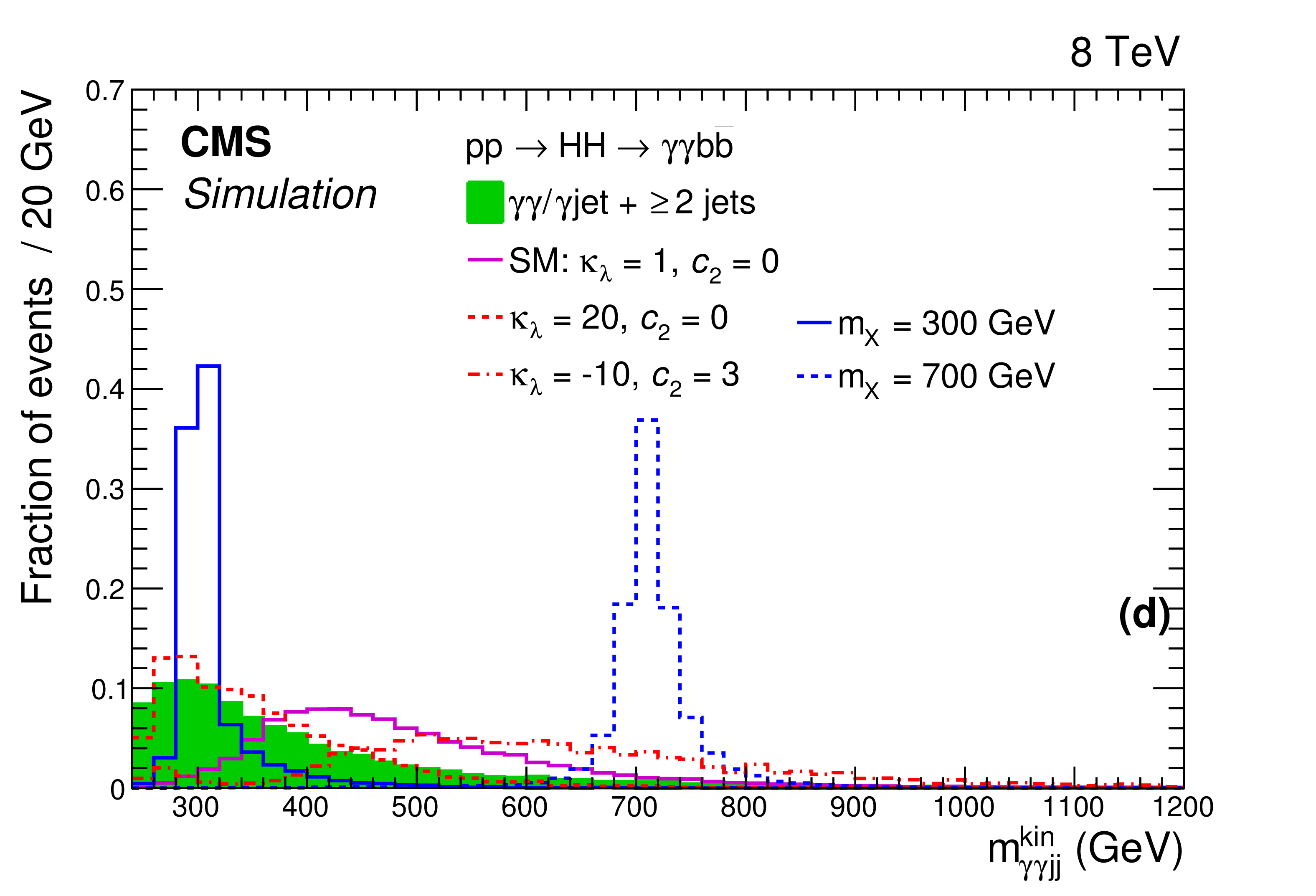
Figure 2-d:
Simulated spectra for the spin-0 radion signal at $ {m_\mathrm {X}} =$ 300 and 700 GeV, and for some values of the anomalous couplings, compared to SM Higgs boson production and QCD background, after object selections on photons and jets and a requirement of at least one b-tagged jet: (a) $ {m_{\gamma \gamma }} $, (b) $ {m_\mathrm {jj}} $, (c) $ | \cos \theta^{\text{CS}}_{\mathrm{ H H } } | $, and (d) $ {m_{\gamma \gamma \mathrm {jj}}^\text {kin}} $. All spectra are normalized to unity. |
png pdf |
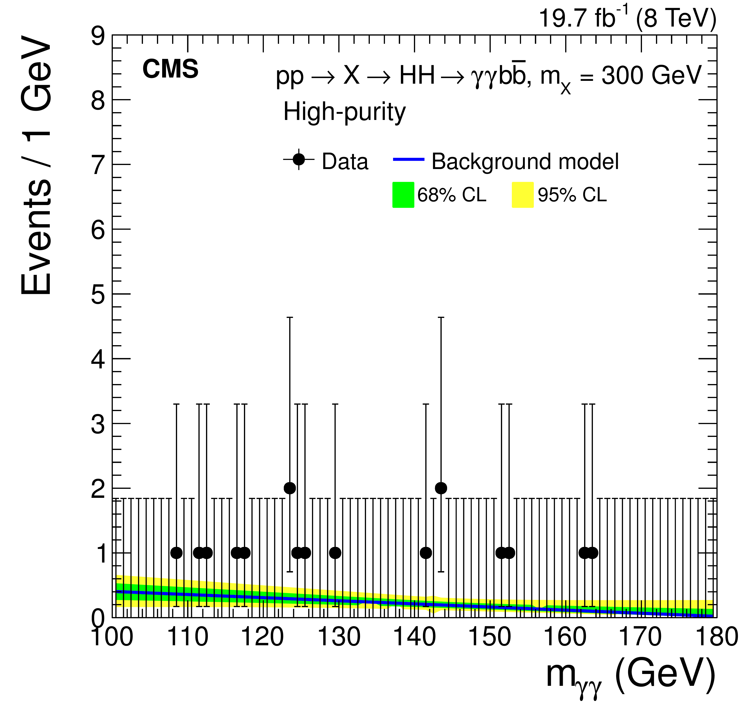
Figure 3-a:
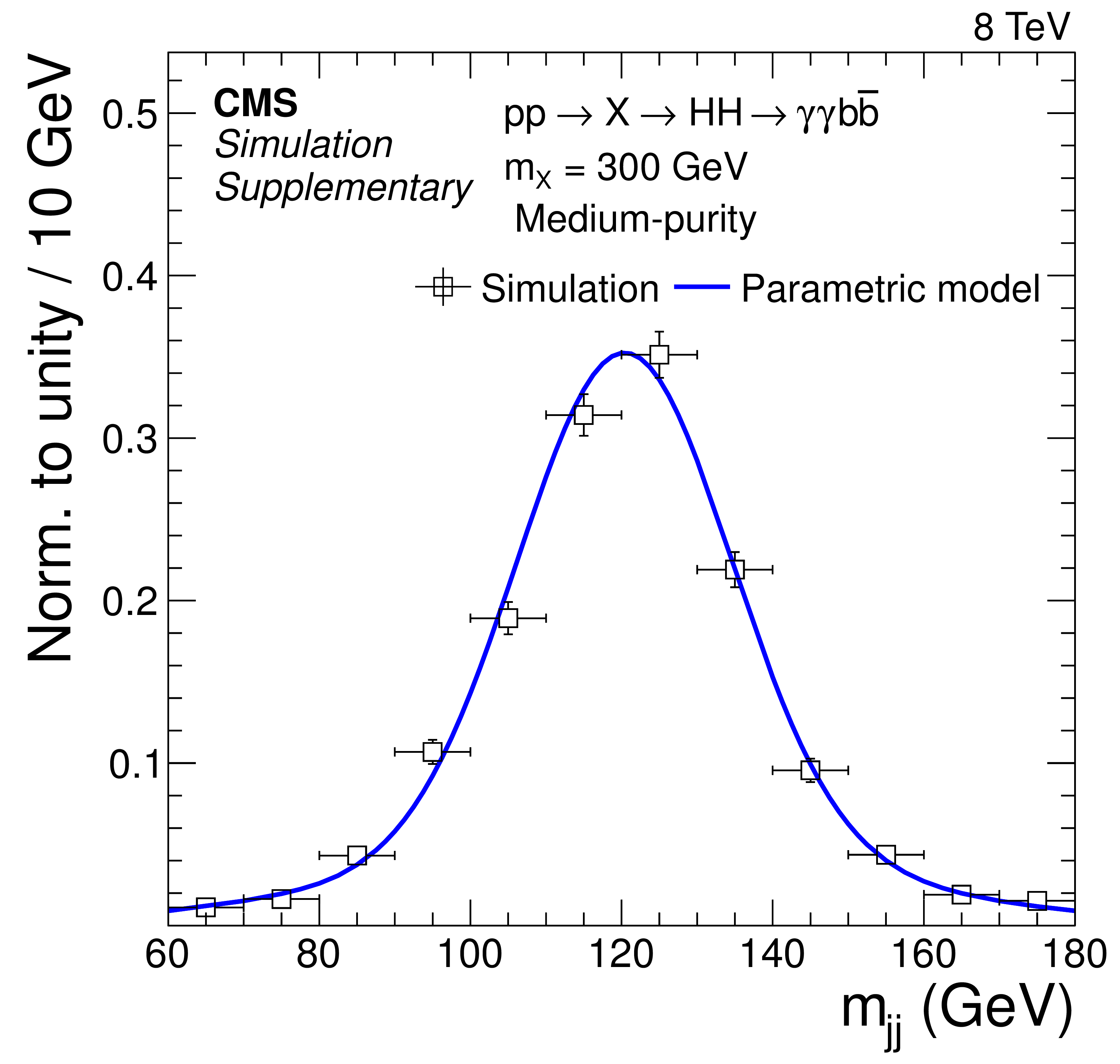
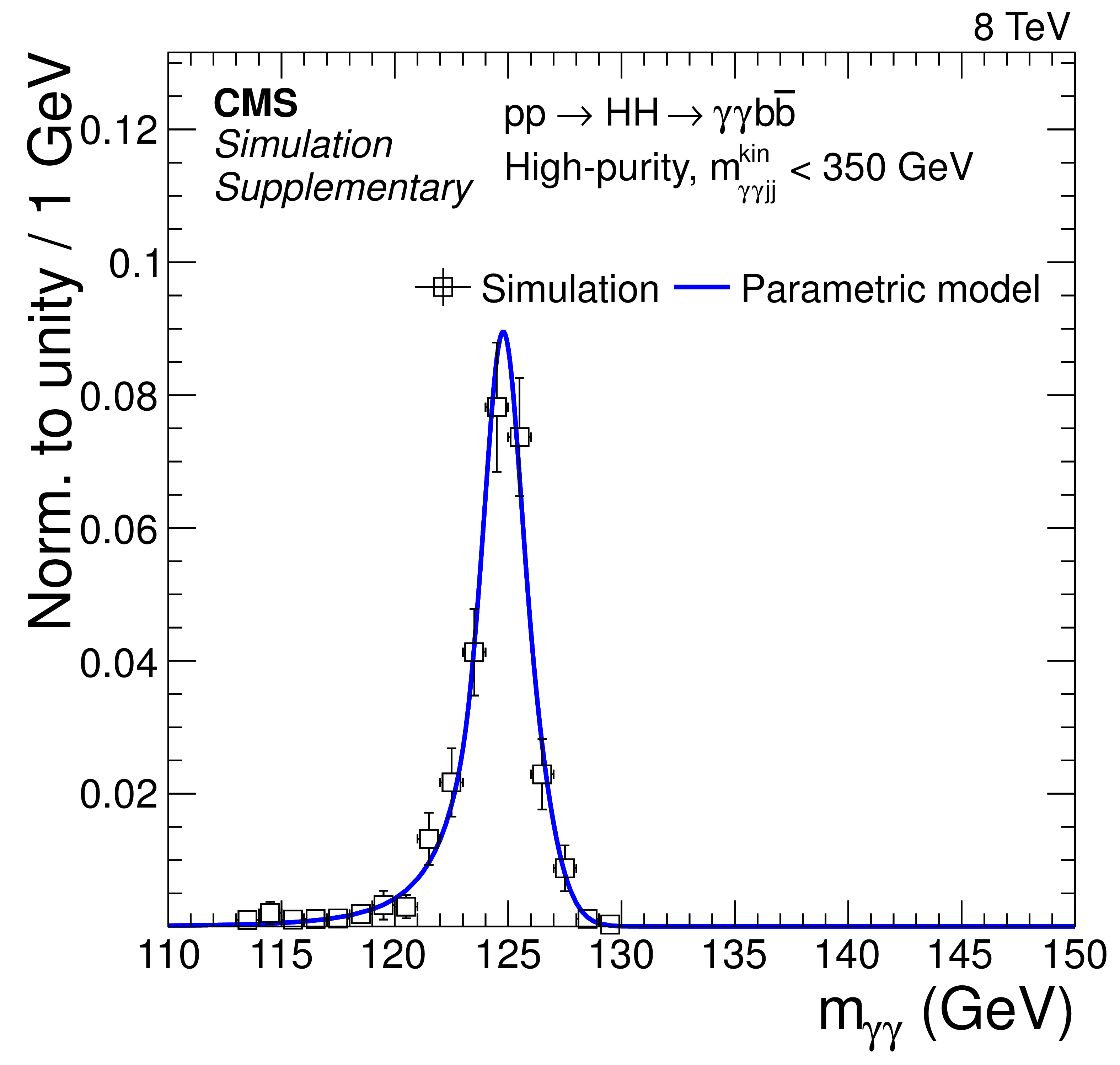
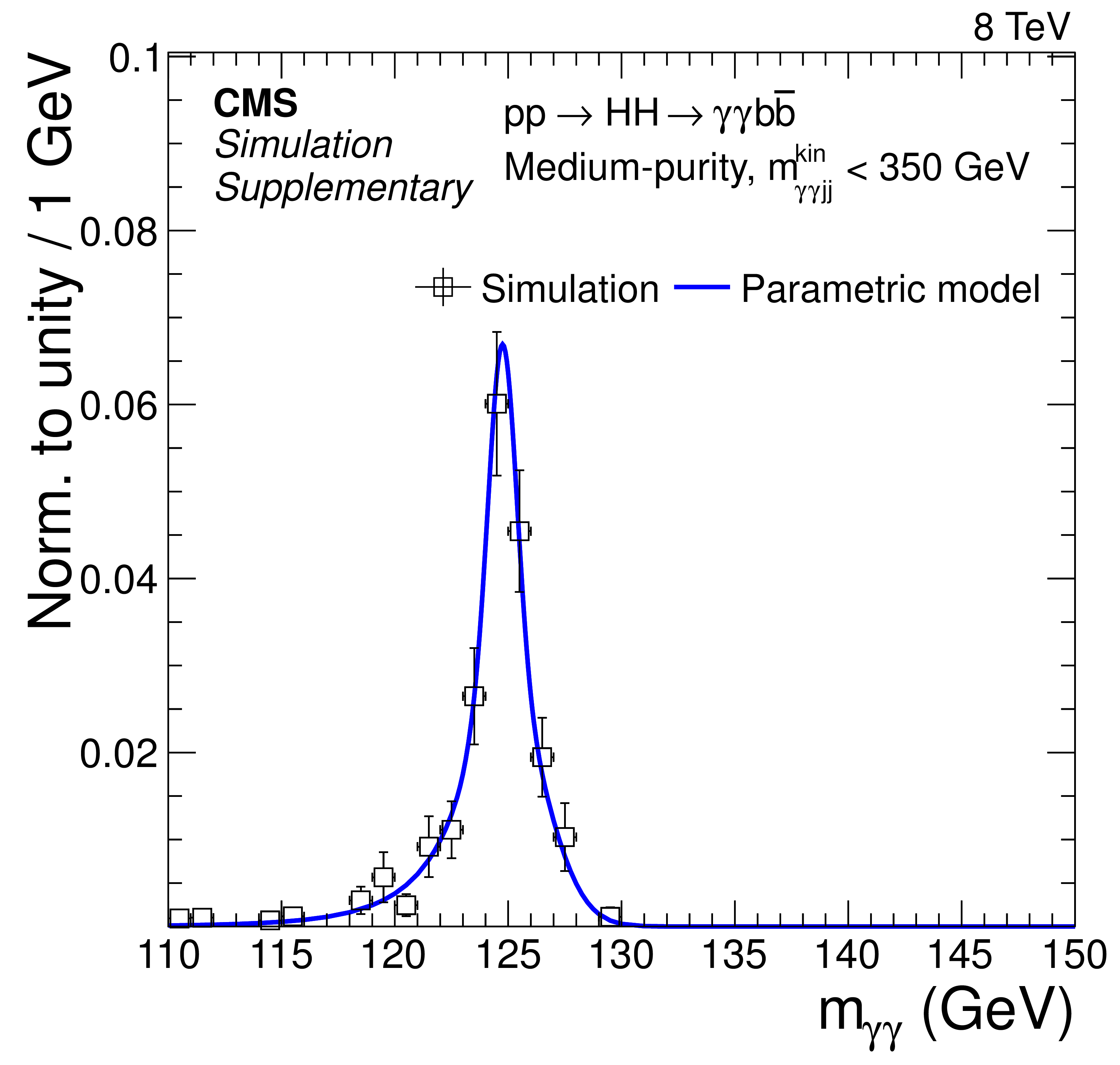
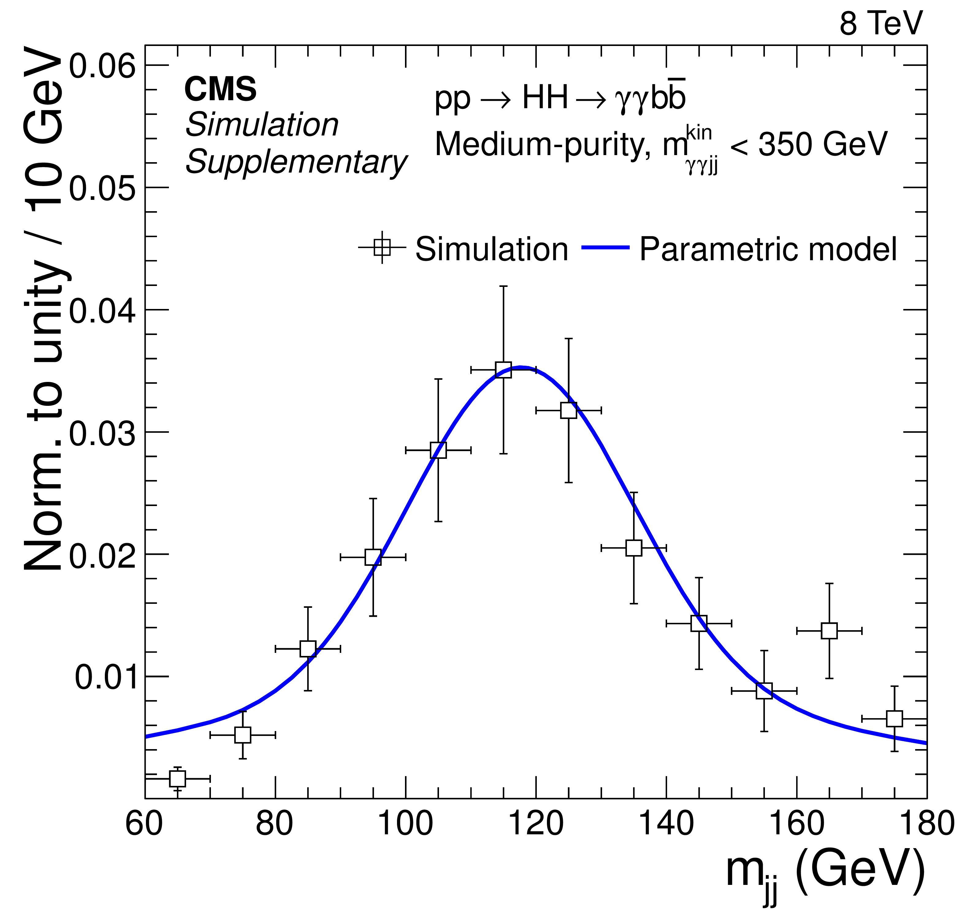
Fits to the nonresonant background contribution in high-purity category to the $ {m_{\gamma \gamma }} $ (top-left) and $ {m_\mathrm {jj}} $ spectra (top-right), and similarly for medium-purity category in bottom-left and bottom-right, respectively. The fits to the background-only hypothesis are given by the blue curves, along with their 68% and 95% CL contours. The selections are designed to search for a $ {m_\mathrm {X}} = $ 300 GeV hypothesis. |

png pdf |
Figure 3-b:
Fits to the nonresonant background contribution in high-purity category to the $ {m_{\gamma \gamma }} $ (top-left) and $ {m_\mathrm {jj}} $ spectra (top-right), and similarly for medium-purity category in bottom-left and bottom-right, respectively. The fits to the background-only hypothesis are given by the blue curves, along with their 68% and 95% CL contours. The selections are designed to search for a $ {m_\mathrm {X}} = $ 300 GeV hypothesis. |
png pdf |
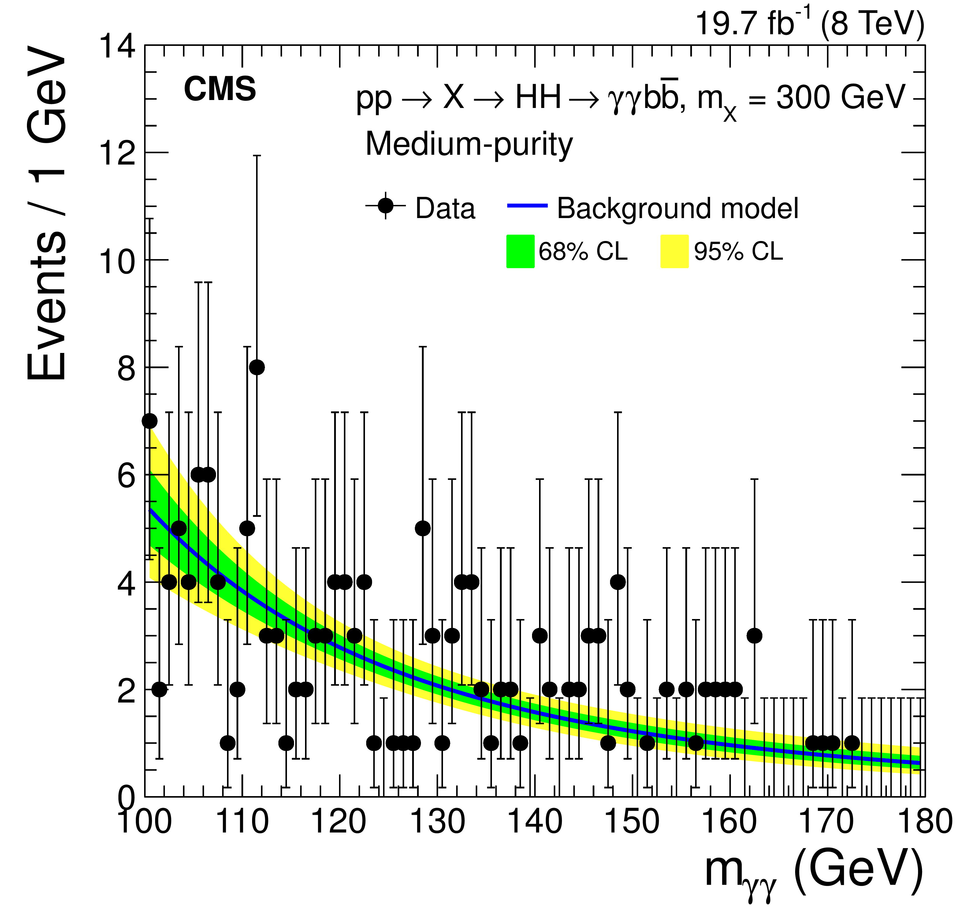
Figure 3-c:
Fits to the nonresonant background contribution in high-purity category to the $ {m_{\gamma \gamma }} $ (top-left) and $ {m_\mathrm {jj}} $ spectra (top-right), and similarly for medium-purity category in bottom-left and bottom-right, respectively. The fits to the background-only hypothesis are given by the blue curves, along with their 68% and 95% CL contours. The selections are designed to search for a $ {m_\mathrm {X}} = $ 300 GeV hypothesis. |
png pdf |
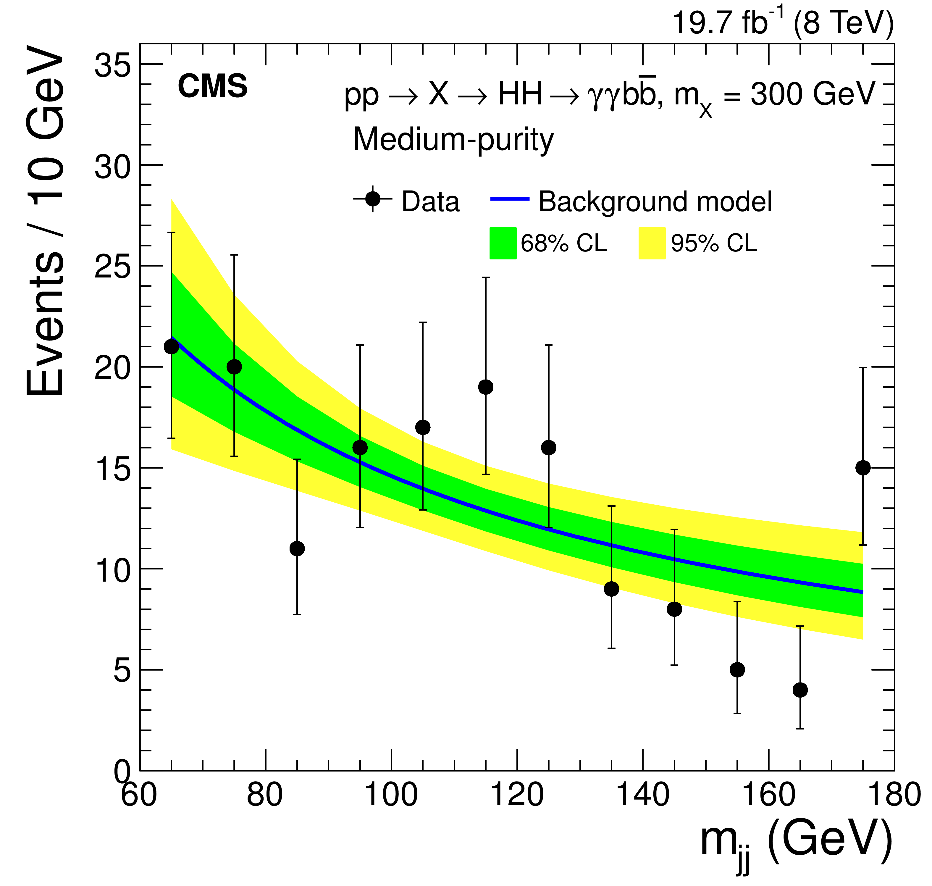
Figure 3-d:
Fits to the nonresonant background contribution in high-purity category to the $ {m_{\gamma \gamma }} $ (top-left) and $ {m_\mathrm {jj}} $ spectra (top-right), and similarly for medium-purity category in bottom-left and bottom-right, respectively. The fits to the background-only hypothesis are given by the blue curves, along with their 68% and 95% CL contours. The selections are designed to search for a $ {m_\mathrm {X}} = $ 300 GeV hypothesis. |
png pdf |
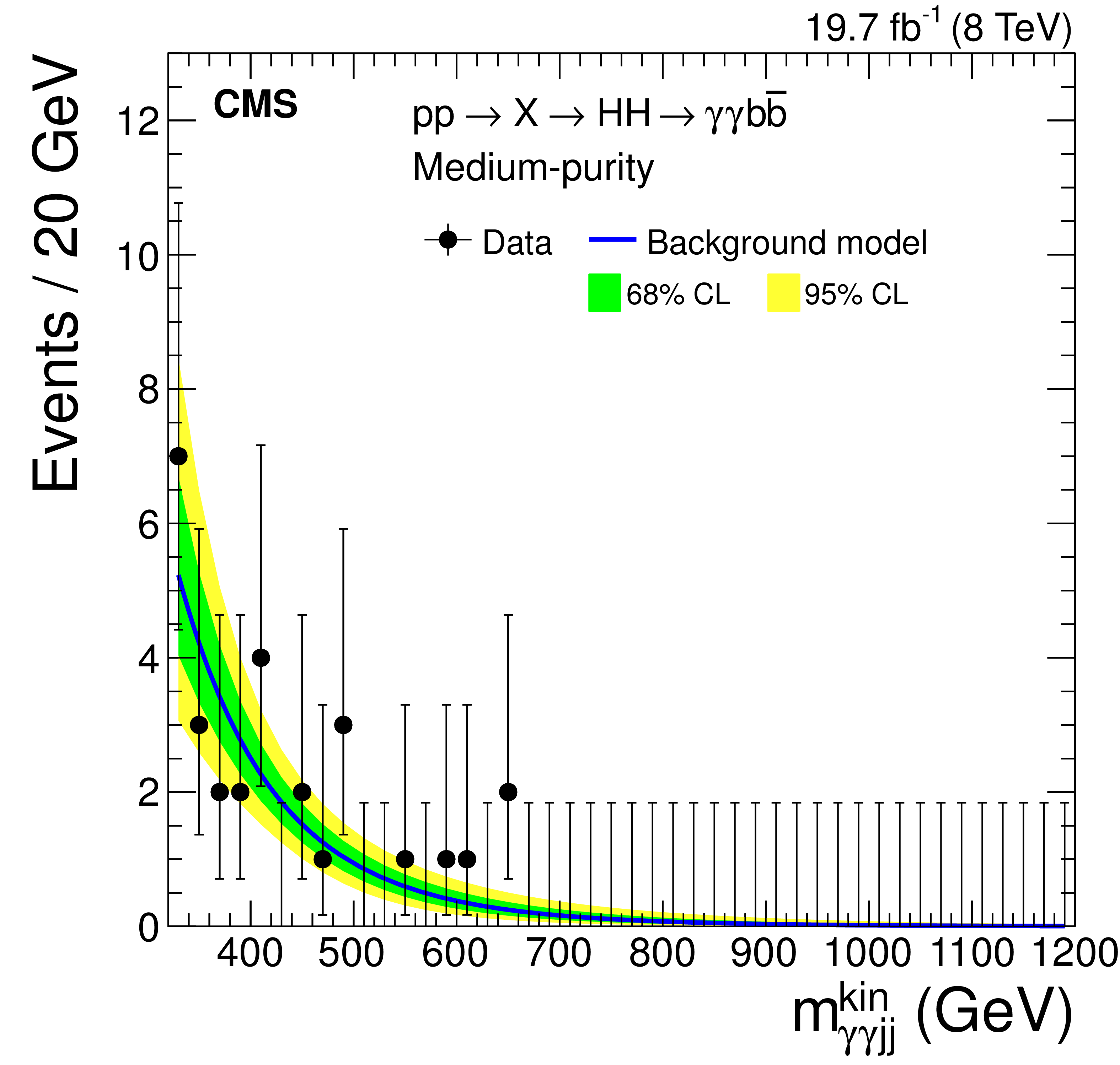
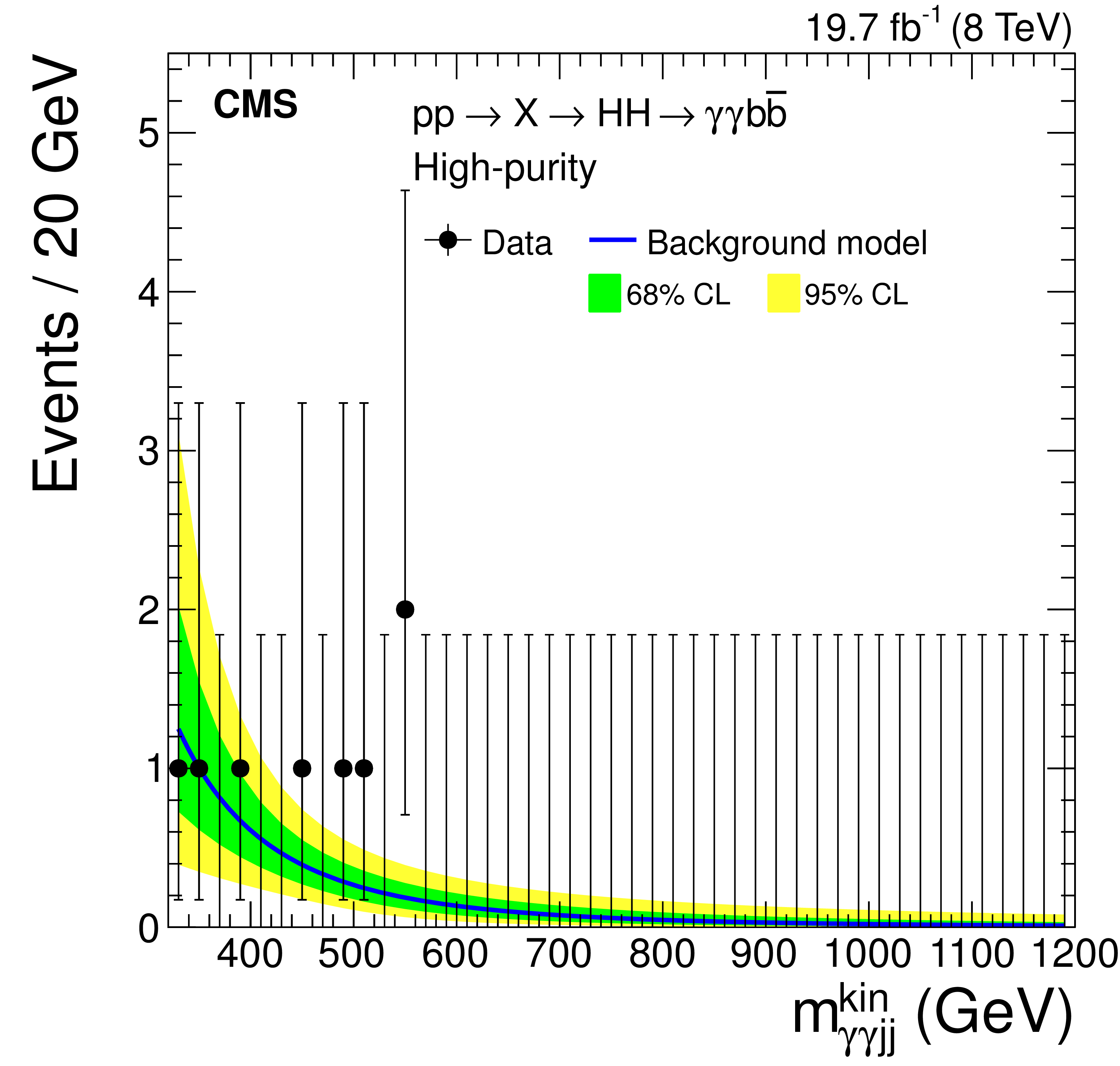
Figure 4-a:
Fits to the nonresonant background contribution to the $ {m_{\gamma \gamma \mathrm {jj}}^\text {kin}} $ spectrum in medium- (a) and in high-purity (b) events. The fits to the background-only hypothesis are given by the blue curves, along with their 68% and 95% CL contours. |
png pdf |
Figure 4-b:
Fits to the nonresonant background contribution to the $ {m_{\gamma \gamma \mathrm {jj}}^\text {kin}} $ spectrum in medium- (a) and in high-purity (b) events. The fits to the background-only hypothesis are given by the blue curves, along with their 68% and 95% CL contours. |
png pdf |
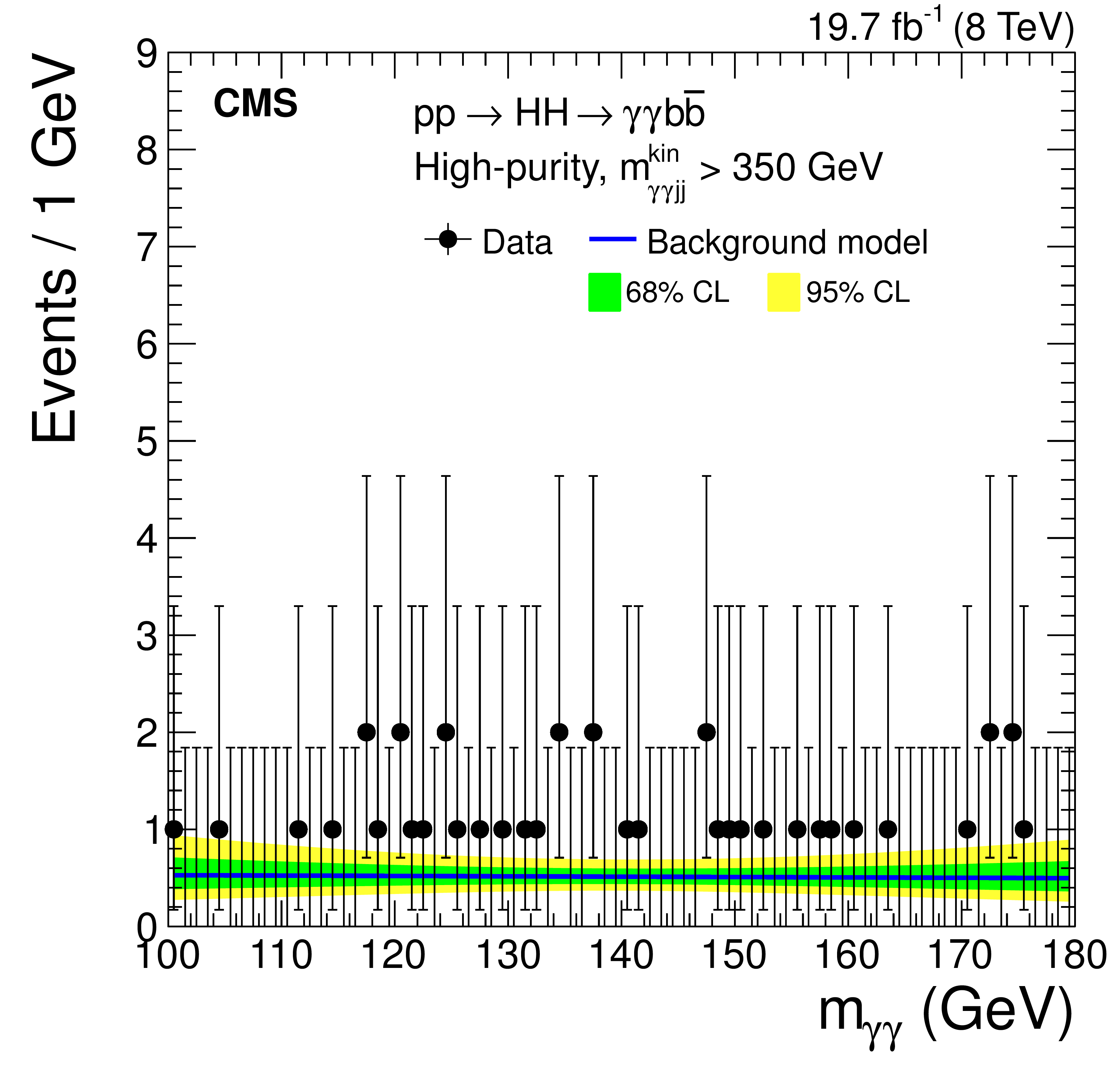
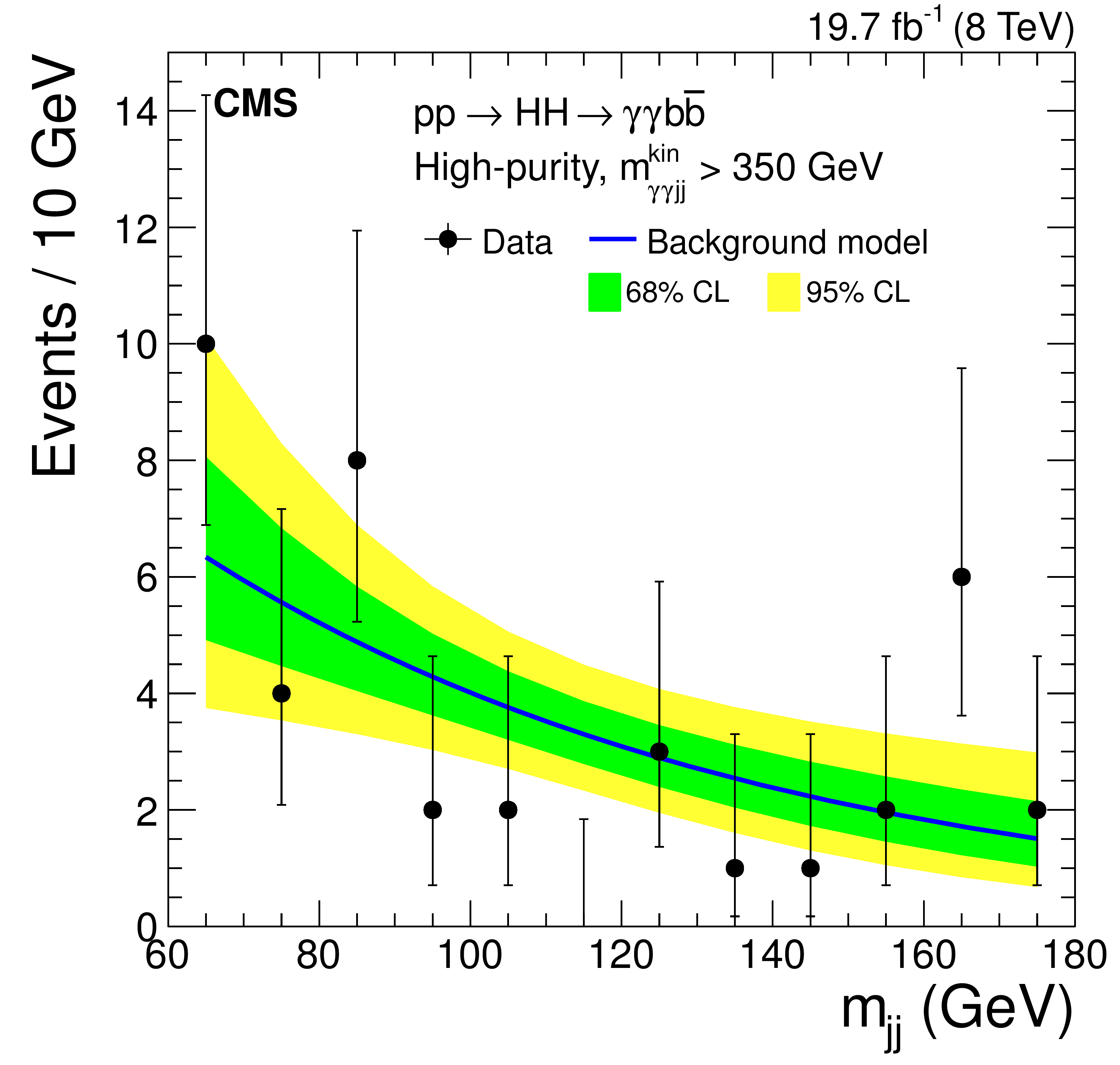
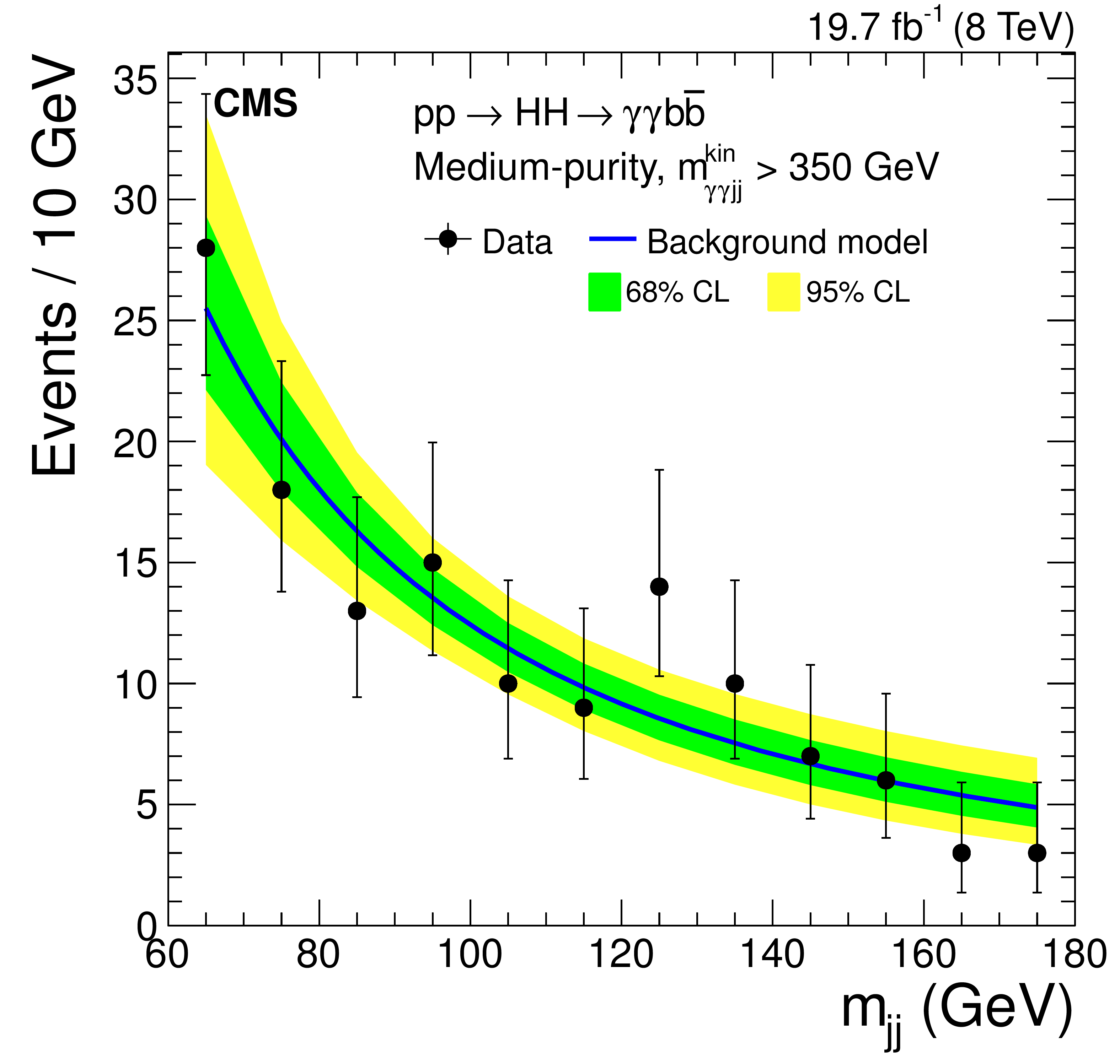
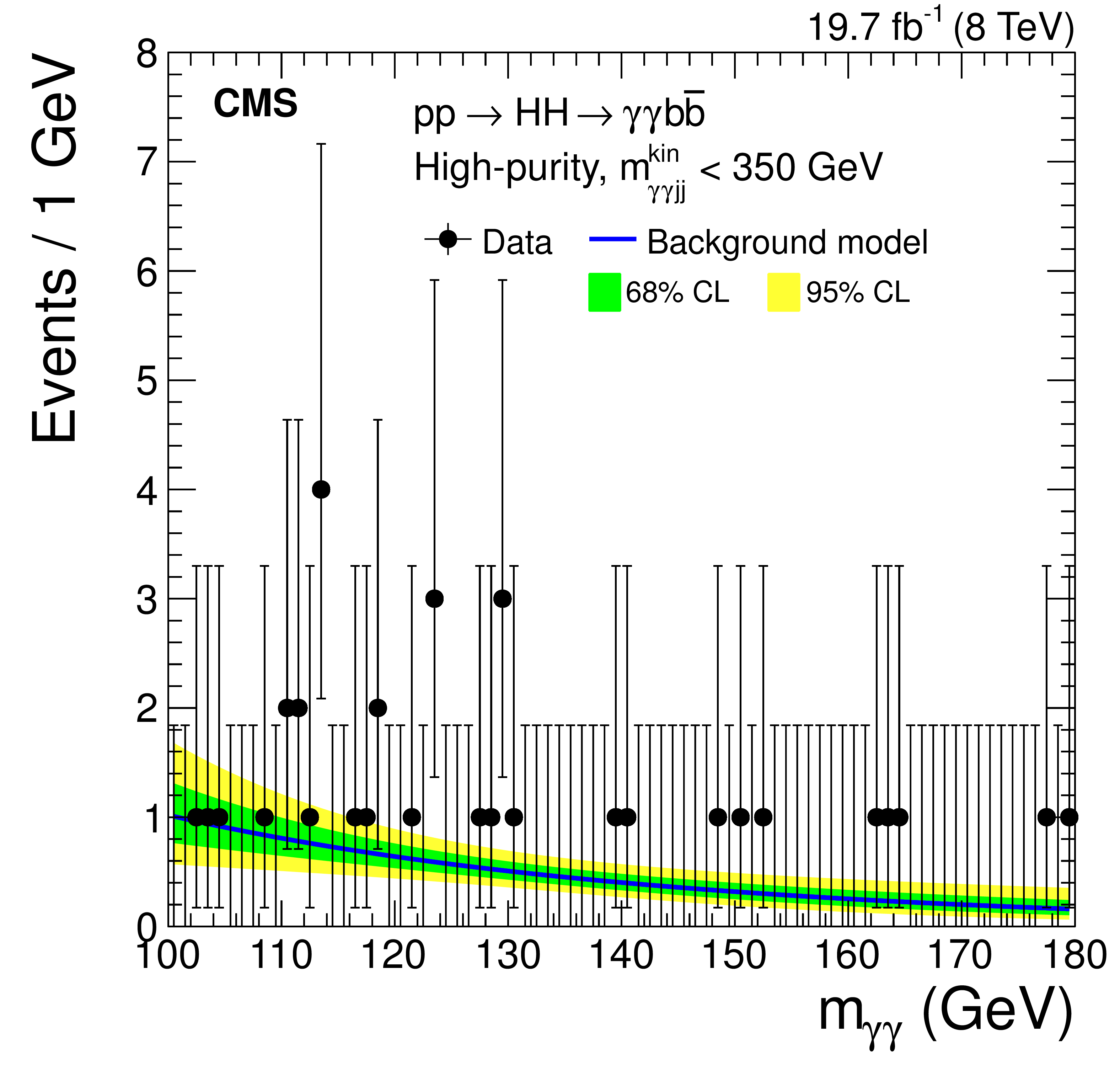
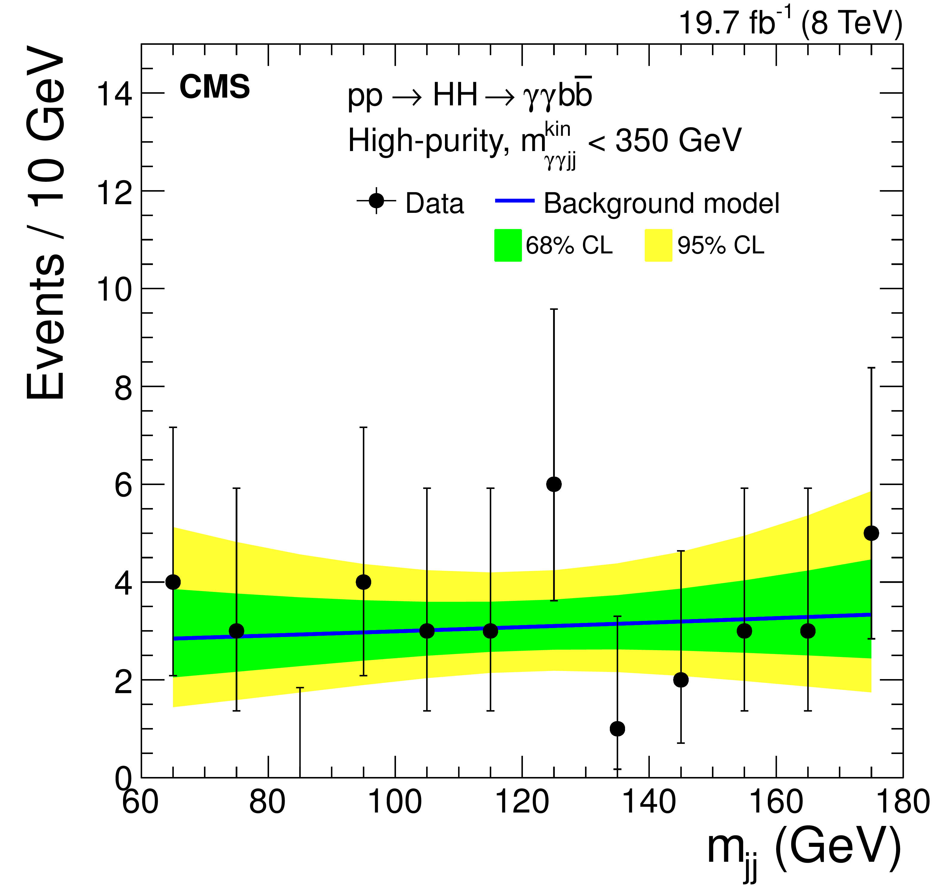
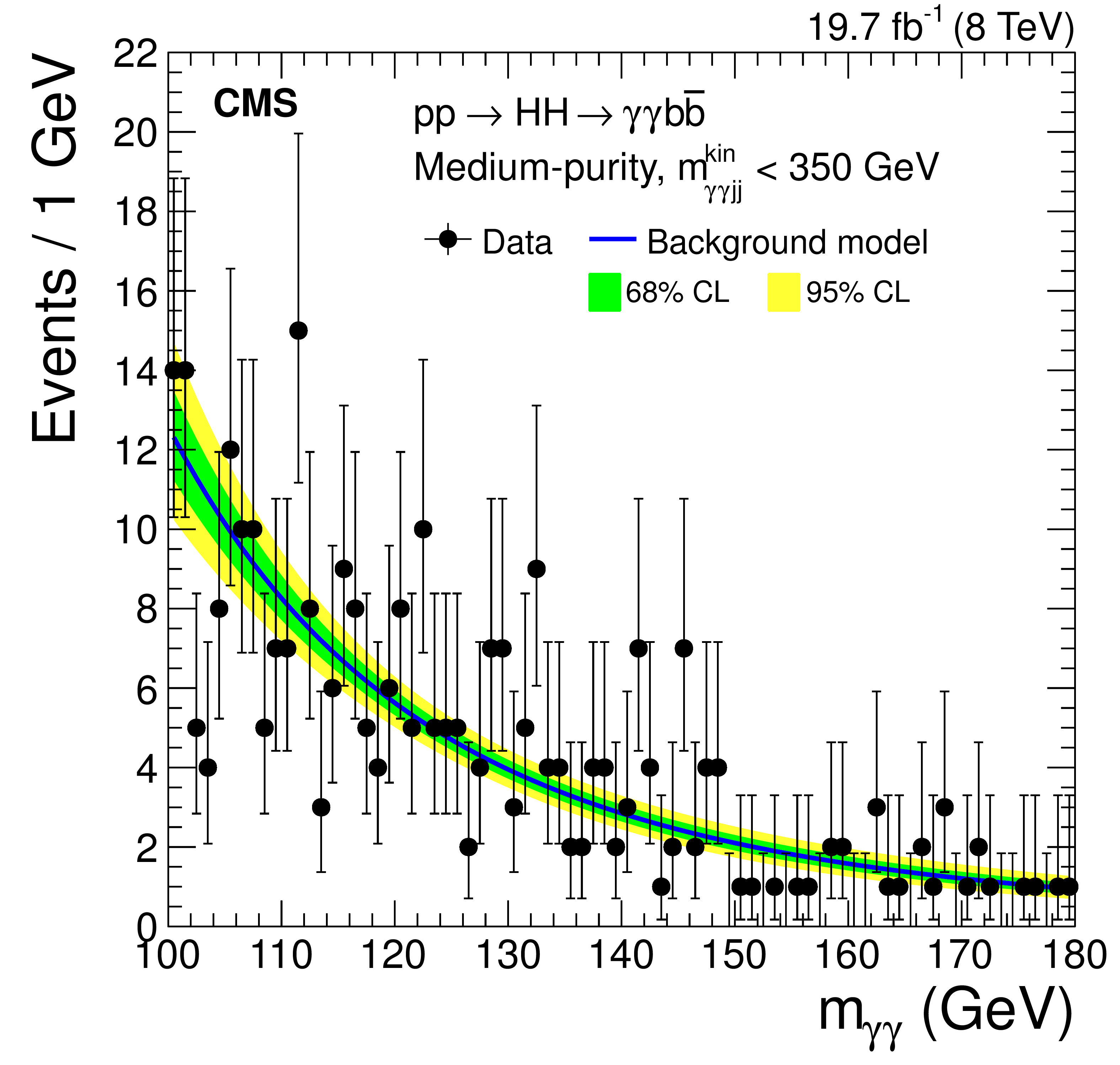
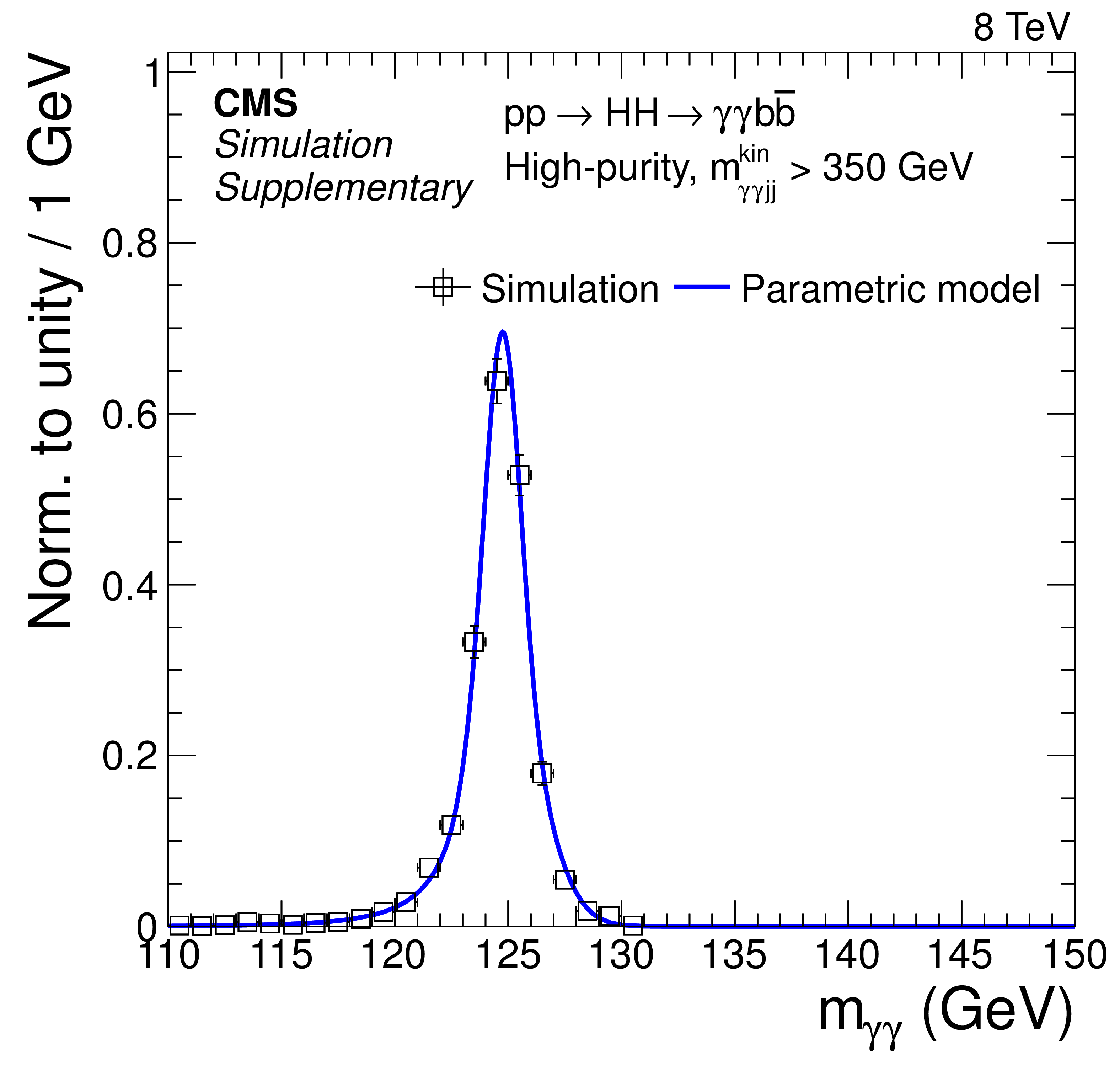
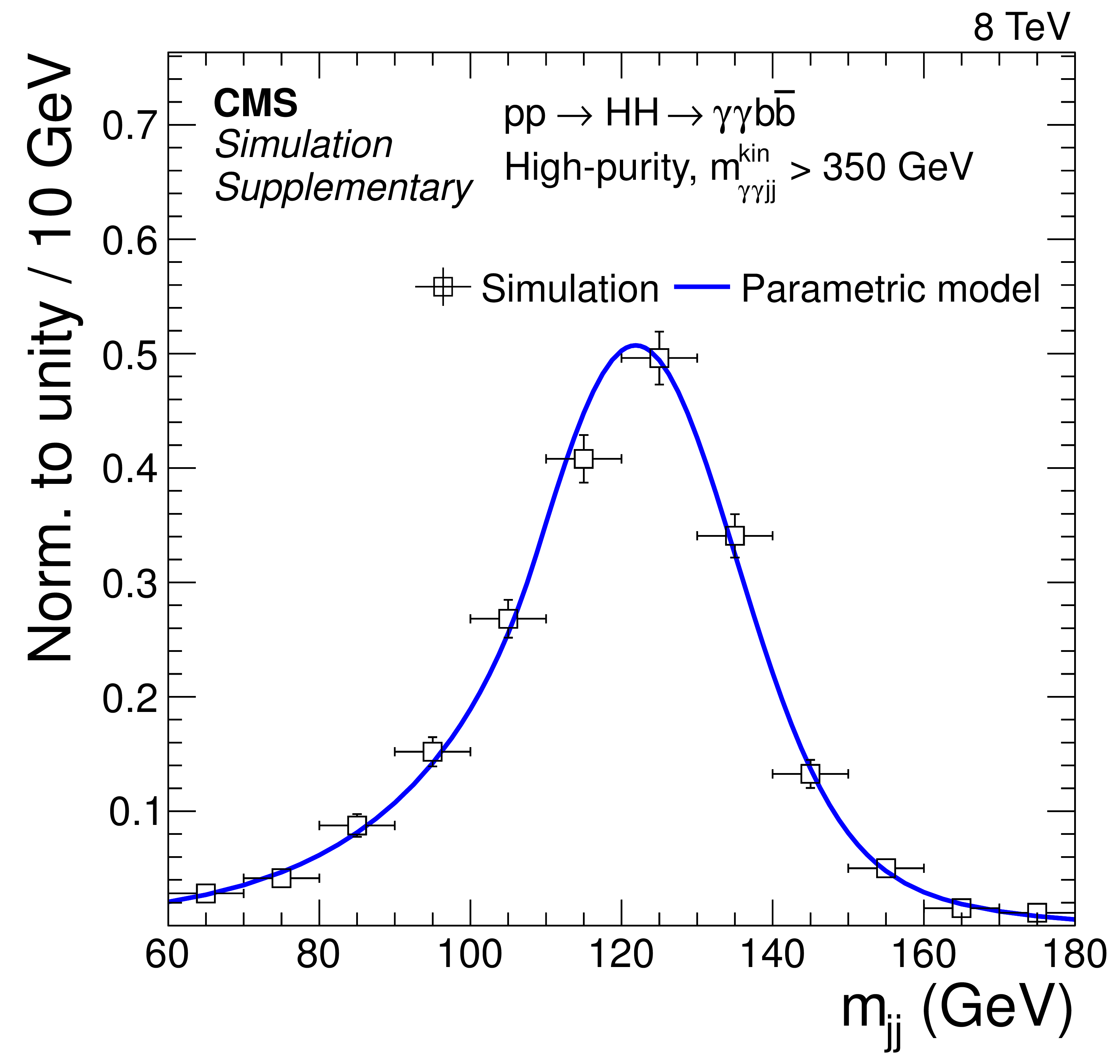
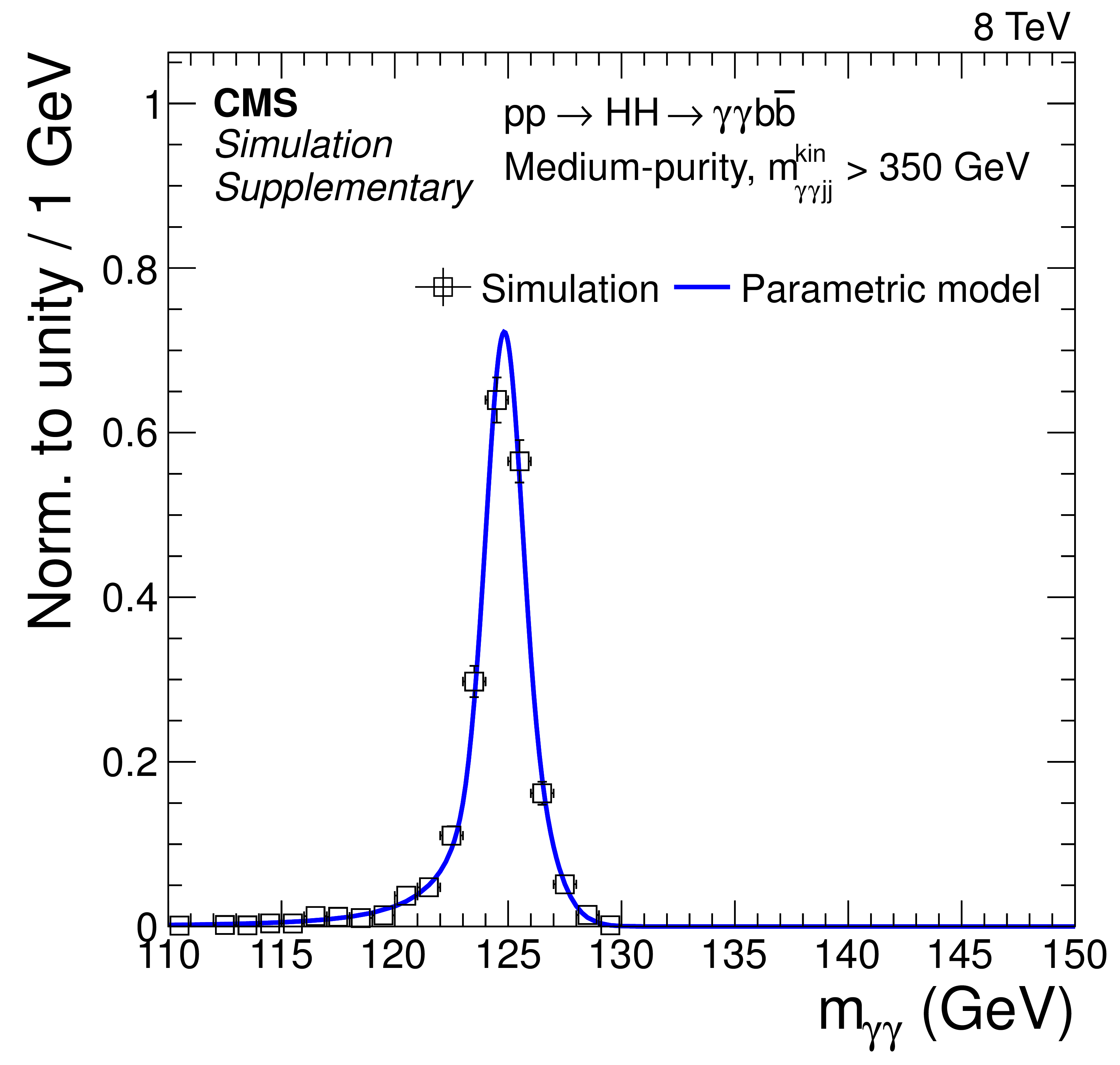
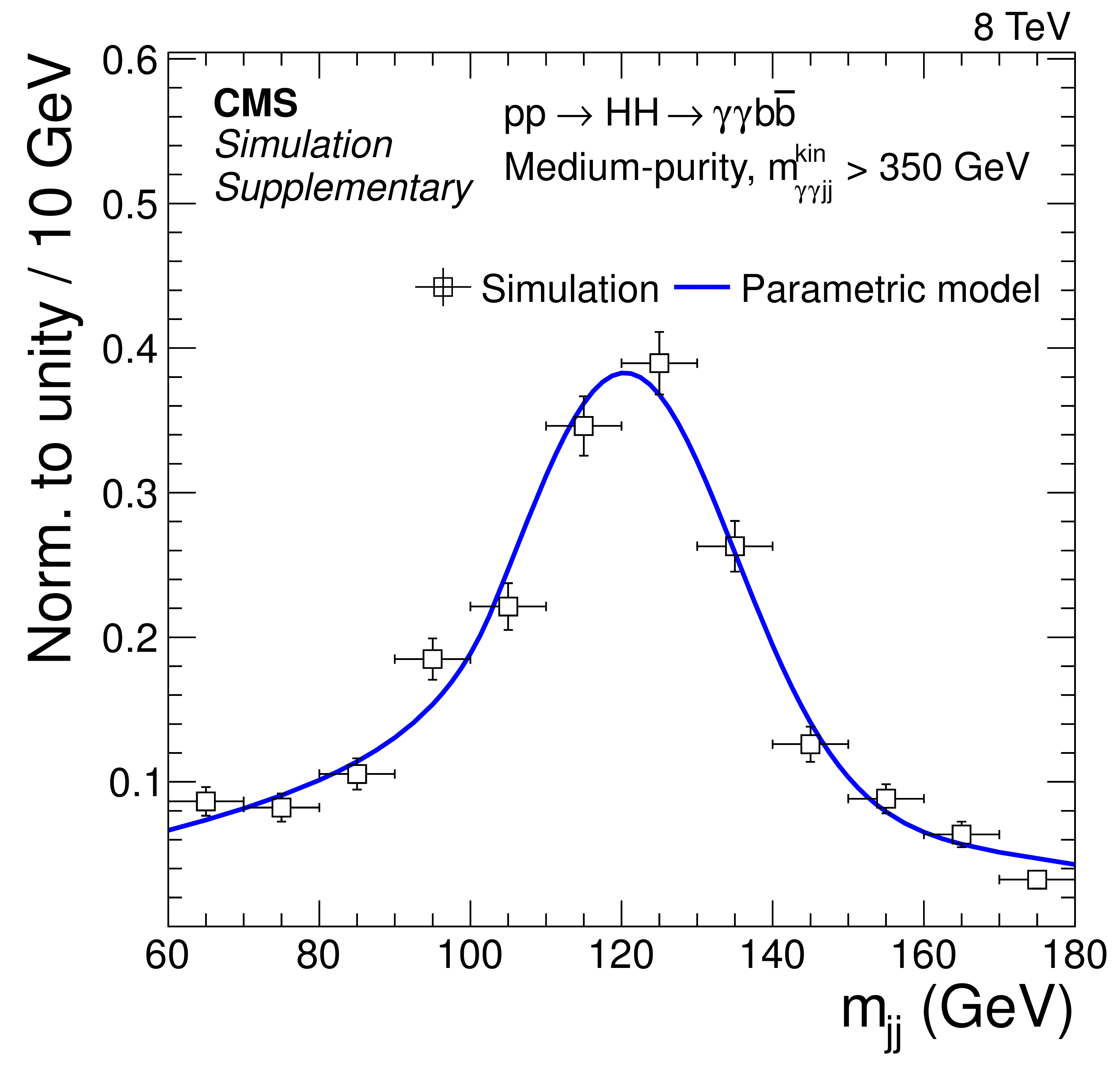
Figure 5-a:
Fits to the nonresonant background contribution in high-$ {m_{\gamma \gamma \mathrm {jj}}^\text {kin}} $ and high-purity category to the $ {m_{\gamma \gamma }} $ (a) and $ {m_\mathrm {jj}} $ spectra (b), and similarly for medium-purity category in (c) and (d), respectively. The fits to the background-only hypothesis are given by the blue curves, along with their 68% and 95% CL contours. |
png pdf |
Figure 5-b:
Fits to the nonresonant background contribution in high-$ {m_{\gamma \gamma \mathrm {jj}}^\text {kin}} $ and high-purity category to the $ {m_{\gamma \gamma }} $ (a) and $ {m_\mathrm {jj}} $ spectra (b), and similarly for medium-purity category in (c) and (d), respectively. The fits to the background-only hypothesis are given by the blue curves, along with their 68% and 95% CL contours. |
png pdf |
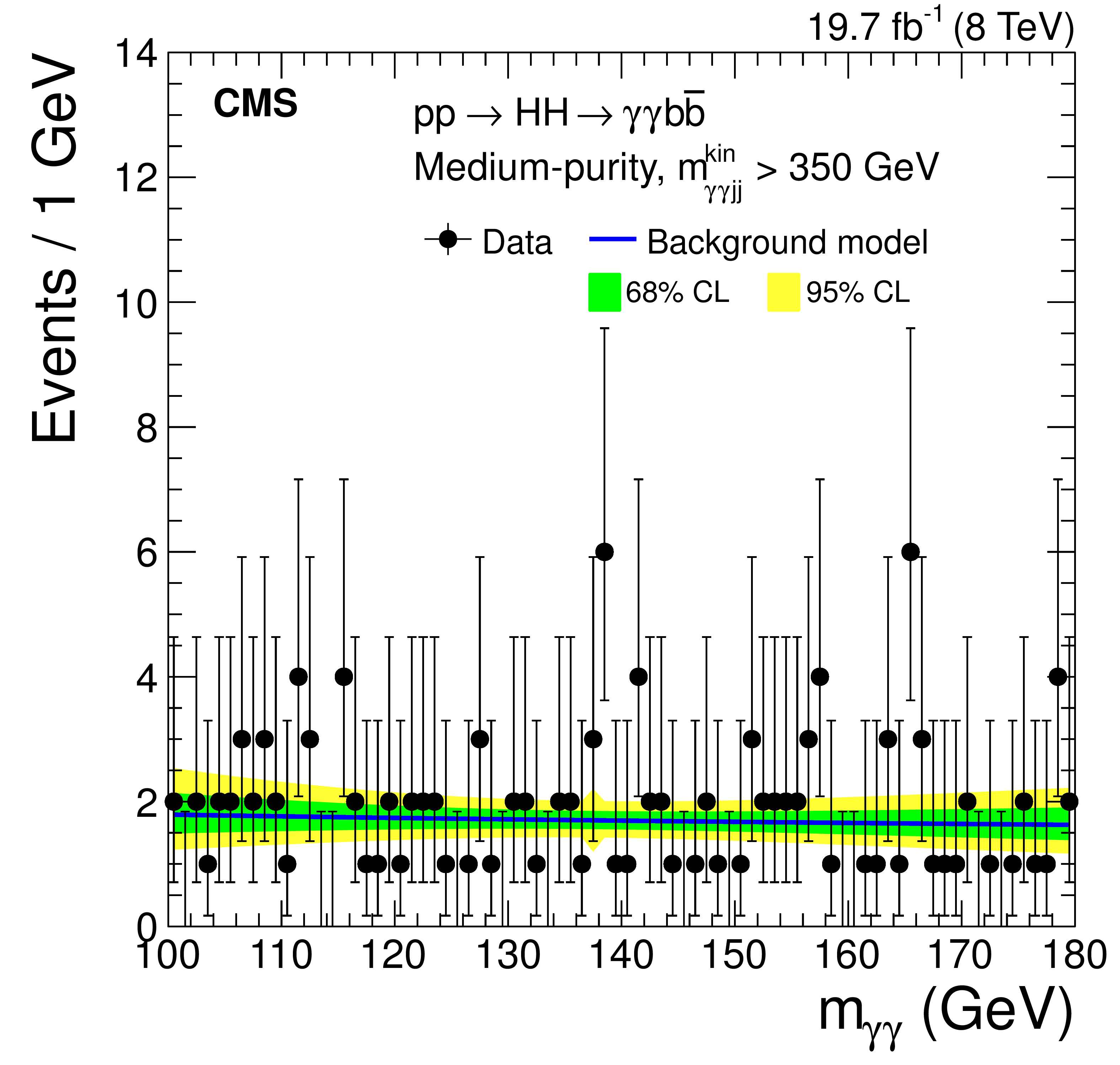
Figure 5-c:
Fits to the nonresonant background contribution in high-$ {m_{\gamma \gamma \mathrm {jj}}^\text {kin}} $ and high-purity category to the $ {m_{\gamma \gamma }} $ (a) and $ {m_\mathrm {jj}} $ spectra (b), and similarly for medium-purity category in (c) and (d), respectively. The fits to the background-only hypothesis are given by the blue curves, along with their 68% and 95% CL contours. |
png pdf |
Figure 5-d:
Fits to the nonresonant background contribution in high-$ {m_{\gamma \gamma \mathrm {jj}}^\text {kin}} $ and high-purity category to the $ {m_{\gamma \gamma }} $ (a) and $ {m_\mathrm {jj}} $ spectra (b), and similarly for medium-purity category in (c) and (d), respectively. The fits to the background-only hypothesis are given by the blue curves, along with their 68% and 95% CL contours. |
png pdf |
Figure 6-a:
Fits to the nonresonant background contribution in low-$ {m_{\gamma \gamma \mathrm {jj}}^\text {kin}} $ and high-purity category to the $ {m_{\gamma \gamma }} $ (a) and $ {m_\mathrm {jj}} $ spectra (b), and similarly for medium-purity category in (c) and (d), respectively. The fits to the background-only hypothesis are given by the blue curves, along with their 68% and 95% CL contours. |
png pdf |
Figure 6-b:
Fits to the nonresonant background contribution in low-$ {m_{\gamma \gamma \mathrm {jj}}^\text {kin}} $ and high-purity category to the $ {m_{\gamma \gamma }} $ (a) and $ {m_\mathrm {jj}} $ spectra (b), and similarly for medium-purity category in (c) and (d), respectively. The fits to the background-only hypothesis are given by the blue curves, along with their 68% and 95% CL contours. |
png pdf |
Figure 6-c:
Fits to the nonresonant background contribution in low-$ {m_{\gamma \gamma \mathrm {jj}}^\text {kin}} $ and high-purity category to the $ {m_{\gamma \gamma }} $ (a) and $ {m_\mathrm {jj}} $ spectra (b), and similarly for medium-purity category in (c) and (d), respectively. The fits to the background-only hypothesis are given by the blue curves, along with their 68% and 95% CL contours. |

png pdf |
Figure 6-d:
Fits to the nonresonant background contribution in low-$ {m_{\gamma \gamma \mathrm {jj}}^\text {kin}} $ and high-purity category to the $ {m_{\gamma \gamma }} $ (a) and $ {m_\mathrm {jj}} $ spectra (b), and similarly for medium-purity category in (c) and (d), respectively. The fits to the background-only hypothesis are given by the blue curves, along with their 68% and 95% CL contours. |
png pdf |
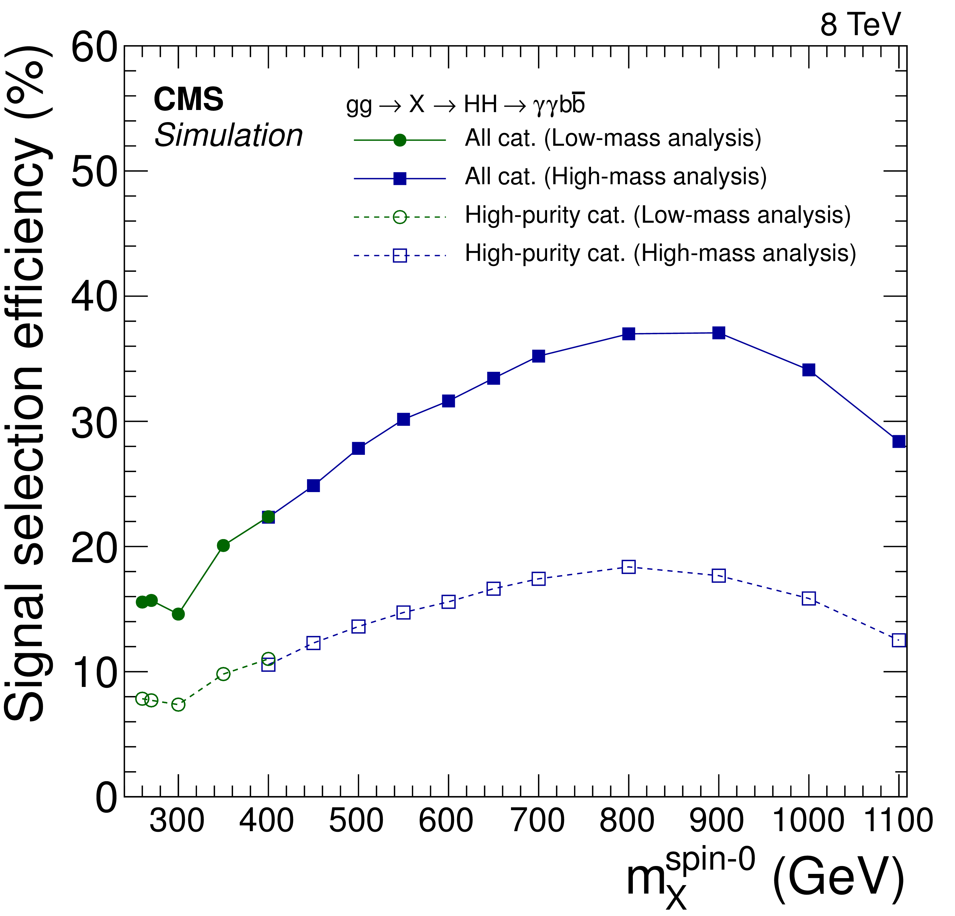
Figure 7:
Resonant signal efficiency for the final selection described in Table 1 and Section 5. The efficiency is shown for a spin-0 hypothesis of a radion particle, but is similar for a spin-2 hypothesis of a KK graviton. The error bars associated with statistical uncertainties are smaller than the size of the markers. |

png pdf |
Figure 8-a:
Signal efficiency for $ {c_2} =$ 0 as function of $ {\kappa _{\lambda }} $ for different values of $ {\kappa _{\mathrm{t}}} $, for the low-$ {m_{\gamma \gamma \mathrm {jj}}^\text {kin}} $ region (a) and high-$ {m_{\gamma \gamma \mathrm {jj}}^\text {kin}} $ region (b). |

png pdf |
Figure 8-b:
Signal efficiency for $ {c_2} =$ 0 as function of $ {\kappa _{\lambda }} $ for different values of $ {\kappa _{\mathrm{t}}} $, for the low-$ {m_{\gamma \gamma \mathrm {jj}}^\text {kin}} $ region (a) and high-$ {m_{\gamma \gamma \mathrm {jj}}^\text {kin}} $ region (b). |
png pdf |
Figure 9-a:
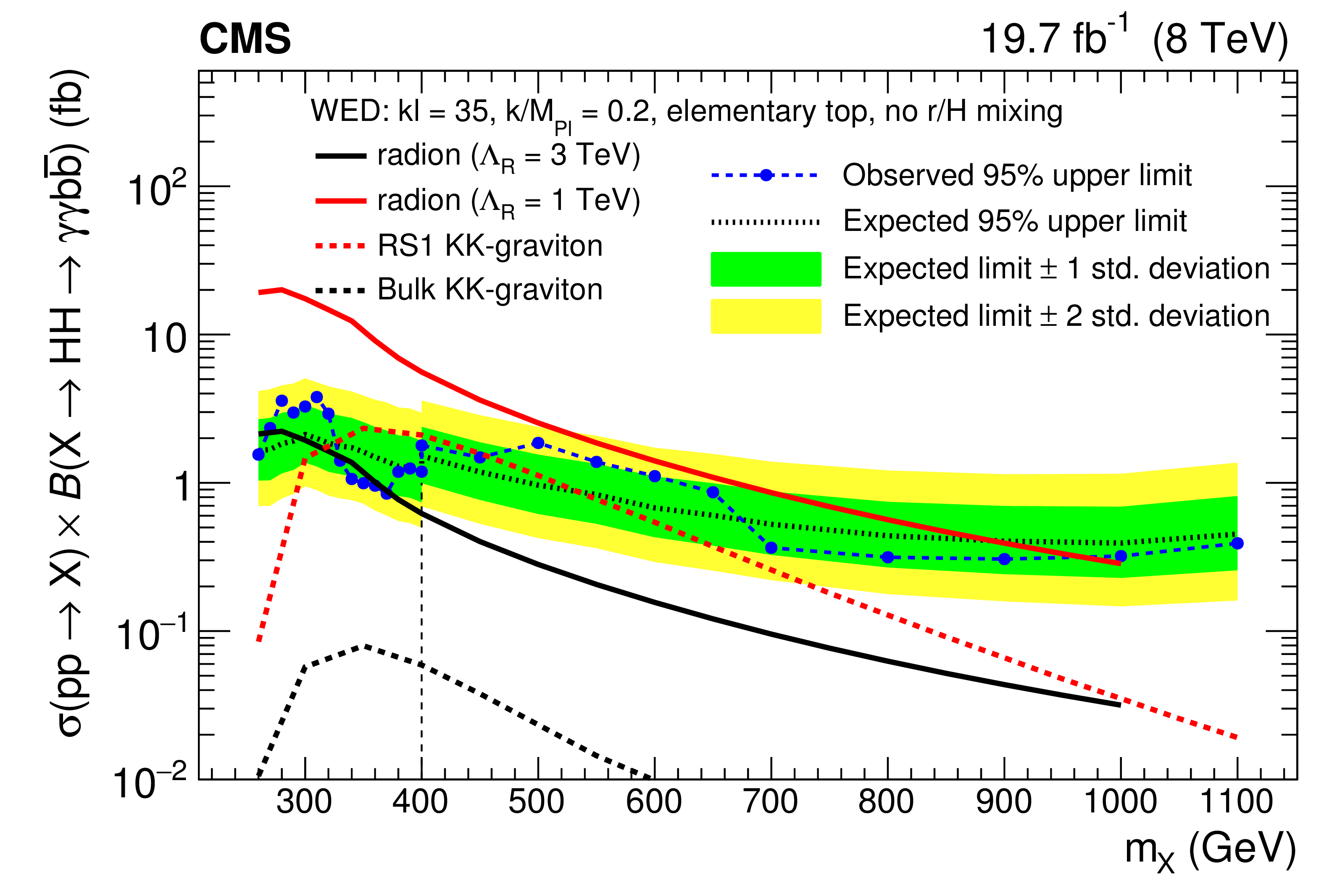
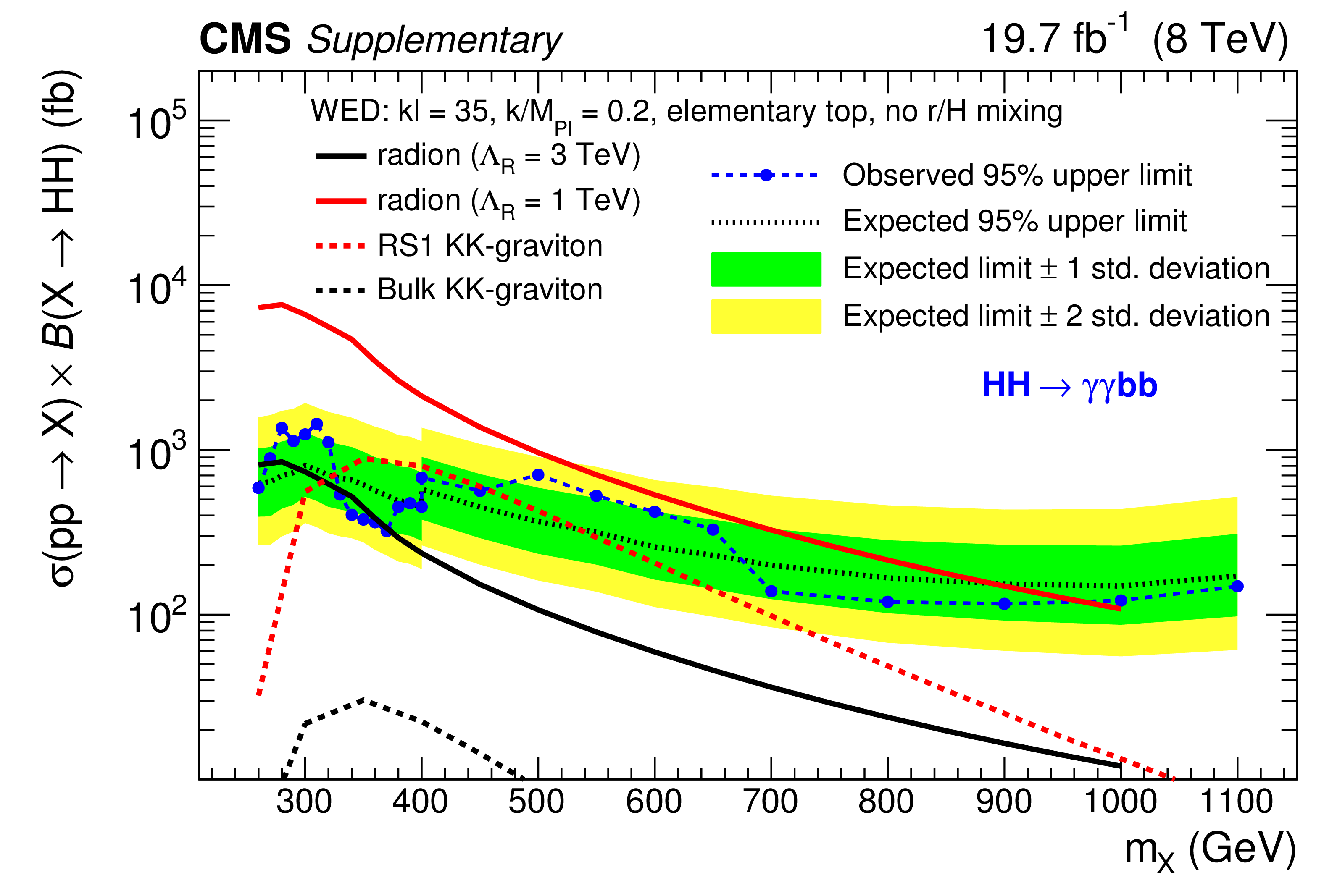
Observed and expected 95% CL upper limits on the product of cross section and the branching fraction $\sigma ( \mathrm{ p p } \to \mathrm {X}) \times \mathcal {B}(\mathrm {X} \to \mathrm{ HH } \to \gamma \gamma \mathrm{ b \bar{b} } )$ obtained through a combination of the two event categories (left ), and in the zoomed view at low-mass (right ). The green and yellow bands represent, respectively, the 1 and 2 standard deviation extensions beyond the expected limit. Also shown are theoretical predictions corresponding to WED models for radions and RS1 KK gravitons. The upper plot with a logarithmic scale for the y-axis also provides the prediction for the production cross section of a bulk KK graviton. The vertical dashed line in the upper plot shows the separation between the low-mass and high-mass analyses. The limits for $ {m_\mathrm {X}} =$ 400 GeV are shown for both methods. |

png pdf |
Figure 9-b:
Observed and expected 95% CL upper limits on the product of cross section and the branching fraction $\sigma ( \mathrm{ p p } \to \mathrm {X}) \times \mathcal {B}(\mathrm {X} \to \mathrm{ HH } \to \gamma \gamma \mathrm{ b \bar{b} } )$ obtained through a combination of the two event categories (left ), and in the zoomed view at low-mass (right ). The green and yellow bands represent, respectively, the 1 and 2 standard deviation extensions beyond the expected limit. Also shown are theoretical predictions corresponding to WED models for radions and RS1 KK gravitons. The upper plot with a logarithmic scale for the y-axis also provides the prediction for the production cross section of a bulk KK graviton. The vertical dashed line in the upper plot shows the separation between the low-mass and high-mass analyses. The limits for $ {m_\mathrm {X}} =$ 400 GeV are shown for both methods. |
png pdf |
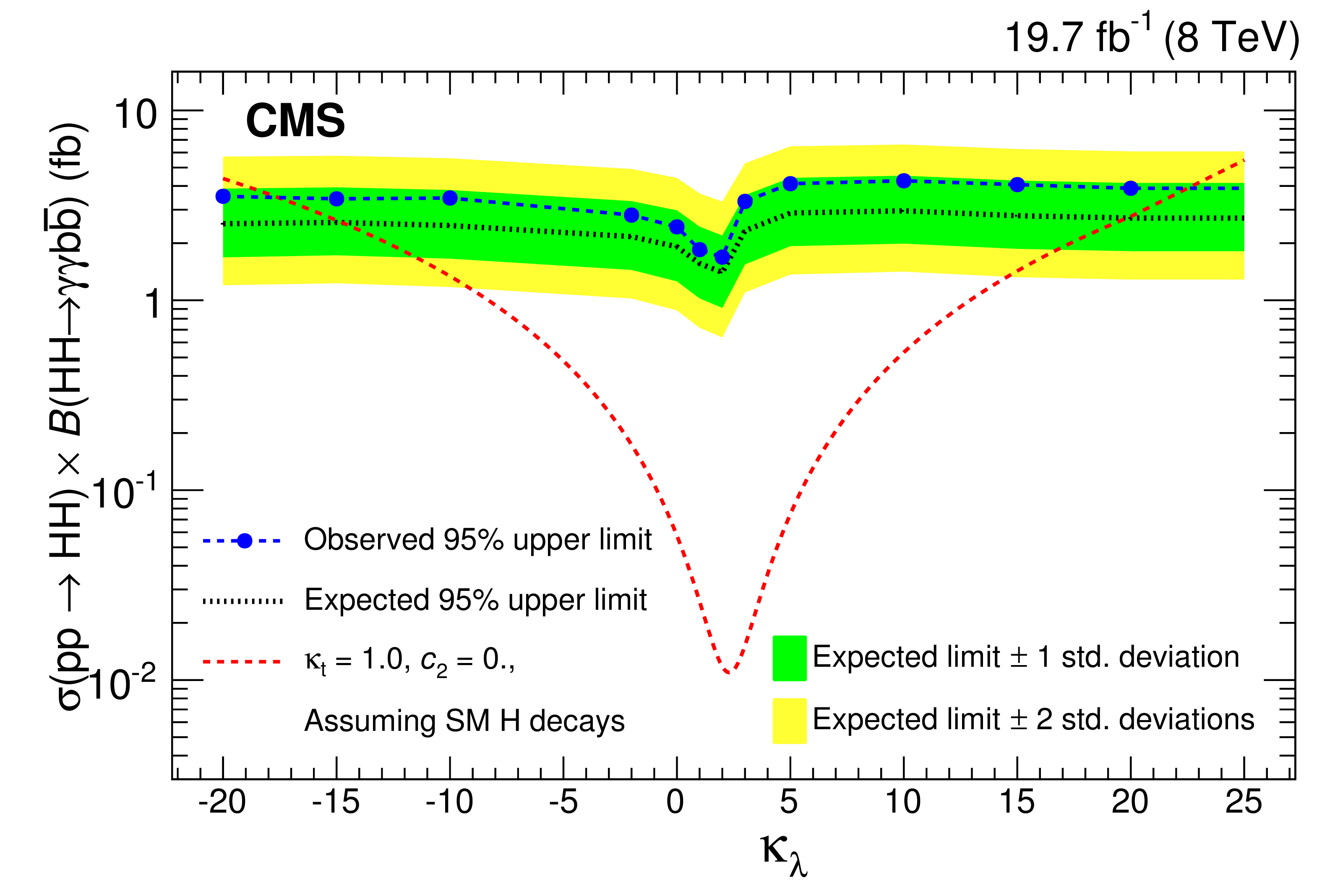
Figure 10:
Observed and expected 95% CL upper limits on the product of cross section and the branching fraction $\sigma (\mathrm{ pp \to HH } ) \times \mathcal {B}( \mathrm{ HH } \to \gamma \gamma \mathrm{ b \bar{b} } )$ for the nonresonant BSM analysis, performed by changing only $ {\kappa _{\lambda }} $, while keeping all other parameters fixed at the SM predictions. |
png pdf |
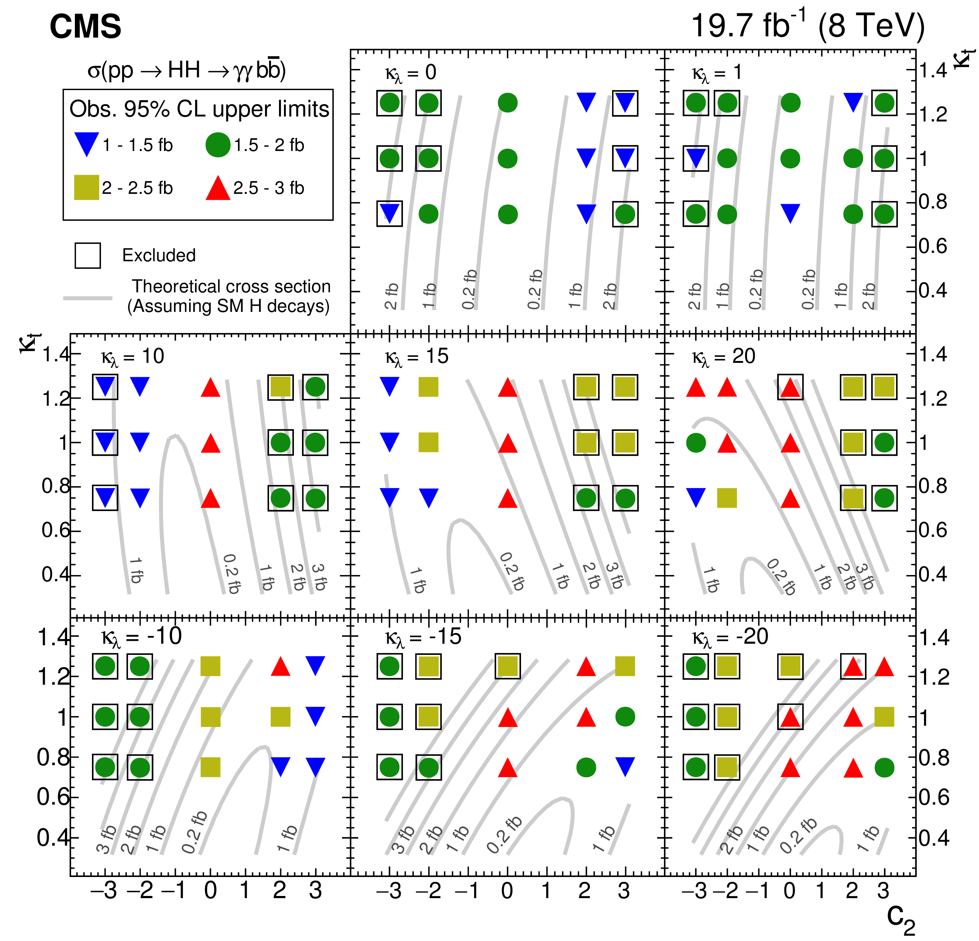
Figure 11:
The observed 95% CL limits for nonresonant two-Higgs production in the $ {c_2} $ and $ {\kappa _{\mathrm{t} }} $ planes for different values of $ {\kappa _{\lambda }} $. The different markers symbolize the range in which the upper limits in the cross sections are relevant. The results are compared to the theoretical prediction. The gray lines represent contours of equal cross section, as calculated using Eq.2. The boxed-in cross section markers provide the combination of parameters excluded at 95% CL . |
| Tables | |
png pdf |
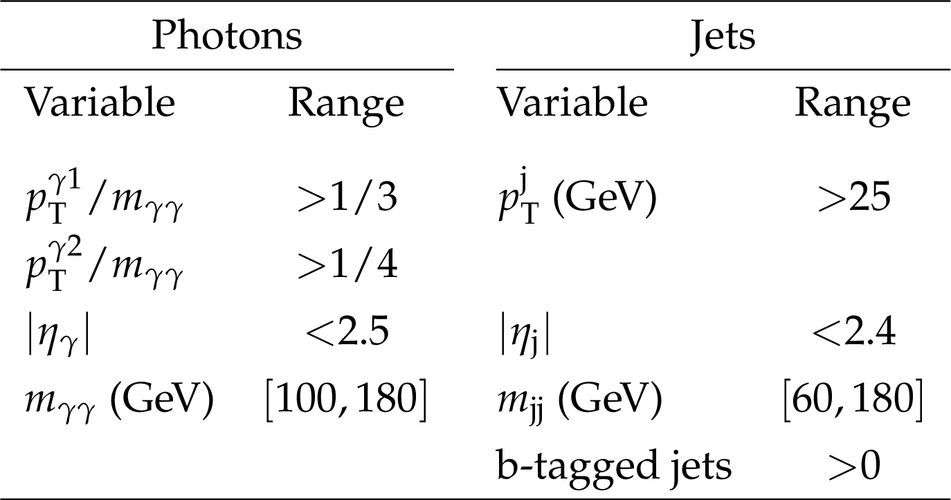
Table 1:
Summary of the analysis preselections. |
png pdf |
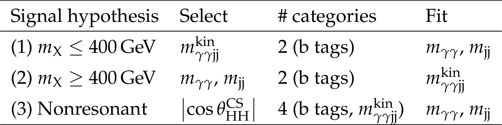
Table 2:
Summary of the search analysis methods. |
png pdf |
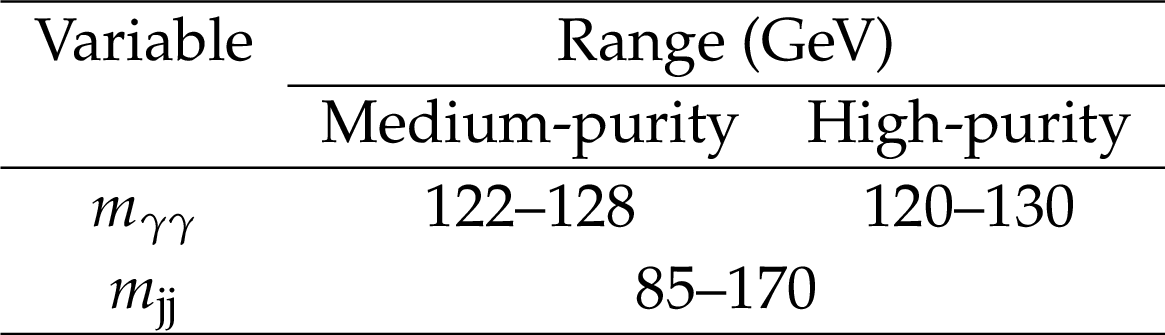
Table 3:
Additional selection criteria applied in the high-mass resonant search. |
png pdf |
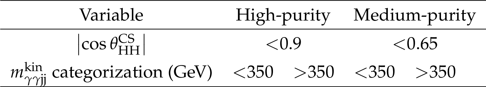
Table 4:
Additional selections applied in the nonresonant searches. |

png pdf |
Table 5:
Summaries of systematic uncertainties. The uncertainty in the b tagging efficiency is anticorrelated between the b tag categories. The uncertainty in the $ {m_{\gamma \gamma \mathrm {jj}}^\text {kin}} $ categorization is anticorrelated between $ {m_{\gamma \gamma \mathrm {jj}}^\text {kin}} $ categories for the nonresonant search. |
png pdf |
Table 6:
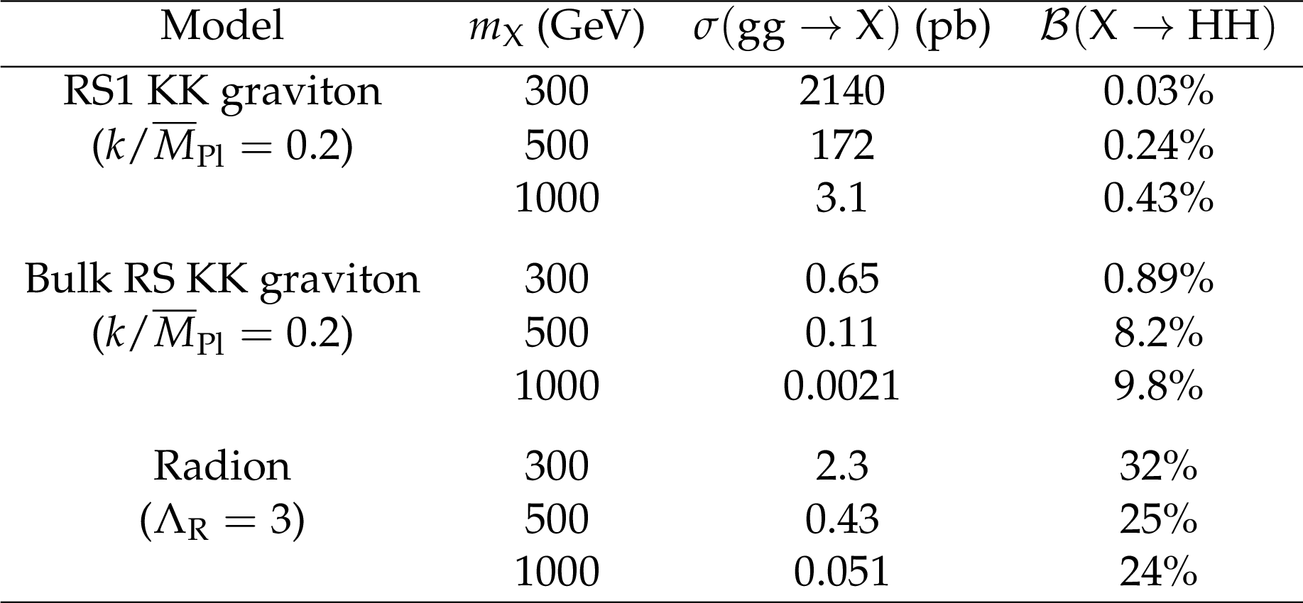
Cross section and branching fractions for the benchmark theories used in this paper\cite {Oliveira:2010uv,Barger:2011qn}. The branching fractions does not depend on $k/ {\overline {M}_\mathrm {Pl}} $, nor on $ {\Lambda _\mathrm {R}} $. |
| Summary |
|
A search is performed by the CMS collaboration for resonant and nonresonant production of two Higgs bosons in the decay channel ${\mathrm{ H }\mathrm{ H }} \to \gamma\gamma \mathrm{ b \bar{b} }$, based on an integrated luminosity of 19.7 fb$^{-1}$ of proton-proton collisions collected at $ \sqrt{s} = $ 8 TeV. The observations are compatible with expectations from standard model processes. No excess is observed over background predictions. Resonances are sought in the mass range between 260 and 1100 GeV. Upper limits at a 95% \CL are extracted on cross sections for the production of new particles decaying to Higgs boson pairs. The limits are compared to BSM predictions, based on the assumption of the existence of a warped extra dimension. A radion with an ultraviolet cutoff ${\Lambda_{\mathrm{R}}} =$ 1 TeV is excluded for masses below 980 GeV. The RS1 KK graviton is excluded with masses between 325 and 450 GeV for $k/{\overline{M}_\mathrm{Pl}} =$ 0.2. For nonresonant production with SM-like kinematics, a 95% \CL upper limit of 1.85 fb is set for the product of the HH cross section and branching fraction, corresponding to a factor 74 larger than the SM value. When only the trilinear Higgs boson coupling is changed, values of the self coupling are excluded for ${\kappa_{\lambda}} < -17$ and ${\kappa_{\lambda}} > 22.5$. The parameter space is also probed for the presence of other anomalous Higgs boson couplings. |
| Additional Figures | |
png pdf |
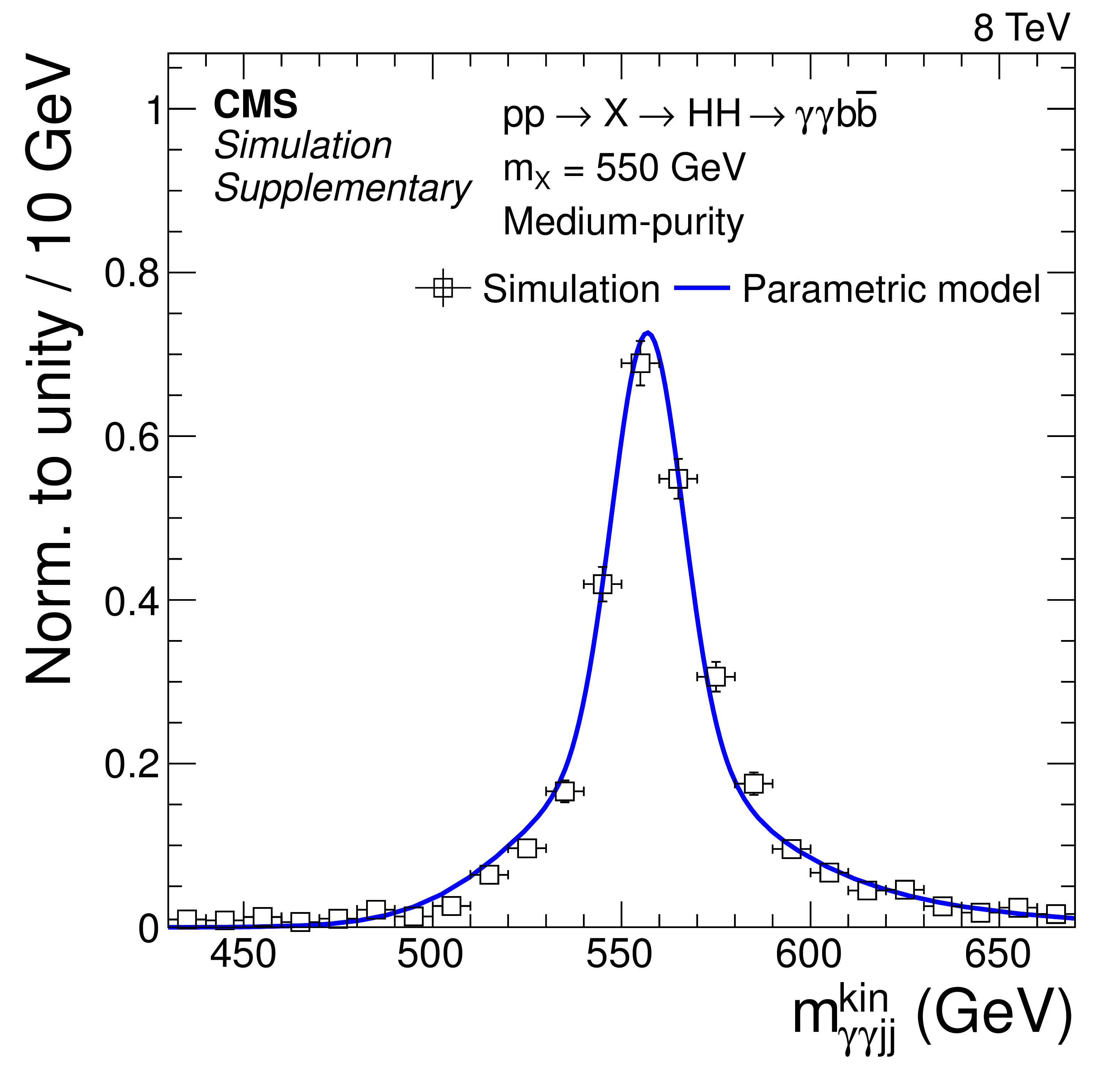
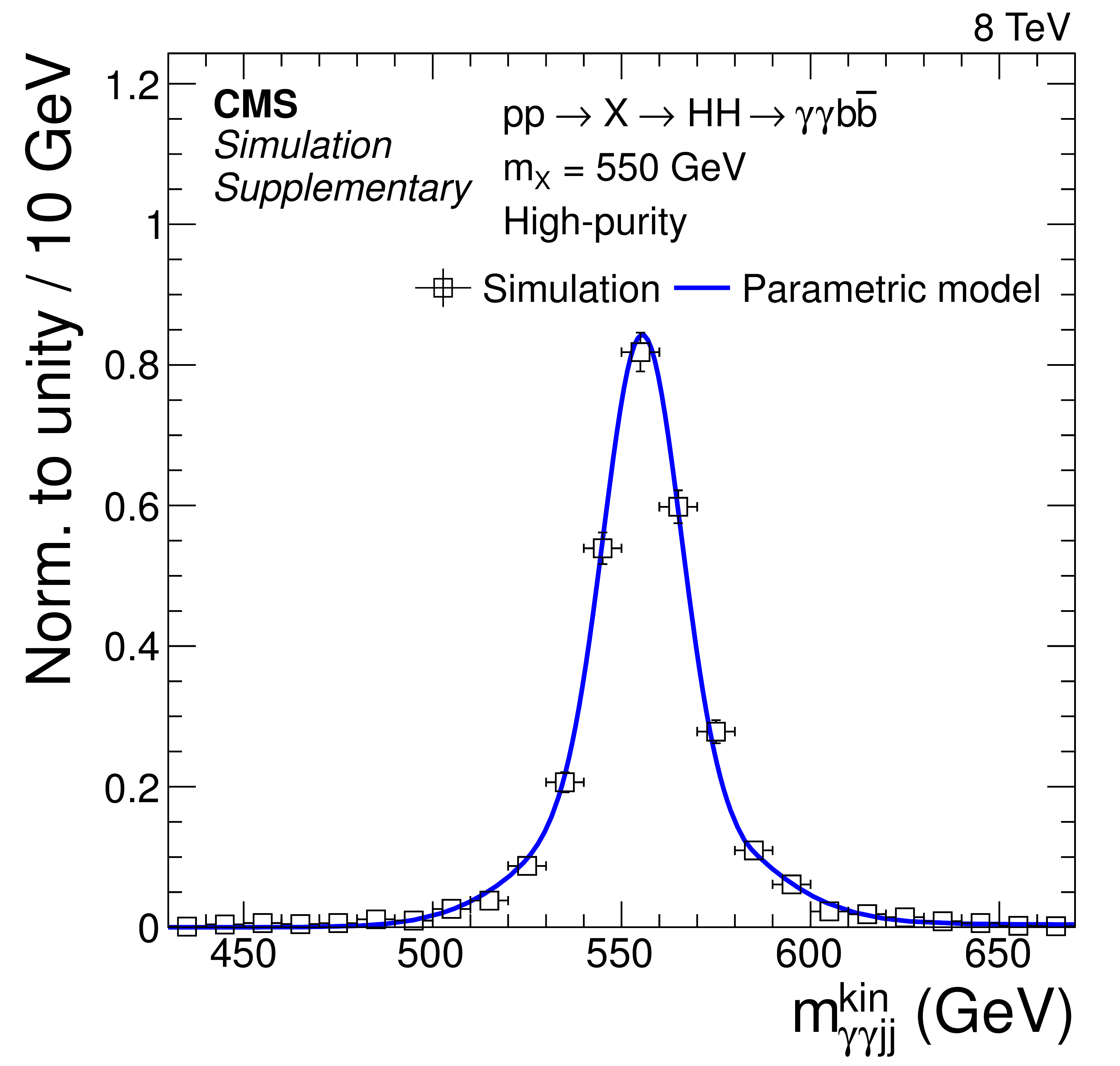
Additional Figure 1-a:
Signal probability densities as function of $ {m_{\gamma \gamma \mathrm {jj}}^\text {kin}} $ for the medium (a) and high-purity (b) categories for a 550 GeV resonance mass hypothesis. |
png pdf |
Additional Figure 1-b:
Signal probability densities as function of $ {m_{\gamma \gamma \mathrm {jj}}^\text {kin}} $ for the medium (a) and high-purity (b) categories for a 550 GeV resonance mass hypothesis. |

png pdf |
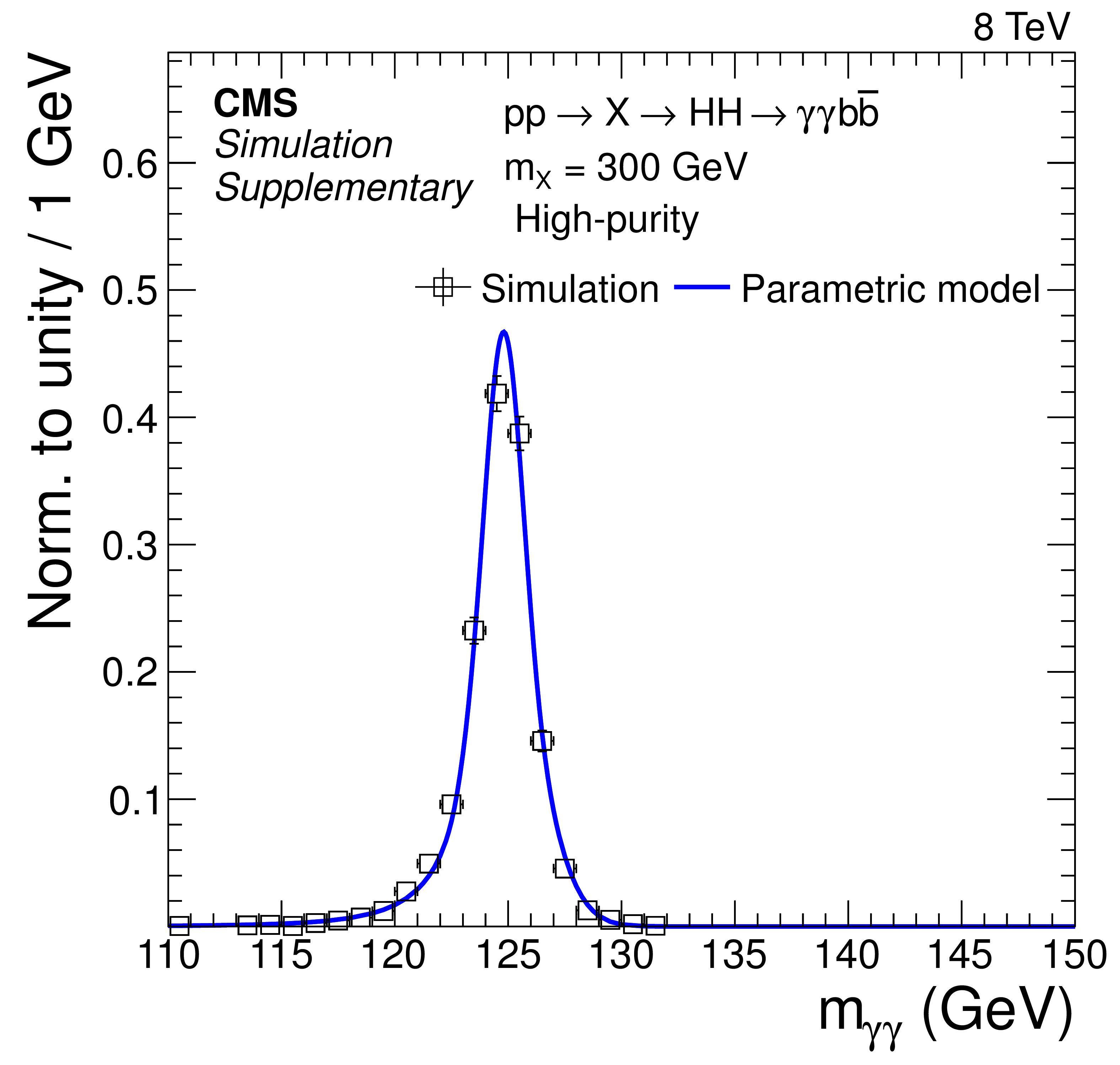
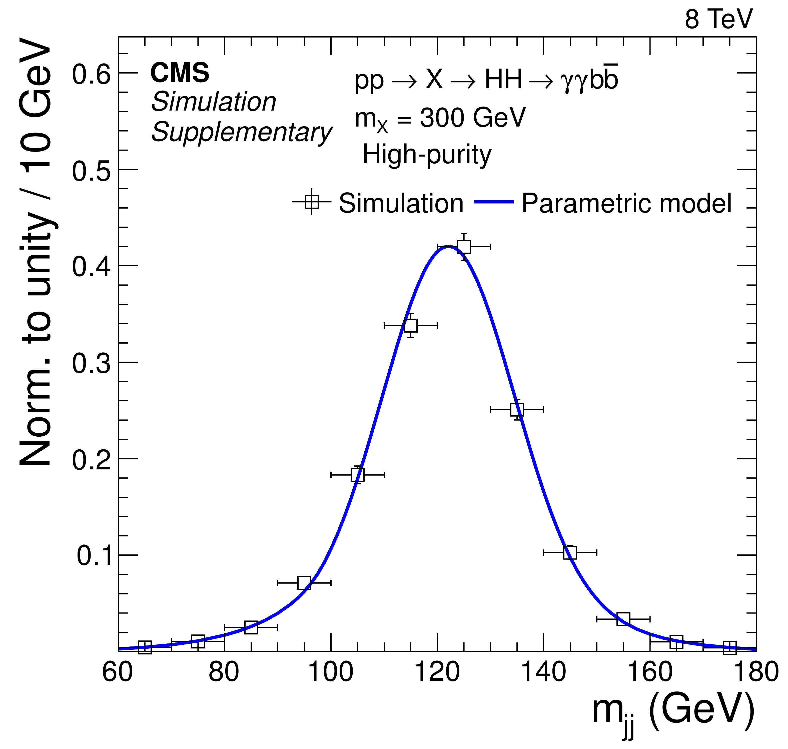
Additional Figure 2-a:
Signal probability densities as function of $ {m_{\gamma \gamma }} $ (a,b) and $ {m_\mathrm {jj}} $ (c,d) for the medium (a,c) and high-purity (b,d) categories for a 300 GeV resonance mass hypothesis. |
png pdf |
Additional Figure 2-b:
Signal probability densities as function of $ {m_{\gamma \gamma }} $ (a,b) and $ {m_\mathrm {jj}} $ (c,d) for the medium (a,c) and high-purity (b,d) categories for a 300 GeV resonance mass hypothesis. |
png pdf |
Additional Figure 2-c:
Signal probability densities as function of $ {m_{\gamma \gamma }} $ (a,b) and $ {m_\mathrm {jj}} $ (c,d) for the medium (a,c) and high-purity (b,d) categories for a 300 GeV resonance mass hypothesis. |
png pdf |
Additional Figure 2-d:
Signal probability densities as function of $ {m_{\gamma \gamma }} $ (a,b) and $ {m_\mathrm {jj}} $ (c,d) for the medium (a,c) and high-purity (b,d) categories for a 300 GeV resonance mass hypothesis. |
png pdf |
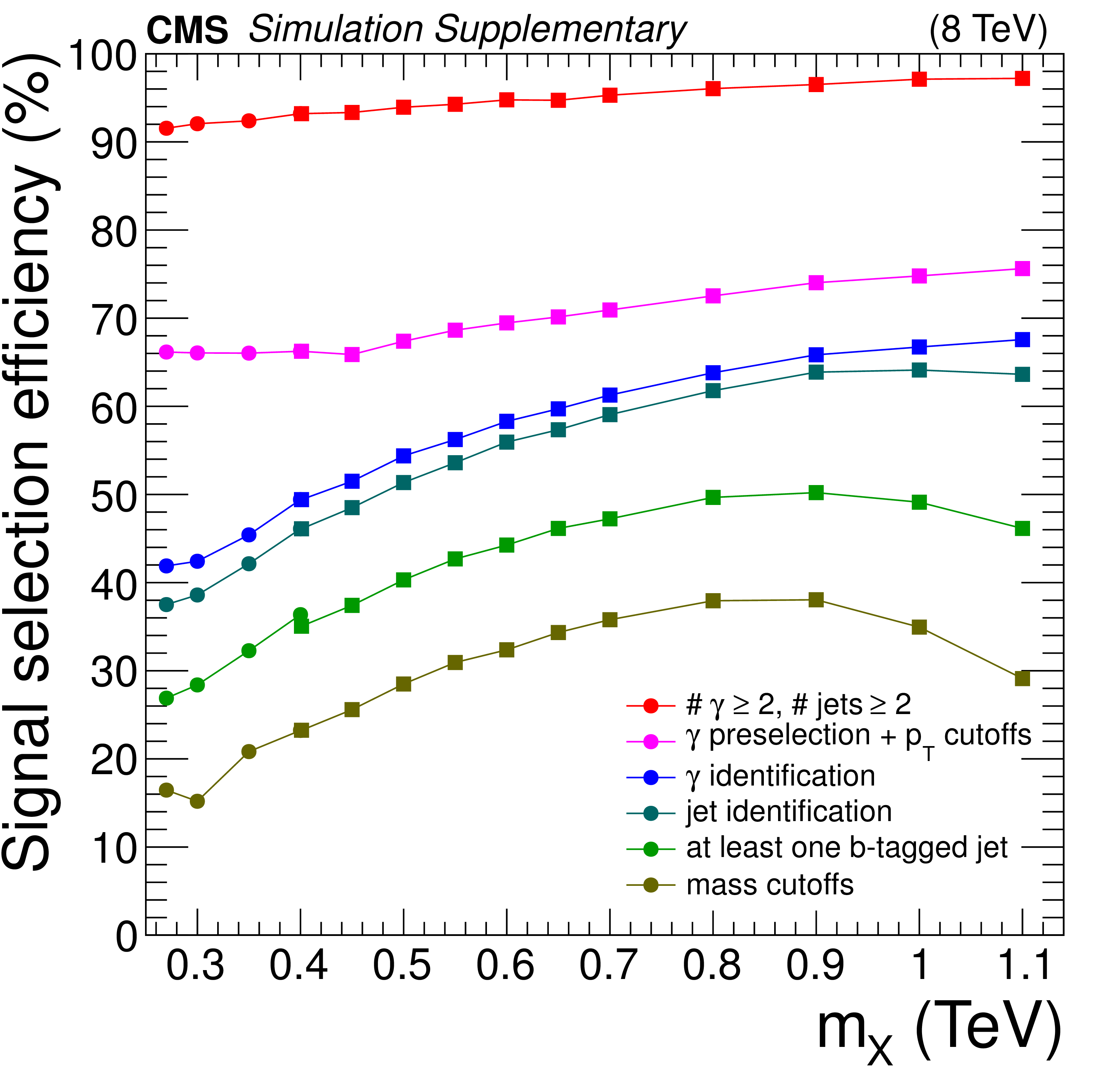
Additional Figure 3:
Efficiency associated with the consecutive selections described in Section 4. Red: at least 2 photons required in the event, with the usual photon supercluster acceptance requirements, $ {p_\mathrm {T}^{\gamma 1}} >$ 40 GeV, $ {p_\mathrm {T}^{\gamma 2}} >$ 30 GeV, at least 2 jets in the event with following $ {p_\mathrm {T}^\mathrm {j}} >$ 10 GeV, $ {\Delta R_{\gamma \mathrm {j}}} >$ 0.3, $| {\eta _\mathrm {j}} | <$ 2.5. Pink: preselection cutoffs required on the photons $ {p_\mathrm {T}^{\gamma 1}} / {m_{\gamma \gamma }} >$ 1/3 and $ {p_\mathrm {T}^{\gamma 2}} / {m_{\gamma \gamma }} >$ 1/4, as well as an $ {m_{\gamma \gamma }} $ mass window 100-180 GeV. Blue: cutoff-based photon identification is required on the two photons. Cyan: the jets are required to pass the jet identification criteria, $ {p_\mathrm {T}^\mathrm {j}} >$ 25 GeV, $ {\Delta R_{\gamma \mathrm {j}}} >$ 0.5. Green: at least one jet is required to be b tagged by the CSV algorithm. Dark yellow: the analysis cutoff applied for $ {m_{\gamma \gamma \mathrm {jj}}^\text {kin}} $ for the low-mass analysis (circles) ; $ {m_\mathrm {jj}} $ and $ {m_{\gamma \gamma }} $ cutoffs for the high-mass analysis (squares). Note that the final efficiency (after the mass selection) in this plot does not contain the data/MC correction factors (in particular the b tag ones) and therefore a minor disagreement with the final efficiency plot in Fig.7 can be expected. |
png pdf |
Additional Figure 4:
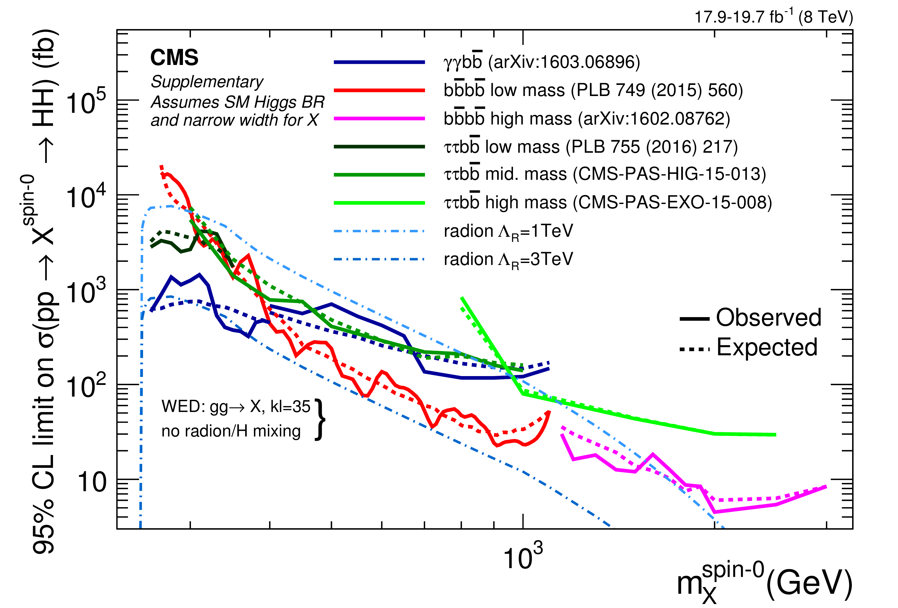
Observed and expected 95% CL upper limits on the product of cross section and the branching fraction $\sigma (gg \to X) \times B(X \to {\mathrm{ H } \mathrm{ H } } )$ obtained by a combination of two categories. The green and yellow bands represent, respectively, the 1 and 2 standard deviations around the expected limit. Theory lines corresponding to WED models with radion, RS1 KK-graviton and bulk KK-graviton are also shown. |
png pdf |
Additional Figure 5:
Observed and expected 95% CL upper limits on the product of cross section and the branching fraction $\sigma (gg \to X) \times B(X \to {\mathrm{ H } \mathrm{ H } } )$ obtained by different analyses assuming spin-0 hypothesis. Theory lines corresponding to WED models with radion are also shown. |
png pdf |
Additional Figure 6-a:
Signal probability densities for SM $ {\mathrm{ H } \mathrm{ H } } $ production: $ {m_{\gamma \gamma }} $ (a,c) and $ {m_\mathrm {jj}} $ (b,d) for small $ {m_{\gamma \gamma \mathrm {jj}}^\text {kin}} $ values. The categories are high-purity (a,b); medium-purity (c,d). |

png pdf |
Additional Figure 6-b:
Signal probability densities for SM $ {\mathrm{ H } \mathrm{ H } } $ production: $ {m_{\gamma \gamma }} $ (a,c) and $ {m_\mathrm {jj}} $ (b,d) for small $ {m_{\gamma \gamma \mathrm {jj}}^\text {kin}} $ values. The categories are high-purity (a,b); medium-purity (c,d). |
png pdf |
Additional Figure 6-c:
Signal probability densities for SM $ {\mathrm{ H } \mathrm{ H } } $ production: $ {m_{\gamma \gamma }} $ (a,c) and $ {m_\mathrm {jj}} $ (b,d) for small $ {m_{\gamma \gamma \mathrm {jj}}^\text {kin}} $ values. The categories are high-purity (a,b); medium-purity (c,d). |
png pdf |
Additional Figure 6-d:
Signal probability densities for SM $ {\mathrm{ H } \mathrm{ H } } $ production: $ {m_{\gamma \gamma }} $ (a,c) and $ {m_\mathrm {jj}} $ (b,d) for small $ {m_{\gamma \gamma \mathrm {jj}}^\text {kin}} $ values. The categories are high-purity (a,b); medium-purity (c,d). |
png pdf |
Additional Figure 7-a:
Signal probability densities for SM $ {\mathrm{ H } \mathrm{ H } } $ production: $ {m_{\gamma \gamma }} $ (a,c) and $ {m_\mathrm {jj}} $ (b,d) for high $ {m_{\gamma \gamma \mathrm {jj}}^\text {kin}} $ values. The categories are high-purity (a,b); medium-purity (c,d). |
png pdf |
Additional Figure 7-b:
Signal probability densities for SM $ {\mathrm{ H } \mathrm{ H } } $ production: $ {m_{\gamma \gamma }} $ (a,c) and $ {m_\mathrm {jj}} $ (b,d) for high $ {m_{\gamma \gamma \mathrm {jj}}^\text {kin}} $ values. The categories are high-purity (a,b); medium-purity (c,d). |
png pdf |
Additional Figure 7-c:
Signal probability densities for SM $ {\mathrm{ H } \mathrm{ H } } $ production: $ {m_{\gamma \gamma }} $ (a,c) and $ {m_\mathrm {jj}} $ (b,d) for high $ {m_{\gamma \gamma \mathrm {jj}}^\text {kin}} $ values. The categories are high-purity (a,b); medium-purity (c,d). |
png pdf |
Additional Figure 7-d:
Signal probability densities for SM $ {\mathrm{ H } \mathrm{ H } } $ production: $ {m_{\gamma \gamma }} $ (a,c) and $ {m_\mathrm {jj}} $ (b,d) for high $ {m_{\gamma \gamma \mathrm {jj}}^\text {kin}} $ values. The categories are high-purity (a,b); medium-purity (c,d). |
png pdf |
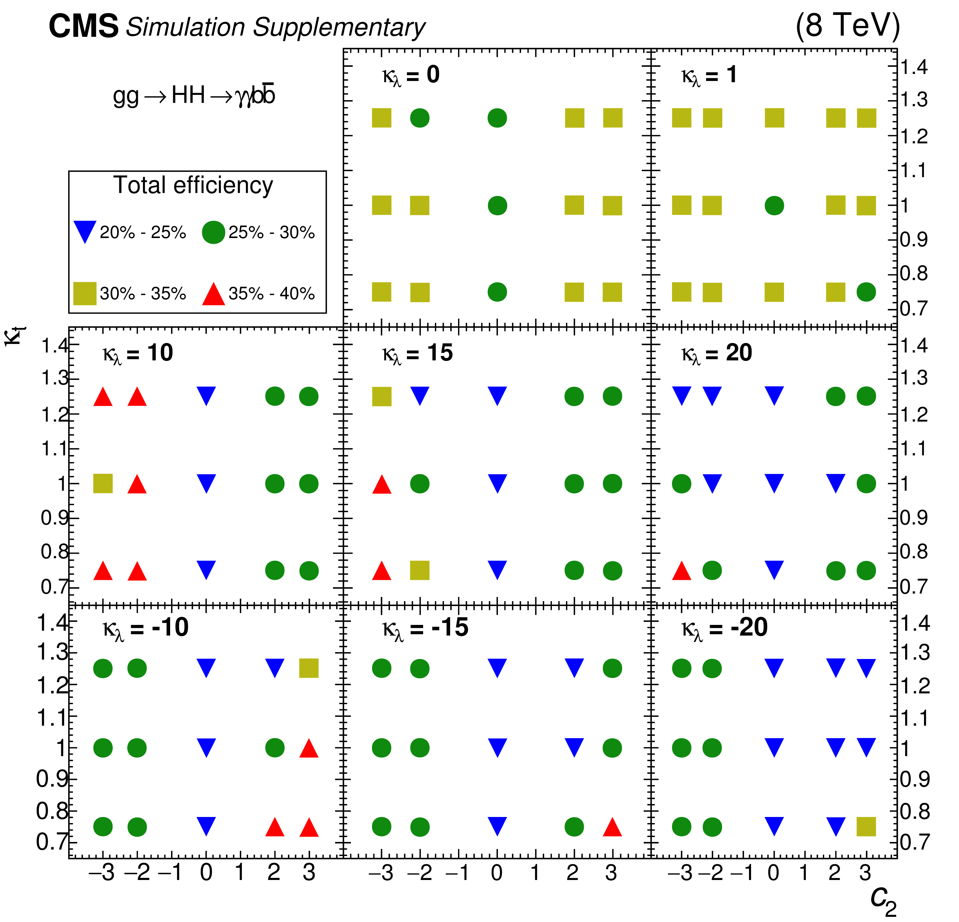
Additional Figure 8:
Selection efficiency of the nonresonant two-Higgs boson production samples summed over four categories: in the $ {c_2} $ and $ {\kappa _{\mathrm{ t } }} $ planes for different values of $ {\kappa _{\lambda }} $. |
png pdf |
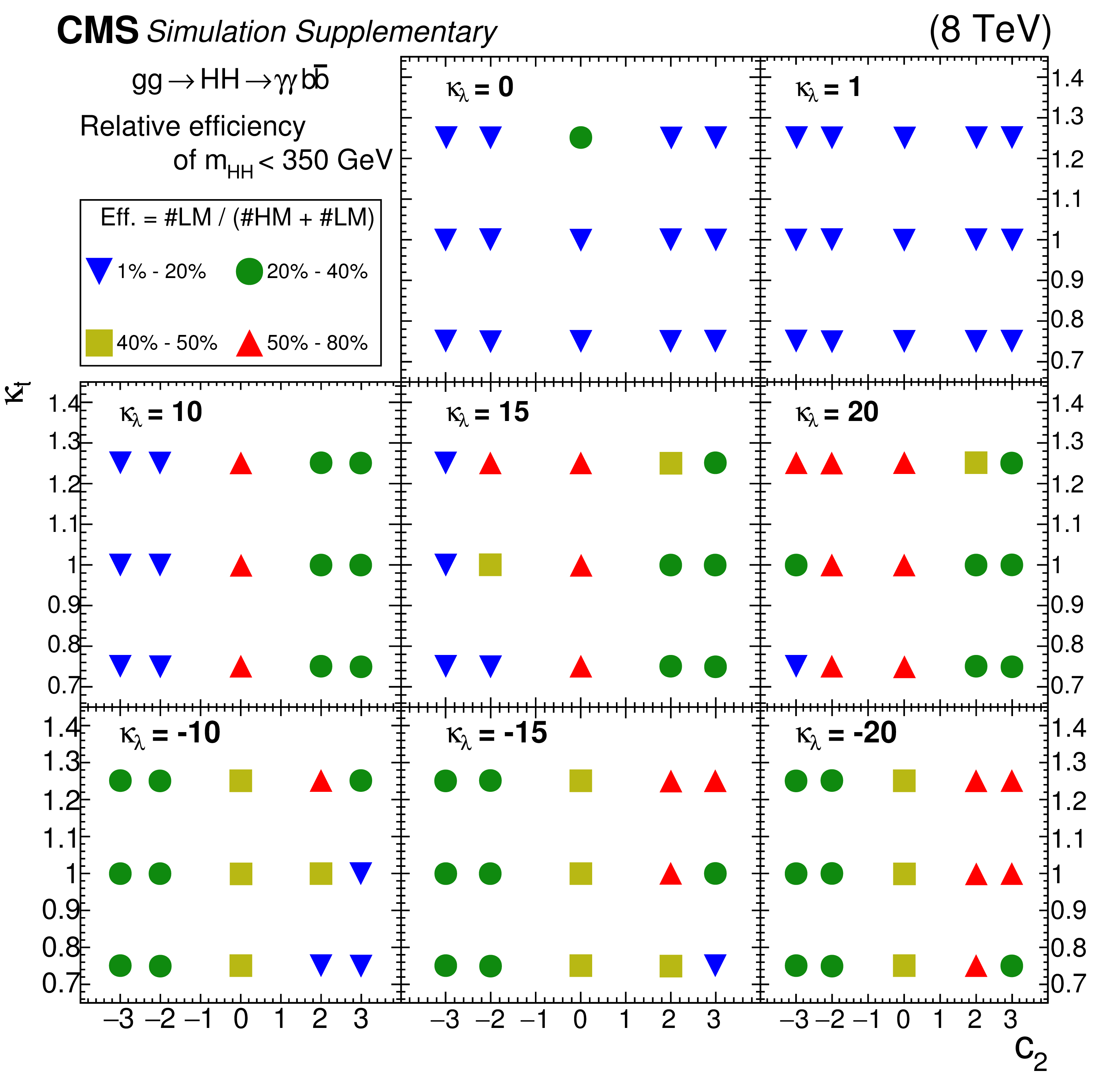
Additional Figure 9:
The fraction of signal events in the $ {m_{\gamma \gamma \mathrm {jj}}^\text {kin}} <$ 350 GeV category (LM), obtained summing over b-tagging categories, with respect to the total number of signal events in $ {m_{\gamma \gamma \mathrm {jj}}^\text {kin}} < $ 350 GeV and $ {m_{\gamma \gamma \mathrm {jj}}^\text {kin}} > $ 350 GeV categories (HM). The fraction is shown in the $ {c_2} $ and $ {\kappa _{\mathrm{ t } }} $ planes for different values of $ {\kappa _{\lambda }} $. |

png pdf |
Additional Figure 10:
Comparison of simulated $ {m_{\gamma \gamma \mathrm {jj}}^\text {kin}} $ and $ {m_{\gamma \gamma \mathrm {jj}}} $ spectra for the spin-0 radion signal at $ {m_\mathrm {X}} =$ 300 and 700 GeV, and $\gamma \gamma /\gamma {\rm jet} + \geq $ 2-jets background, after object selections on photons and jets and a requirement of at least one b-tagged jet. All spectra are normalized to unity. |
png pdf |
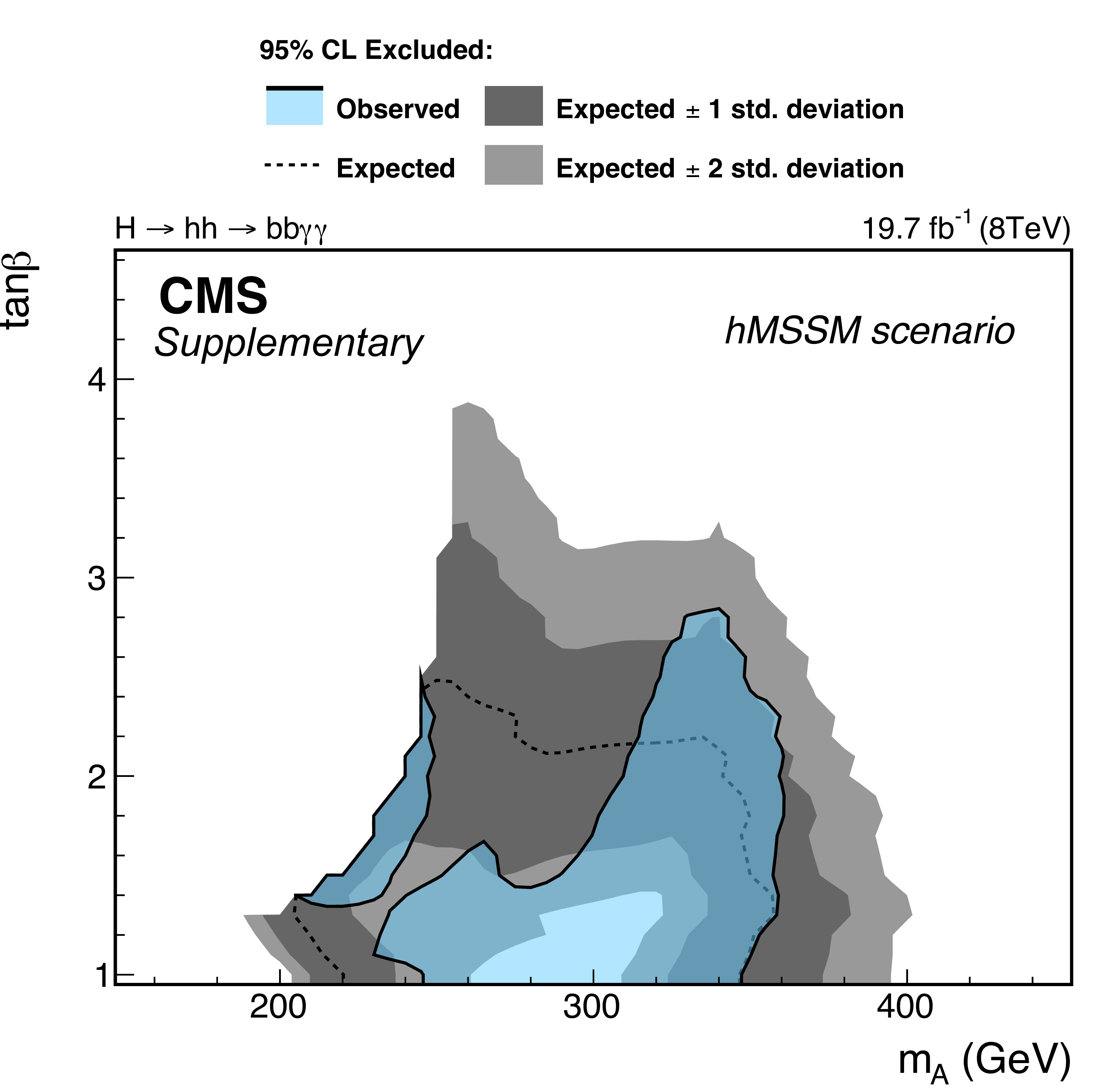
Additional Figure 11:
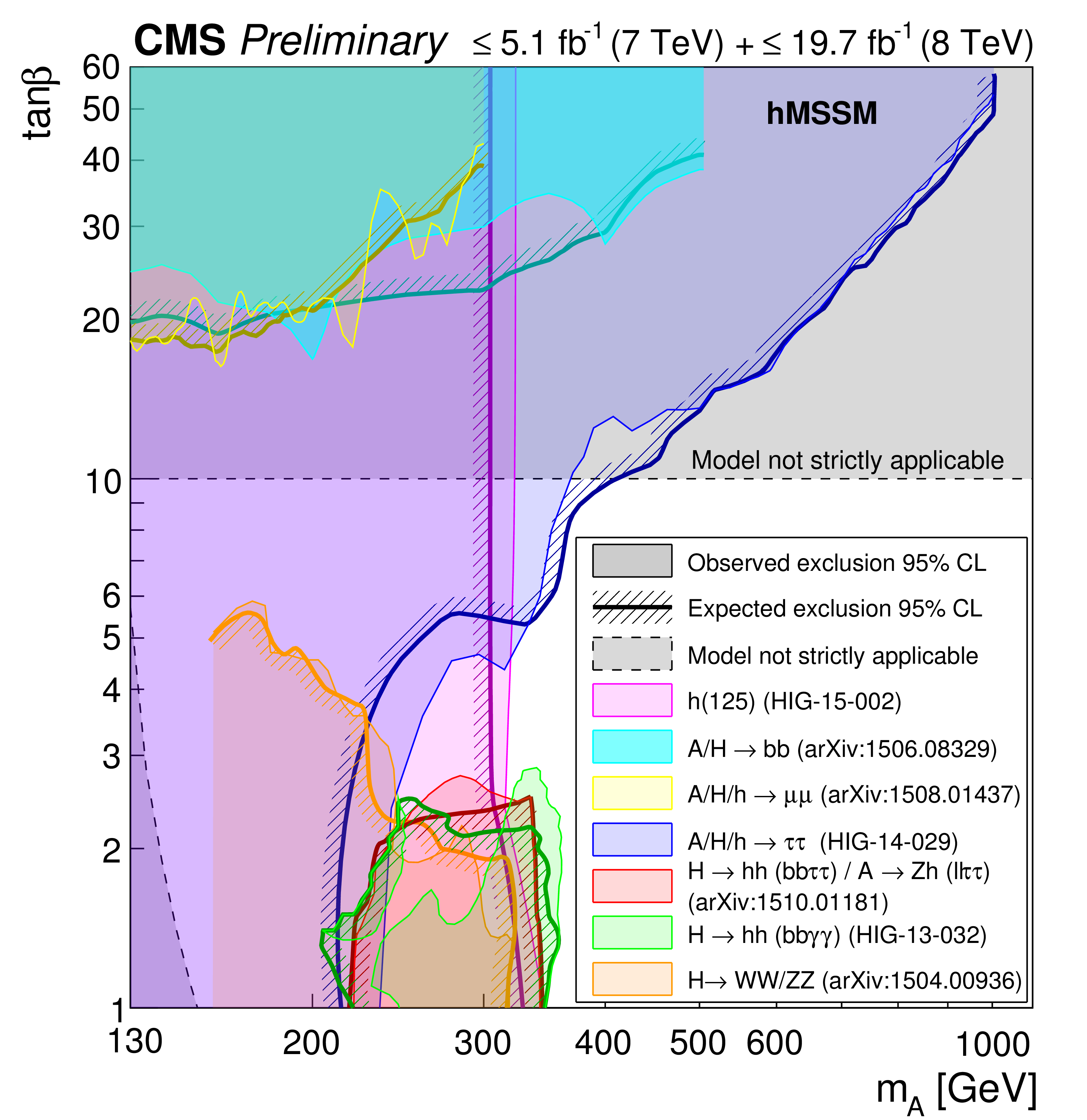
Observed and expected median 95% CL limit interpreted within the framework of hMSSM. This Additional Figure is a zoomed copy of this plot in CMS-PAS-HIG-16-007. |
| Additional Tables | |
png pdf |
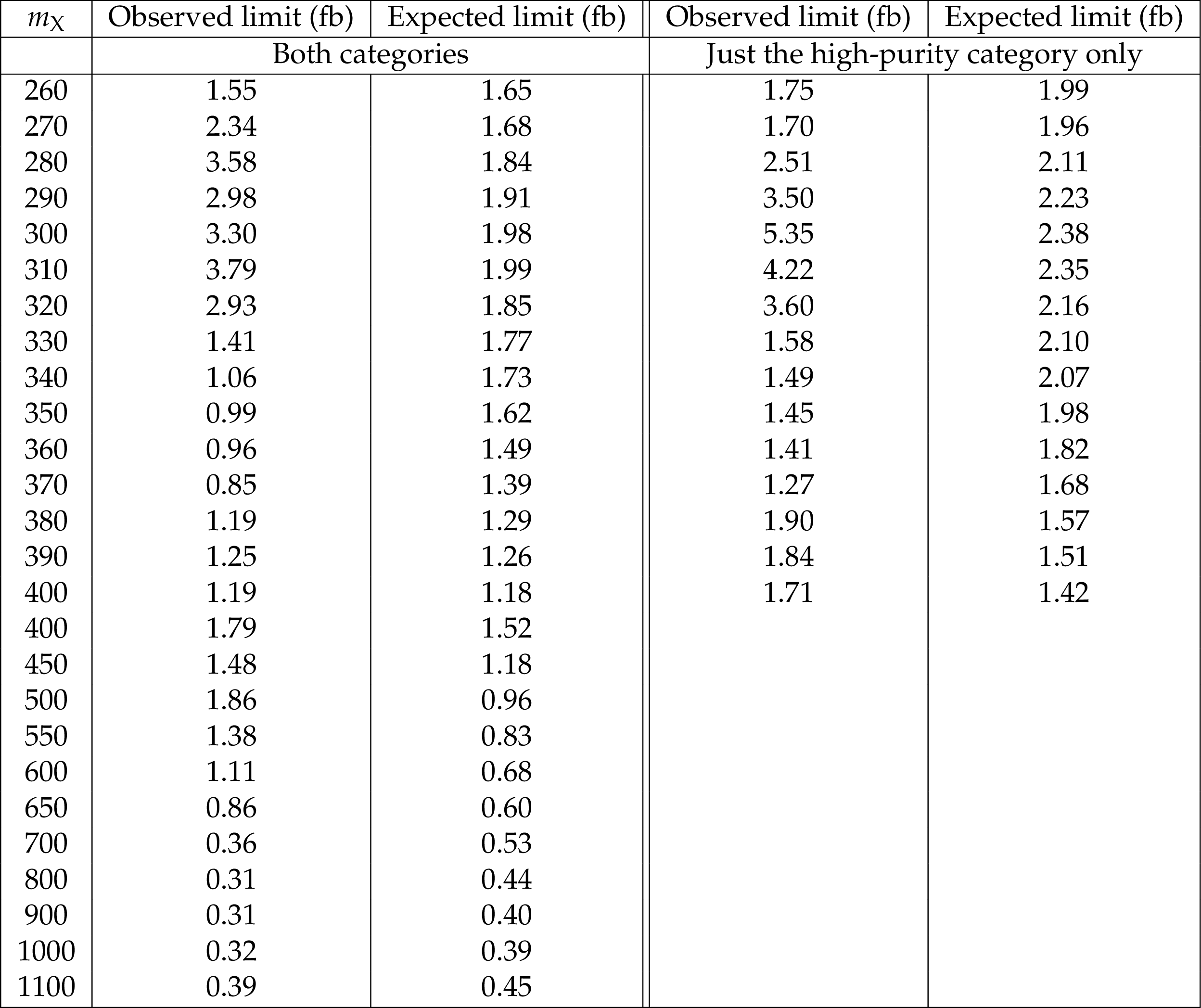
Additional Table 1:
Observed and expected median 95% CL limit from the low-mass ($ {m_\mathrm {X}} \leq$ 400 GeV) and high-mass regions ($ {m_\mathrm {X}} \geq $ 400 GeV). |
png pdf |
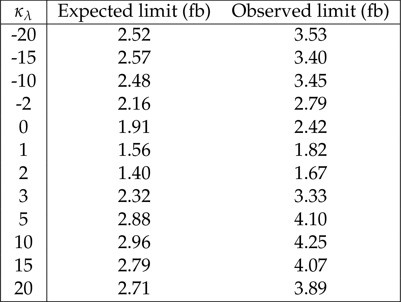
Additional Table 2:
Expected and observed 95% upper limits in fb for different assumptions about the nonresonant new physics when $ {c_2} =$ 0 and $ {\kappa _{\mathrm{ t } }} = $ 1. |
|
|
Compact Muon Solenoid LHC, CERN |
|

|

|

|

|

|