

Compact Muon Solenoid
LHC, CERN
| CMS-HIG-14-004 ; CERN-PH-EP-2015-121 | ||
| Search for the standard model Higgs boson produced through vector boson fusion and decaying to $\mathrm{ b \bar{b} }$ | ||
| CMS Collaboration | ||
| 2 June 2015 | ||
| Phys. Rev. D 92 (2015) 032008 | ||
| Abstract: A first search is reported for a standard model Higgs boson (H) that is produced through vector boson fusion and decays to a bottom-quark pair. Two data samples, corresponding to integrated luminosities of 19.8 fb$^{-1}$ and 18.3 fb$^{-1}$ of proton-proton collisions at $\sqrt{s} =$ 8 TeV were selected for this channel at the CERN LHC. The observed significance in these data samples for a $ \mathrm{ H \to b\bar{b} }$ signal at a mass of 125 GeV is 2.2 standard deviations, whilst the expected significance is 0.8 standard deviations. The fitted signal strength $\mu=\sigma/\sigma_\mathrm{SM}= 2.8 ^{+1.6}_{-1.4}$. The combination of this result with other CMS searches for the Higgs boson decaying to a b-quark pair, yields a signal strength of 1.0 $\pm$ 0.4, corresponding to a signal significance of 2.6 standard deviations for a Higgs boson mass of 125 GeV. | ||
| Links: e-print arXiv:1506.01010 [hep-ex] (PDF) ; CDS record ; inSPIRE record ; CADI line (restricted) ; | ||
| Figures | |
png pdf |
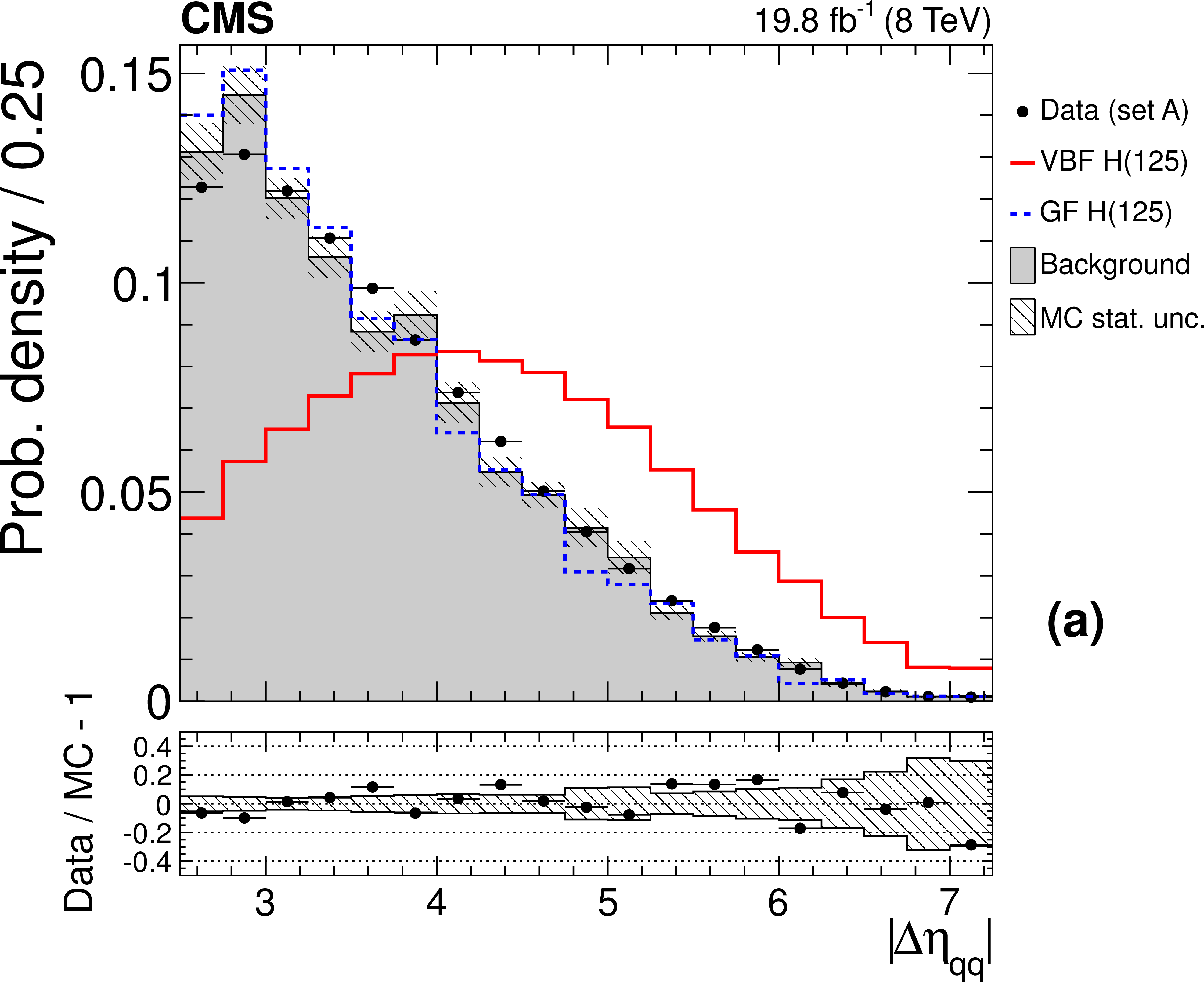
Figure 1-a:
(a) Normalized distribution in absolute pseudorapidity difference between the two VBF-jet candidates $( {| \Delta \eta _{ {\mathrm {q}} {\mathrm {q}} } | })$. (b) Normalized distribution of the azimuthal difference between the two b-jet candidates $(\Delta \phi _{ {\mathrm {b}} {\mathrm {b}} })$. The selection corresponds to set A, data are shown by the points, and the sum of all simulated backgrounds is by the filled histograms. The VBF Higgs boson signal is displayed by a solid line, and the GF Higgs boson signal is shown by a dashed line. The panels at the bottom show the fractional difference between data and background simulation, with the shaded band representing the statistical uncertainties in the MC samples. |

png pdf |
Figure 1-b:
(a) Normalized distribution in absolute pseudorapidity difference between the two VBF-jet candidates $( {| \Delta \eta _{ {\mathrm {q}} {\mathrm {q}} } | })$. (b) Normalized distribution of the azimuthal difference between the two b-jet candidates $(\Delta \phi _{ {\mathrm {b}} {\mathrm {b}} })$. The selection corresponds to set A, data are shown by the points, and the sum of all simulated backgrounds is by the filled histograms. The VBF Higgs boson signal is displayed by a solid line, and the GF Higgs boson signal is shown by a dashed line. The panels at the bottom show the fractional difference between data and background simulation, with the shaded band representing the statistical uncertainties in the MC samples. |
png pdf |
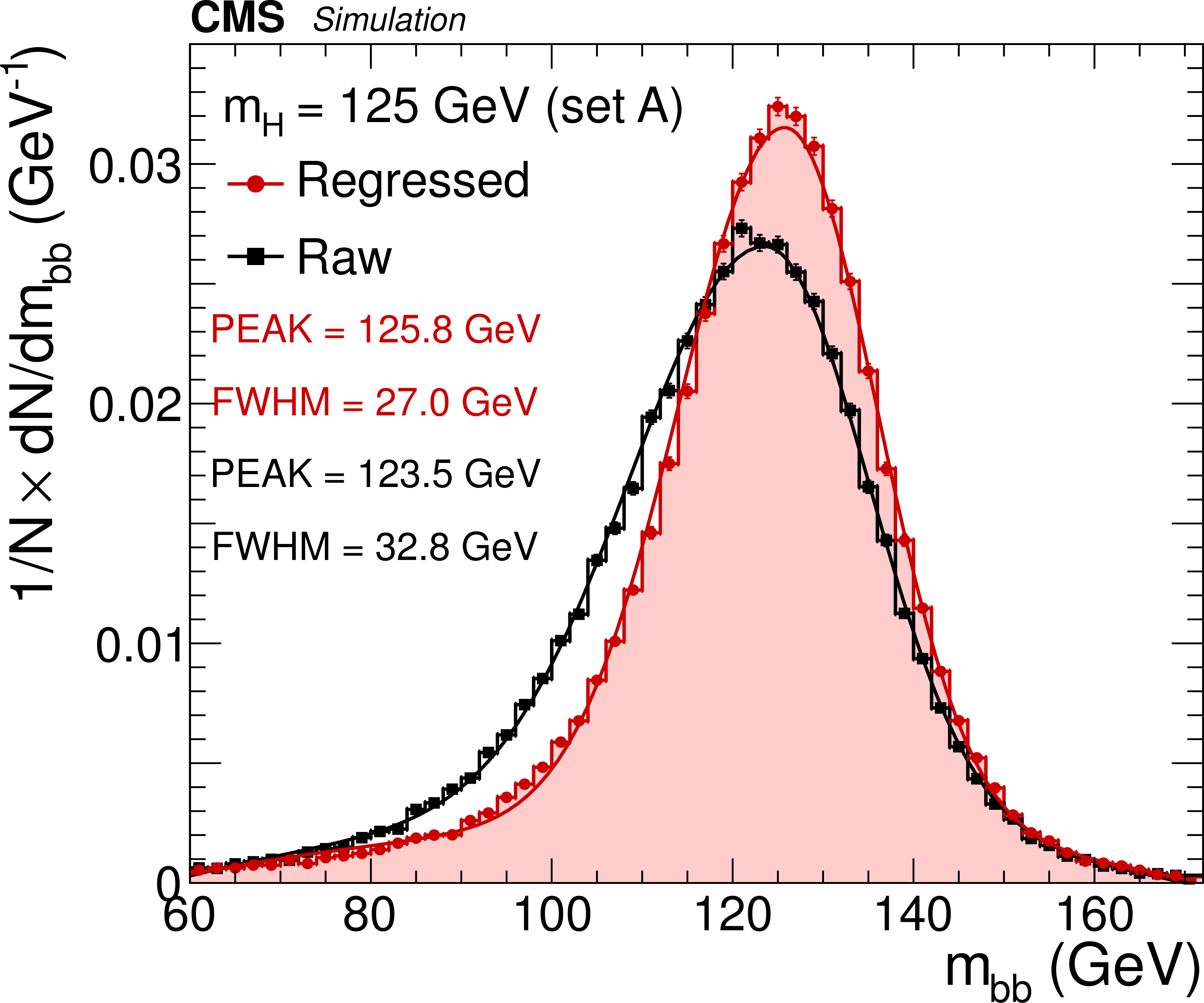
Figure 2:
Simulated invariant mass distribution of the two b-jet candidates before and after the jet $ {p_{\mathrm {T}}} $ regression, for VBF signal events. The generated Higgs boson signal mass is 125 GeV and the event selection corresponds to set A. By FWHM we denote the width of the distribution at the middle of its maximum height. |
png pdf |
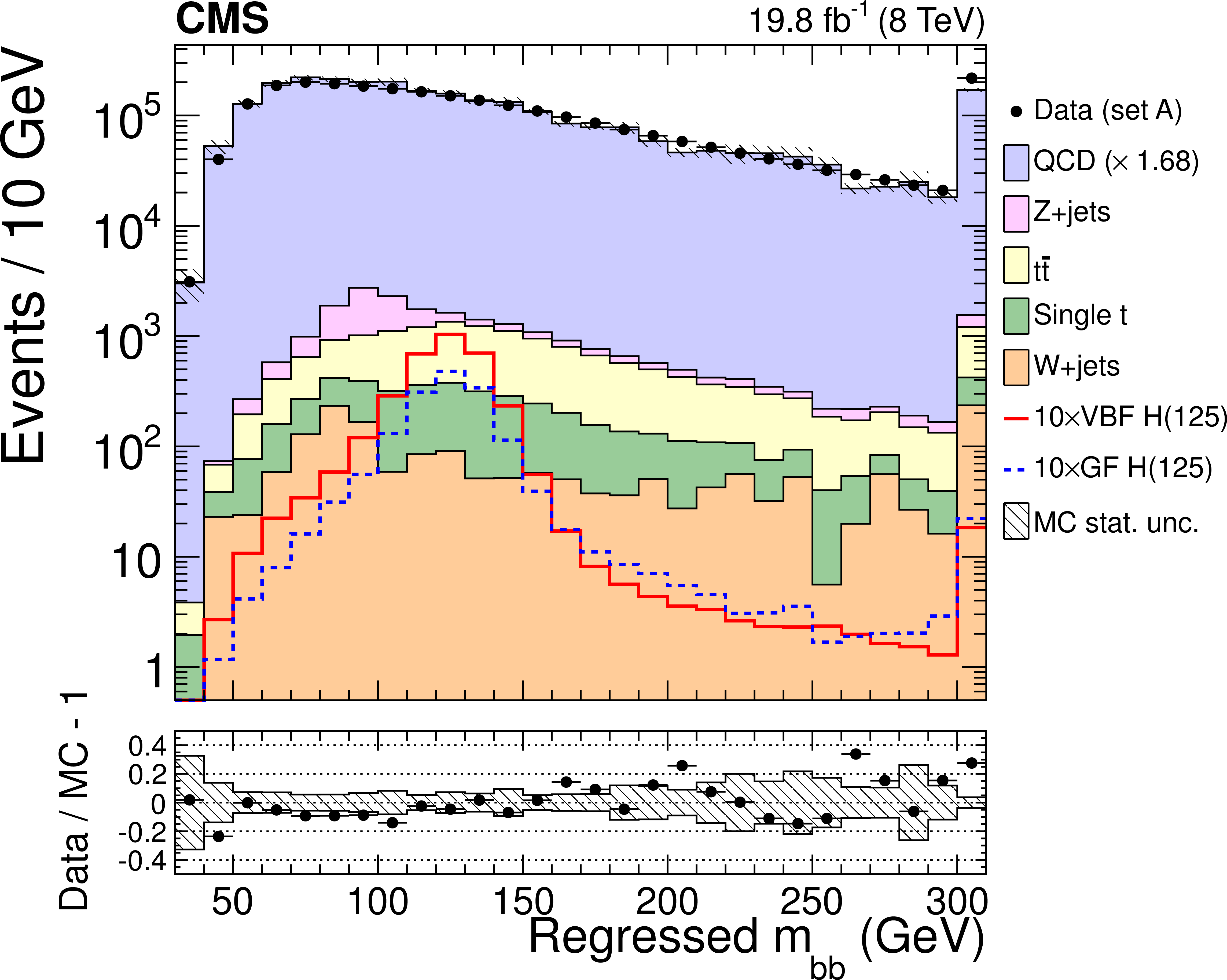
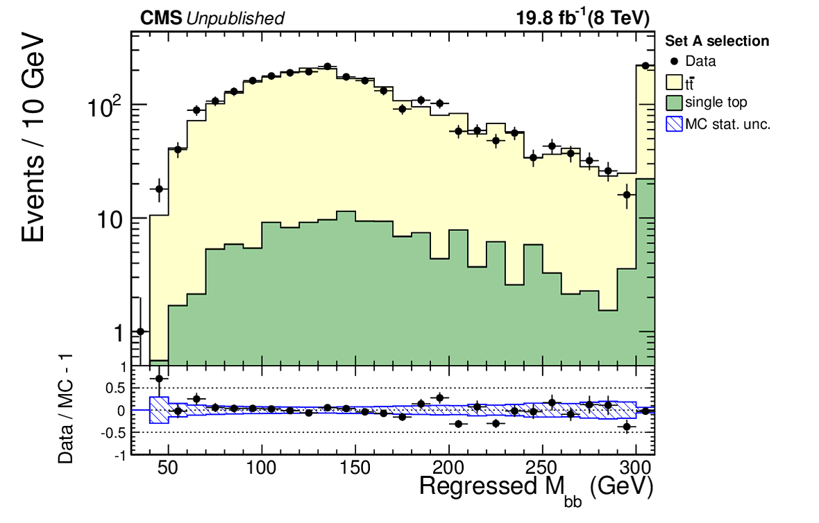
Figure 3:
Distribution in invariant mass of the two b-jet candidates, after the jet $ {p_{\mathrm {T}}} $ regression, for the events of set A. Data are shown by the points, while the simulated backgrounds are stacked. The LO QCD cross section is multiplied by a factor $1.68$ so that the total number of background events equals the number of events in the data, while the VBF and GF Higgs boson signal cross sections are multiplied by a factor 10 for better visibility. The last bin is the sum of all the events beyond the range of the $x$ axis (overflow). The panel at the bottom shows the fractional difference between data and background simulation, with the shaded band representing the statistical uncertainties in the MC samples. |
png pdf |
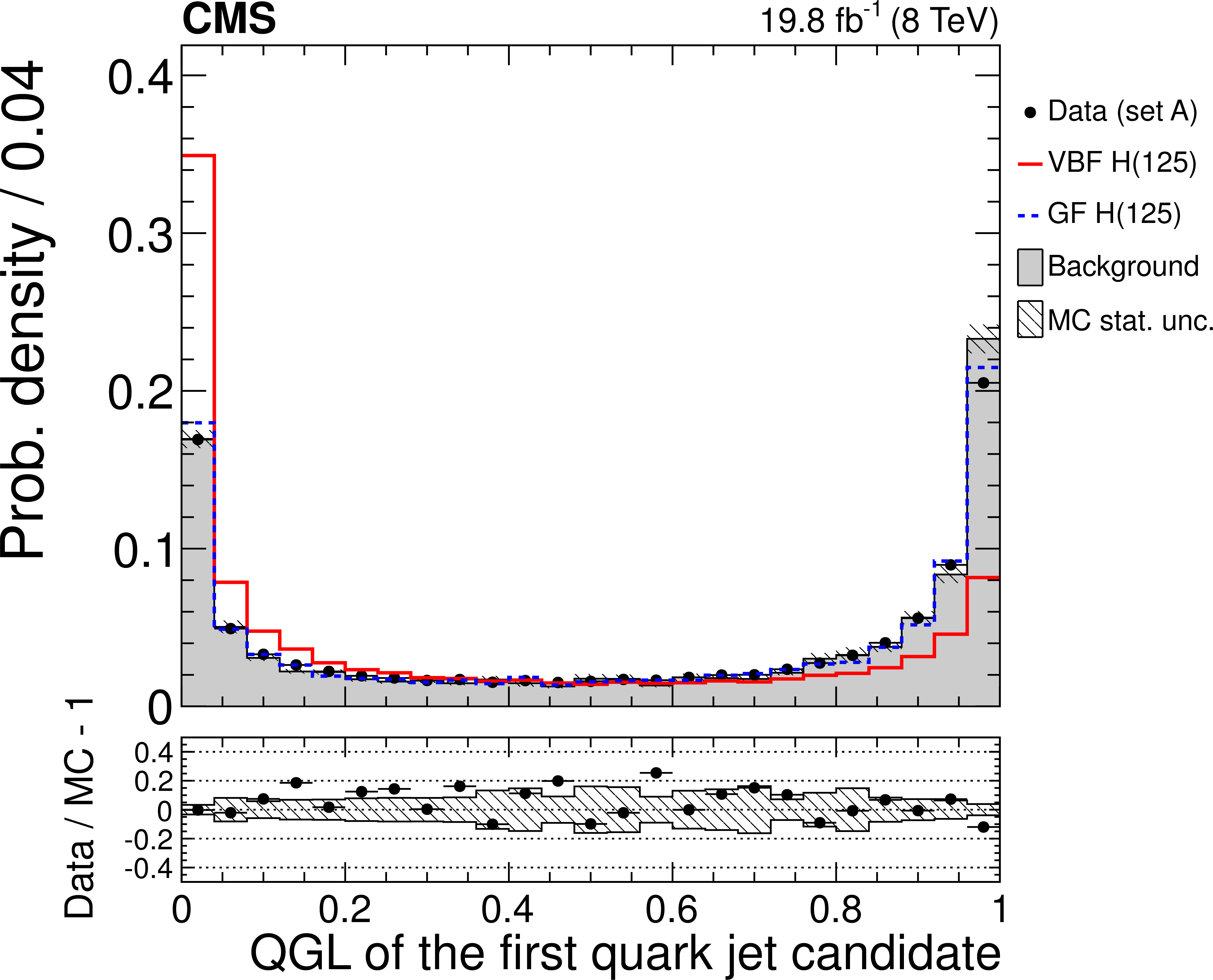
Figure 4:
Normalized distribution in quark-gluon likelihood discriminant of the first light-jet candidate. Quark jets are expected to have low likelihood values (closer to 0), while gluon jets are expected to have higher ones (closer to 1). The selection corresponds to set A, data are shown by the points, and the sum of all simulated backgrounds is shown by the filled histogram. The VBF Higgs boson signal is displayed by a solid line, and the GF Higgs boson signal is shown by a dashed line. The panel at the bottom shows the fractional difference between data and background simulation, with the shaded band representing the statistical uncertainties in the MC samples. |
png pdf |
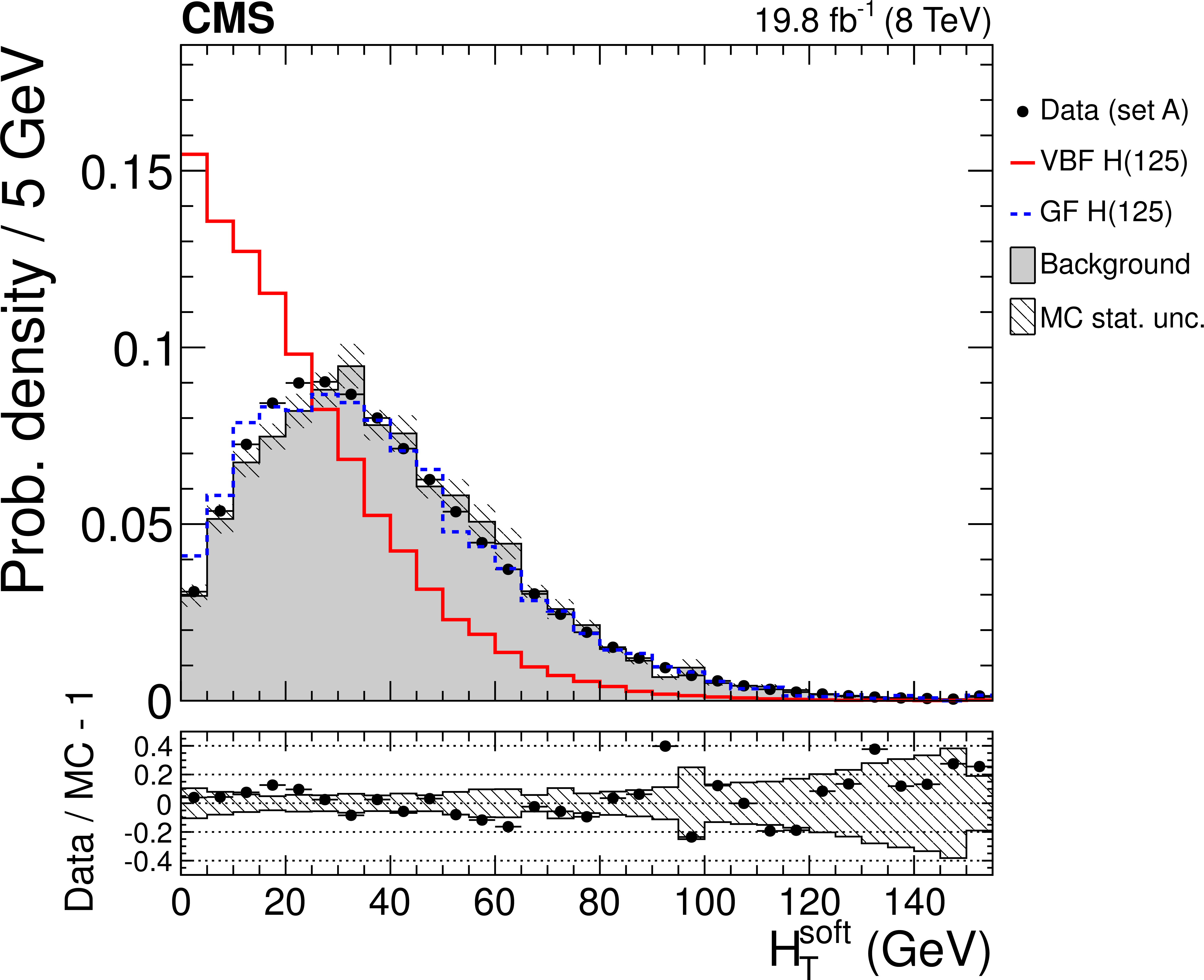
Figure 5:
Normalized distribution in scalar $ {p_{\mathrm {T}}} $ sum of TrackJets that are associated with the soft QCD activity $( {H_{\mathrm {T}}} ^\text {soft})$. The selection corresponds to set A, data are shown by the points, and the sum of all simulated backgrounds is shown by the filled histogram. The VBF Higgs boson signal is displayed by solid line, and the GF Higgs boson signal is shown by dashed line. The panel at the bottom shows the fractional difference between data and background simulation, with the shaded band representing the statistical uncertainties in the MC samples. |
png pdf |
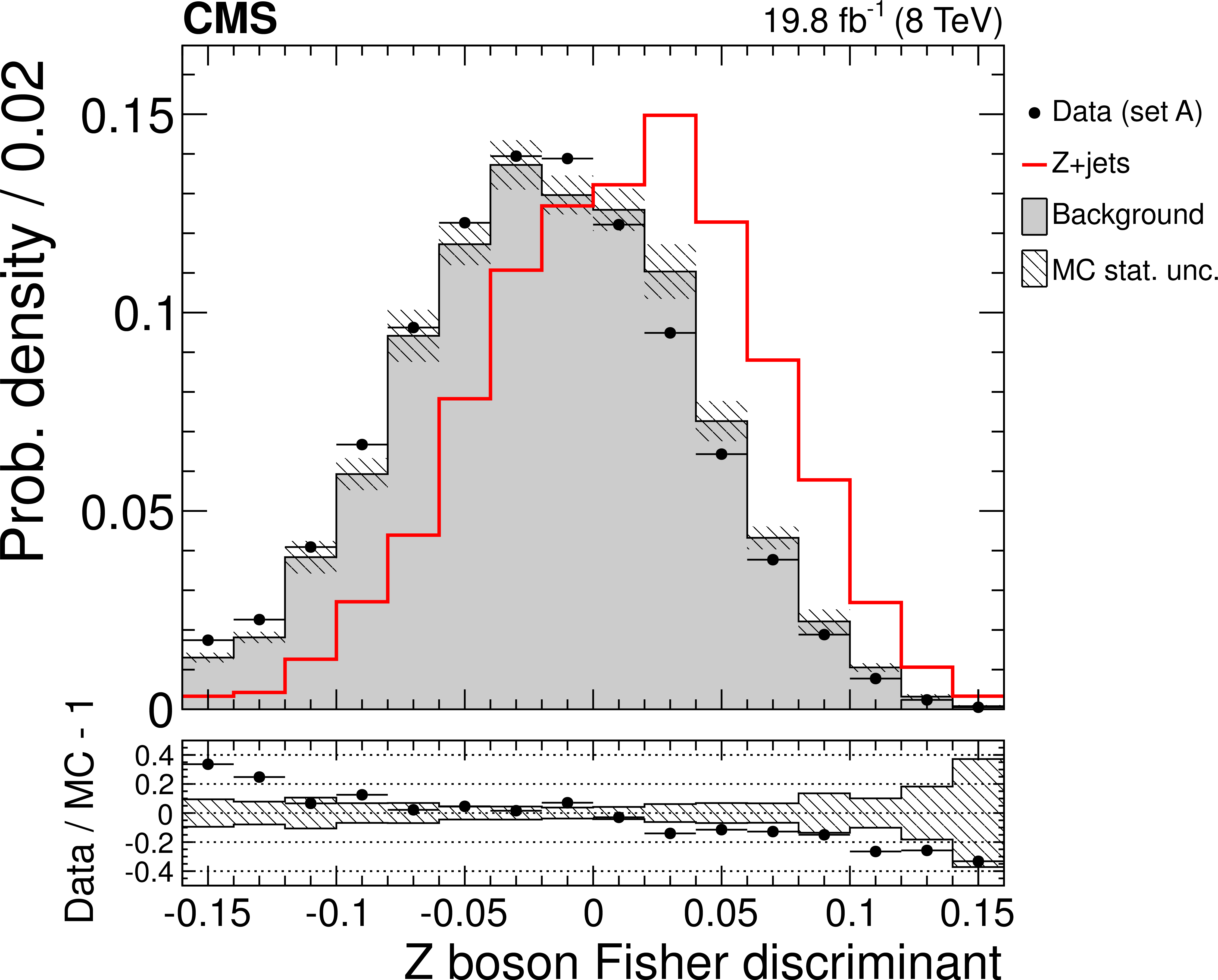
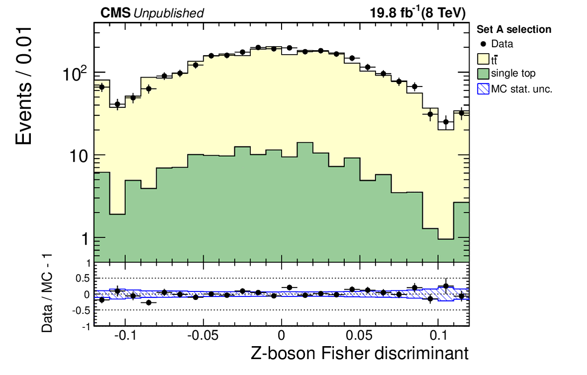
Figure 6:
Normalized distribution in $ {\mathrm {Z}} $ boson Fisher discriminant. Data are shown by the points, and the sum of all simulated backgrounds is shown by the filled histogram. The Z+jets signal is displayed with solid line. The panel at the bottom shows the fractional difference between data and background simulation, with the shaded band representing the statistical uncertainties in the MC samples. |

png pdf |
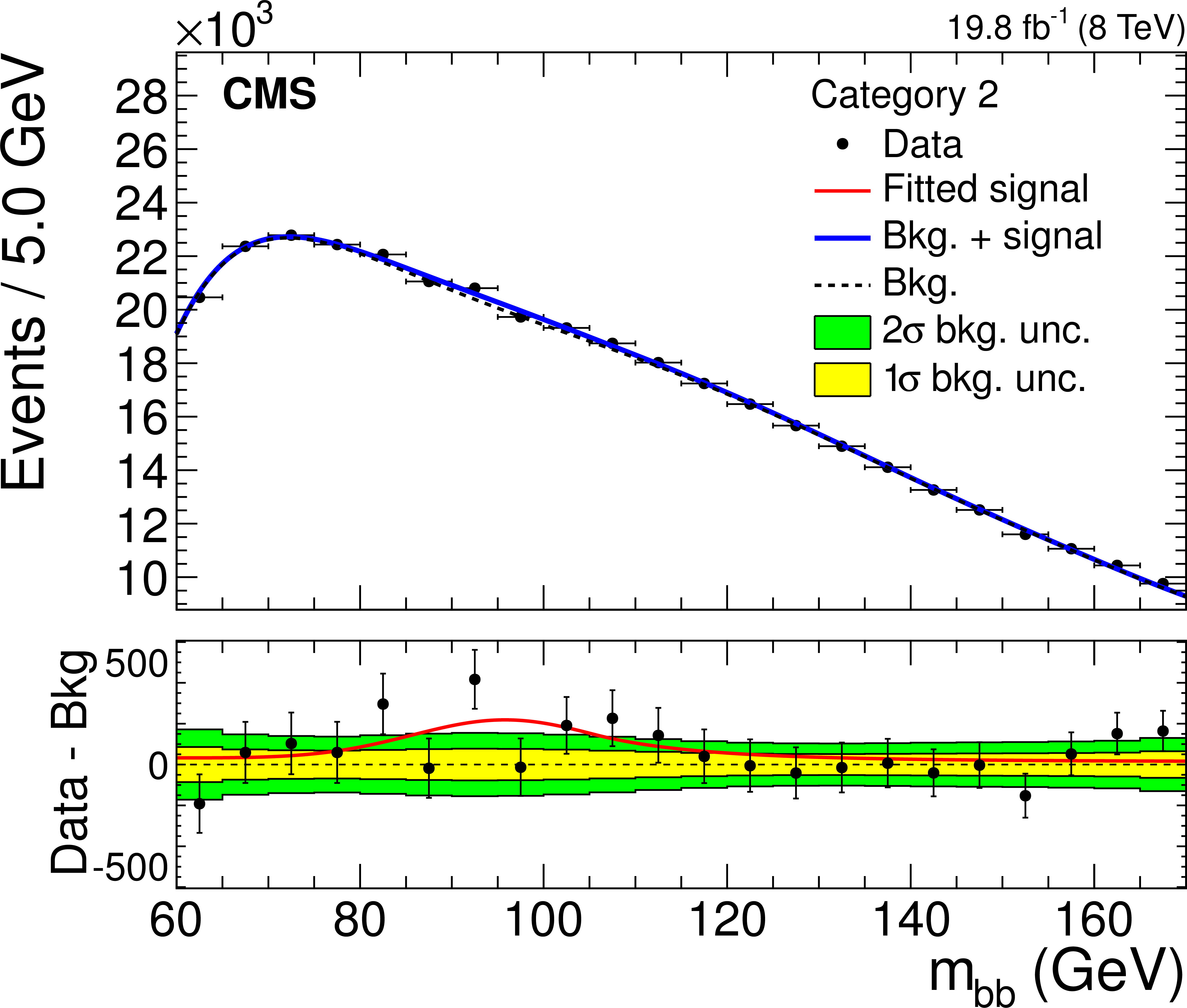
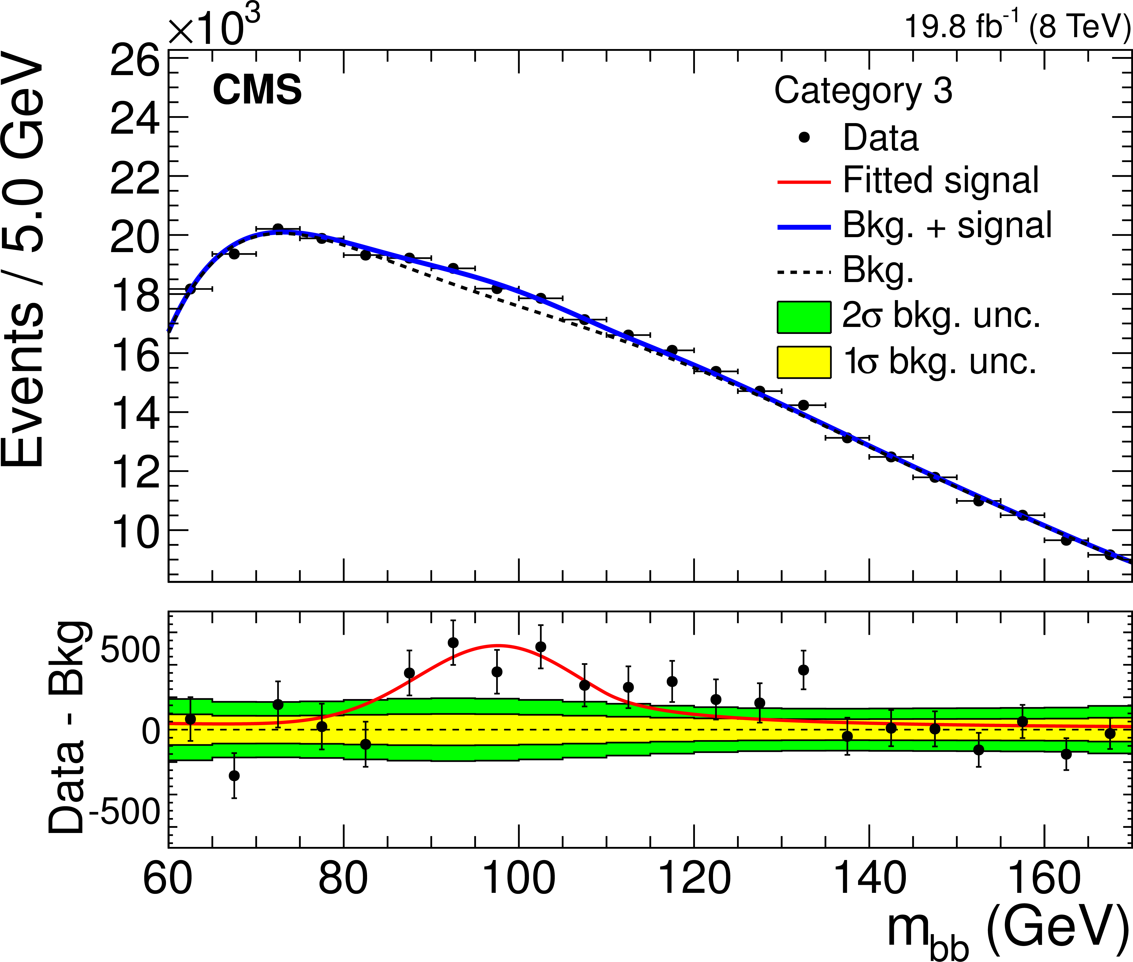
Figure 7-a:
Invariant mass distribution of the two b-jet candidates for the Z boson signal, in the three event categories that are based on the Z boson Fisher discriminant output, starting from the most background-like (a) and ending at the most signal-like (c). Data are shown by the points. The solid line is the sum of the post-fit background and signal shapes, while the dashed line is the background component alone. The bottom panel shows the background-subtracted distribution, overlaid with the fitted signal, and with the 1$\sigma $ and 2$\sigma $ background uncertainty bands. The measured (simulated) parameters of the Gaussian core of the signal shape in category 3 are 97.7 (96.6) GeV and 9.3 (9.1) GeV for the mean and the sigma, respectively. |
png pdf |
Figure 7-b:
Invariant mass distribution of the two b-jet candidates for the Z boson signal, in the three event categories that are based on the Z boson Fisher discriminant output, starting from the most background-like (a) and ending at the most signal-like (c). Data are shown by the points. The solid line is the sum of the post-fit background and signal shapes, while the dashed line is the background component alone. The bottom panel shows the background-subtracted distribution, overlaid with the fitted signal, and with the 1$\sigma $ and 2$\sigma $ background uncertainty bands. The measured (simulated) parameters of the Gaussian core of the signal shape in category 3 are 97.7 (96.6) GeV and 9.3 (9.1) GeV for the mean and the sigma, respectively. |
png pdf |
Figure 7-c:
Invariant mass distribution of the two b-jet candidates for the Z boson signal, in the three event categories that are based on the Z boson Fisher discriminant output, starting from the most background-like (a) and ending at the most signal-like (c). Data are shown by the points. The solid line is the sum of the post-fit background and signal shapes, while the dashed line is the background component alone. The bottom panel shows the background-subtracted distribution, overlaid with the fitted signal, and with the 1$\sigma $ and 2$\sigma $ background uncertainty bands. The measured (simulated) parameters of the Gaussian core of the signal shape in category 3 are 97.7 (96.6) GeV and 9.3 (9.1) GeV for the mean and the sigma, respectively. |
png pdf |
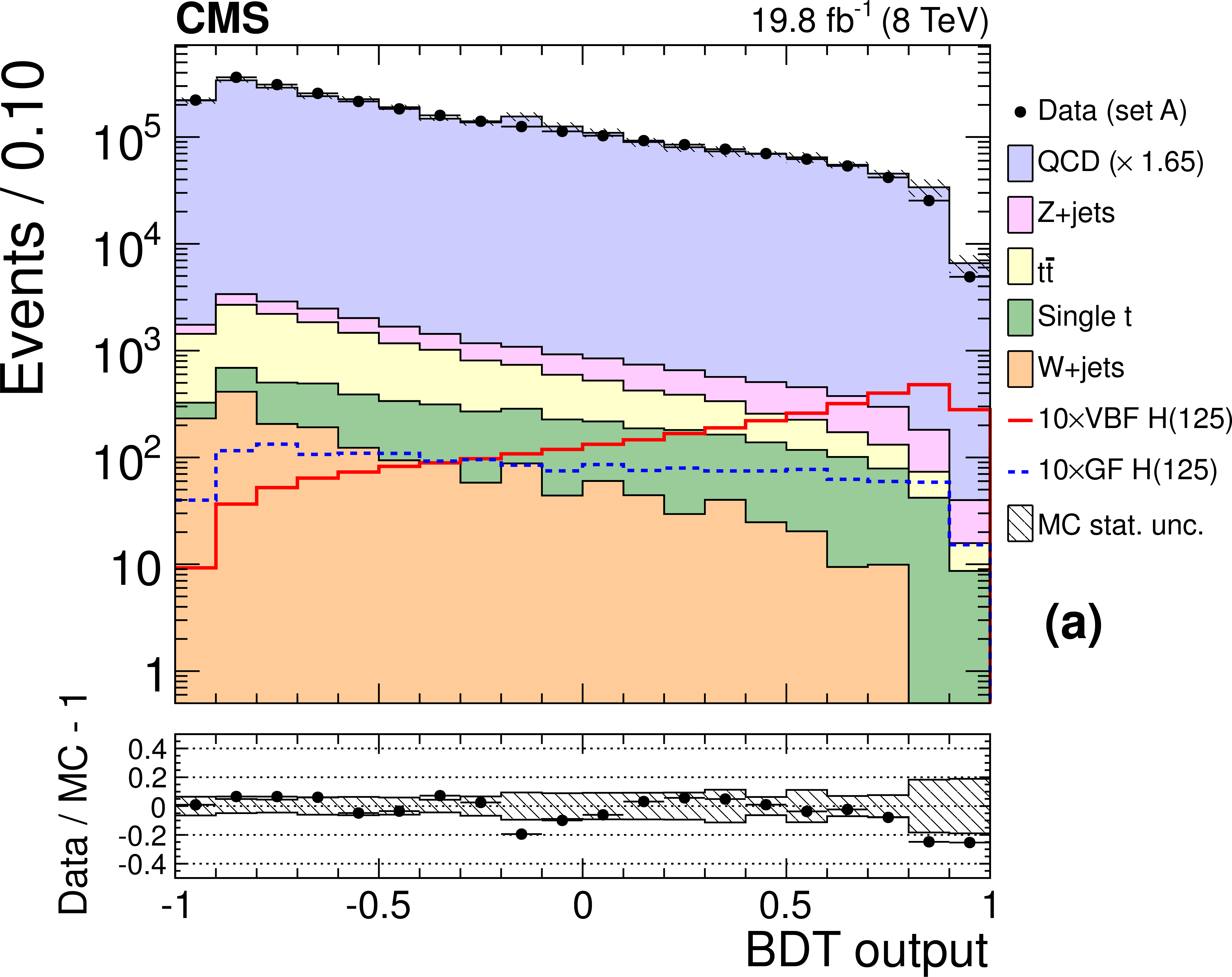
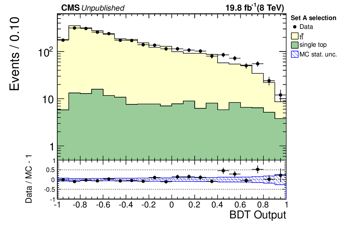
Figure 8-a:
Distribution of the BDT output for the events of set A (a) and set B (b). Data are shown by the points, while the simulated backgrounds are stacked. The LO QCD cross sections are scaled such that the total number of background events equals the number of events in data, while the VBF and GF Higgs boson signal yields are multiplied by a factor of 10 for better visibility. The panels at the bottom show the fractional difference between data and background simulation, with the shaded band representing the statistical uncertainties of the MC samples. |
png pdf |
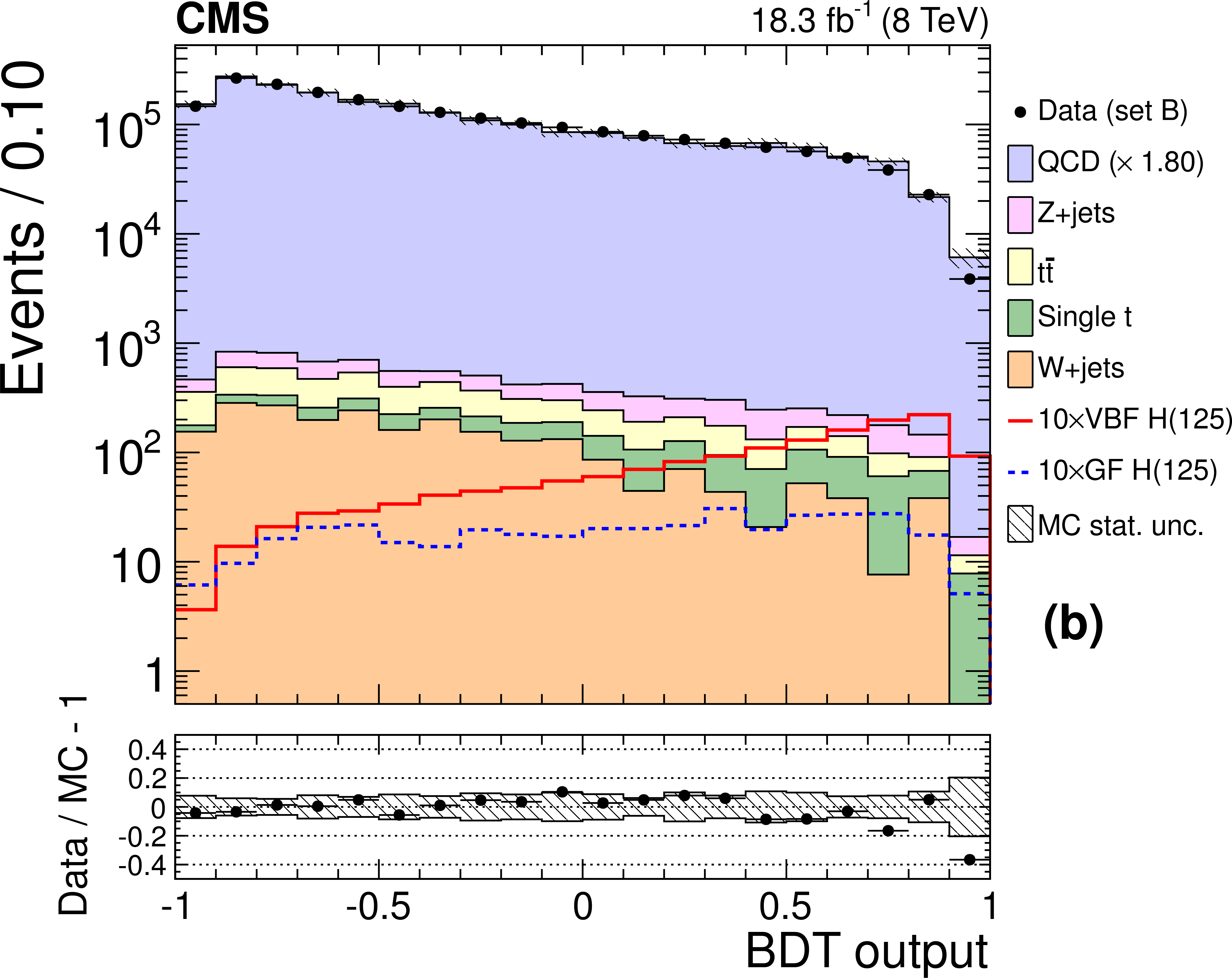
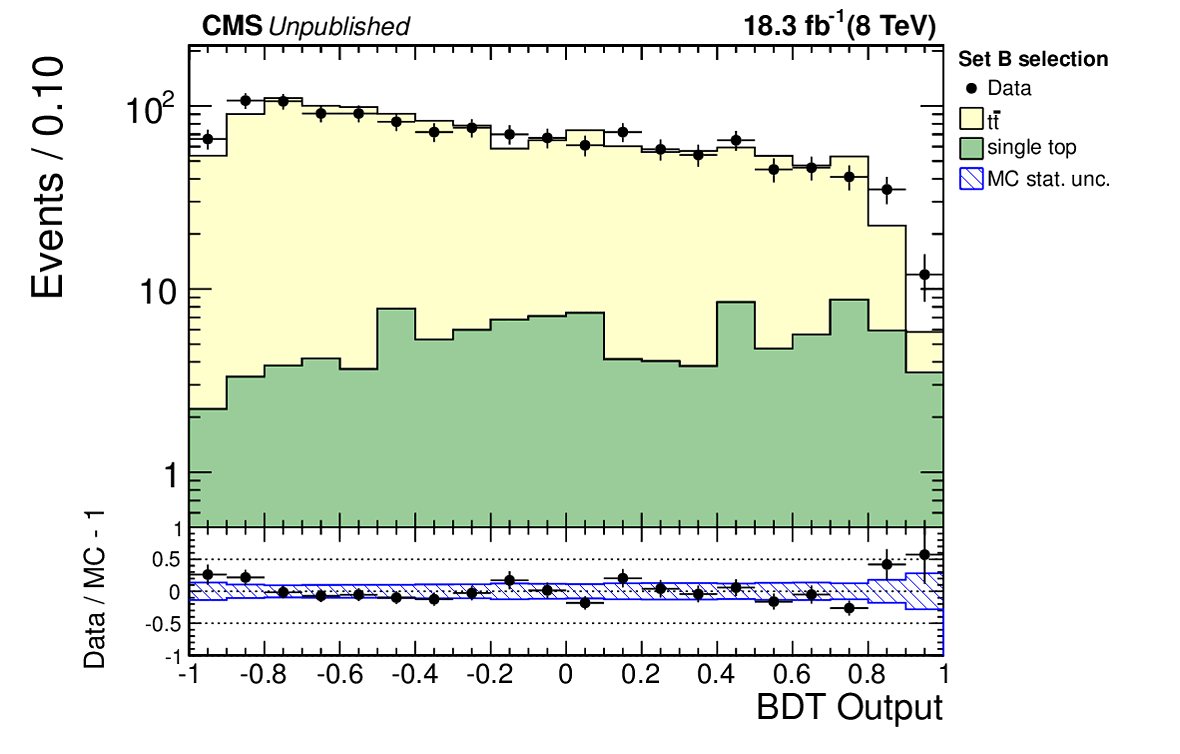
Figure 8-b:
Distribution of the BDT output for the events of set A (a) and set B (b). Data are shown by the points, while the simulated backgrounds are stacked. The LO QCD cross sections are scaled such that the total number of background events equals the number of events in data, while the VBF and GF Higgs boson signal yields are multiplied by a factor of 10 for better visibility. The panels at the bottom show the fractional difference between data and background simulation, with the shaded band representing the statistical uncertainties of the MC samples. |
png pdf |
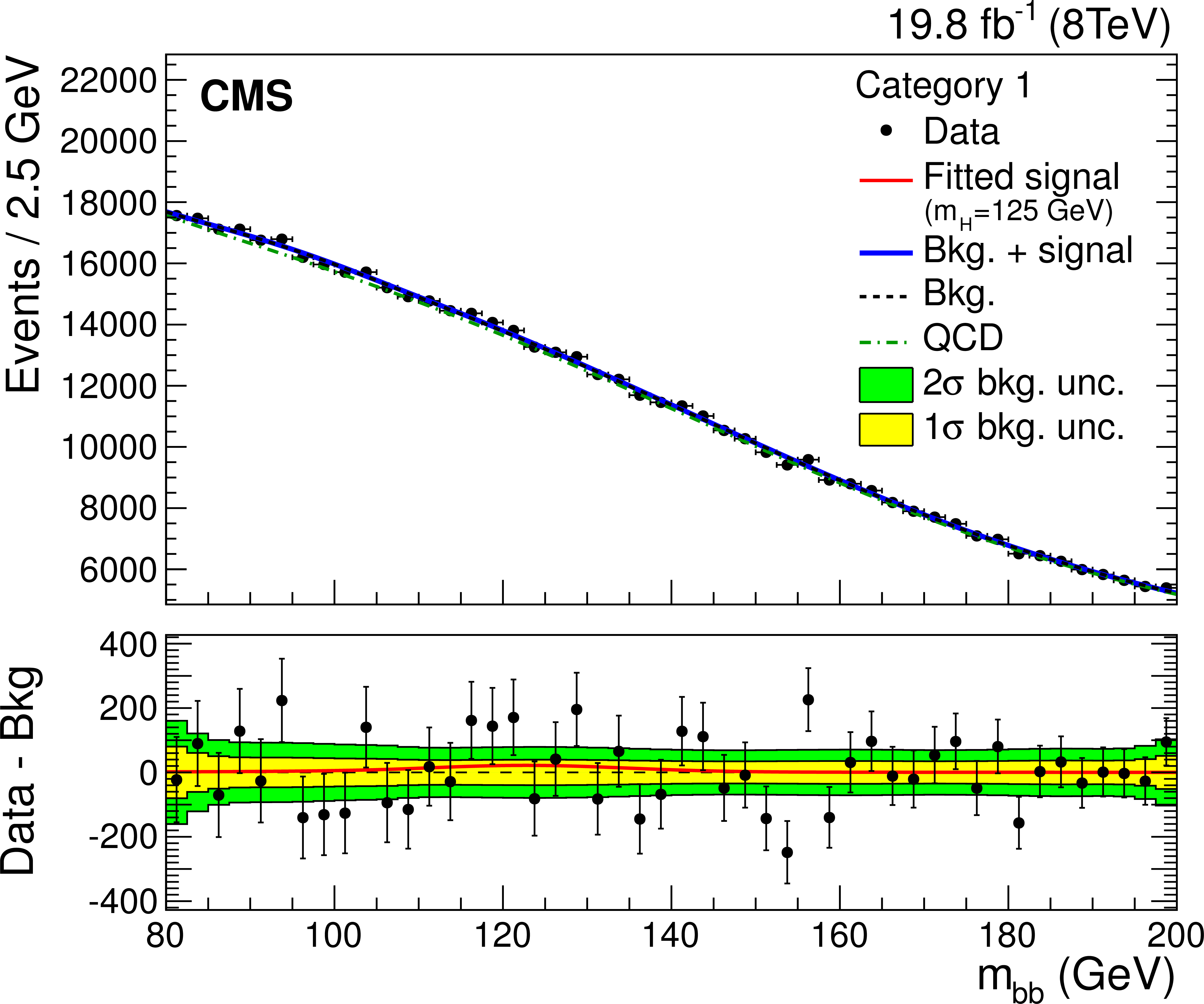
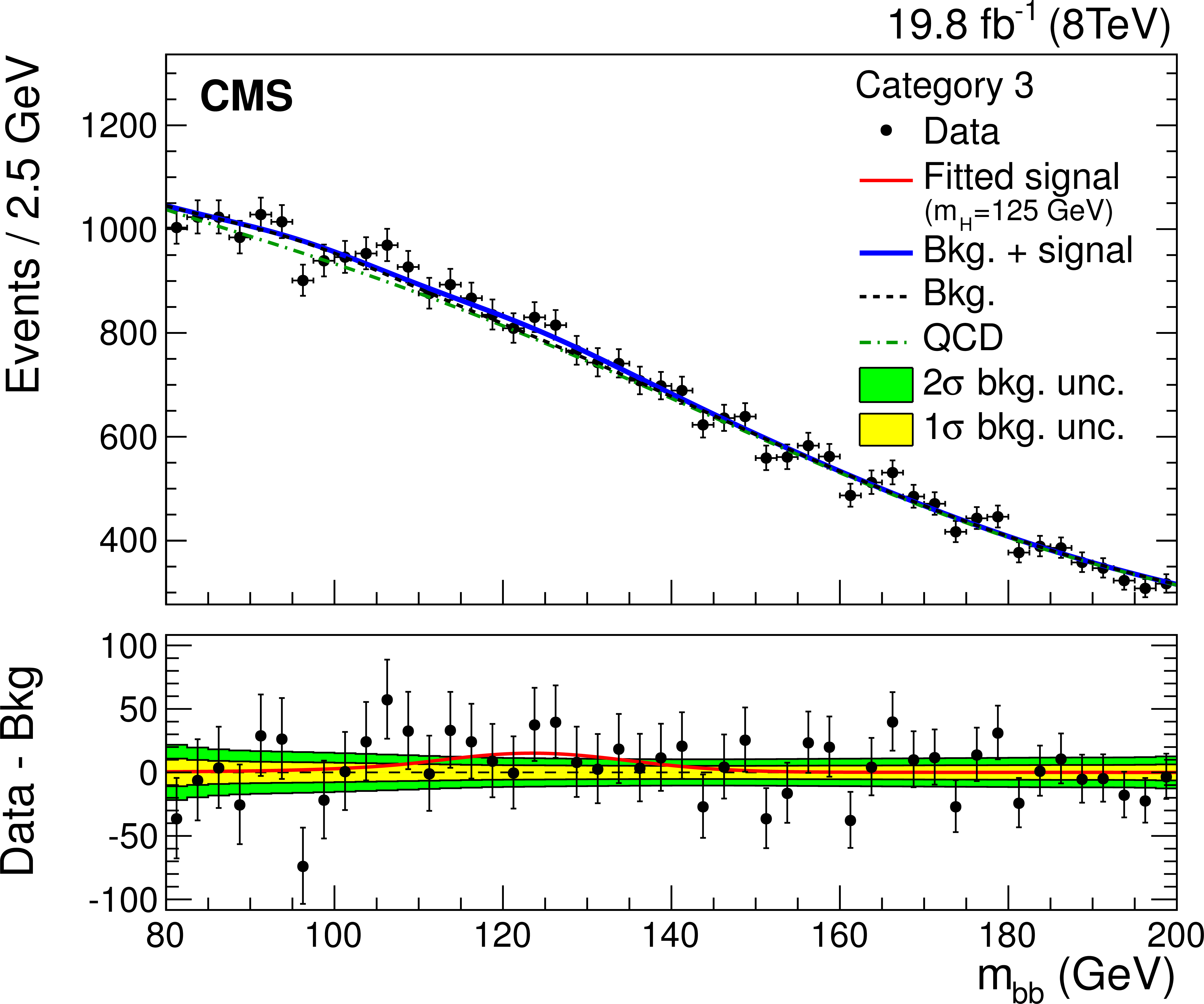
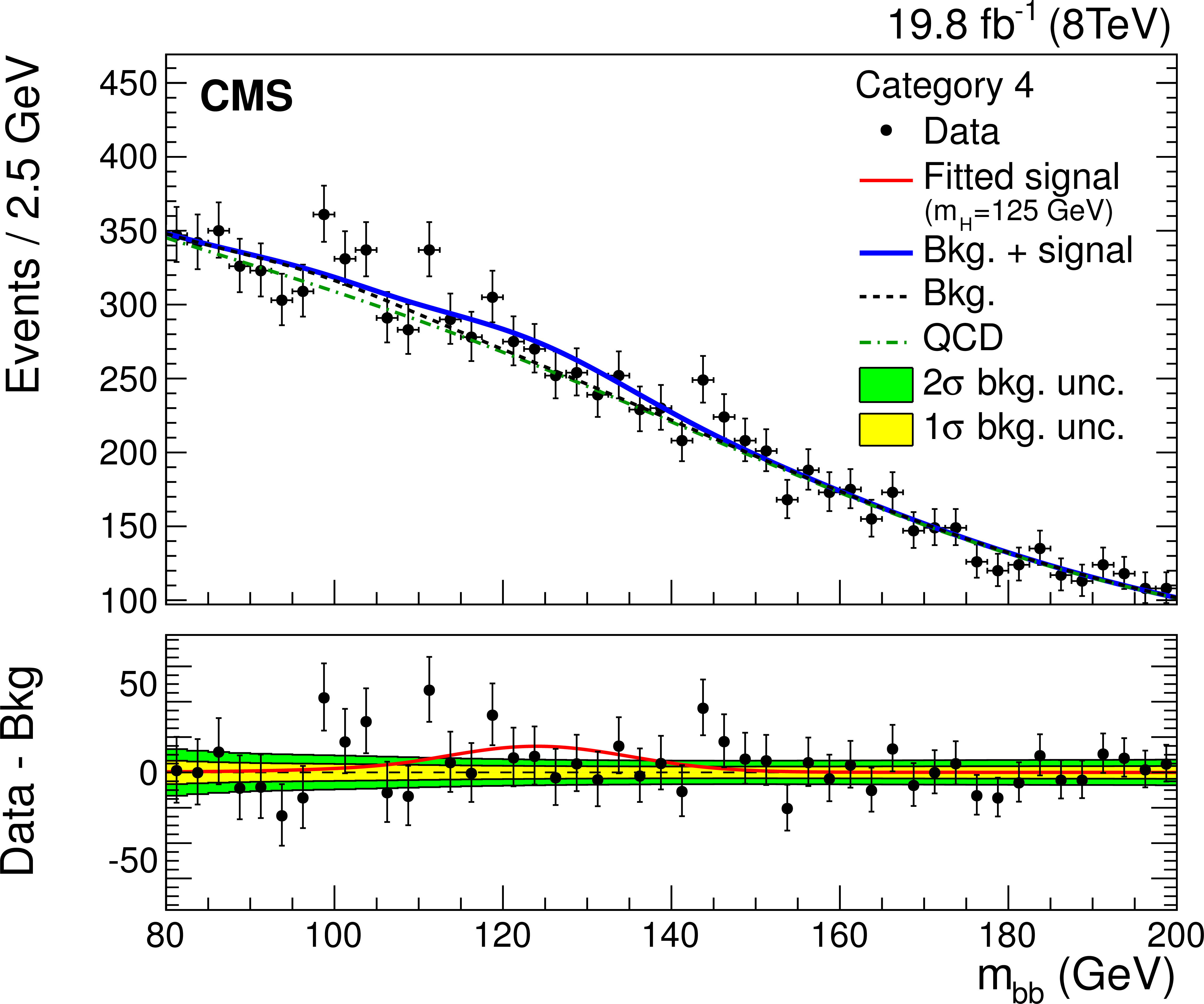
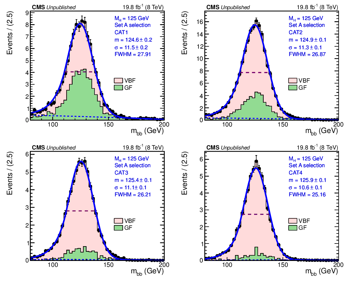
Figure 9-a:
Fit of the invariant mass of the two b-jet candidates for the Higgs boson signal ($m_{ {\mathrm {H}} }=$ 125 GeV) in the four event categories of set A. Data are shown by the points. The solid line is the sum of the post-fit background and signal shapes, the dashed line is the background component, and the dashed-dotted line is the QCD component alone. The bottom panel shows the background-subtracted distribution, overlaid with the fitted signal, and with the 1$\sigma $ and 2$\sigma $ background uncertainty bands. |
png pdf |
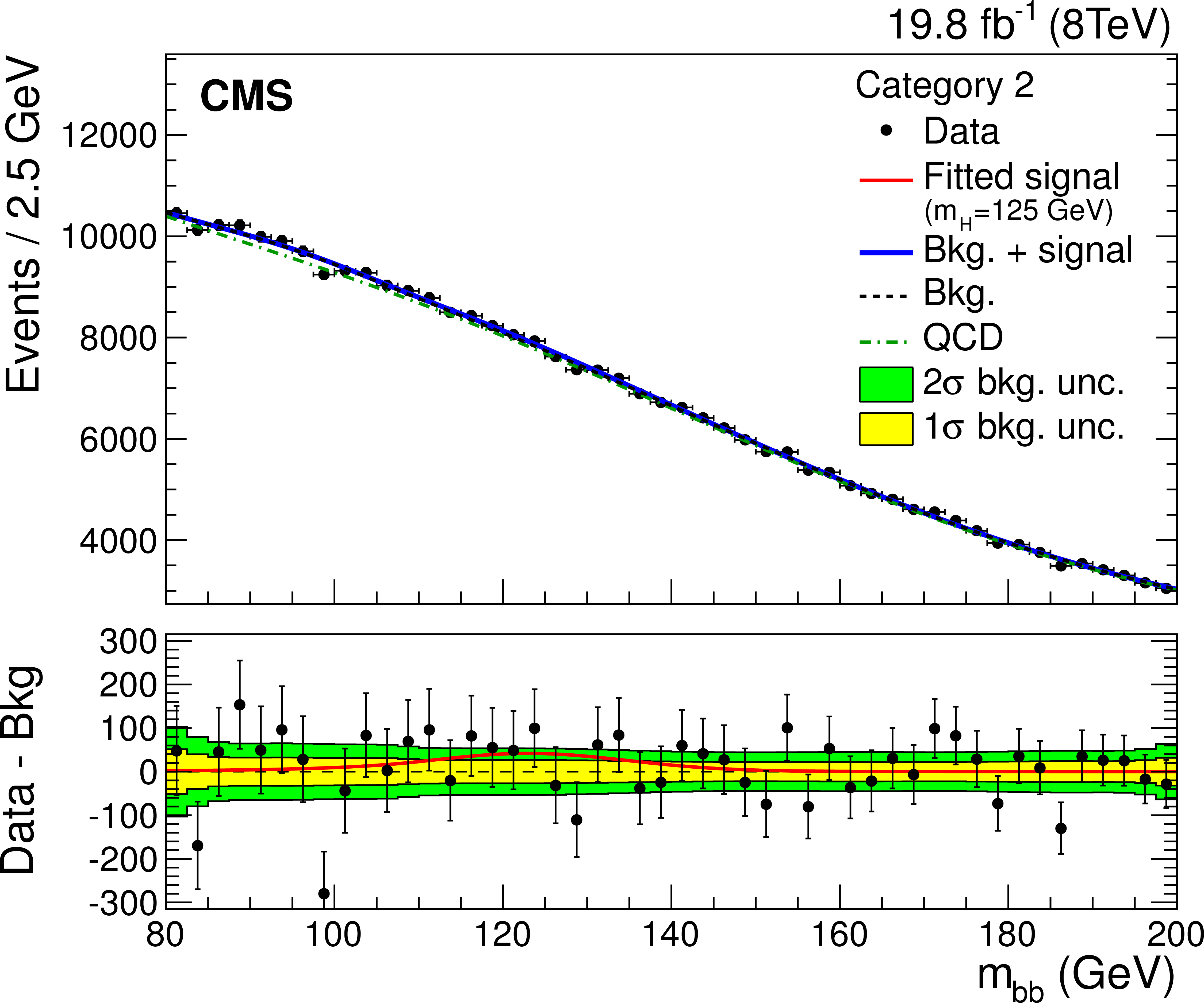
Figure 9-b:
Fit of the invariant mass of the two b-jet candidates for the Higgs boson signal ($m_{ {\mathrm {H}} }=$ 125 GeV) in the four event categories of set A. Data are shown by the points. The solid line is the sum of the post-fit background and signal shapes, the dashed line is the background component, and the dashed-dotted line is the QCD component alone. The bottom panel shows the background-subtracted distribution, overlaid with the fitted signal, and with the 1$\sigma $ and 2$\sigma $ background uncertainty bands. |
png pdf |
Figure 9-c:
Fit of the invariant mass of the two b-jet candidates for the Higgs boson signal ($m_{ {\mathrm {H}} }=$ 125 GeV) in the four event categories of set A. Data are shown by the points. The solid line is the sum of the post-fit background and signal shapes, the dashed line is the background component, and the dashed-dotted line is the QCD component alone. The bottom panel shows the background-subtracted distribution, overlaid with the fitted signal, and with the 1$\sigma $ and 2$\sigma $ background uncertainty bands. |
png pdf |
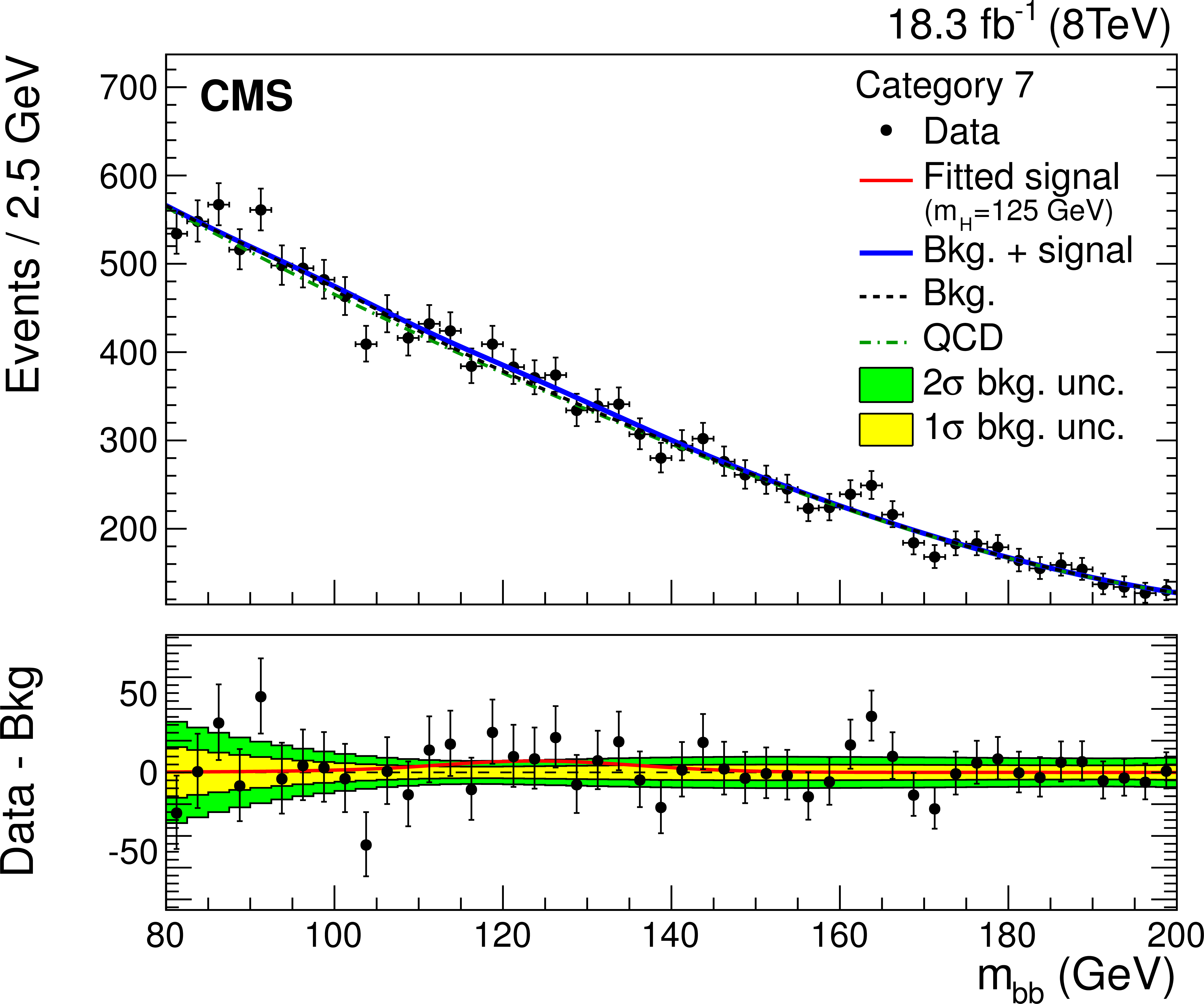
Figure 9-d:
Fit of the invariant mass of the two b-jet candidates for the Higgs boson signal ($m_{ {\mathrm {H}} }=$ 125 GeV) in the four event categories of set A. Data are shown by the points. The solid line is the sum of the post-fit background and signal shapes, the dashed line is the background component, and the dashed-dotted line is the QCD component alone. The bottom panel shows the background-subtracted distribution, overlaid with the fitted signal, and with the 1$\sigma $ and 2$\sigma $ background uncertainty bands. |
png pdf |
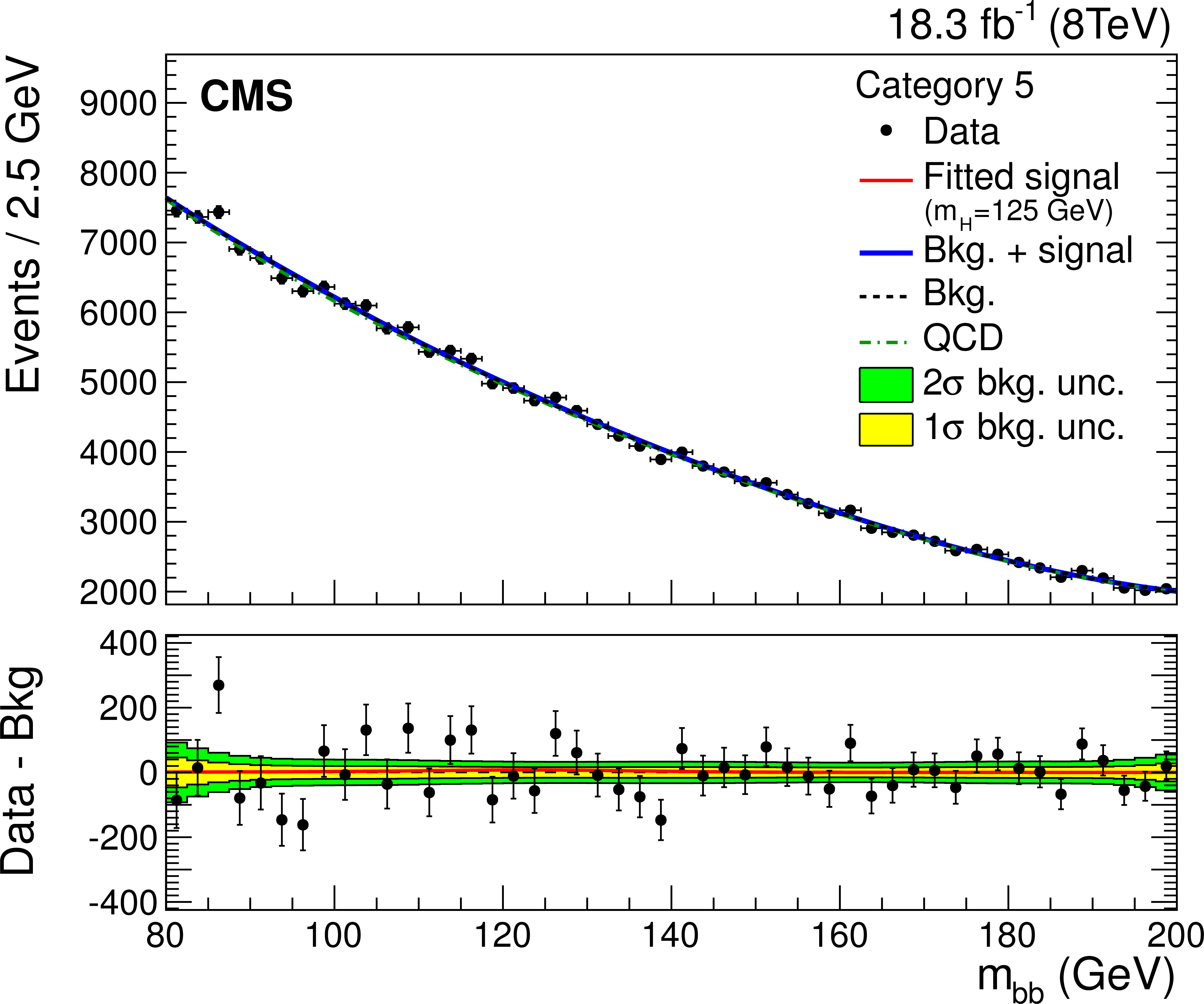
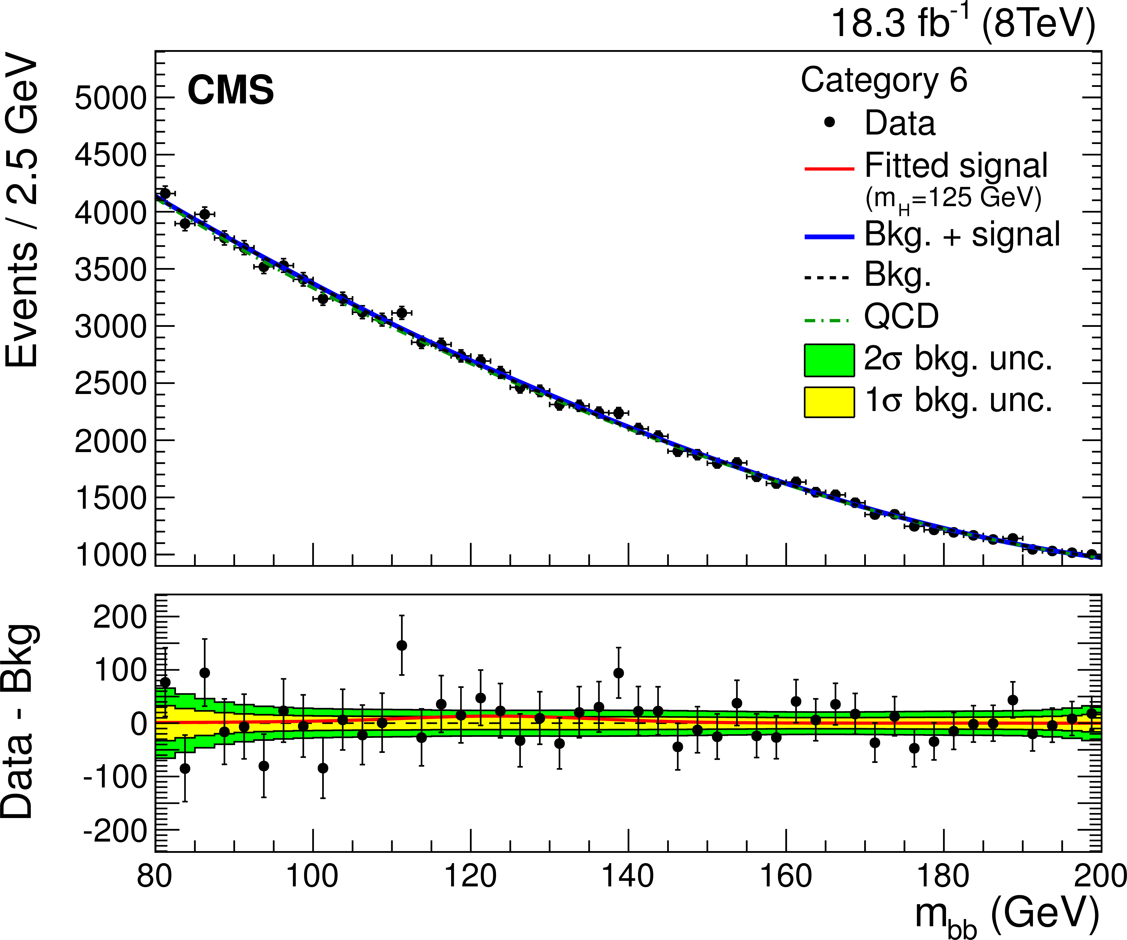
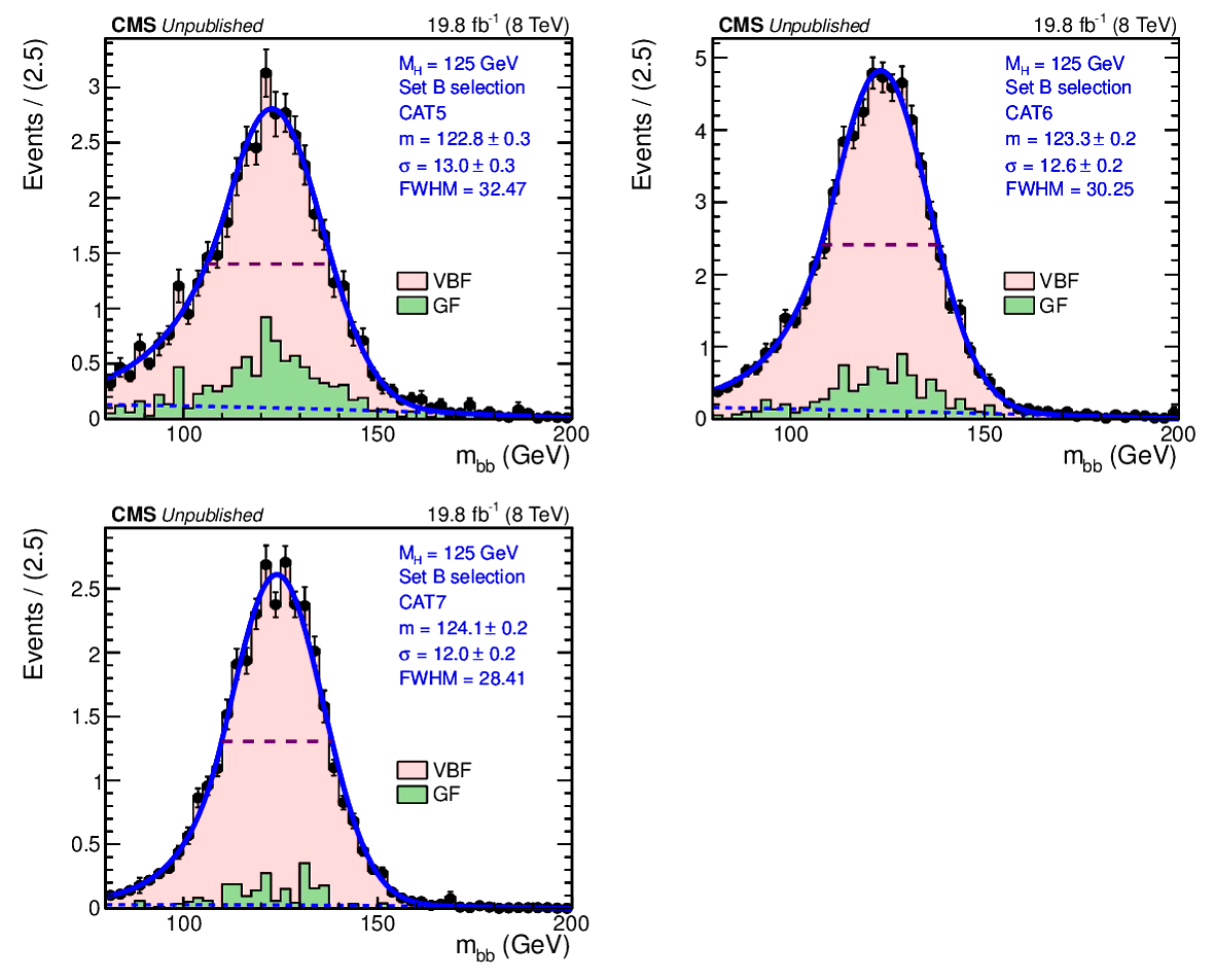
Figure 10-a:
Fit of the invariant mass of the two b-jet candidates for the Higgs boson signal ($m_{ {\mathrm {H}} }=$125 GeV) in the three event categories of set B. Data are shown with markers. The solid line is the sum of the post-fit background and signal shapes, the dashed line is the background component, and the dashed-dotted line is the QCD component alone. The bottom panel shows the background-subtracted distribution, overlaid with the fitted signal, and with the 1$\sigma $ and 2$\sigma $ background uncertainty bands. |
png pdf |
Figure 10-b:
Fit of the invariant mass of the two b-jet candidates for the Higgs boson signal ($m_{ {\mathrm {H}} }=$125 GeV) in the three event categories of set B. Data are shown with markers. The solid line is the sum of the post-fit background and signal shapes, the dashed line is the background component, and the dashed-dotted line is the QCD component alone. The bottom panel shows the background-subtracted distribution, overlaid with the fitted signal, and with the 1$\sigma $ and 2$\sigma $ background uncertainty bands. |
png pdf |
Figure 10-c:
Fit of the invariant mass of the two b-jet candidates for the Higgs boson signal ($m_{ {\mathrm {H}} }=$125 GeV) in the three event categories of set B. Data are shown with markers. The solid line is the sum of the post-fit background and signal shapes, the dashed line is the background component, and the dashed-dotted line is the QCD component alone. The bottom panel shows the background-subtracted distribution, overlaid with the fitted signal, and with the 1$\sigma $ and 2$\sigma $ background uncertainty bands. |
png pdf |
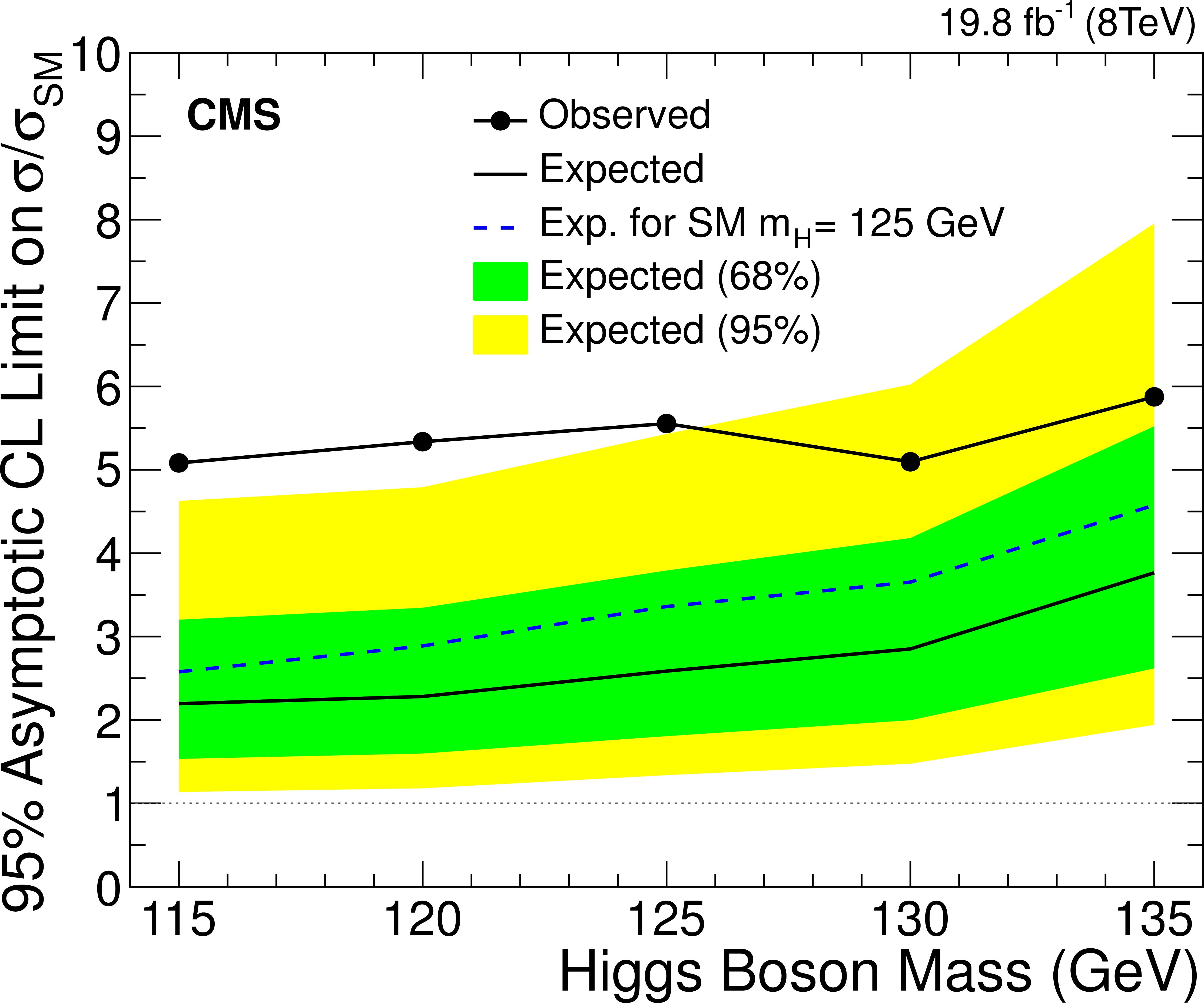
Figure 11:
Expected and observed 95% confidence level limits on the signal cross section in units of the SM expected cross section, as a function of the Higgs boson mass, including all event categories. The limits expected in the presence of a SM Higgs boson with a mass of 125 GeV are indicated by the dotted curve. |
| Tables | |
png pdf |
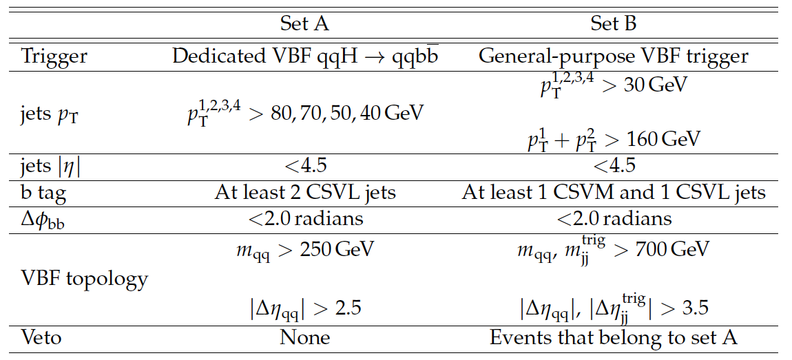
Table 1:
Summary of selection requirements for the two analyses. |

png pdf |
Table 2:
Definition of the event categories for the Z boson signal extraction and corresponding yields in the $m_{\mathcal{bb}}$ interval [60, 170] GeV. |
png pdf |
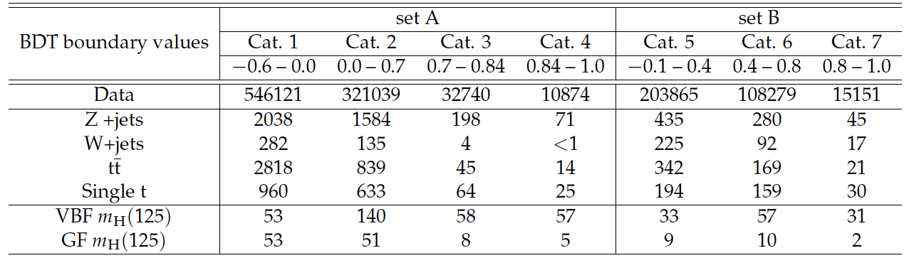
Table 3:
Definition of the event categories and corresponding yields in the $m_{\mathcal{bb}}$ interval [80, 200] GeV, for the data and the MC expectation. The BDT output boundary values refer to the distributions shown in Fig. 8. |
png pdf |
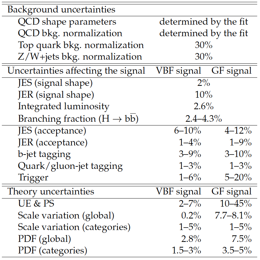
Table 4:
Sources of systematic uncertainty and their impact on the shape and normalization of the background and signal processes. |

png pdf |
Table 5:
Observed and expected 95% CL limits, best fit values on the signal strength parameter $\mu = \sigma/\sigma_{\text{SM}}$ and signal significances for $m_{\mathrm{H}} =$ 125 GeV, for each $\mathrm{ H \to b \bar{b} }$ channel and their combination. |
| Summary |
| A search has been carried out for the SM Higgs boson produced in vector boson fusion and decaying to $\mathrm{ b \bar{b} }$ with two data samples of pp collisions at $\sqrt{s} =$ 8 TeV collected with the CMS detector at the LHC corresponding to integrated luminosities of 19.8 fb$^{-1}$ and 18.3 fb$^{-1}$. Upper limits, at a 95% confidence level, on the production cross section times the $\mathrm{ H \to b \bar{b} }$ branching fraction, relative to expectations for a SM Higgs boson, are extracted for a Higgs boson in the mass range 115-135 GeV. In this range, the expected upper limits in the absence of a signal vary between a factor of 2.2 to 3.7 of the SM prediction, while the observed upper limits vary from 5.0 to 5.8. For a Higgs boson mass of 125 GeV, the observed and expected significance is, respectively, 2.2 and 0.8 standard deviations, and the fitted signal strength is $\mu = \sigma/\sigma_{\text {SM}} = 2.8 ^{+1.6}_{-1.4}$. This is the first search of this kind, and the only search for the SM Higgs boson in all-jet final states, at the LHC. The combination of the results obtained in this search with other CMS $\mathrm{ H \to b \bar{b} }$ searches in the VH and ttH production modes, yields a $\mathrm{ H \to b \bar{b} }$ signal strength $\mu = 1.03^{+0.44}_{-0.42}$ with a signal significance of 2.6 standard deviations for $m_{\mathrm{H}} =$ 125 GeV that is consistent with the SM. |
| Additional Figures | |
png pdf |
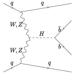
Additional Figure 1:
Lowest order Feynman diagram for the SM Higgs VBF production at the LHC. |
png pdf |
Additional Figure 2:
Cartoon showing the signal ($m_{\mathrm{H}} =$ 125 GeV) efficiency for the two selections. |
png pdf |
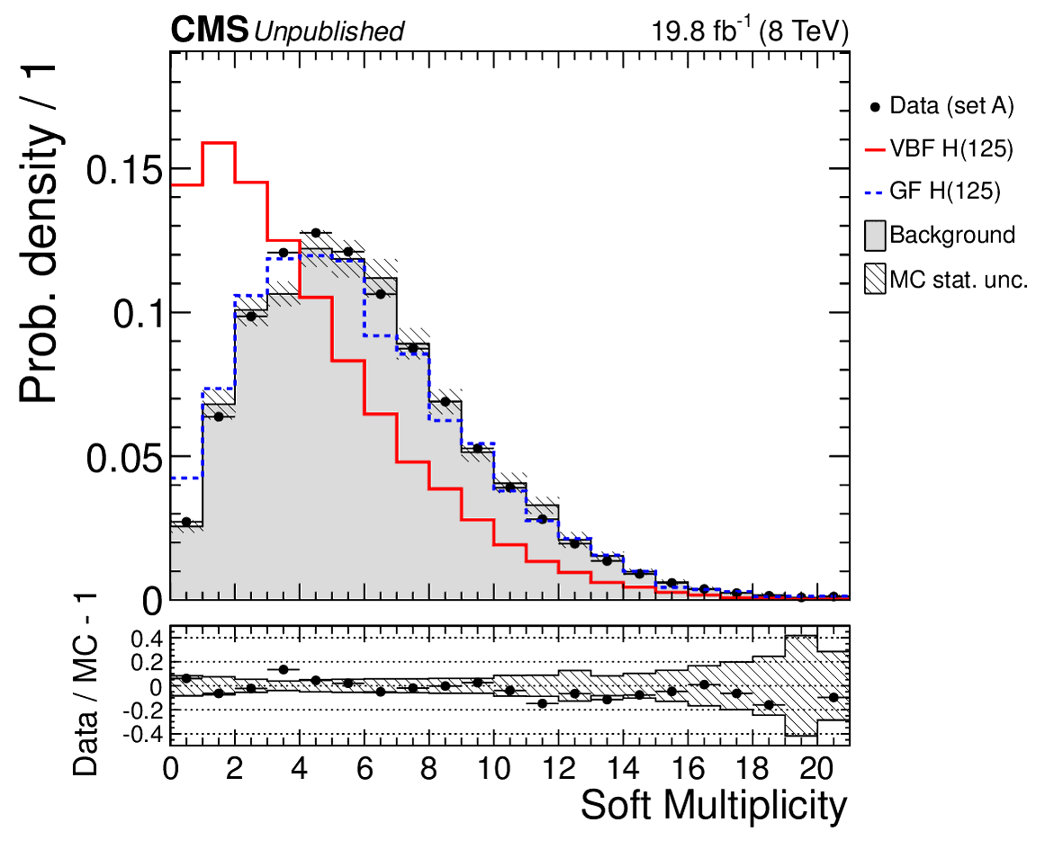
Additional Figure 3:
Normalized distribution of the soft TrackJet multiplicity Nsoft that are associated to the soft QCD activity. The selection corresponds to set A, data is shown with black markers, and background is shown with a filled histogram. The VBF Higgs signal is shown with a solid red line, and the GF Higgs signal is shown with a dashed blue line. The panel at the bottom shows the fractional difference between data and background simulation, with the shaded band representing the MC statistical uncertainty. |

png pdf |
Additional Figure 4:
Normalized distribution of the quark-gluon likelihood discriminant of the second light- jet candidate. Quark jets are expected to have low likelihood values (closer to 0), while gluon jets are expected to have higher ones (closer to 1). The selection corresponds to set A, data is shown with black markers, and background is shown with a filled histogram. The VBF Higgs signal is shown with a solid red line, and the GF Higgs signal is shown with a dashed blue line. The panel at the bottom shows the fractional difference between data and background simulation, with the shaded band representing the MC statistical uncertainty. |

png pdf |
Additional Figure 5:
Simulated invariant mass distribution of the two b-jet candidates before and after the jet pT regression. The generated Higgs-boson mass is 125 GeV and the event selection corresponds to set B. |
png pdf |
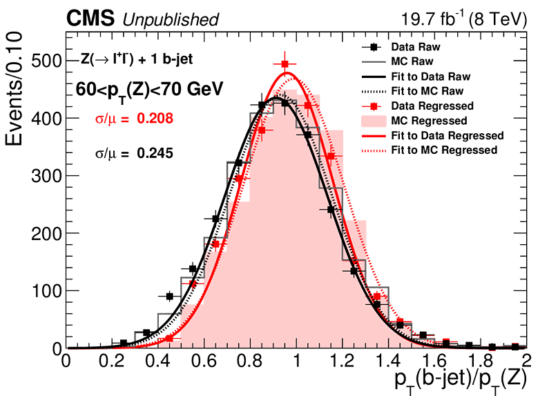
Additional Figure 6:
Ratio of unregressed b-jet pT over Z pT in data and MC for Z(ll)+1 b-jet events in data and simulated events. Events with pT(Z) between 60 and 70 GeV are selected. |
png pdf |
Additional Figure 7-a:
Templates of mbb for $m_{\mathrm{H}} =$ 125GeV in the set A (a) and in the set B (b) selection. The histograms are scaled to the expected number of events. The VBF and GF contributions are weighted with the respective cross sections and stacked. |
png pdf |
Additional Figure 7-b:
Templates of mbb for $m_{\mathrm{H}} =$ 125GeV in the set A (a) and in the set B (b) selection. The histograms are scaled to the expected number of events. The VBF and GF contributions are weighted with the respective cross sections and stacked. |

png pdf |
Additional Figure 8:
Fraction of the GF contribution (GF/(GF + VBF)) per category and per Higgs boson mass. |
png pdf |
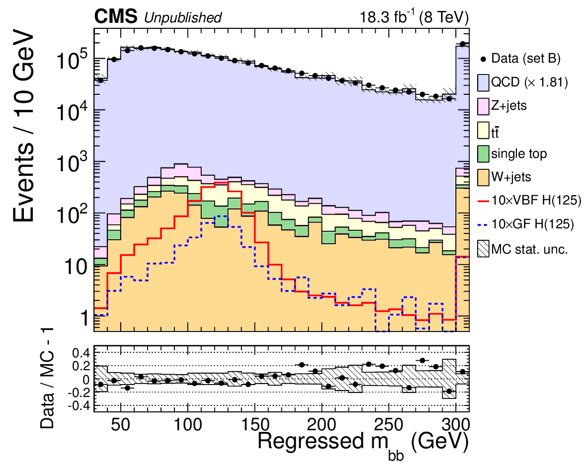
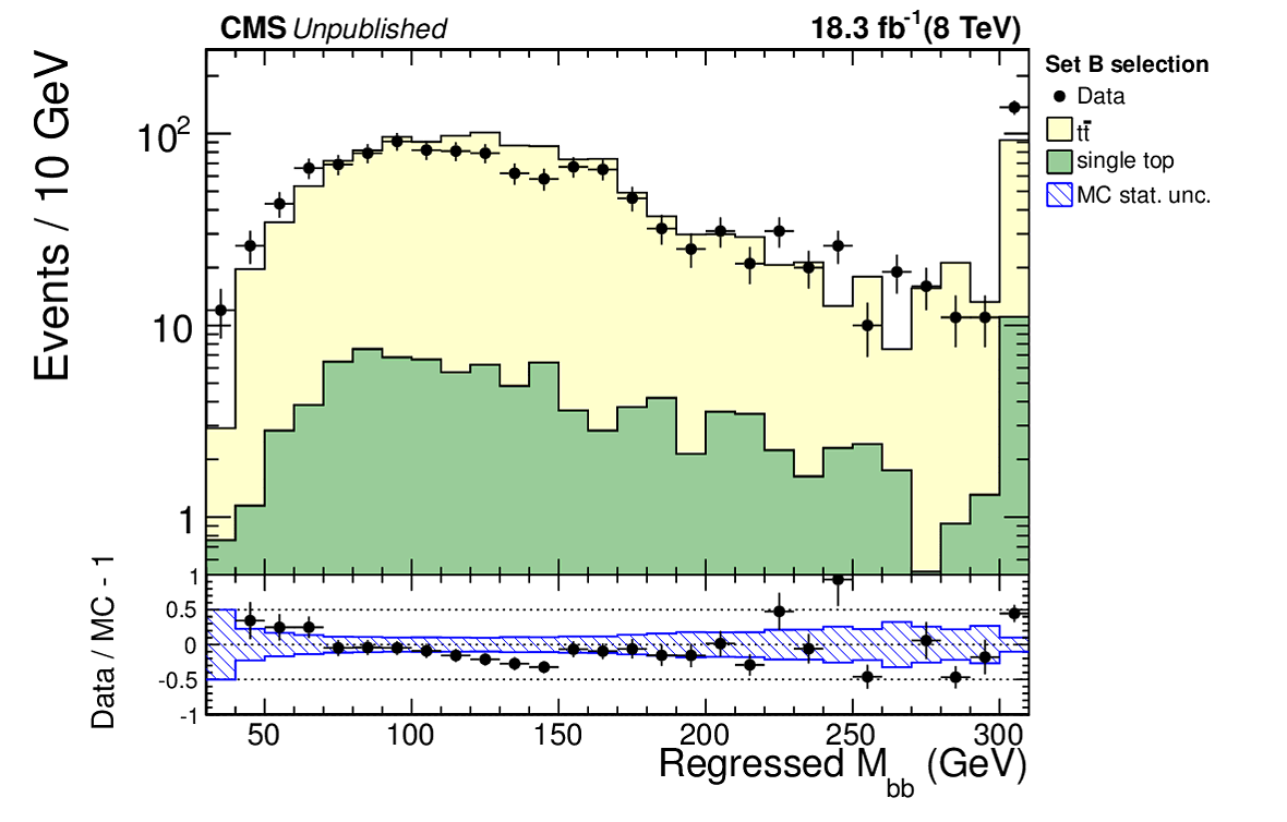
Additional Figure 9:
Distribution of the invariant mass of the two b-jet candidates, after the jet pT regression, for the events of set B. Data is shown with black markers, while the simulated backgrounds are stacked. The LO QCD cross section is multiplied by a factor 1.81 so that the total number of background events equals the number of events in data, while the VBF (red) and GF (blue) Higgs signal yields are amplified by a factor 10. The last bin is the sum of all the events beyond the range of the x axis (overflow). The panels at the bottom show the fractional difference between data and background simulation, with the shaded band representing the MC statistical uncertainty. |
png pdf |
Additional Figure 10-a:
Multivariate discriminants for the Higgs signal in the top control sample for set A (a) and set B (b) selection. Data is shown with black markers, while the simulated backgrounds are stacked. The last bin is the sum of all the events beyond the range of the x axis (overflow). The panels at the bottom show the fractional difference between data and background simulation, with the shaded band representing the MC statistical uncertainty. |
png pdf |
Additional Figure 10-b:
Multivariate discriminants for the Higgs signal in the top control sample for set A (a) and set B (b) selection. Data is shown with black markers, while the simulated backgrounds are stacked. The last bin is the sum of all the events beyond the range of the x axis (overflow). The panels at the bottom show the fractional difference between data and background simulation, with the shaded band representing the MC statistical uncertainty. |
png pdf |
Additional Figure 11-a:
Regressed bb inviariant mass distribution in the top control sample for set A (a) and set B (b) selection. Data is shown with black markers, while the simulated backgrounds are stacked. The last bin is the sum of all the events beyond the range of the x axis (overflow). The panels at the bottom show the fractional difference between data and background simulation, with the shaded band representing the MC statistical uncertainty. |
png pdf |
Additional Figure 11-b:
Regressed bb inviariant mass distribution in the top control sample for set A (a) and set B (b) selection. Data is shown with black markers, while the simulated backgrounds are stacked. The last bin is the sum of all the events beyond the range of the x axis (overflow). The panels at the bottom show the fractional difference between data and background simulation, with the shaded band representing the MC statistical uncertainty. |
png pdf |
Additional Figure 12-a:
Multivariate discriminants for the the Z signal in the top control sample for set A (a) and set B (b) selection. Data is shown with black markers, while the simulated backgrounds are stacked. The last bin is the sum of all the events beyond the range of the x axis (overflow). The panels at the bottom show the fractional difference between data and background simulation, with the shaded band representing the MC statistical uncertainty. |

png pdf |
Additional Figure 12-b:
Multivariate discriminants for the the Z signal in the top control sample for set A (a) and set B (b) selection. Data is shown with black markers, while the simulated backgrounds are stacked. The last bin is the sum of all the events beyond the range of the x axis (overflow). The panels at the bottom show the fractional difference between data and background simulation, with the shaded band representing the MC statistical uncertainty. |
png pdf |
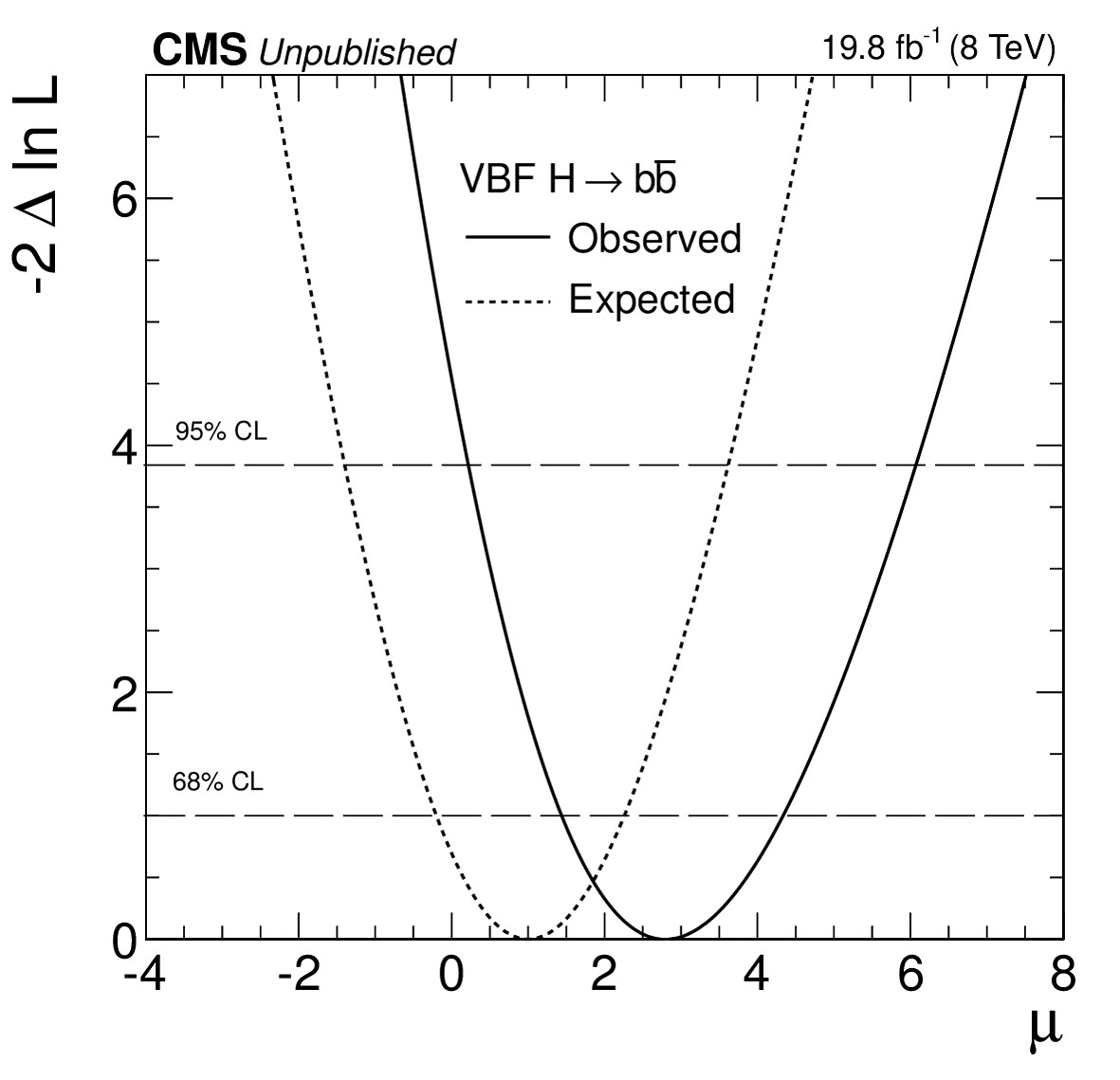
Additional Figure 13:
Observed and SM-expected likelihood profile of the signal strength $\mu = \sigma/\sigma_{SM}$ with $m_{\mathrm{H}} = 125$ GeV. |
png pdf |
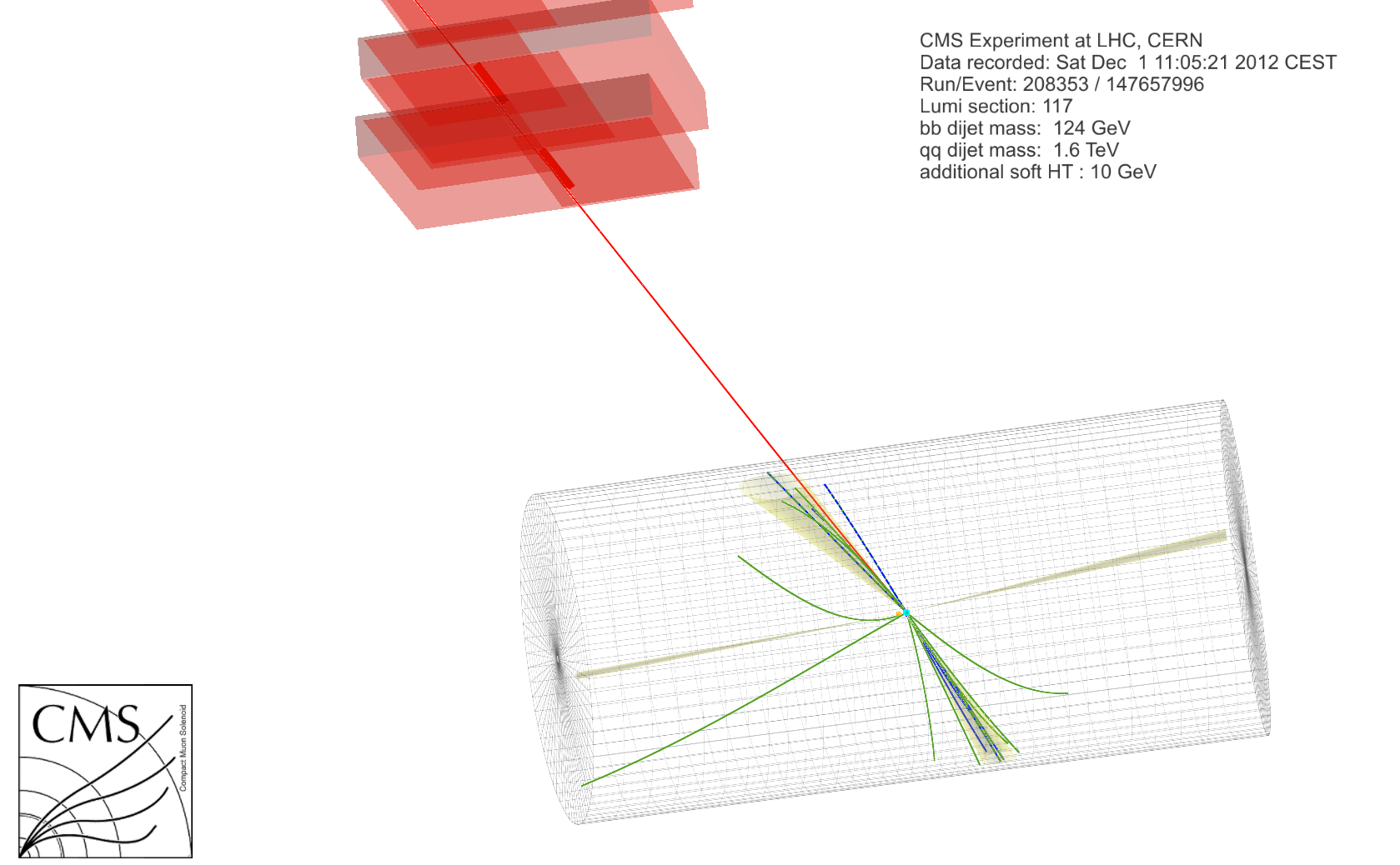
Additional Figure 14-a:
Candidate Signal Event 1. Three dimensional (3D) view (a); Transverse $\rho\phi$ view zoomed near the interaction point (b); Longitudinal $\rho z$ view (c); Combined 3D, $\rho\phi$ and $\rho z$ views (d). |
png pdf |
Additional Figure 14-b:
Candidate Signal Event 1. Three dimensional (3D) view (a); Transverse $\rho\phi$ view zoomed near the interaction point (b); Longitudinal $\rho z$ view (c); Combined 3D, $\rho\phi$ and $\rho z$ views (d). |
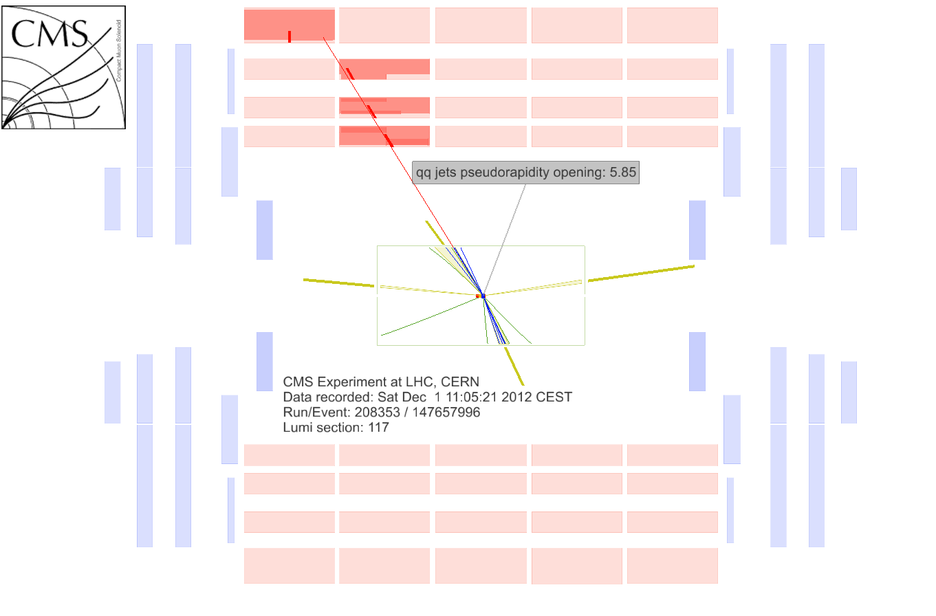
png pdf |
Additional Figure 14-c:
Candidate Signal Event 1. Three dimensional (3D) view (a); Transverse $\rho\phi$ view zoomed near the interaction point (b); Longitudinal $\rho z$ view (c); Combined 3D, $\rho\phi$ and $\rho z$ views (d). |

png pdf |
Additional Figure 14-d:
Candidate Signal Event 1. Three dimensional (3D) view (a); Transverse $\rho\phi$ view zoomed near the interaction point (b); Longitudinal $\rho z$ view (c); Combined 3D, $\rho\phi$ and $\rho z$ views (d). |
png pdf |
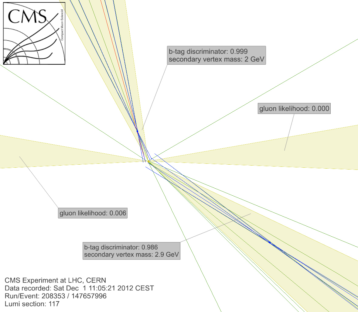
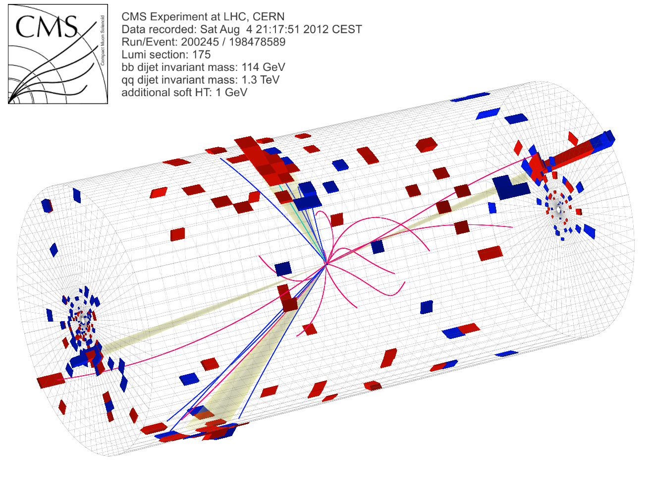
Additional Figure 15-a:
Candidate Signal Event 2. Three dimensional (3D) view (a). The blue tracks are associated to the two central b-jets. The purple tracks contribute to the additional soft HT; |
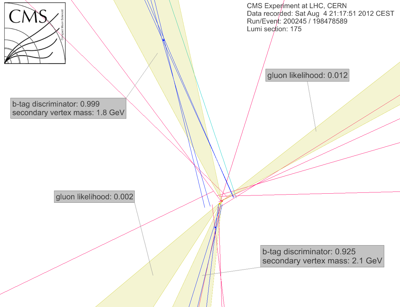
png pdf |
Additional Figure 15-b:
Candidate Signal Event 2. Three dimensional (3D) view (a). The blue tracks are associated to the two central b-jets. The purple tracks contribute to the additional soft HT; |
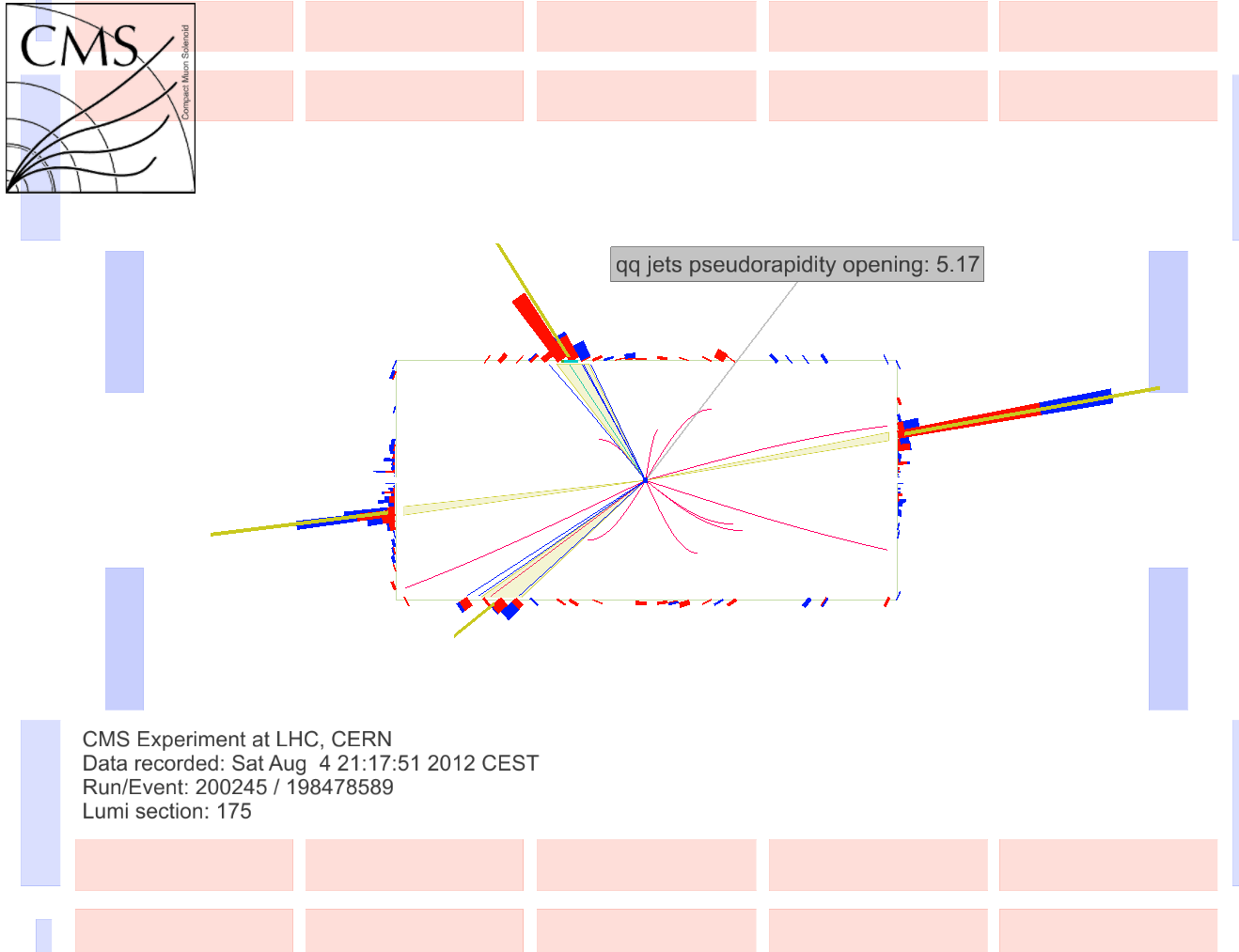
png pdf |
Additional Figure 15-c:
Candidate Signal Event 2. Three dimensional (3D) view (a). The blue tracks are associated to the two central b-jets. The purple tracks contribute to the additional soft HT; |

png pdf |
Additional Figure 15-d:
Candidate Signal Event 2. Three dimensional (3D) view (a). The blue tracks are associated to the two central b-jets. The purple tracks contribute to the additional soft HT; |
png pdf |
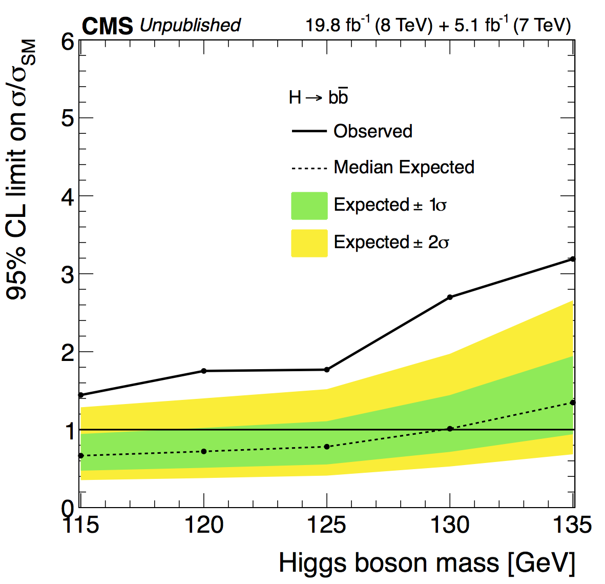
Additional Figure 16:
Expected and observed 95% CL upper limits on the cross section times branching fraction, $\sigma_{\mathrm{H}} \times \mathrm{BR}( \mathrm{ H \rightarrow b\bar{b} } )$, relative to the SM Higgs expectation and as a function of $m_{\mathrm{H}}$, for the combination of the VH, VBF and ttH productions modes and an Higgs boson decaying to bottom quarks. |
png pdf |
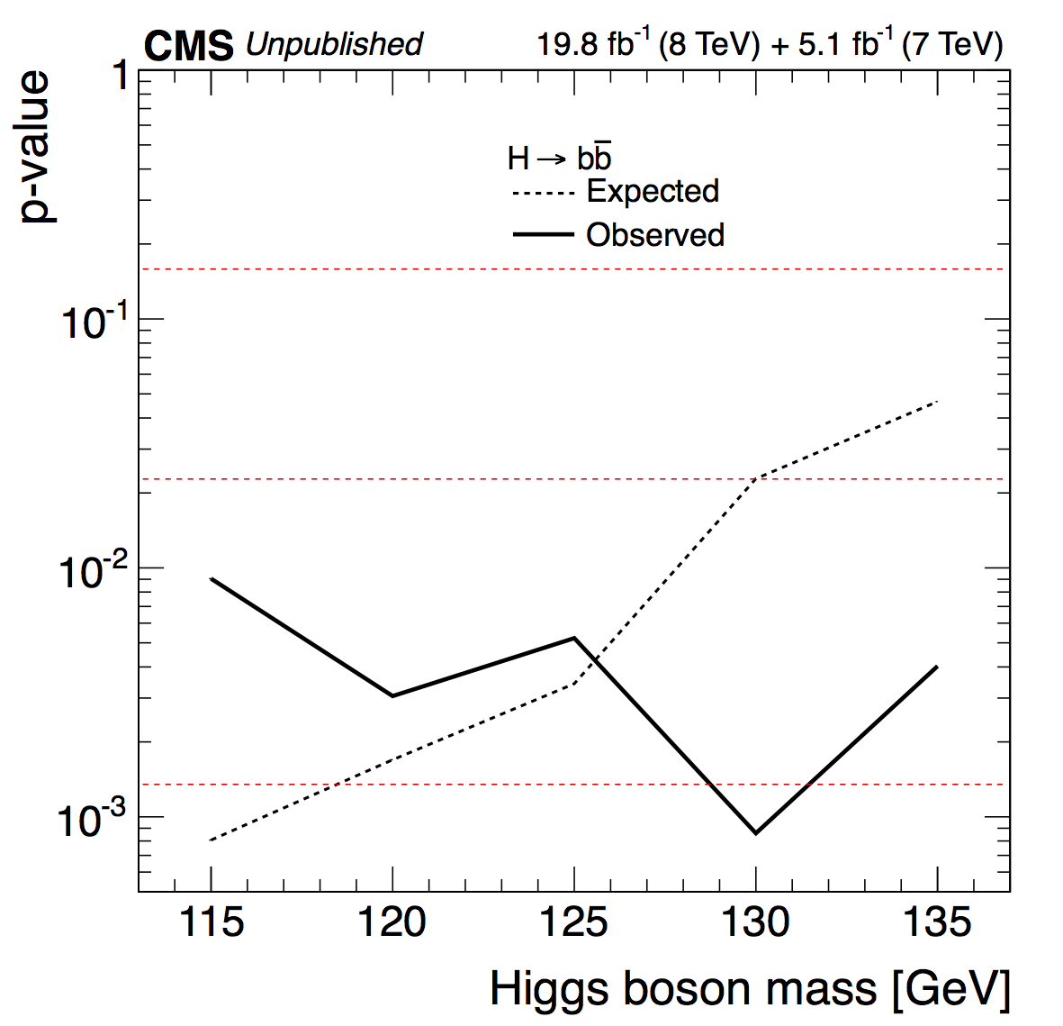
Additional Figure 17:
Expected and observed local p-values for a SM Higgs boson as a function of $m_{\mathrm{H}}$ for the combination of the VH, VBF and ttH productions modes and an Higgs boson decaying to bottom quarks. |
png pdf |
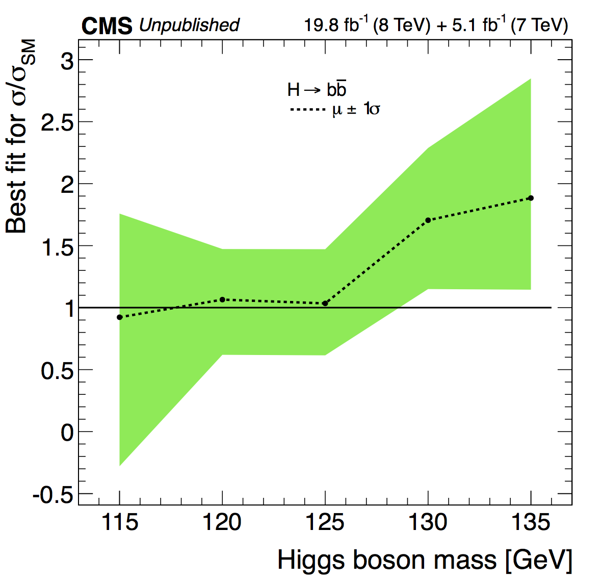
Additional Figure 18:
The observed best-fit signal strength $ \mu_{SM} $ as a function of the SM Higgs boson mass for the combination of the VH, VBF and ttH productions modes and an Higgs boson decaying to bottom quarks. The symbol $\sigma/\sigma_{SM}$ denotes the production cross section times the relevant branching fractions, relative to the SM expectation. The band corresponds to the $\pm 1$ standard deviation uncertainty in $\sigma/\sigma_{SM}$. |
png pdf |
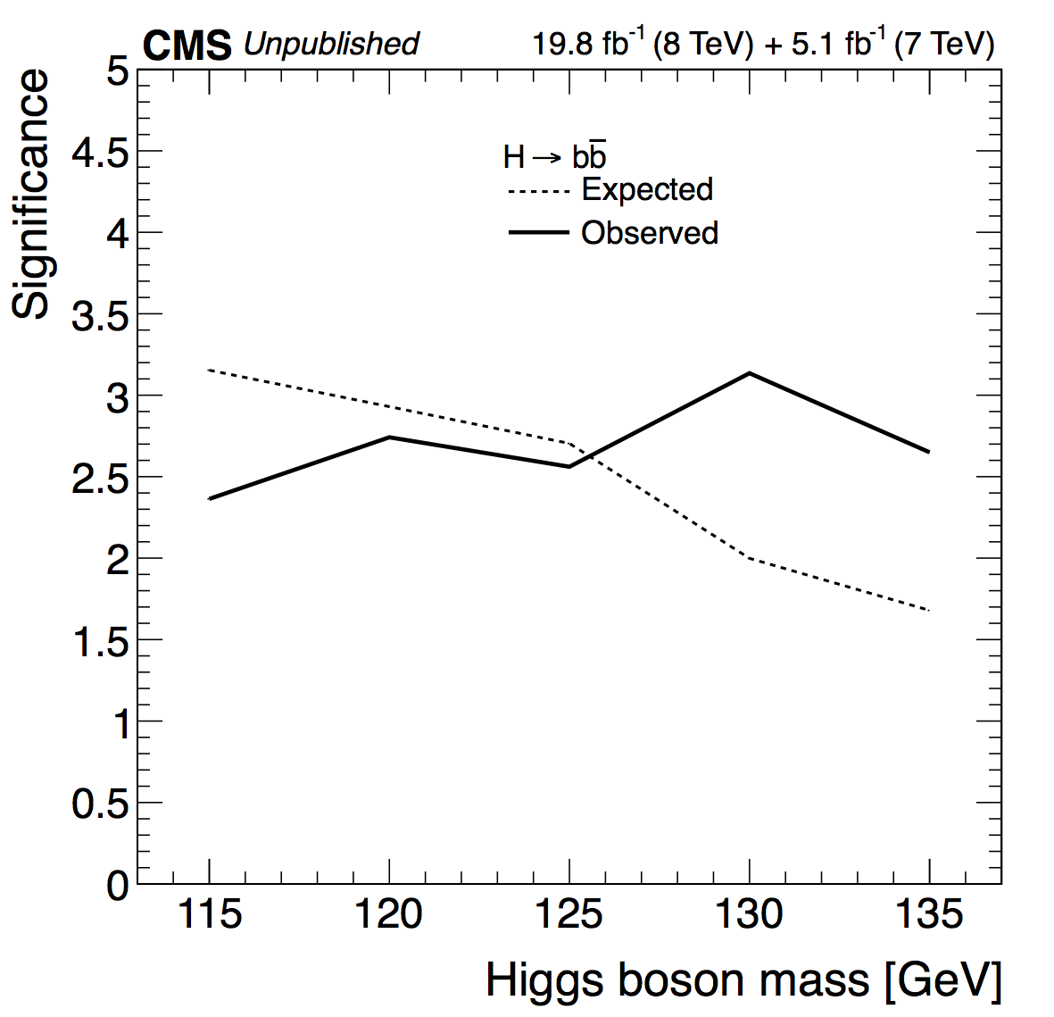
Additional Figure 19:
Expected and observed significances for a SM Higgs boson as a function of $m_{\mathrm{H}}$ for the combination of the VH, VBF and ttH productions modes and an Higgs boson decaying to bottom quarks. |
png pdf |
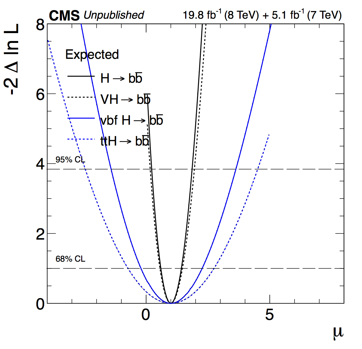
Additional Figure 20:
Likelihood scans of the expected best-fit signal strength $\mu = \sigma/\sigma_{SM}$ for VH, VBF and ttH productions modes and their combination for a Higgs boson decaying to bottom quarks with a mass of 125 GeV. |
png pdf |
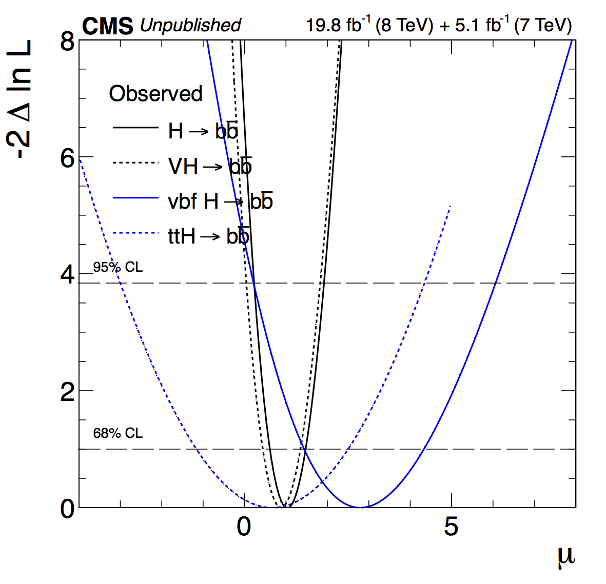
Additional Figure 21:
Likelihood scans of the observed best-fit signal strength $\mu = \sigma/\sigma_{SM}$ for VH, VBF and ttH productions modes and their combination for a Higgs boson decaying to bottom quarks with a mass of 125 GeV. |

png pdf |
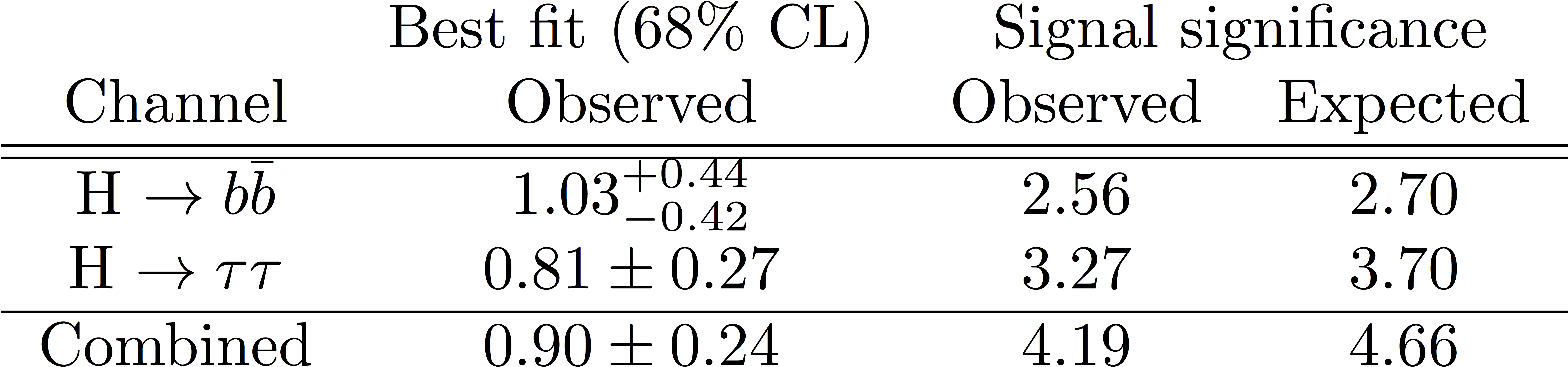
Additional Figure 22:
Likelihood scans of the observed and expected best-fit signal strength $\mu=\sigma/\sigma_{SM}$ for the combination of all $\mathrm{ H\rightarrow b\bar{b} }$ and $\mathrm{ H\rightarrow \tau\tau }$ channels for a Higgs boson with a mass of 125 GeV. |
| Additional Tables | |
png pdf |
Additional Table 1:
Observed and expected on the signal strength parameter $\mu=\sigma/\sigma_{SM}$ and signal significance for $m_{\mathrm{H}}=$125 GeV for the combination of all $\mathrm{ H\rightarrow b\bar{b} }$ and $ \mathrm{ H\rightarrow \tau\tau }$ and their combination. |
|
|
Compact Muon Solenoid LHC, CERN |
|

|

|

|

|

|