

Compact Muon Solenoid
LHC, CERN
| CMS-HIG-14-010 ; CERN-PH-EP-2015-016 | ||
| Search for a standard model Higgs boson produced in association with a top-quark pair and decaying to bottom quarks using a matrix element method | ||
| CMS Collaboration | ||
| 9 February 2015 | ||
| Eur. Phys. J. C 75 (2015) 251 | ||
| Abstract: A search for a standard model Higgs boson produced in association with a top-quark pair and decaying to bottom quarks is presented. Events with hadronic jets and one or two oppositely charged leptons are selected from a data sample corresponding to an integrated luminosity of 19.5 fb$^{-1}$ collected by the CMS experiment at the LHC in pp collisions at a centre-of-mass energy of 8 TeV. In order to separate the signal from the larger $\mathrm{t \bar{t}}$+jets background, this analysis uses a matrix element method that assigns a probability density value to each reconstructed event under signal or background hypotheses. The ratio between the two values is used in a maximum likelihood fit to extract the signal yield. The results are presented in terms of the measured signal strength modifier, $\mu$, relative to the standard model prediction for a Higgs boson mass of 125 GeV. The observed (expected) exclusion limit at a 95% confidence level is $\mu$ lower than 4.2 (3.3), corresponding to a best fit value $\hat{\mu}=1.2^{+1.6}_{-1.5}$. | ||
| Links: e-print arXiv:1502.02485 [hep-ex] (PDF) ; CDS record ; inSPIRE record ; Public twiki page ; HepData record ; CADI line (restricted) ; | ||
| Figures | |
png pdf |
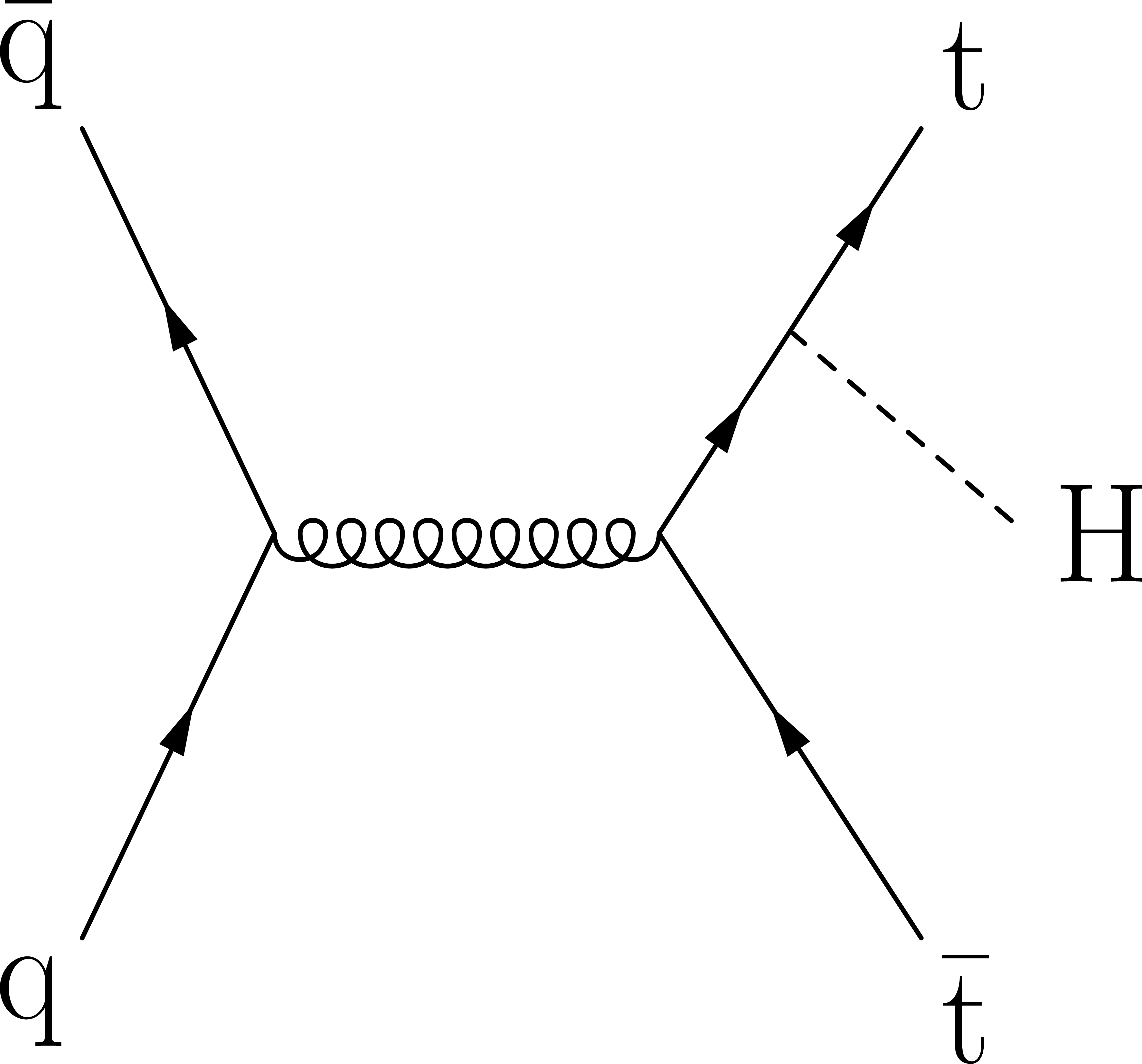
Figure 1-a:
Tree-level Feynman diagrams contributing to the partonic processes: (a) $ { {\mathrm {q}} {\overline {\mathrm {q}}} } \to { {\mathrm {t}\overline {\mathrm {t}}} {\mathrm {H}} }$, (b) $ {\mathrm {g}} {\mathrm {g}} \to { {\mathrm {t}\overline {\mathrm {t}}} {\mathrm {H}} }$, and (c) $ {\mathrm {g}} {\mathrm {g}} \to { {\mathrm {t}\overline {\mathrm {t}}} \mathrm {+} { {\mathrm {b}} {\overline {\mathrm {b}}}} }$. |
png pdf |
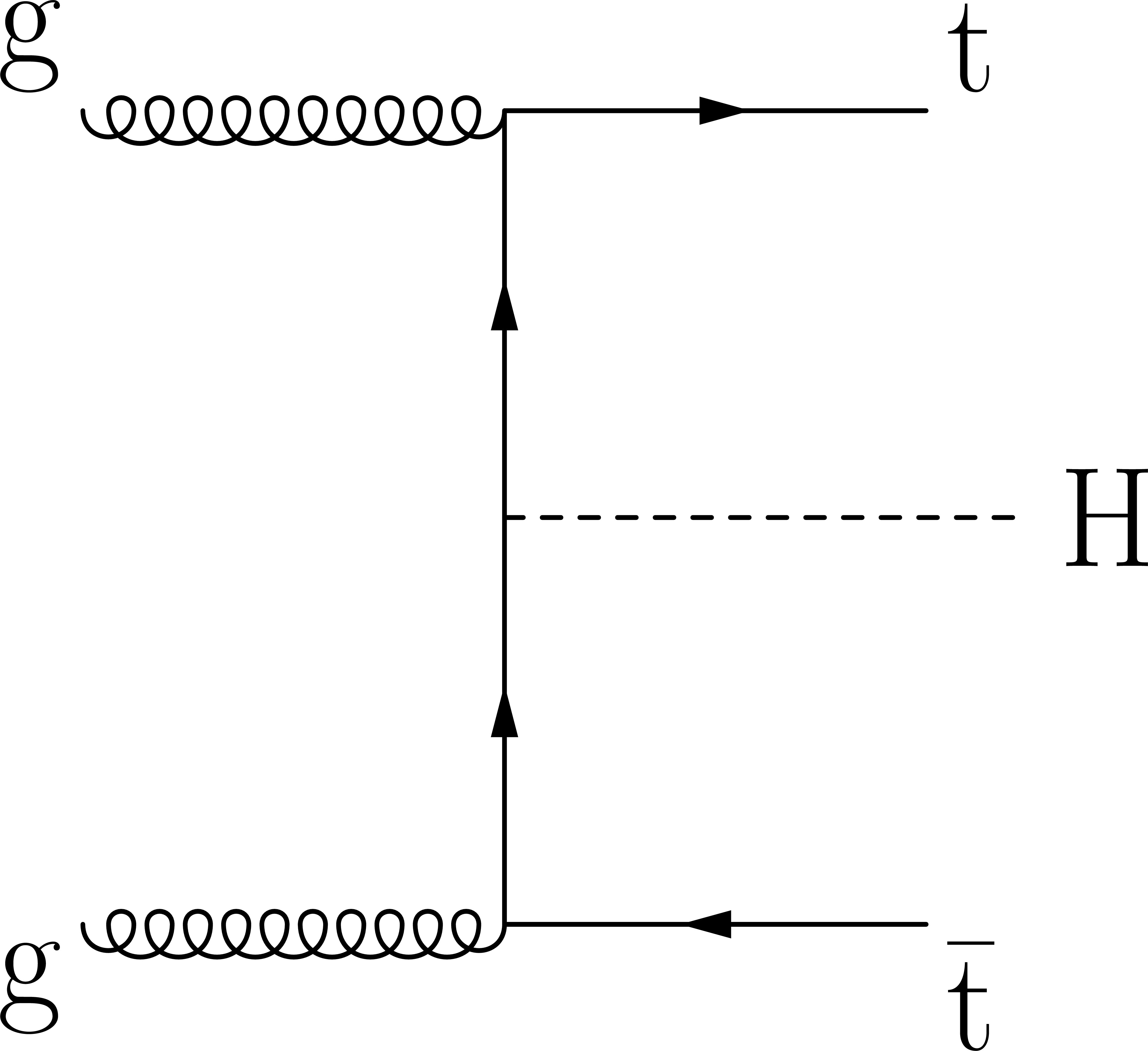
Figure 1-b:
Tree-level Feynman diagrams contributing to the partonic processes: (a) $ { {\mathrm {q}} {\overline {\mathrm {q}}} } \to { {\mathrm {t}\overline {\mathrm {t}}} {\mathrm {H}} }$, (b) $ {\mathrm {g}} {\mathrm {g}} \to { {\mathrm {t}\overline {\mathrm {t}}} {\mathrm {H}} }$, and (c) $ {\mathrm {g}} {\mathrm {g}} \to { {\mathrm {t}\overline {\mathrm {t}}} \mathrm {+} { {\mathrm {b}} {\overline {\mathrm {b}}}} }$. |

png pdf |
Figure 1-c:
Tree-level Feynman diagrams contributing to the partonic processes: (a) $ { {\mathrm {q}} {\overline {\mathrm {q}}} } \to { {\mathrm {t}\overline {\mathrm {t}}} {\mathrm {H}} }$, (b) $ {\mathrm {g}} {\mathrm {g}} \to { {\mathrm {t}\overline {\mathrm {t}}} {\mathrm {H}} }$, and (c) $ {\mathrm {g}} {\mathrm {g}} \to { {\mathrm {t}\overline {\mathrm {t}}} \mathrm {+} { {\mathrm {b}} {\overline {\mathrm {b}}}} }$. |

png pdf |
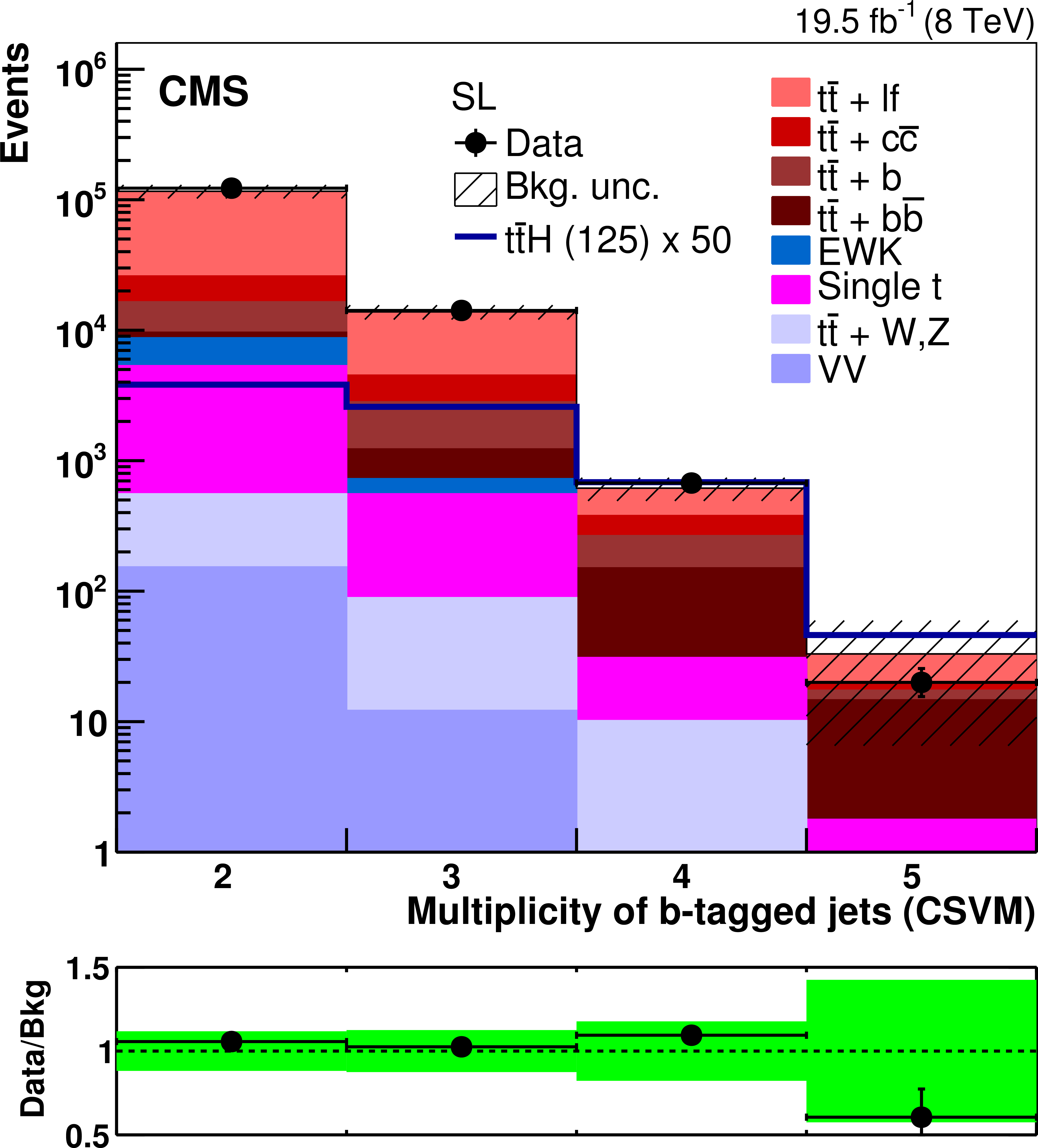
Figure 2-a:
(a,b): distribution of the jet multiplicity in (a) single-lepton and (b) dilepton events, after requiring that at least two jets pass the CSVM working point. c: distribution of the multiplicity of jets passing the CSVM working point in single-lepton events with at least four jets. d: distribution of the selection variable $\mathcal {F}$ defined in Eq. (2) for single-lepton events with at least six jets after requiring a loose preselection of at least one jet passing the CSVM working point. The plots at the bottom of each panel show the ratio between the observed data and the background expectation predicted by the simulation. The shaded and solid green bands corresponds to the total statistical plus systematic uncertainty in the background expectation described in Section 7. More details on the background modelling are provided in Section 6.3. |

png pdf |
Figure 2-b:
(a,b): distribution of the jet multiplicity in (a) single-lepton and (b) dilepton events, after requiring that at least two jets pass the CSVM working point. c: distribution of the multiplicity of jets passing the CSVM working point in single-lepton events with at least four jets. d: distribution of the selection variable $\mathcal {F}$ defined in Eq. (2) for single-lepton events with at least six jets after requiring a loose preselection of at least one jet passing the CSVM working point. The plots at the bottom of each panel show the ratio between the observed data and the background expectation predicted by the simulation. The shaded and solid green bands corresponds to the total statistical plus systematic uncertainty in the background expectation described in Section 7. More details on the background modelling are provided in Section 6.3. |
png pdf |
Figure 2-c:
(a,b): distribution of the jet multiplicity in (a) single-lepton and (b) dilepton events, after requiring that at least two jets pass the CSVM working point. c: distribution of the multiplicity of jets passing the CSVM working point in single-lepton events with at least four jets. d: distribution of the selection variable $\mathcal {F}$ defined in Eq. (2) for single-lepton events with at least six jets after requiring a loose preselection of at least one jet passing the CSVM working point. The plots at the bottom of each panel show the ratio between the observed data and the background expectation predicted by the simulation. The shaded and solid green bands corresponds to the total statistical plus systematic uncertainty in the background expectation described in Section 7. More details on the background modelling are provided in Section 6.3. |
png pdf |
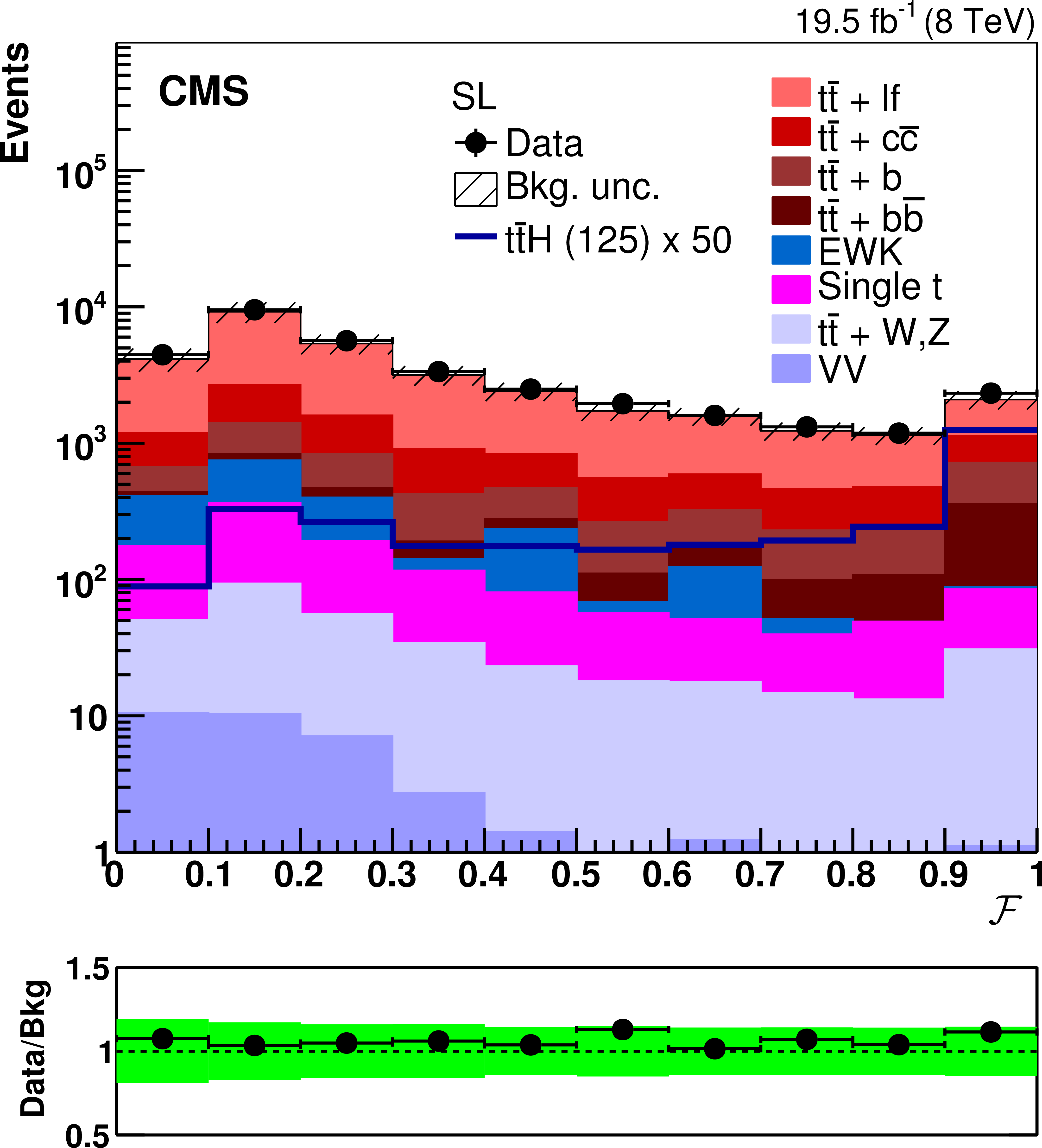
Figure 2-d:
(a,b): distribution of the jet multiplicity in (a) single-lepton and (b) dilepton events, after requiring that at least two jets pass the CSVM working point. c: distribution of the multiplicity of jets passing the CSVM working point in single-lepton events with at least four jets. d: distribution of the selection variable $\mathcal {F}$ defined in Eq. (2) for single-lepton events with at least six jets after requiring a loose preselection of at least one jet passing the CSVM working point. The plots at the bottom of each panel show the ratio between the observed data and the background expectation predicted by the simulation. The shaded and solid green bands corresponds to the total statistical plus systematic uncertainty in the background expectation described in Section 7. More details on the background modelling are provided in Section 6.3. |
png pdf |
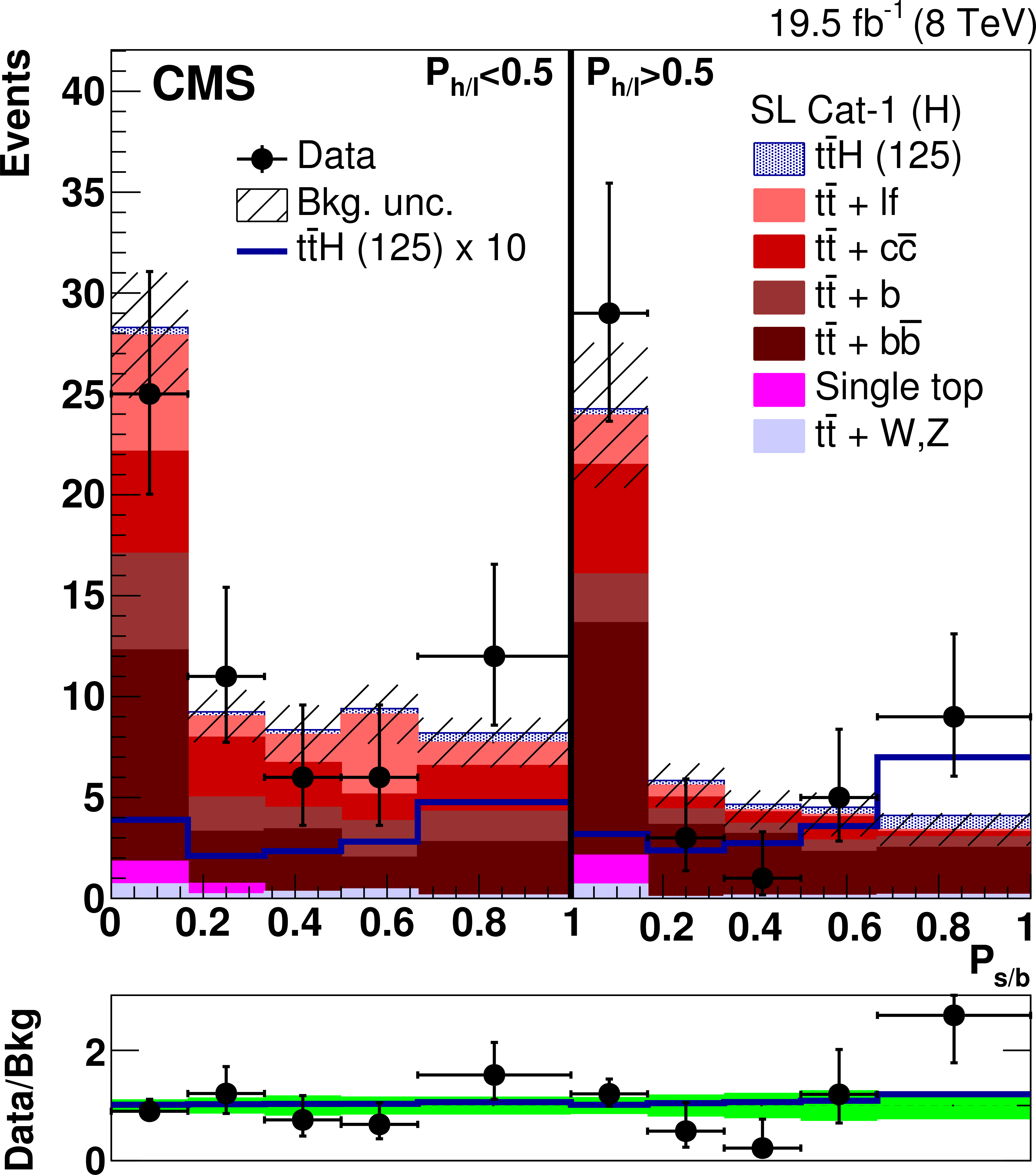
Figure 3-a:
Distribution of the $P_{\mathrm {s/b}}$ discriminant in the two $P_{\mathrm {h/l}}$ bins for the high-purity (H) categories. The signal and background yields have been obtained from a combined fit of all nuisance parameters with the constraint $\mu =1$. The bottom panel of each plot shows the ratio between the observed and the overall background yields. The solid blue line indicates the ratio between the signal-plus-background and the background-only distributions. The shaded and solid green bands band correspond to the $\pm 1\sigma $ uncertainty in the background prediction after the fit. |

png pdf |
Figure 3-b:
Distribution of the $P_{\mathrm {s/b}}$ discriminant in the two $P_{\mathrm {h/l}}$ bins for the high-purity (H) categories. The signal and background yields have been obtained from a combined fit of all nuisance parameters with the constraint $\mu =1$. The bottom panel of each plot shows the ratio between the observed and the overall background yields. The solid blue line indicates the ratio between the signal-plus-background and the background-only distributions. The shaded and solid green bands band correspond to the $\pm 1\sigma $ uncertainty in the background prediction after the fit. |
png pdf |
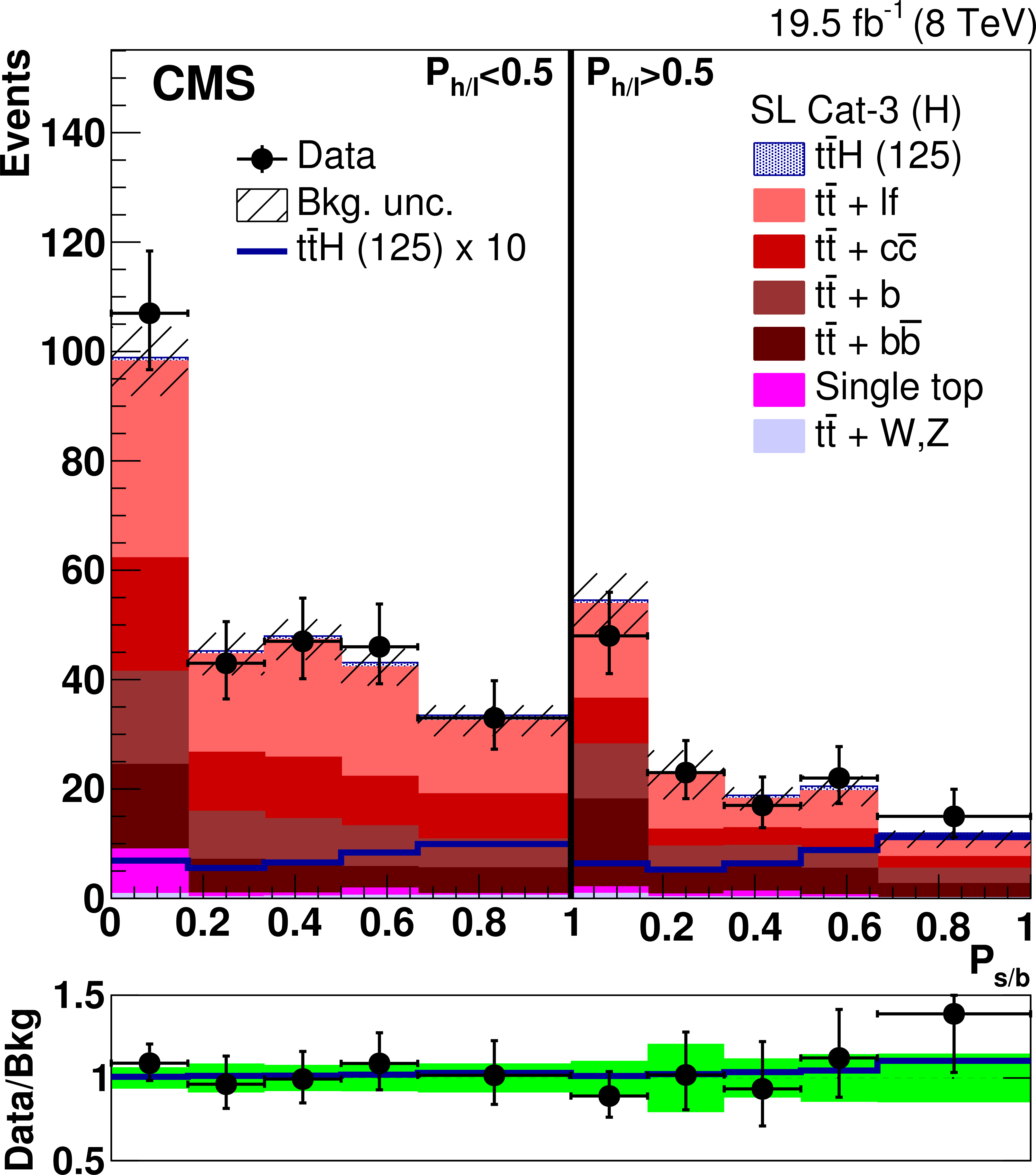
Figure 3-c:
Distribution of the $P_{\mathrm {s/b}}$ discriminant in the two $P_{\mathrm {h/l}}$ bins for the high-purity (H) categories. The signal and background yields have been obtained from a combined fit of all nuisance parameters with the constraint $\mu =1$. The bottom panel of each plot shows the ratio between the observed and the overall background yields. The solid blue line indicates the ratio between the signal-plus-background and the background-only distributions. The shaded and solid green bands band correspond to the $\pm 1\sigma $ uncertainty in the background prediction after the fit. |

png pdf |
Figure 3-d:
Distribution of the $P_{\mathrm {s/b}}$ discriminant in the two $P_{\mathrm {h/l}}$ bins for the high-purity (H) categories. The signal and background yields have been obtained from a combined fit of all nuisance parameters with the constraint $\mu =1$. The bottom panel of each plot shows the ratio between the observed and the overall background yields. The solid blue line indicates the ratio between the signal-plus-background and the background-only distributions. The shaded and solid green bands band correspond to the $\pm 1\sigma $ uncertainty in the background prediction after the fit. |
png pdf |
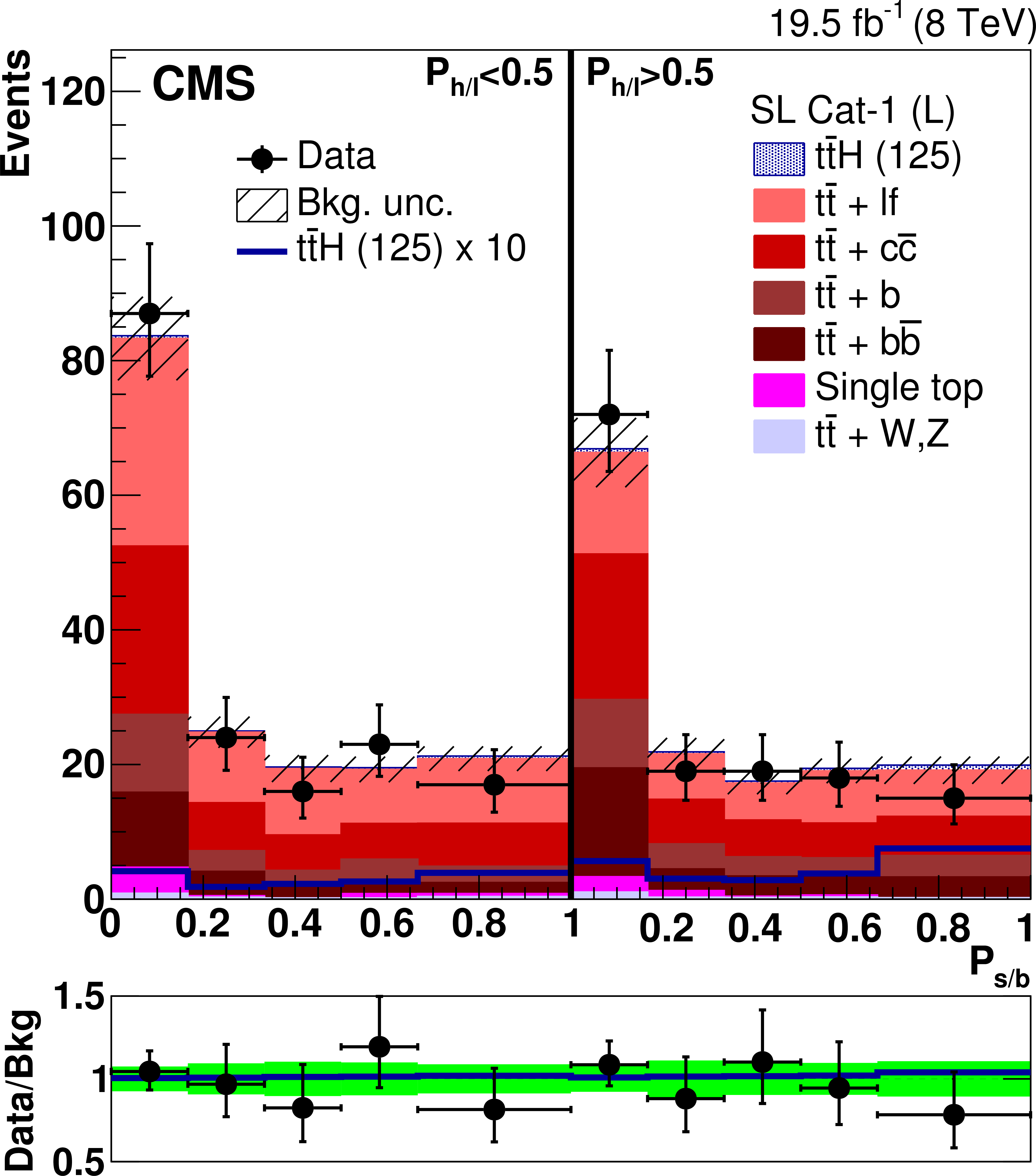
Figure 4-a:
Distribution of the $P_{\mathrm {s/b}}$ discriminant in the two $P_{\mathrm {h/l}}$ bins for the low-purity (L) categories. The signal and background yields have been obtained from a combined fit of all nuisance parameters with the constraint $\mu =1$. The bottom panel of each plot shows the ratio between the observed and the overall background yields. The solid blue line indicates the ratio between the signal-plus-background and the background-only distributions. The shaded and solid green bands correspond to the $\pm 1\sigma $ uncertainty in the background prediction after the fit. |

png pdf |
Figure 4-b:
Distribution of the $P_{\mathrm {s/b}}$ discriminant in the two $P_{\mathrm {h/l}}$ bins for the low-purity (L) categories. The signal and background yields have been obtained from a combined fit of all nuisance parameters with the constraint $\mu =1$. The bottom panel of each plot shows the ratio between the observed and the overall background yields. The solid blue line indicates the ratio between the signal-plus-background and the background-only distributions. The shaded and solid green bands correspond to the $\pm 1\sigma $ uncertainty in the background prediction after the fit. |

png pdf |
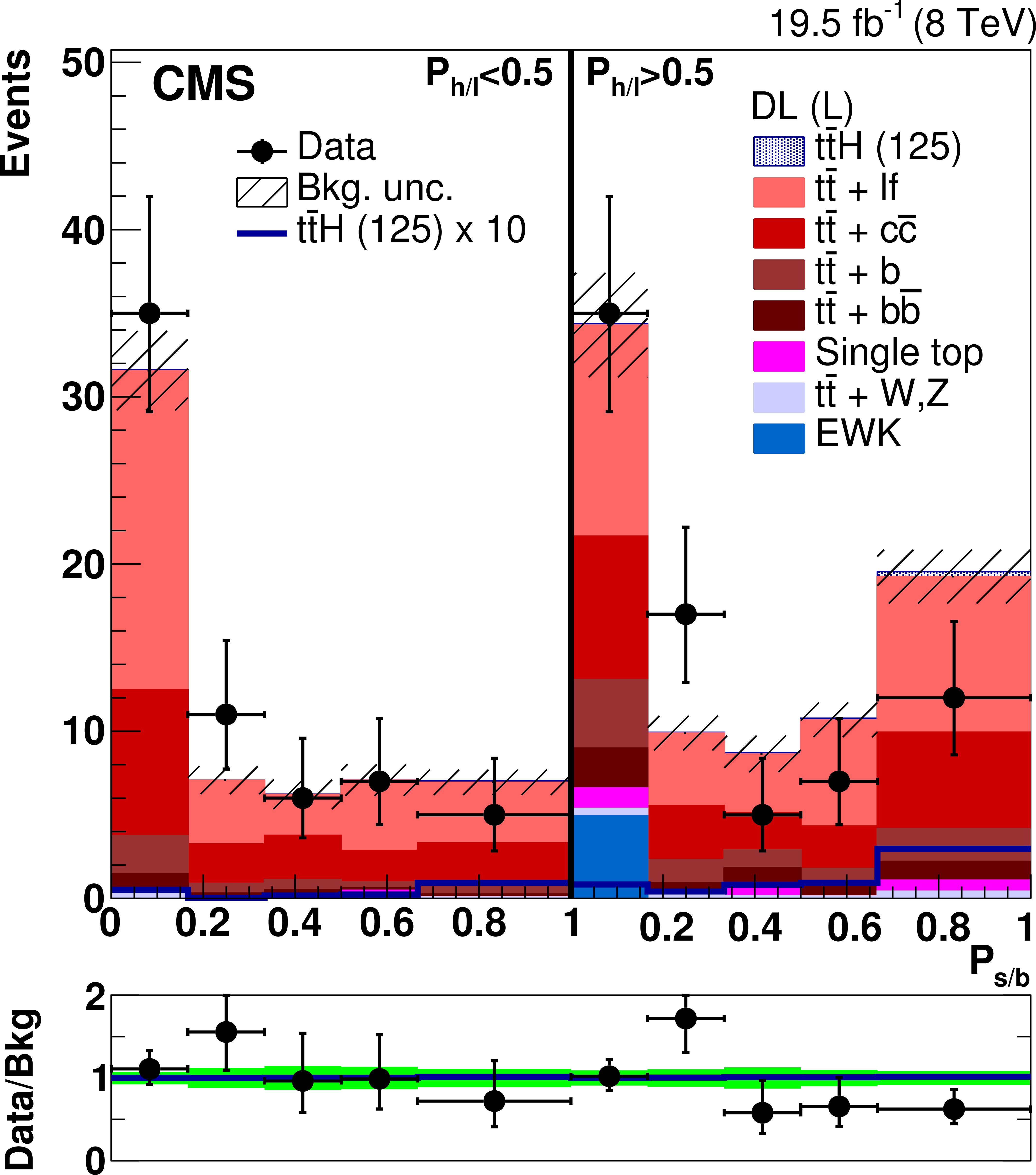
Figure 4-c:
Distribution of the $P_{\mathrm {s/b}}$ discriminant in the two $P_{\mathrm {h/l}}$ bins for the low-purity (L) categories. The signal and background yields have been obtained from a combined fit of all nuisance parameters with the constraint $\mu =1$. The bottom panel of each plot shows the ratio between the observed and the overall background yields. The solid blue line indicates the ratio between the signal-plus-background and the background-only distributions. The shaded and solid green bands correspond to the $\pm 1\sigma $ uncertainty in the background prediction after the fit. |
png pdf |
Figure 4-d:
Distribution of the $P_{\mathrm {s/b}}$ discriminant in the two $P_{\mathrm {h/l}}$ bins for the low-purity (L) categories. The signal and background yields have been obtained from a combined fit of all nuisance parameters with the constraint $\mu =1$. The bottom panel of each plot shows the ratio between the observed and the overall background yields. The solid blue line indicates the ratio between the signal-plus-background and the background-only distributions. The shaded and solid green bands correspond to the $\pm 1\sigma $ uncertainty in the background prediction after the fit. |

png pdf |
Figure 5-a:
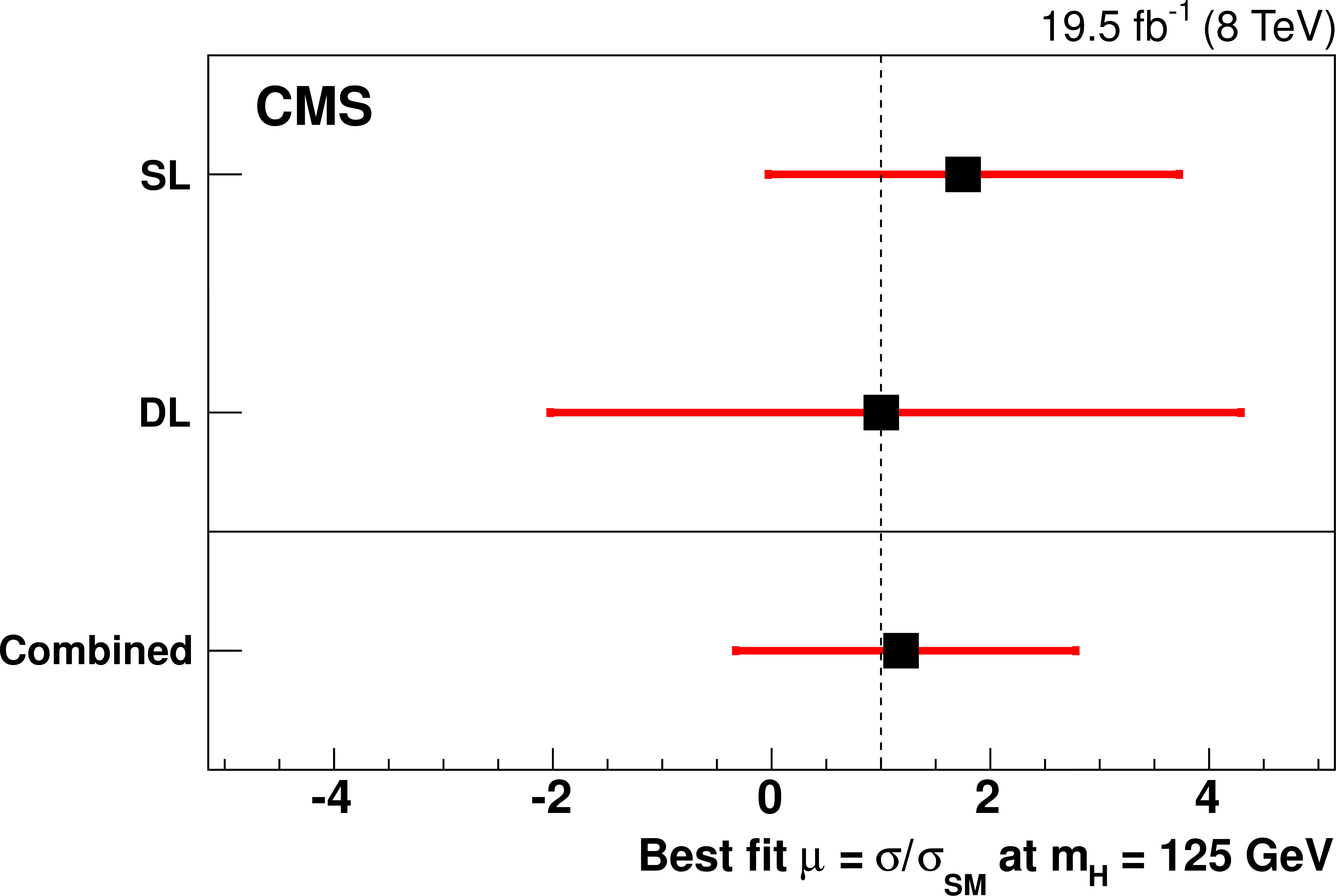
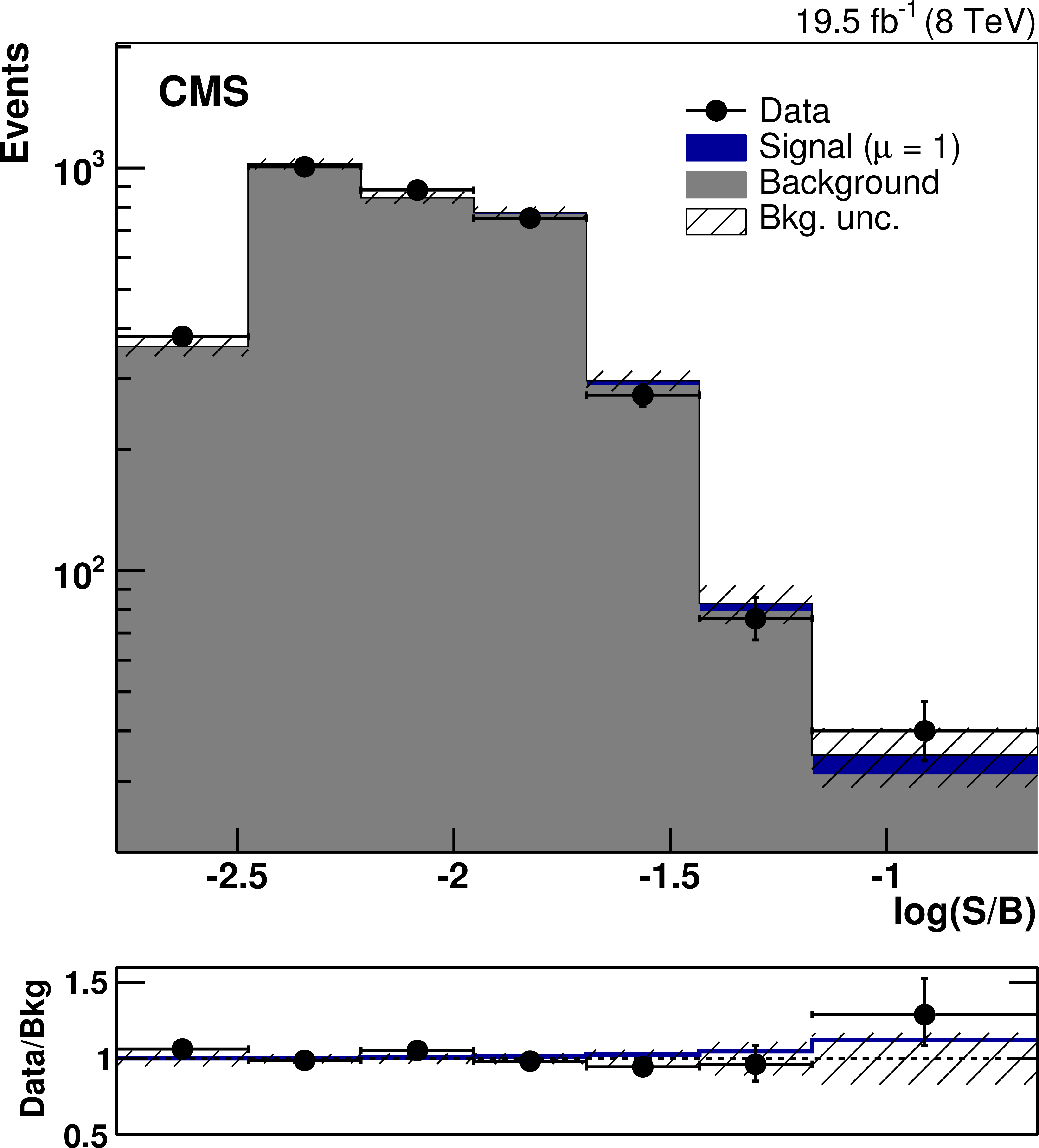
(top left) Observed 95% CL UL on $\mu $ are compared to the median expected limits under the background-only and the signal-plus-background hypotheses. The former are shown together with their ${\pm }1\sigma $ and ${\pm }2\sigma $ CL intervals. Results are shown separately for the individual channels and for their combination. (top right) Best-fit value of the signal strength modifier $\mu $ with its $\pm 1\sigma $ CL interval obtained from the individual channels and from their combination. (bottom) Distribution of the decimal logarithm $\log(\mathrm {S}/\mathrm {B})$, where $\mathrm {S}$ ($\mathrm {B}$) indicates the total signal (background) yield expected in the bins of the two-dimensional histograms, as obtained from a combined fit with the constraint $\mu =1$. |
png pdf |
Figure 5-b:
(top left) Observed 95% CL UL on $\mu $ are compared to the median expected limits under the background-only and the signal-plus-background hypotheses. The former are shown together with their ${\pm }1\sigma $ and ${\pm }2\sigma $ CL intervals. Results are shown separately for the individual channels and for their combination. (top right) Best-fit value of the signal strength modifier $\mu $ with its $\pm 1\sigma $ CL interval obtained from the individual channels and from their combination. (bottom) Distribution of the decimal logarithm $\log(\mathrm {S}/\mathrm {B})$, where $\mathrm {S}$ ($\mathrm {B}$) indicates the total signal (background) yield expected in the bins of the two-dimensional histograms, as obtained from a combined fit with the constraint $\mu =1$. |
png pdf |
Figure 5-c:
(top left) Observed 95% CL UL on $\mu $ are compared to the median expected limits under the background-only and the signal-plus-background hypotheses. The former are shown together with their ${\pm }1\sigma $ and ${\pm }2\sigma $ CL intervals. Results are shown separately for the individual channels and for their combination. (top right) Best-fit value of the signal strength modifier $\mu $ with its $\pm 1\sigma $ CL interval obtained from the individual channels and from their combination. (bottom) Distribution of the decimal logarithm $\log(\mathrm {S}/\mathrm {B})$, where $\mathrm {S}$ ($\mathrm {B}$) indicates the total signal (background) yield expected in the bins of the two-dimensional histograms, as obtained from a combined fit with the constraint $\mu =1$. |
|
|
Compact Muon Solenoid LHC, CERN |
|

|

|

|

|

|