

Compact Muon Solenoid
LHC, CERN
| CMS-HIG-14-011 ; CERN-PH-EP-2015-088 | ||
| Search for a pseudoscalar boson decaying into a Z boson and the 125 GeV Higgs boson in $\mathrm{\ell^+ \ell^- b \bar{b}}$ final states | ||
| CMS Collaboration | ||
| 19 April 2015 | ||
| Phys. Lett. B 748 (2015) 221 | ||
| Abstract: Results are reported on a search for decays of a pseudoscalar A boson into a Z boson and a light scalar h boson, where the Z boson decays into a pair of oppositely-charged electrons or muons, and the h boson decays into $\mathrm{b \bar{b}}$. The search is based on data from proton-proton collisions at a center-of-mass energy $\sqrt{s}$ = 8 TeV collected with the CMS detector, corresponding to an integrated luminosity of 19.7 fb$^{-1}$. The h boson is assumed to be the recently discovered standard model-like Higgs boson with a mass of 125 GeV. With no evidence for signal, upper limits are obtained on the product of the production cross section and the branching fraction of the A boson in the Zh channel. Results are also interpreted in the context of two Higgs doublet models. | ||
| Links: e-print arXiv:1504.04710 [hep-ex] (PDF) ; CDS record ; inSPIRE record ; Public twiki page ; HepData record ; CADI line (restricted) ; | ||
| Figures | Summary | Additional Figures | CMS Publications |
|---|
| Figures | |
png pdf |
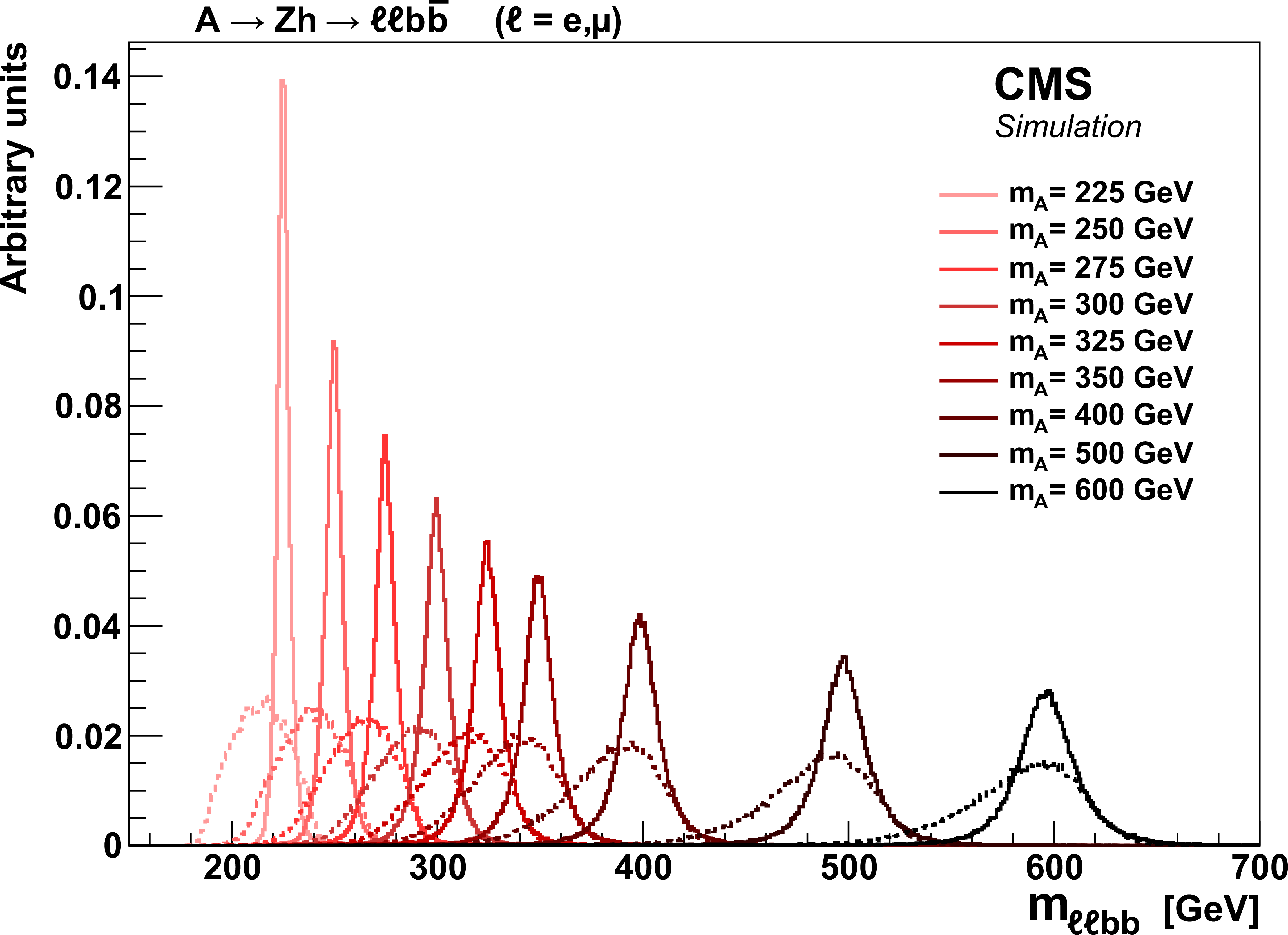
Figure 1:
Simulated distributions for $ m_{\ell \ell {\mathrm {bb}} }$ before (dotted lines) and after the kinematic fits (solid lines). Histograms are normalized to unit area. |
png pdf |
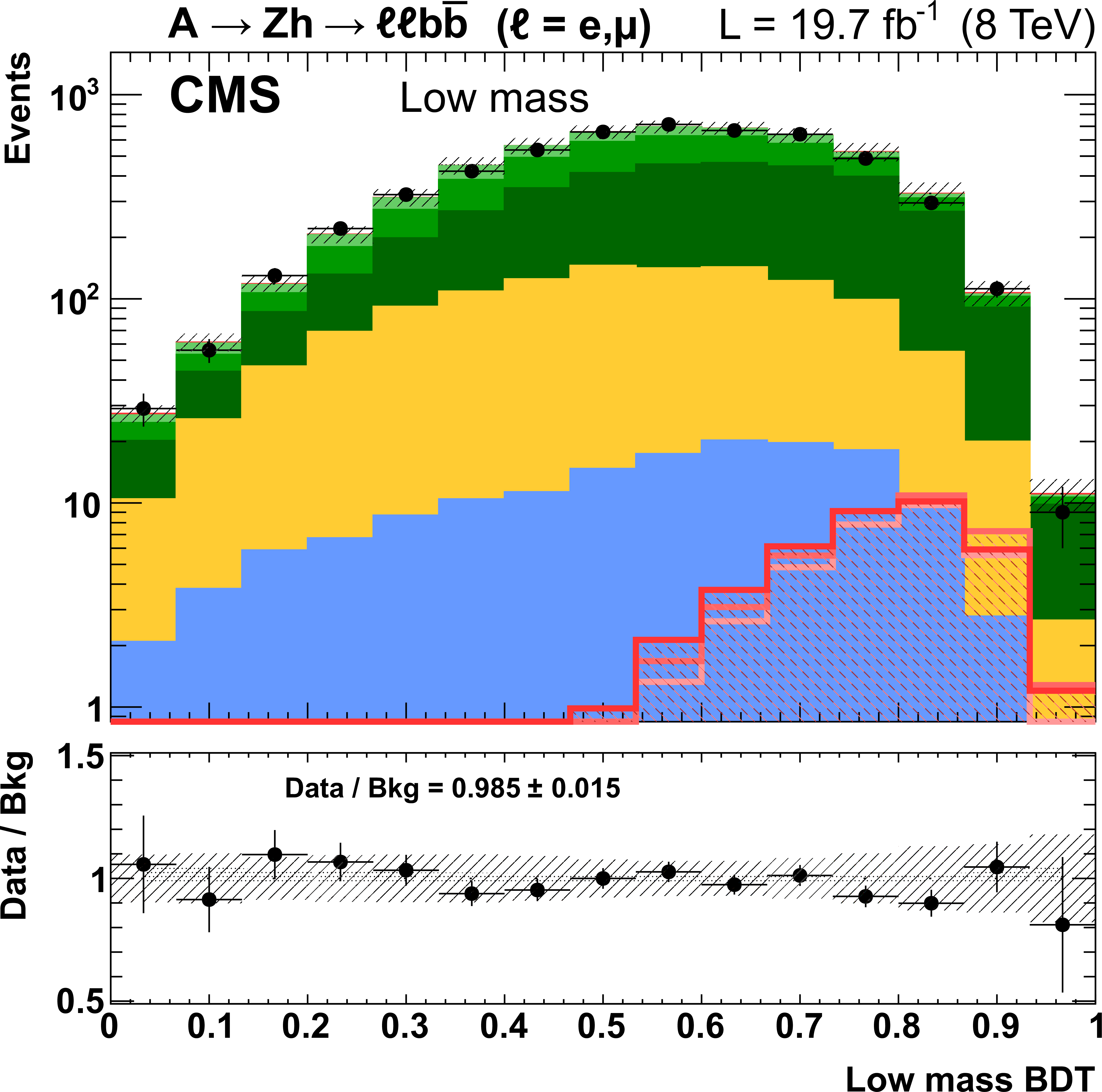
Figure 2-a:
BDT outputs (a, c, e) and invariant mass distributions (b, d, f) in the low (a, b), intermediate (c, d), and high (e, f) mass regions. The $ m_{\ell \ell {\mathrm {bb}} }$ plots are for $\mathrm {BDT}>0.6$, weighted by $\mathrm {S/(S+B)}$ in each BDT bin. Histograms for signal are normalized to the expected exclusion limit at 95% confidence level. Statistical and systematic uncertainties in simulated samples are shown as well. Either the ratio (a, c, e) or the difference (b, d, f) between data and SM background is given at the bottom of each panel. |
png pdf |
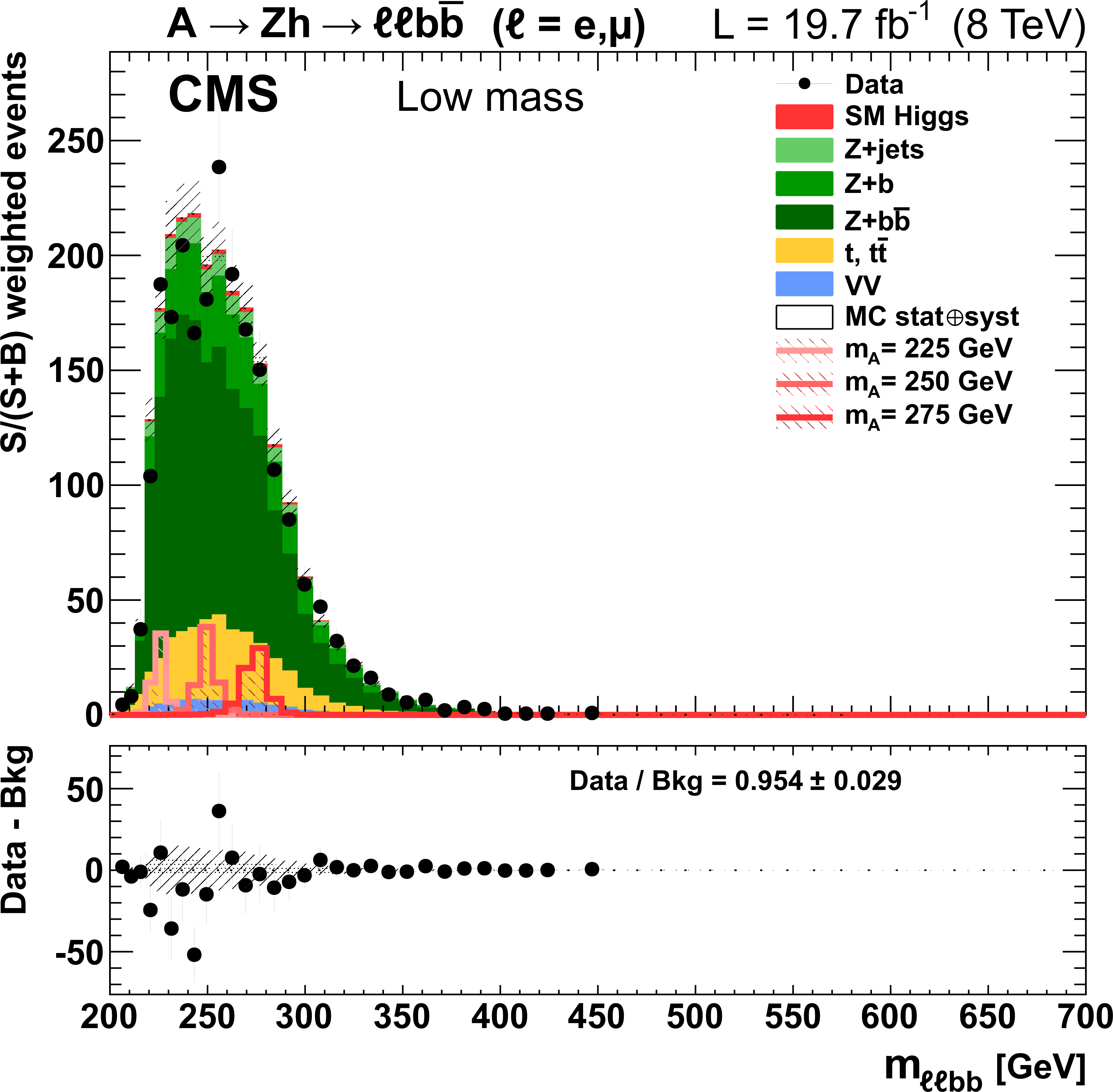
Figure 2-b:
BDT outputs (a, c, e) and invariant mass distributions (b, d, f) in the low (a, b), intermediate (c, d), and high (e, f) mass regions. The $ m_{\ell \ell {\mathrm {bb}} }$ plots are for $\mathrm {BDT}>0.6$, weighted by $\mathrm {S/(S+B)}$ in each BDT bin. Histograms for signal are normalized to the expected exclusion limit at 95% confidence level. Statistical and systematic uncertainties in simulated samples are shown as well. Either the ratio (a, c, e) or the difference (b, d, f) between data and SM background is given at the bottom of each panel. |

png pdf |
Figure 2-c:
BDT outputs (a, c, e) and invariant mass distributions (b, d, f) in the low (a, b), intermediate (c, d), and high (e, f) mass regions. The $ m_{\ell \ell {\mathrm {bb}} }$ plots are for $\mathrm {BDT}>0.6$, weighted by $\mathrm {S/(S+B)}$ in each BDT bin. Histograms for signal are normalized to the expected exclusion limit at 95% confidence level. Statistical and systematic uncertainties in simulated samples are shown as well. Either the ratio (a, c, e) or the difference (b, d, f) between data and SM background is given at the bottom of each panel. |

png pdf |
Figure 2-d:
BDT outputs (a, c, e) and invariant mass distributions (b, d, f) in the low (a, b), intermediate (c, d), and high (e, f) mass regions. The $ m_{\ell \ell {\mathrm {bb}} }$ plots are for $\mathrm {BDT}>0.6$, weighted by $\mathrm {S/(S+B)}$ in each BDT bin. Histograms for signal are normalized to the expected exclusion limit at 95% confidence level. Statistical and systematic uncertainties in simulated samples are shown as well. Either the ratio (a, c, e) or the difference (b, d, f) between data and SM background is given at the bottom of each panel. |
png pdf |
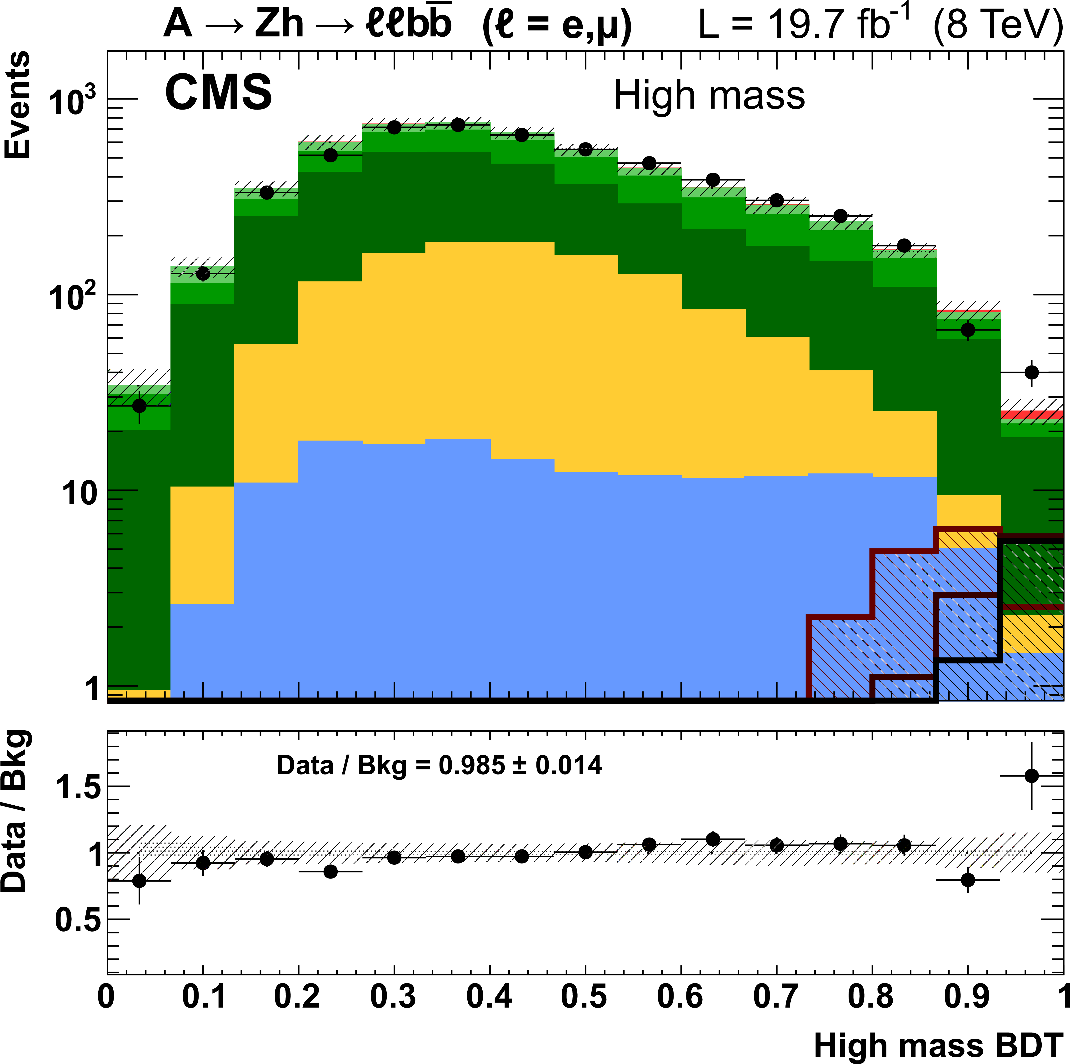
Figure 2-e:
BDT outputs (a, c, e) and invariant mass distributions (b, d, f) in the low (a, b), intermediate (c, d), and high (e, f) mass regions. The $ m_{\ell \ell {\mathrm {bb}} }$ plots are for $\mathrm {BDT}>0.6$, weighted by $\mathrm {S/(S+B)}$ in each BDT bin. Histograms for signal are normalized to the expected exclusion limit at 95% confidence level. Statistical and systematic uncertainties in simulated samples are shown as well. Either the ratio (a, c, e) or the difference (b, d, f) between data and SM background is given at the bottom of each panel. |

png pdf |
Figure 2-f:
BDT outputs (a, c, e) and invariant mass distributions (b, d, f) in the low (a, b), intermediate (c, d), and high (e, f) mass regions. The $ m_{\ell \ell {\mathrm {bb}} }$ plots are for $\mathrm {BDT}>0.6$, weighted by $\mathrm {S/(S+B)}$ in each BDT bin. Histograms for signal are normalized to the expected exclusion limit at 95% confidence level. Statistical and systematic uncertainties in simulated samples are shown as well. Either the ratio (a, c, e) or the difference (b, d, f) between data and SM background is given at the bottom of each panel. |
png pdf |
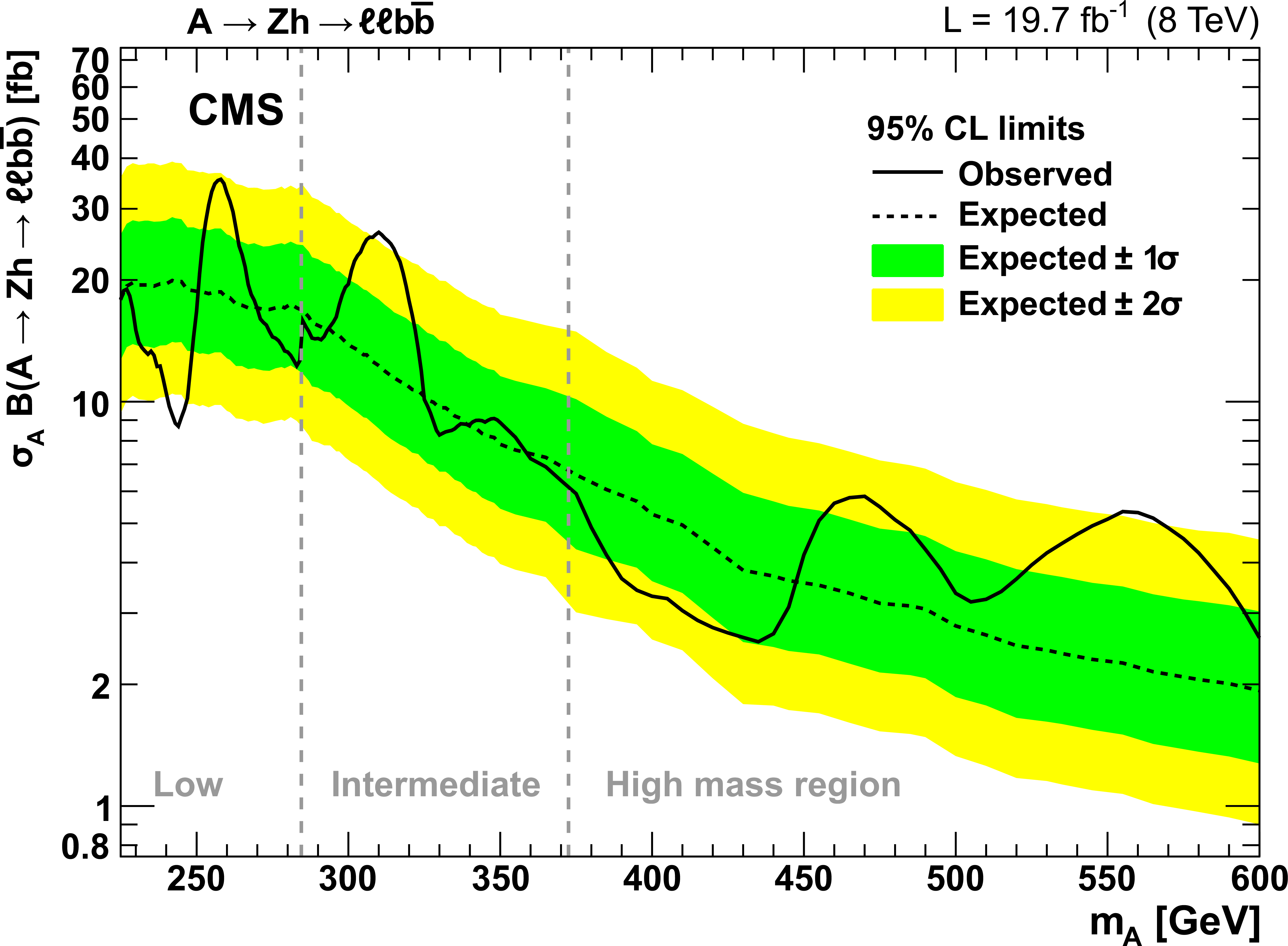
Figure 3:
Observed and expected 95% CL upper limit on $\sigma _ {\mathrm {A}} {\mathcal {B}}({\mathrm {A}} \to {\mathrm {Z}} {\mathrm {h}} \to {\ell \ell }{\mathrm {b \bar{b} } } )$ as a function of $m_{{\mathrm {A}}}$ in the narrow-width approximation, including all statistical and systematic uncertainties. The green and yellow bands are the ${\pm }1$ and ${\pm }2\sigma $ uncertainty bands on the expected limit. |

png pdf |
Figure 4-a:
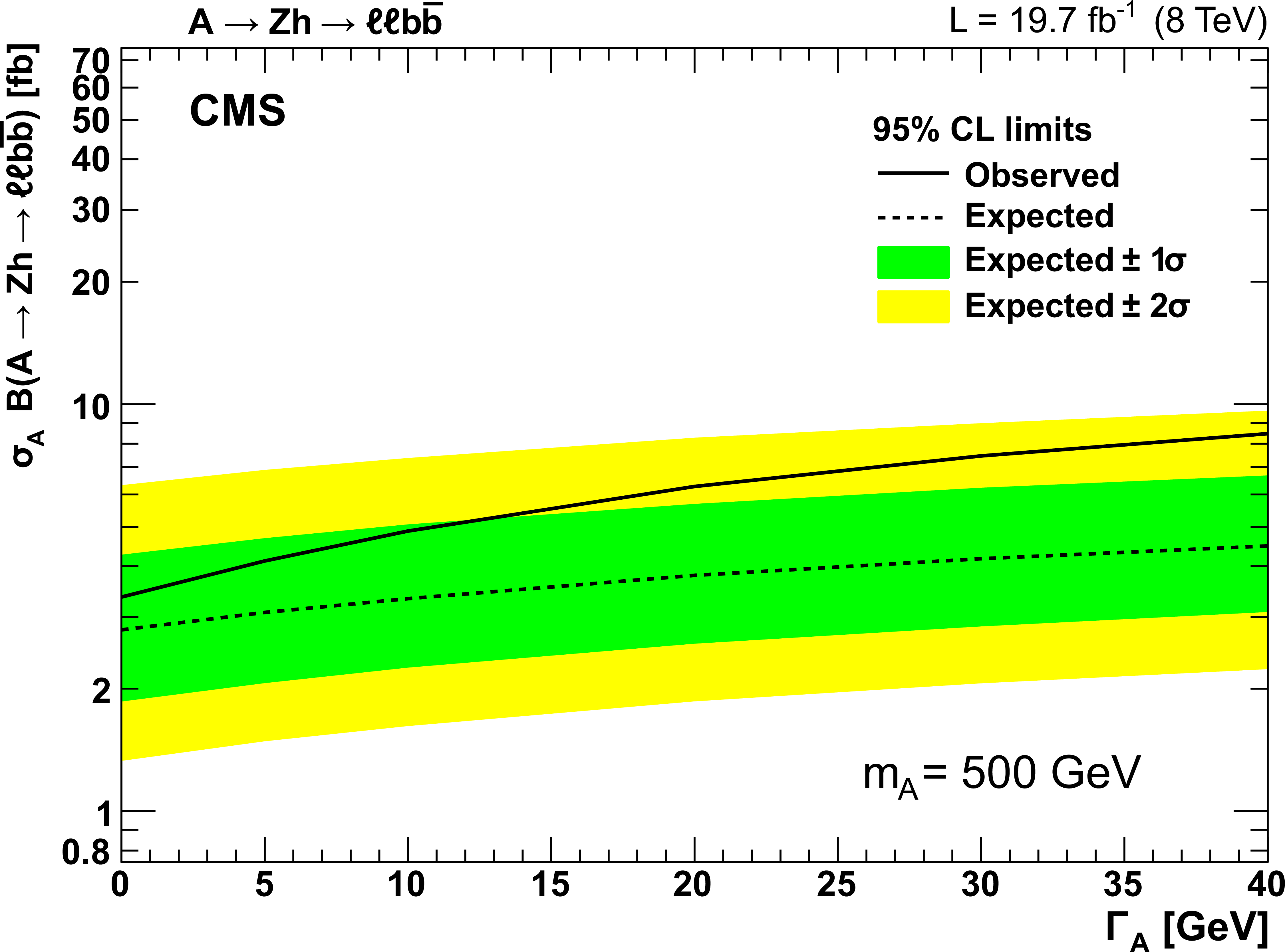
Observed and expected 95% CL upper limit on $\sigma _ {\mathrm {A}} {\mathcal {B}}({\mathrm {A}} \to {\mathrm {Z}} {\mathrm {h}} \to {\ell \ell }{\mathrm {b \bar{b} } } )\, $ for $\Gamma _{\mathrm {A}} =30$ GeV as a function of $m_ {\mathrm {A}}$ (a), and for $m_ {\mathrm {A}} = 500$ GeV as a function of the width of the A boson (b). |
png pdf |
Figure 4-b:
Observed and expected 95% CL upper limit on $\sigma _ {\mathrm {A}} {\mathcal {B}}({\mathrm {A}} \to {\mathrm {Z}} {\mathrm {h}} \to {\ell \ell }{\mathrm {b \bar{b} } } )\, $ for $\Gamma _{\mathrm {A}} =30$ GeV as a function of $m_ {\mathrm {A}}$ (a), and for $m_ {\mathrm {A}} = 500$ GeV as a function of the width of the A boson (b). |
png pdf |
Figure 5-a:
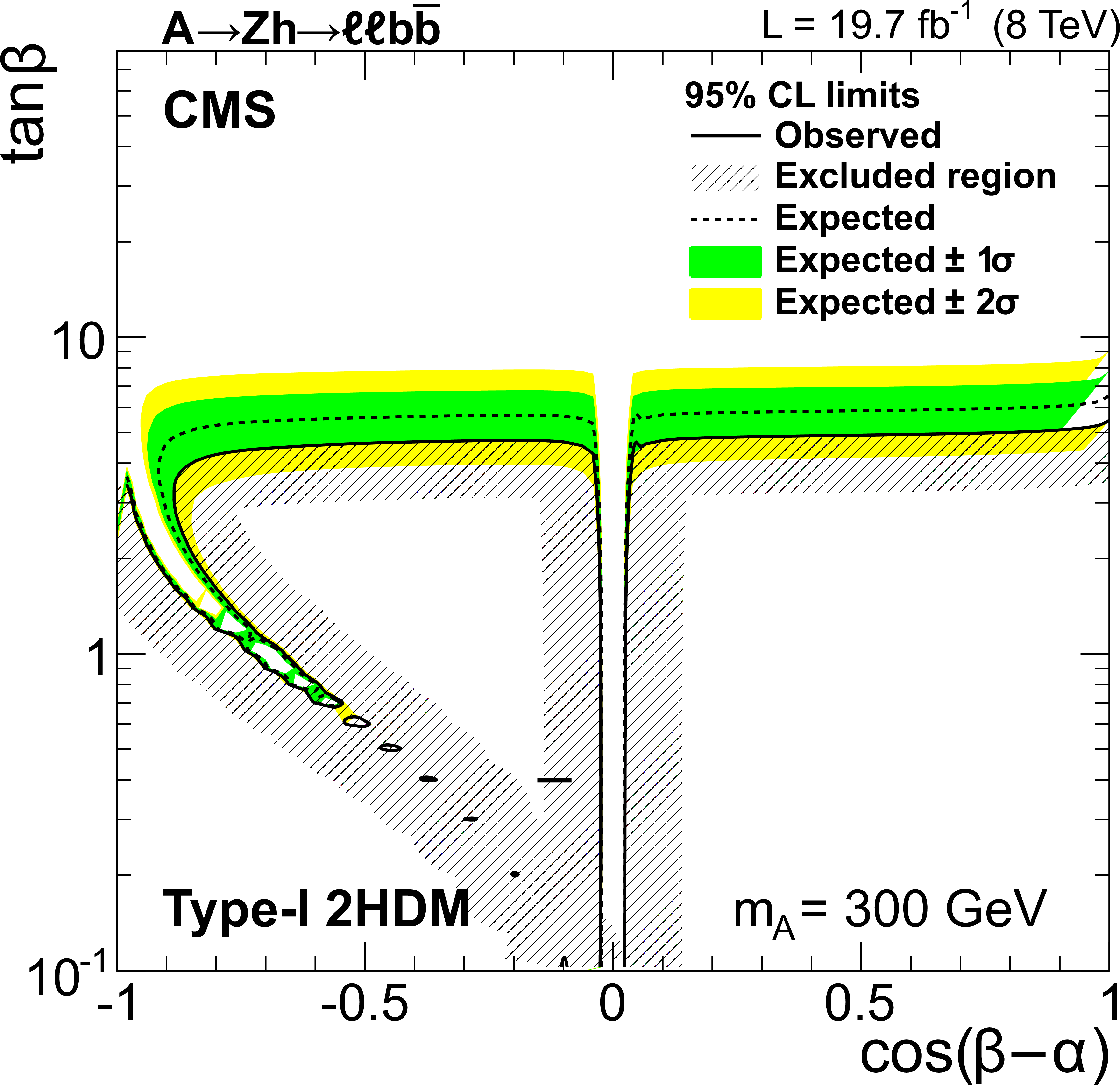
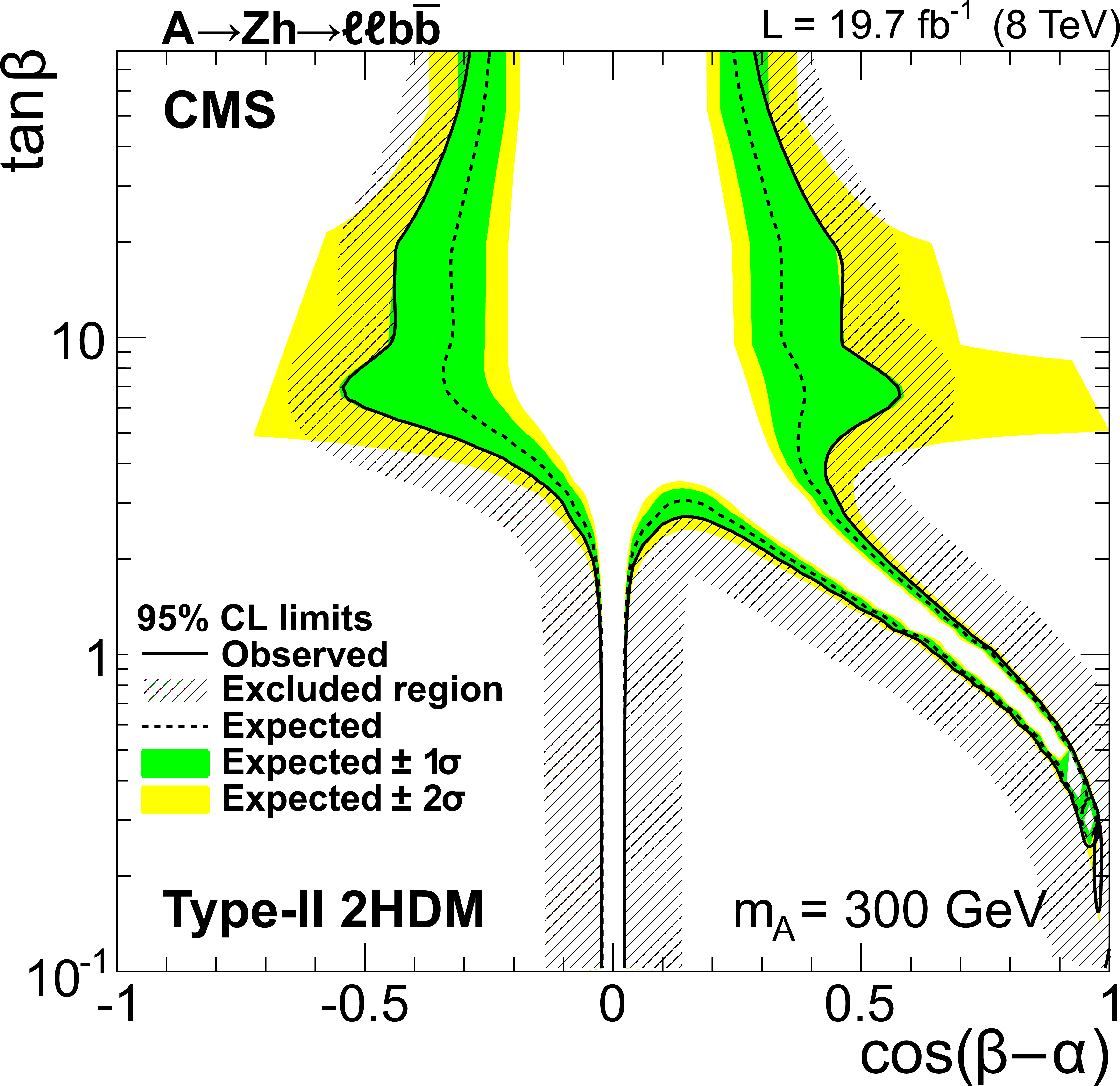
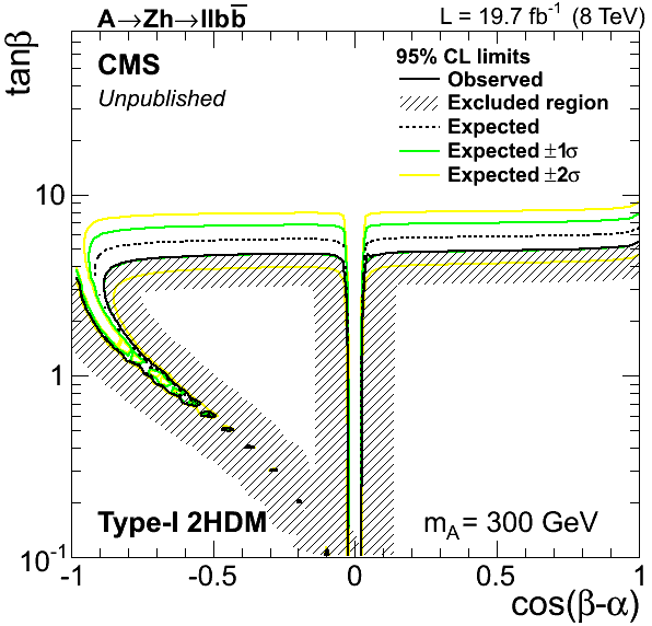
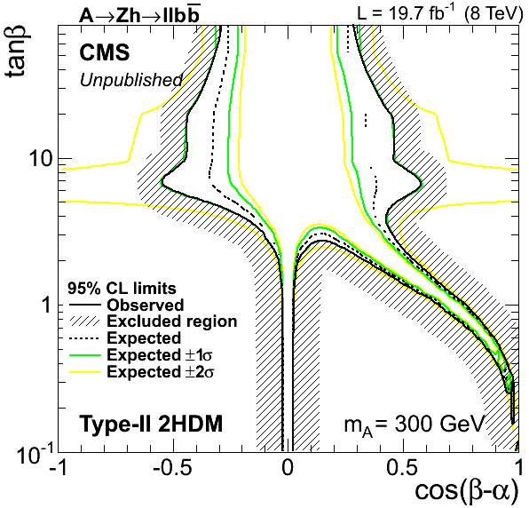
Observed and expected (together with ${\pm }1, 2\sigma $ uncertainty bands) exclusion limit for Type-I (a) and Type-II (b) models, as a function of $\tan{\beta}$ and $\cos(\beta -\alpha )$ . Contours are derived from the projection on the 2HDM parameter space for the $m_{\mathrm {A}}$ = 300 GeV signal hypothesis; the observed limit is close to $1 \sigma $ above the expected limit, as shown in Fig. 3. |
png pdf |
Figure 5-b:
Observed and expected (together with ${\pm }1, 2\sigma $ uncertainty bands) exclusion limit for Type-I (a) and Type-II (b) models, as a function of $\tan{\beta}$ and $\cos(\beta -\alpha )$ . Contours are derived from the projection on the 2HDM parameter space for the $m_{\mathrm {A}}$ = 300 GeV signal hypothesis; the observed limit is close to $1 \sigma $ above the expected limit, as shown in Fig. 3. |
| Summary |
| A search is presented for new physics in the extended Higgs sector, in signatures expected from decays of a pseudoscalar boson A into a Z boson and an SM-like h boson, with the Z boson decaying into $\ell^+ \ell^-$ ($\ell$ being either e or $\mu$) and the h boson into $\mathrm{ b \bar{b} } $. Different techniques are employed to increase the sensitivity to signal, exploiting the presence of the three resonances A, Z, and h to discriminate against standard model backgrounds. Upper limits at a 95% CL are set on the product of a narrow pseudoscalar boson cross section and branching fraction $\sigma_A \mathcal{B} ( A \to Zh \to \ell \ell \mathrm{ b \bar{b} } )$, which exclude 30 to 3 fb at the low and high ends of the 250-600 GeV mass range. Results are also presented as a function of the width of the A boson. Interpretations are given in the context of Type-I and Type-II 2HDM formulations, thereby reducing the parameter space for extensions of the standard model. |
| Additional Figures | |
png pdf |
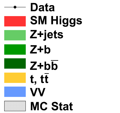
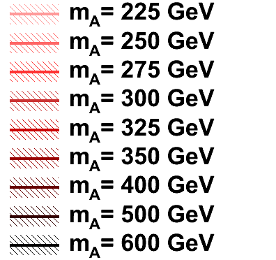
Additional Figure 1-a:
Legends for data and simulated background processes (a), and for the nine simulated signal mass points (b). |
png pdf |
Additional Figure 1-b:
Legends for data and simulated background processes (a), and for the nine simulated signal mass points (b). |
png pdf |
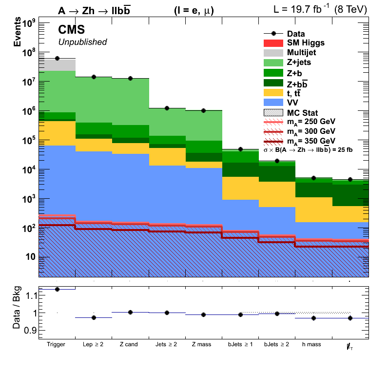
Additional Figure 2:
Data, simulated background and signal number of events after each selection cut, from trigger to the signal region. Signal templates are normalized to an arbitrary cross section $\sigma_{\mathrm{A}} \times \mathcal{B}(\mathrm{ A \to Zh \to \ell \ell b\bar{b} } ) =$ 25 fb. |
png pdf |
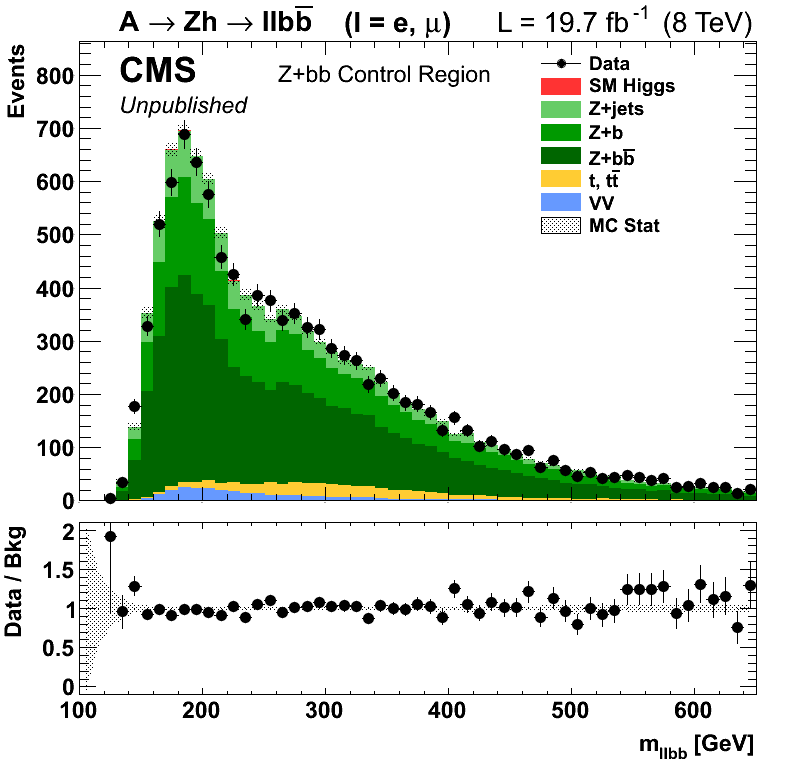
Additional Figure 3-a:
Control regions: Four-body $m_{\ell\ell \mathrm{bb}}$ invariant mass in the $\mathrm{ Z + b\bar{b} } $ control region (a) and dijet invariant mass in the $\mathrm{ t\overline{t} }$ control region (b). Scale factors are already applied. The lower plots show the ratio of data over simulated events, including the statistical uncertainties. |

png pdf |
Additional Figure 3-b:
Control regions: Four-body $m_{\ell\ell \mathrm{bb}}$ invariant mass in the $\mathrm{ Z + b\bar{b} } $ control region (a) and dijet invariant mass in the $\mathrm{ t\overline{t} }$ control region (b). Scale factors are already applied. The lower plots show the ratio of data over simulated events, including the statistical uncertainties. |
png pdf |
Additional Figure 4-a:
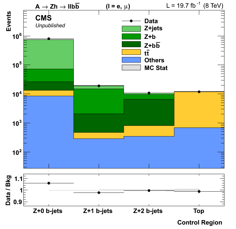
Scale factors: Data and background comparison in each one of the four control regions, before the likelihood fit and scale factors not applied (a); after the likelihood fit and scale factors already applied. |
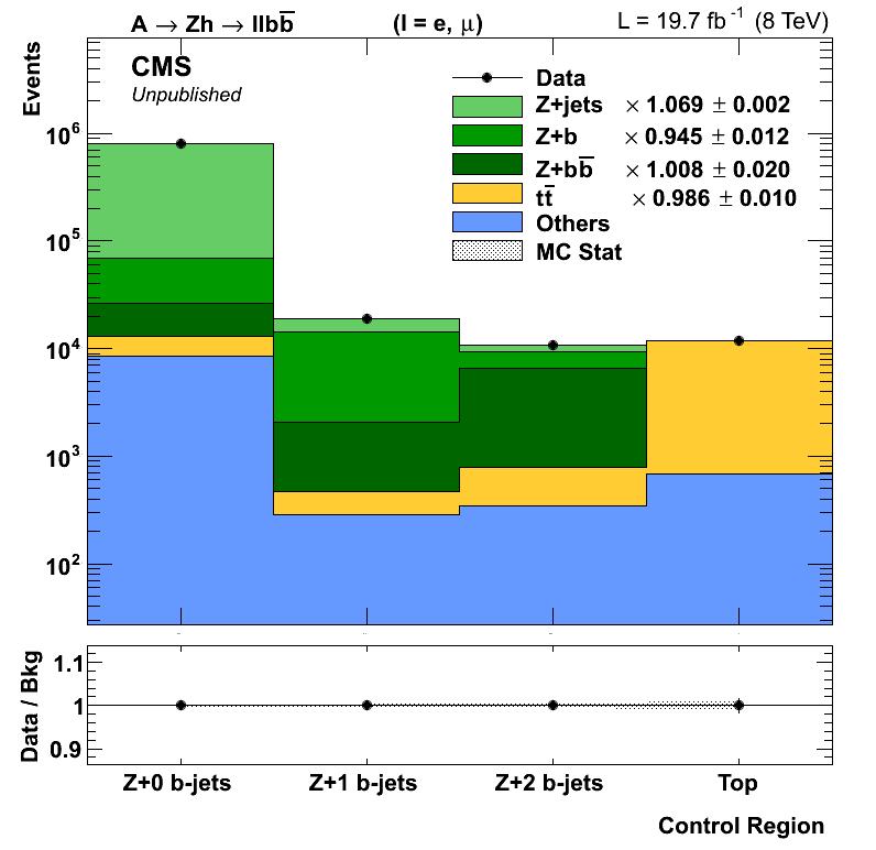
png pdf |
Additional Figure 4-b:
Scale factors: Data and background comparison in each one of the four control regions, before the likelihood fit and scale factors not applied (a); after the likelihood fit and scale factors already applied. |
png pdf |
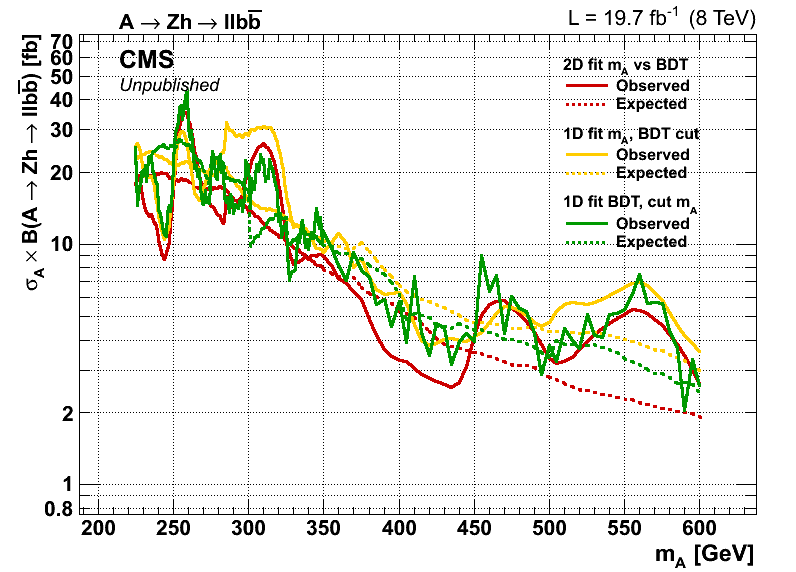
Additional Figure 5:
Observed and expected 95% CL upper limit on $\sigma_{\mathrm{A}} \times \mathcal{B}(\mathrm{ A \to Zh \to \ell \ell b\bar{b} })$, including all statistical and systematic uncertainties, for the 2D fit (red lines) and the two 1D cross-check analyses. The first one (yellow lines) consists of fitting the $m_{\ell\ell \mathrm{bb} }$ distribution, after selecting events in a signal-enriched region by applying a BDT > 0.8 selection. The second (green lines) relies on fits to the BDT distributions, after selecting events within the resolution of the signal $m_{\ell\ell \mathrm{bb} }$ peak. |
png pdf |
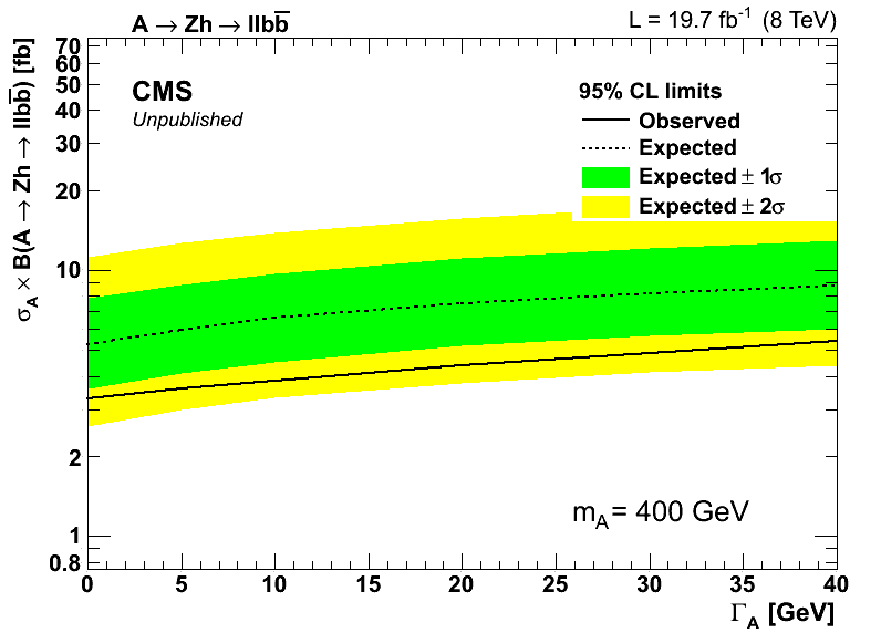
Additional Figure 6-a:
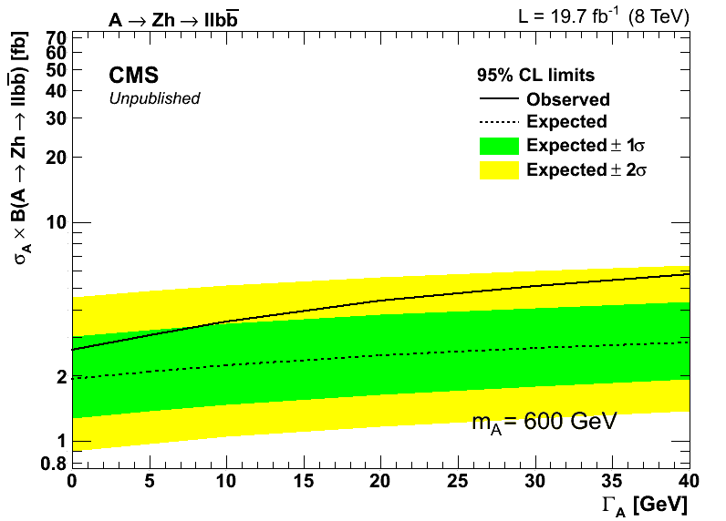
Observed and expected 95% CL upper limit on $\sigma_{\mathrm{A}} \times \mathcal{B}(\mathrm{ A \to Zh \to \ell \ell b\bar{b}})$ as a function of the width of the A boson, for $m_{\mathrm A} =$ 400 GeV (a) and $m_{\mathrm A} =$ 600 GeV (b). |
png pdf |
Additional Figure 6-b:
Observed and expected 95% CL upper limit on $\sigma_{\mathrm{A}} \times \mathcal{B}(\mathrm{ A \to Zh \to \ell \ell b\bar{b}})$ as a function of the width of the A boson, for $m_{\mathrm A} =$ 400 GeV (a) and $m_{\mathrm A} =$ 600 GeV (b). |
png pdf |
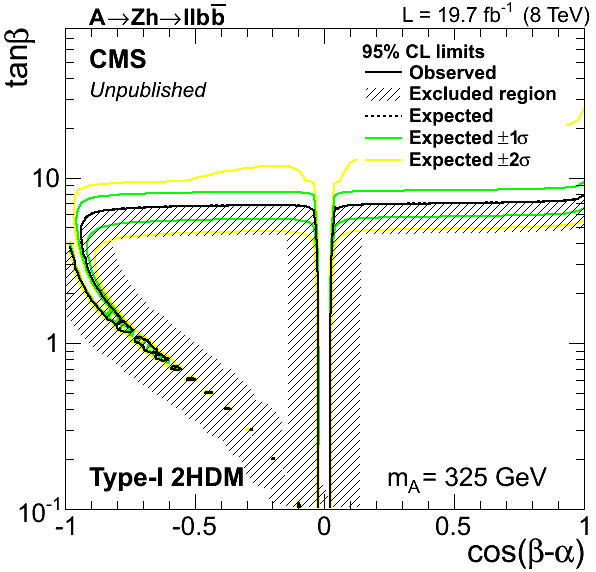
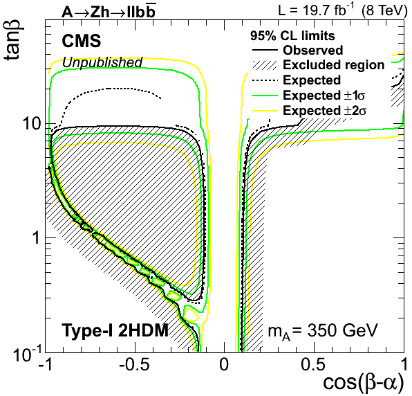
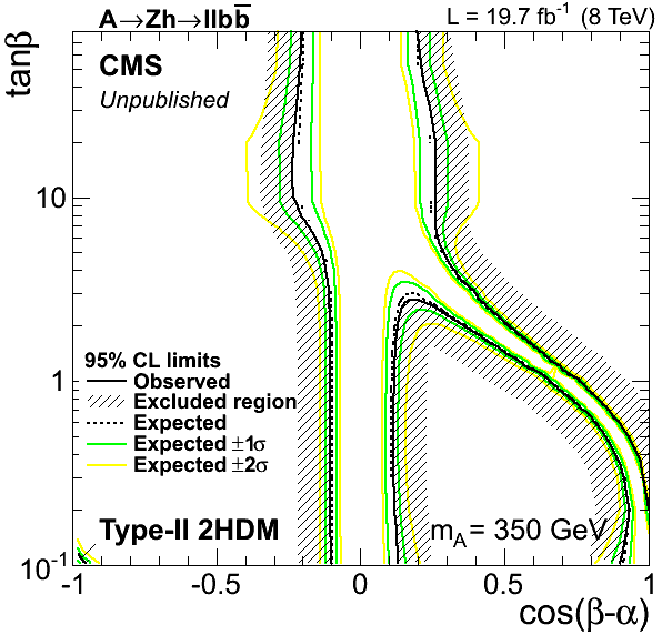
Additional Figure 7-a:
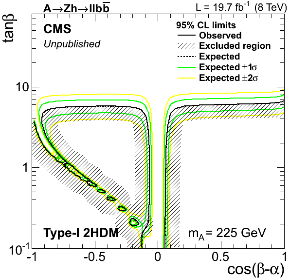
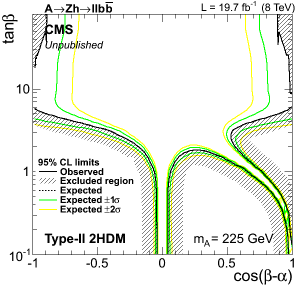
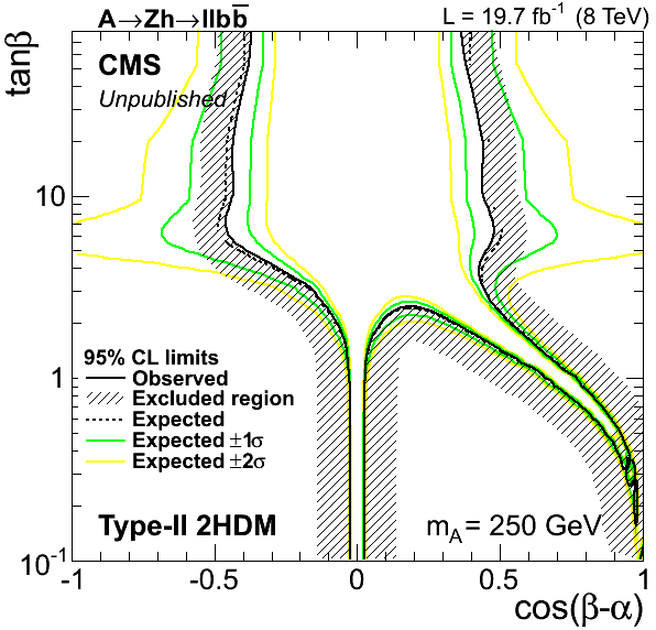
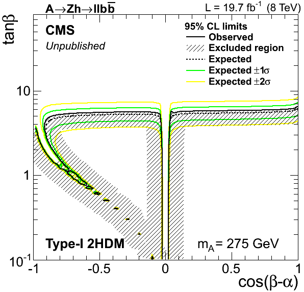
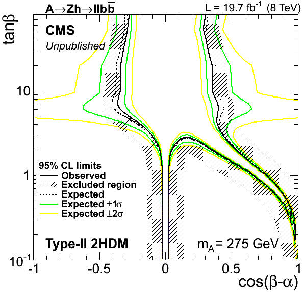
2HDM interpretation: Observed and expected (together with $\pm~1,~2\sigma$ uncertainty bands) exclusion limit for Type-I model (a, c, e, g, i, k) and Type-II model (b, d, f, h, j, l), as a function of $\tan \beta$ and $\cos(\beta-\alpha)$. Contours are derived from the projection on the 2HDM parameter space for the $m_A =$ 225 (a, b), 250 (c, d), 275 (e, f), 300 (g, h), 325 (i, j) and 350 (k, l) GeV signal hypothesis. |
png pdf |
Additional Figure 7-b:
2HDM interpretation: Observed and expected (together with $\pm~1,~2\sigma$ uncertainty bands) exclusion limit for Type-I model (a, c, e, g, i, k) and Type-II model (b, d, f, h, j, l), as a function of $\tan \beta$ and $\cos(\beta-\alpha)$. Contours are derived from the projection on the 2HDM parameter space for the $m_A =$ 225 (a, b), 250 (c, d), 275 (e, f), 300 (g, h), 325 (i, j) and 350 (k, l) GeV signal hypothesis. |

png pdf |
Additional Figure 7-c:
2HDM interpretation: Observed and expected (together with $\pm~1,~2\sigma$ uncertainty bands) exclusion limit for Type-I model (a, c, e, g, i, k) and Type-II model (b, d, f, h, j, l), as a function of $\tan \beta$ and $\cos(\beta-\alpha)$. Contours are derived from the projection on the 2HDM parameter space for the $m_A =$ 225 (a, b), 250 (c, d), 275 (e, f), 300 (g, h), 325 (i, j) and 350 (k, l) GeV signal hypothesis. |
png pdf |
Additional Figure 7-d:
2HDM interpretation: Observed and expected (together with $\pm~1,~2\sigma$ uncertainty bands) exclusion limit for Type-I model (a, c, e, g, i, k) and Type-II model (b, d, f, h, j, l), as a function of $\tan \beta$ and $\cos(\beta-\alpha)$. Contours are derived from the projection on the 2HDM parameter space for the $m_A =$ 225 (a, b), 250 (c, d), 275 (e, f), 300 (g, h), 325 (i, j) and 350 (k, l) GeV signal hypothesis. |
png pdf |
Additional Figure 7-e:
2HDM interpretation: Observed and expected (together with $\pm~1,~2\sigma$ uncertainty bands) exclusion limit for Type-I model (a, c, e, g, i, k) and Type-II model (b, d, f, h, j, l), as a function of $\tan \beta$ and $\cos(\beta-\alpha)$. Contours are derived from the projection on the 2HDM parameter space for the $m_A =$ 225 (a, b), 250 (c, d), 275 (e, f), 300 (g, h), 325 (i, j) and 350 (k, l) GeV signal hypothesis. |
png pdf |
Additional Figure 7-f:
2HDM interpretation: Observed and expected (together with $\pm~1,~2\sigma$ uncertainty bands) exclusion limit for Type-I model (a, c, e, g, i, k) and Type-II model (b, d, f, h, j, l), as a function of $\tan \beta$ and $\cos(\beta-\alpha)$. Contours are derived from the projection on the 2HDM parameter space for the $m_A =$ 225 (a, b), 250 (c, d), 275 (e, f), 300 (g, h), 325 (i, j) and 350 (k, l) GeV signal hypothesis. |
png pdf |
Additional Figure 7-g:
2HDM interpretation: Observed and expected (together with $\pm~1,~2\sigma$ uncertainty bands) exclusion limit for Type-I model (a, c, e, g, i, k) and Type-II model (b, d, f, h, j, l), as a function of $\tan \beta$ and $\cos(\beta-\alpha)$. Contours are derived from the projection on the 2HDM parameter space for the $m_A =$ 225 (a, b), 250 (c, d), 275 (e, f), 300 (g, h), 325 (i, j) and 350 (k, l) GeV signal hypothesis. |
png pdf |
Additional Figure 7-h:
2HDM interpretation: Observed and expected (together with $\pm~1,~2\sigma$ uncertainty bands) exclusion limit for Type-I model (a, c, e, g, i, k) and Type-II model (b, d, f, h, j, l), as a function of $\tan \beta$ and $\cos(\beta-\alpha)$. Contours are derived from the projection on the 2HDM parameter space for the $m_A =$ 225 (a, b), 250 (c, d), 275 (e, f), 300 (g, h), 325 (i, j) and 350 (k, l) GeV signal hypothesis. |
png pdf |
Additional Figure 7-i:
2HDM interpretation: Observed and expected (together with $\pm~1,~2\sigma$ uncertainty bands) exclusion limit for Type-I model (a, c, e, g, i, k) and Type-II model (b, d, f, h, j, l), as a function of $\tan \beta$ and $\cos(\beta-\alpha)$. Contours are derived from the projection on the 2HDM parameter space for the $m_A =$ 225 (a, b), 250 (c, d), 275 (e, f), 300 (g, h), 325 (i, j) and 350 (k, l) GeV signal hypothesis. |

png pdf |
Additional Figure 7-j:
2HDM interpretation: Observed and expected (together with $\pm~1,~2\sigma$ uncertainty bands) exclusion limit for Type-I model (a, c, e, g, i, k) and Type-II model (b, d, f, h, j, l), as a function of $\tan \beta$ and $\cos(\beta-\alpha)$. Contours are derived from the projection on the 2HDM parameter space for the $m_A =$ 225 (a, b), 250 (c, d), 275 (e, f), 300 (g, h), 325 (i, j) and 350 (k, l) GeV signal hypothesis. |
png pdf |
Additional Figure 7-k:
2HDM interpretation: Observed and expected (together with $\pm~1,~2\sigma$ uncertainty bands) exclusion limit for Type-I model (a, c, e, g, i, k) and Type-II model (b, d, f, h, j, l), as a function of $\tan \beta$ and $\cos(\beta-\alpha)$. Contours are derived from the projection on the 2HDM parameter space for the $m_A =$ 225 (a, b), 250 (c, d), 275 (e, f), 300 (g, h), 325 (i, j) and 350 (k, l) GeV signal hypothesis. |
png pdf |
Additional Figure 7-l:
2HDM interpretation: Observed and expected (together with $\pm~1,~2\sigma$ uncertainty bands) exclusion limit for Type-I model (a, c, e, g, i, k) and Type-II model (b, d, f, h, j, l), as a function of $\tan \beta$ and $\cos(\beta-\alpha)$. Contours are derived from the projection on the 2HDM parameter space for the $m_A =$ 225 (a, b), 250 (c, d), 275 (e, f), 300 (g, h), 325 (i, j) and 350 (k, l) GeV signal hypothesis. |
|
|
Compact Muon Solenoid LHC, CERN |
|

|

|

|

|

|