

Compact Muon Solenoid
LHC, CERN
| CMS-HIG-14-013 ; CERN-PH-EP-2015-042 | ||
| Search for resonant pair production of Higgs bosons decaying to two bottom quark-antiquark pairs in proton-proton collisions at 8 TeV | ||
| CMS Collaboration | ||
| 14 March 2015 | ||
| Phys. Lett. B 749 (2015) 560 | ||
| Abstract: A model-independent search for a narrow resonance produced in proton-proton collisions at $ \sqrt{s} $ = 8 TeV and decaying to a pair of 125 GeV Higgs bosons that in turn each decays into bottom quark-antiquark pairs is performed by the CMS experiment at the LHC. The analyzed data correspond to an integrated luminosity of 17.9 fb$ ^{−1} $. No evidence for a signal is observed. Upper limits at a 95% confidence level on the production cross section for such a resonance, in the mass range from 270 to 1100 GeV, are reported. Using these results, a radion with decay constant of 1 TeV and mass from 300 to 1100 GeV, and a Kaluza-Klein graviton with mass from 380 to 830 GeV are excluded at a 95% confidence level. | ||
| Links: e-print arXiv:1503.04114 [hep-ex] (PDF) ; CDS record ; inSPIRE record ; Public twiki page ; CADI line (restricted) ; | ||
| Figures | |

png pdf |
Figure 1:
Illustration of the SR, SB, VR and VS kinematic regions in the ($m_{{ {\mathrm {H}} }_1}$, $m_{{ {\mathrm {H}} }_2}$) plane used to motivate and validate the parametric model for the QCD multijet background. The quantities $m_{{ {\mathrm {H}} }_1}$ and $m_{{ {\mathrm {H}} }_2}$ are the two reconstructed Higgs boson masses. The distribution in data events after b-tagging and kinematic selections is shown with the SR blinded. |
png pdf |
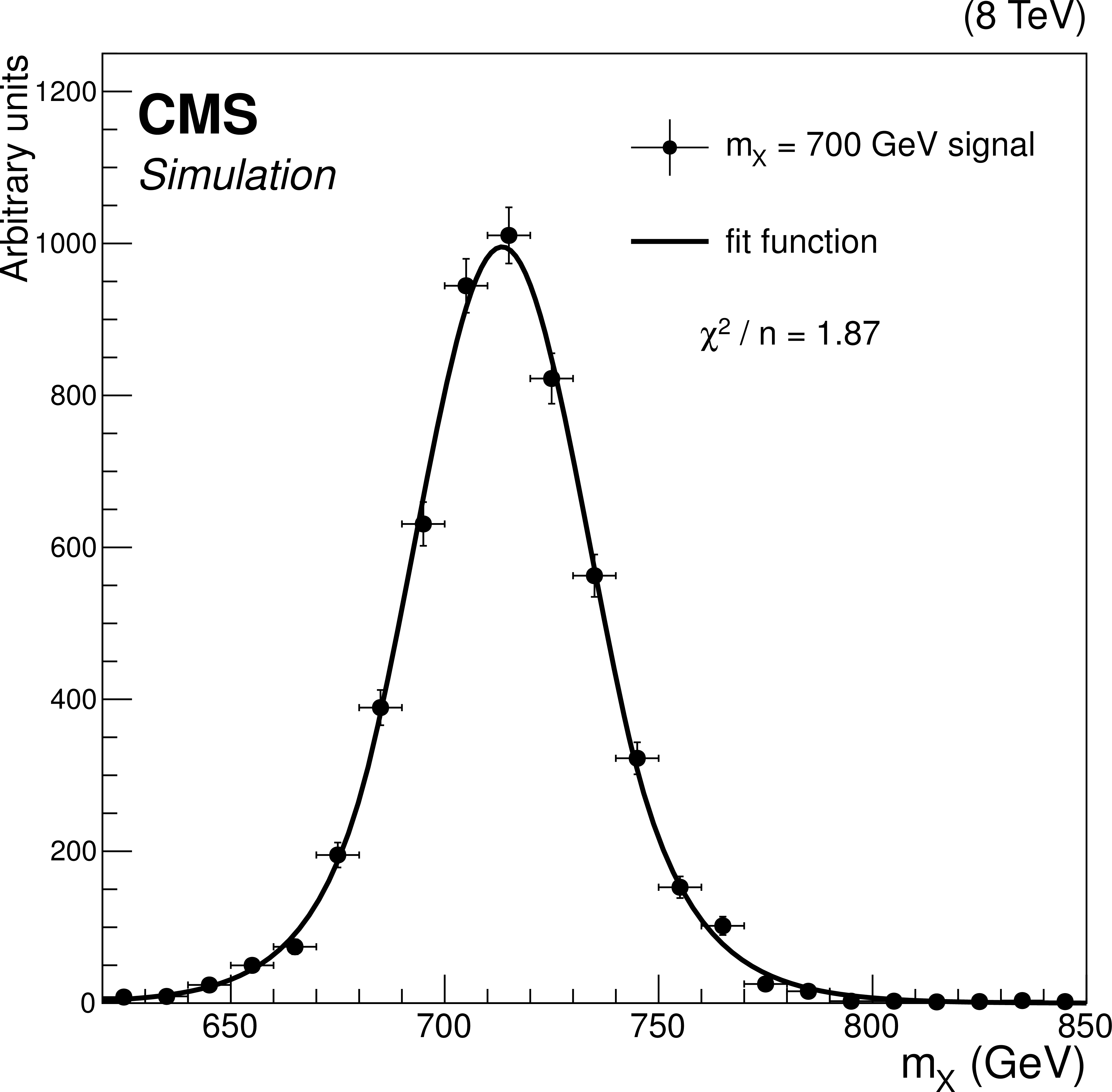
Figure 2:
A maximum likelihood fit to the $m_ {X} $ distribution of simulated signal events for the 700 GeV mass hypothesis. The distribution is fitted to a Gaussian core smoothly extended on both sides to exponential tails. Here $n$ is the number of degrees of freedom in the fit. |
png pdf |
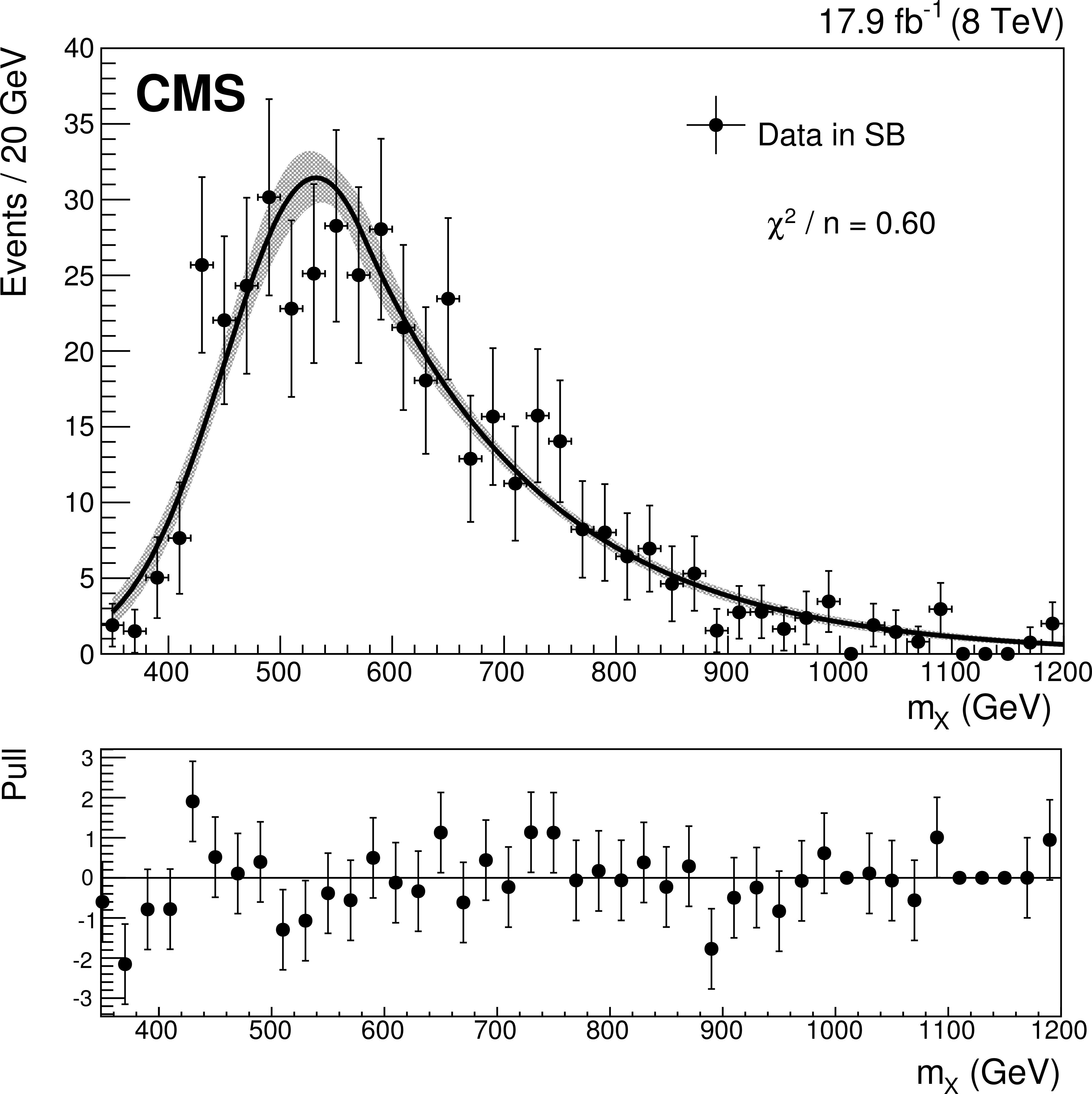
Figure 3-a:
The $m_ {X} $ distributions in data (after the ${\mathrm {t}\overline {\mathrm {t}}}$ background has been subtracted) in the SB of the HMR (a), the CR of the HMR (b), the VS of the LMR (c), and the VR of the LMR (d). The distributions are fitted to the GaussExp parametric model. The shaded regions correspond to $\pm $1$\sigma $ variations of this fit. Here $n$ is the number of degrees of freedom in each fit. The pull, for a given bin, is defined as the number of data events minus the value of the fit model, divided by the uncertainty on the number of data events. |
png pdf |
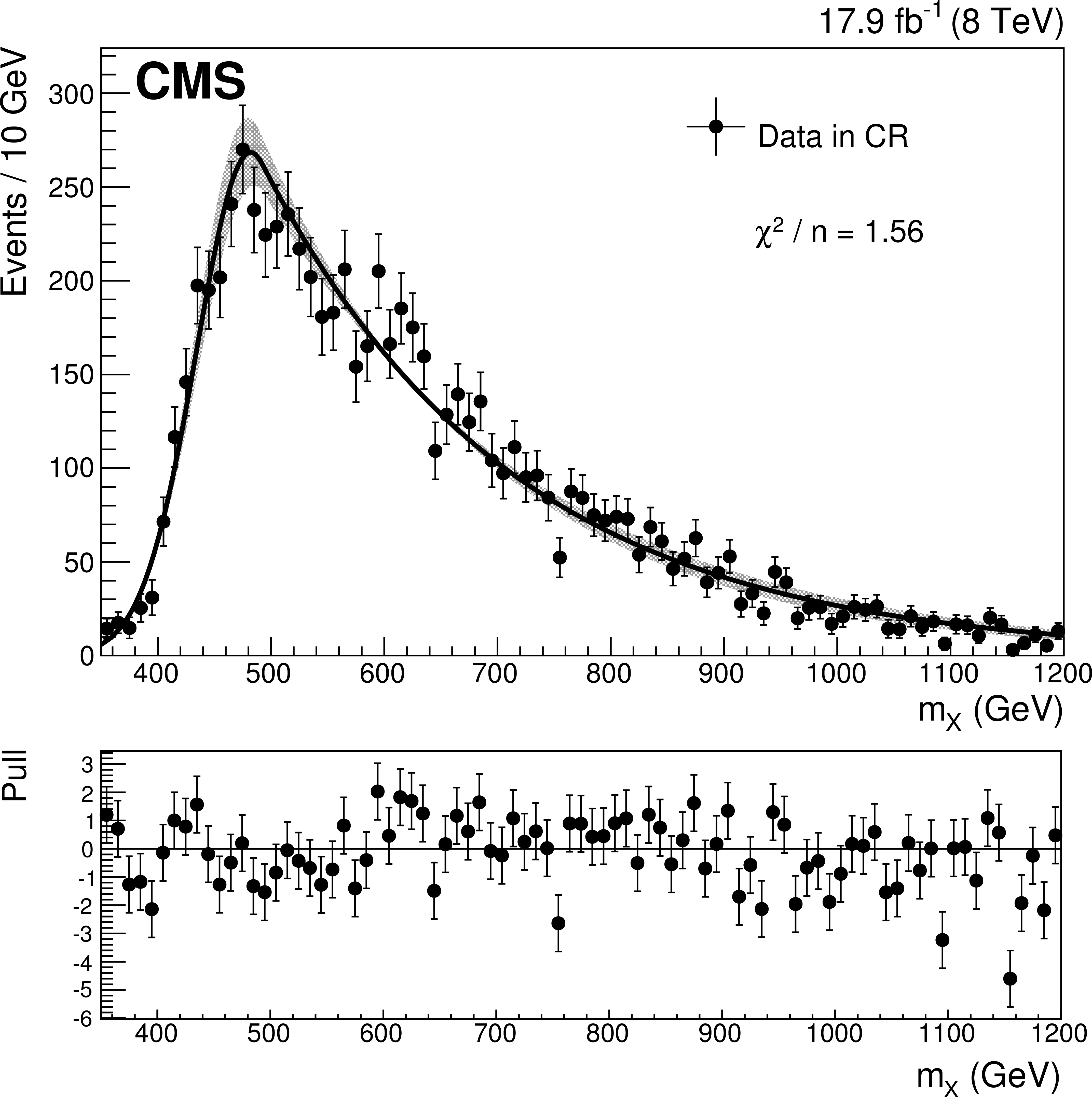
Figure 3-b:
The $m_ {X} $ distributions in data (after the ${\mathrm {t}\overline {\mathrm {t}}}$ background has been subtracted) in the SB of the HMR (a), the CR of the HMR (b), the VS of the LMR (c), and the VR of the LMR (d). The distributions are fitted to the GaussExp parametric model. The shaded regions correspond to $\pm $1$\sigma $ variations of this fit. Here $n$ is the number of degrees of freedom in each fit. The pull, for a given bin, is defined as the number of data events minus the value of the fit model, divided by the uncertainty on the number of data events. |
png pdf |
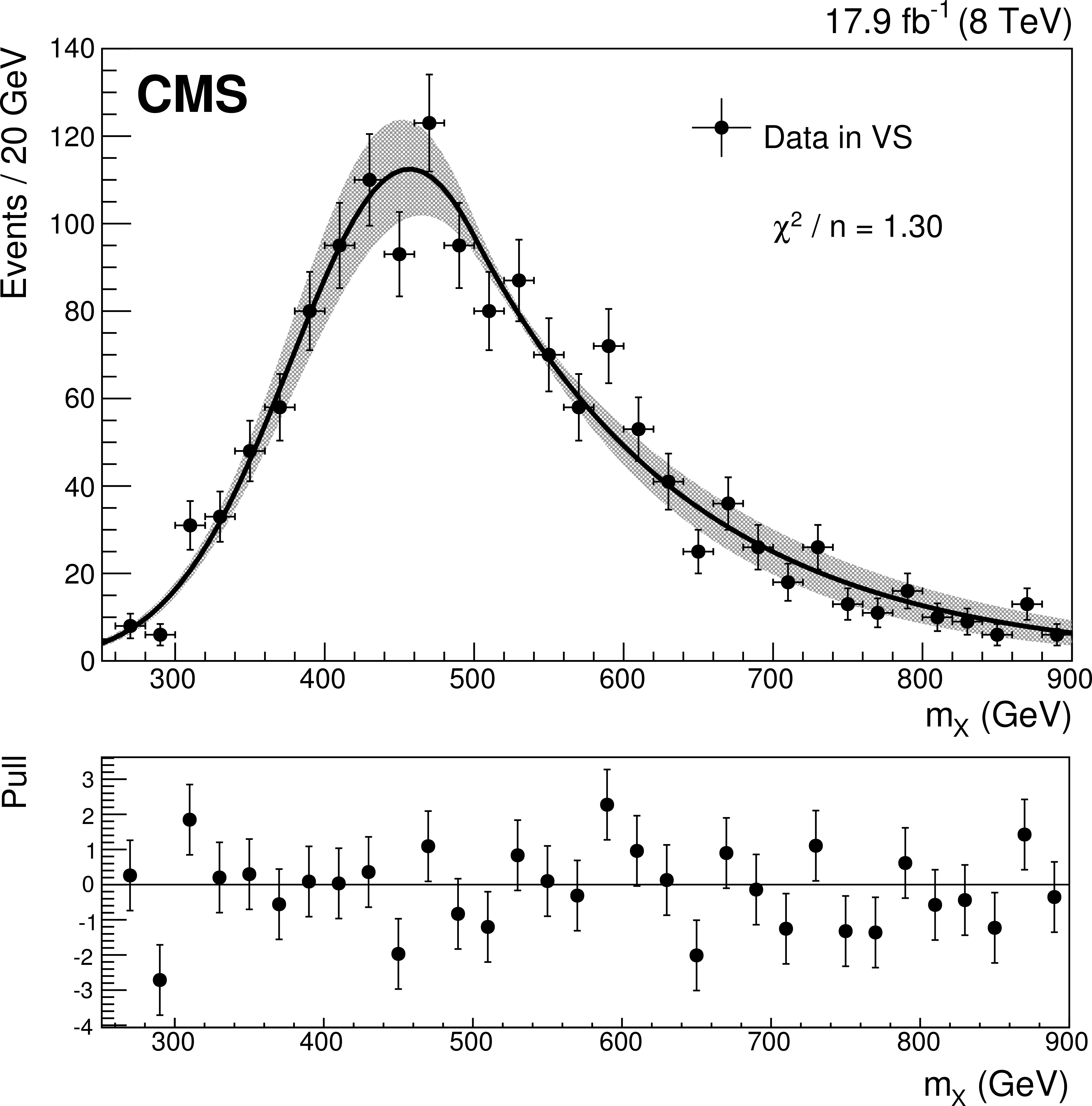
Figure 3-c:
The $m_ {X} $ distributions in data (after the ${\mathrm {t}\overline {\mathrm {t}}}$ background has been subtracted) in the SB of the HMR (a), the CR of the HMR (b), the VS of the LMR (c), and the VR of the LMR (d). The distributions are fitted to the GaussExp parametric model. The shaded regions correspond to $\pm $1$\sigma $ variations of this fit. Here $n$ is the number of degrees of freedom in each fit. The pull, for a given bin, is defined as the number of data events minus the value of the fit model, divided by the uncertainty on the number of data events. |

png pdf |
Figure 3-d:
The $m_ {X} $ distributions in data (after the ${\mathrm {t}\overline {\mathrm {t}}}$ background has been subtracted) in the SB of the HMR (a), the CR of the HMR (b), the VS of the LMR (c), and the VR of the LMR (d). The distributions are fitted to the GaussExp parametric model. The shaded regions correspond to $\pm $1$\sigma $ variations of this fit. Here $n$ is the number of degrees of freedom in each fit. The pull, for a given bin, is defined as the number of data events minus the value of the fit model, divided by the uncertainty on the number of data events. |
png pdf |
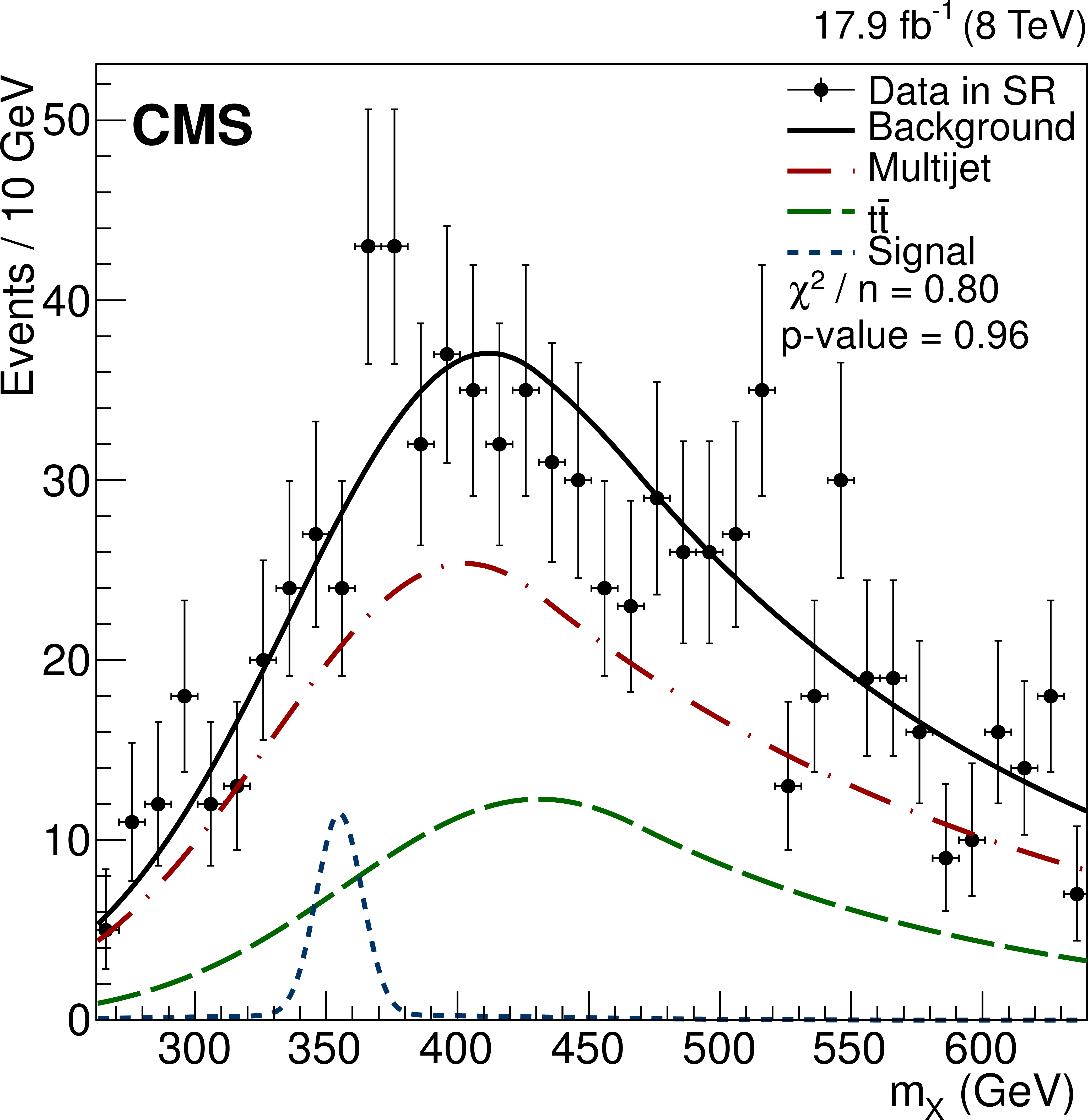
Figure 4-a:
The $m_ {X} $ distribution in data in the SR between 260 and 650 GeV of the LMR (a), between 400 and 900 GeV of the HMR (b), and between 600 and 1200 GeV in the HMR where one of the Higgs boson candidates has $ {p_{\mathrm {T}}} >$ 300 GeV (c). All distributions are fitted to the background-only hypothesis for illustration, showing the relative contributions of the QCD-multijet (dashed-dotted red) and ${\mathrm {t}\overline {\mathrm {t}}}$ (dashed green) processes. Also for illustration, we overlay the signal models of the spin-0 resonance (dotted blue) corresponding to mass hypotheses and production cross sections of 350 GeV and 653 fb for the LMR, 700 GeV and 17.6 fb for the HMR, and 900 GeV and 8.1 fb for the HMR with H $ {p_{\mathrm {T}}} >300$ GeV on their respective plots. These cross sections correspond to the observed upper limits, which are computed for signal mass hypotheses from 270 to 450 GeV in the LMR, from 450 to 730 GeV in the HMR, and from 730 to 1100 GeV in the HMR with H $ {p_{\mathrm {T}}} > $ 300 GeV . |
png pdf |
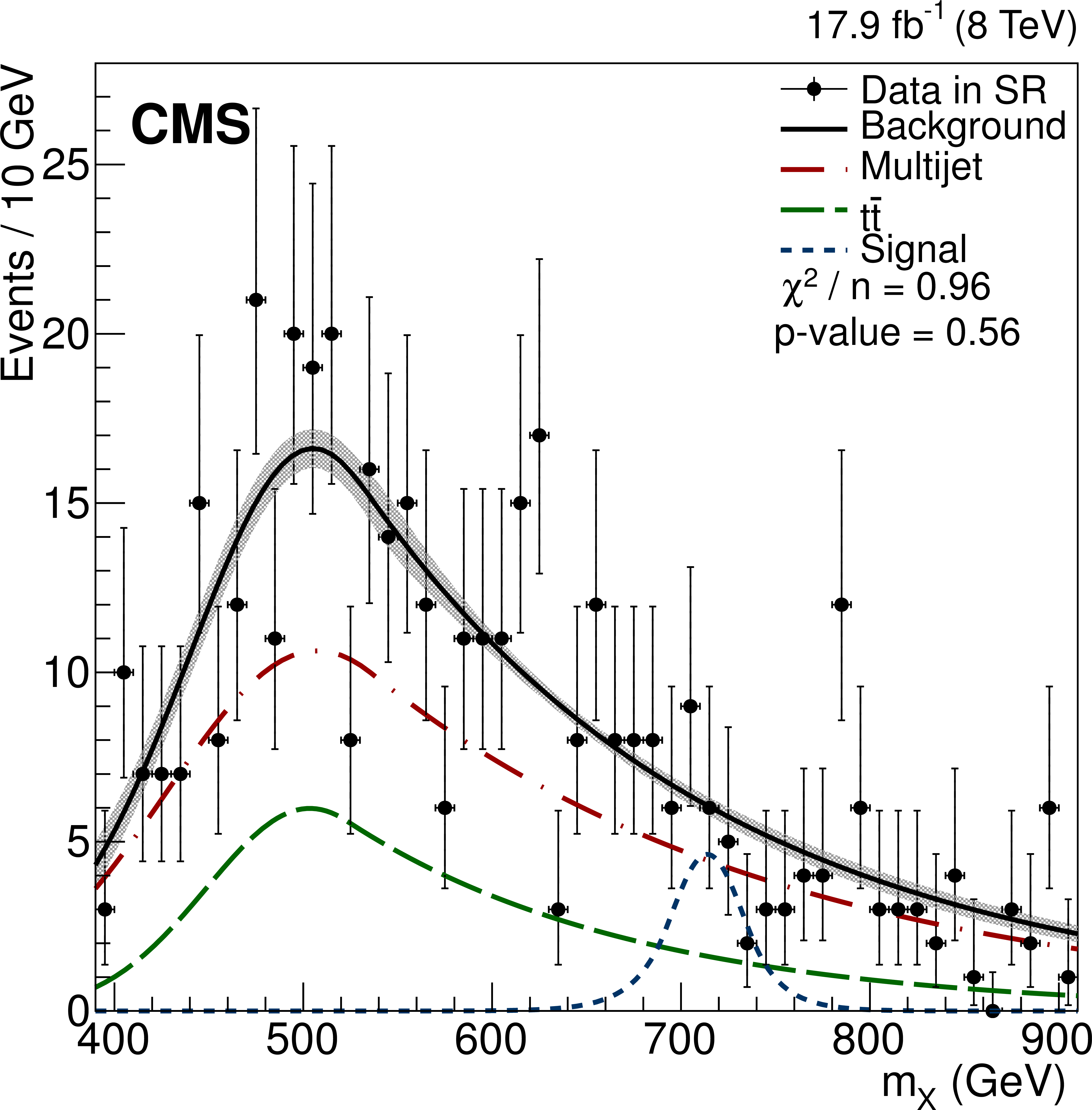
Figure 4-b:
The $m_ {X} $ distribution in data in the SR between 260 and 650 GeV of the LMR (a), between 400 and 900 GeV of the HMR (b), and between 600 and 1200 GeV in the HMR where one of the Higgs boson candidates has $ {p_{\mathrm {T}}} >$ 300 GeV (c). All distributions are fitted to the background-only hypothesis for illustration, showing the relative contributions of the QCD-multijet (dashed-dotted red) and ${\mathrm {t}\overline {\mathrm {t}}}$ (dashed green) processes. Also for illustration, we overlay the signal models of the spin-0 resonance (dotted blue) corresponding to mass hypotheses and production cross sections of 350 GeV and 653 fb for the LMR, 700 GeV and 17.6 fb for the HMR, and 900 GeV and 8.1 fb for the HMR with H $ {p_{\mathrm {T}}} >300$ GeV on their respective plots. These cross sections correspond to the observed upper limits, which are computed for signal mass hypotheses from 270 to 450 GeV in the LMR, from 450 to 730 GeV in the HMR, and from 730 to 1100 GeV in the HMR with H $ {p_{\mathrm {T}}} > $ 300 GeV . |
png pdf |
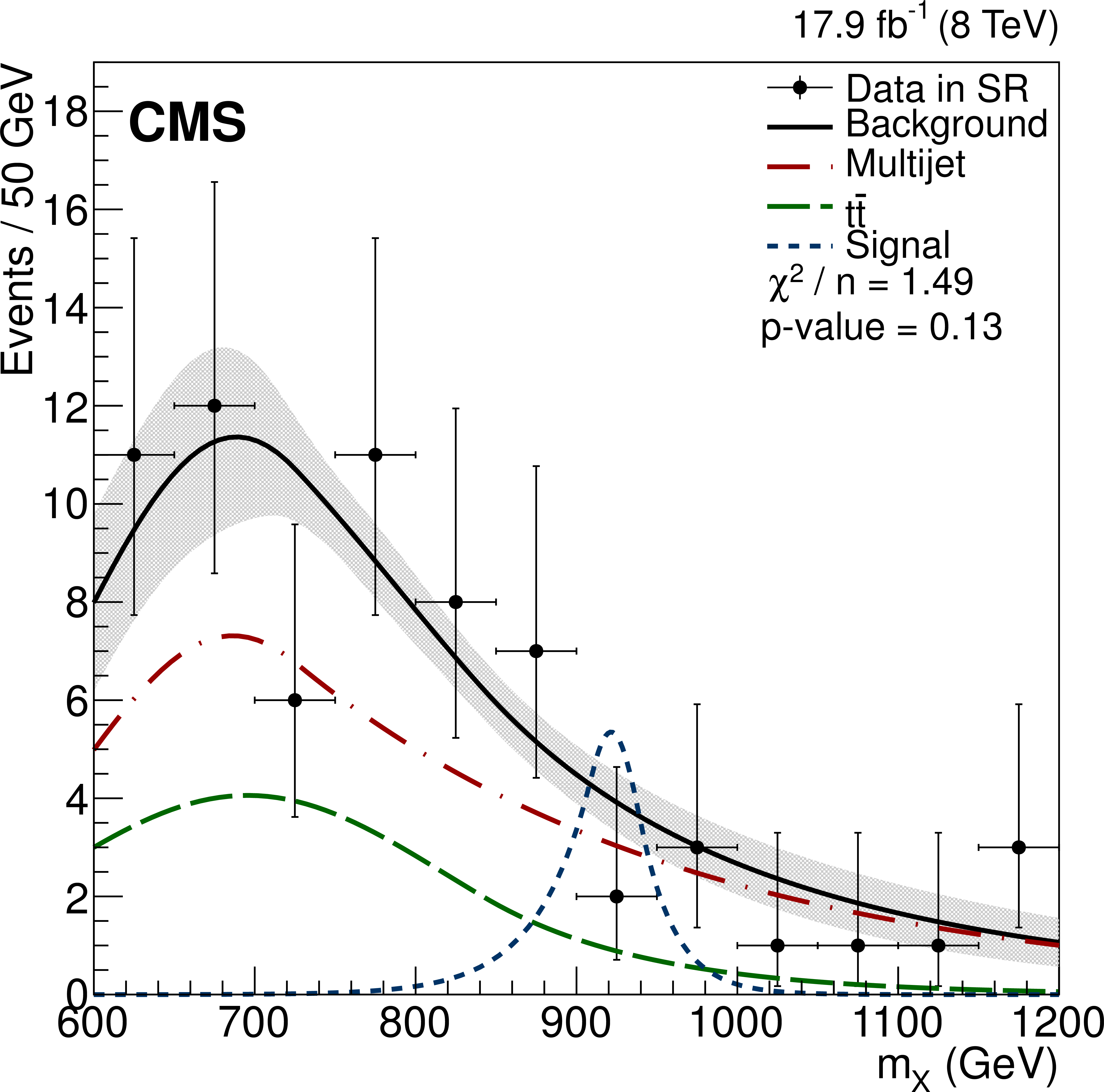
Figure 4-c:
The $m_ {X} $ distribution in data in the SR between 260 and 650 GeV of the LMR (a), between 400 and 900 GeV of the HMR (b), and between 600 and 1200 GeV in the HMR where one of the Higgs boson candidates has $ {p_{\mathrm {T}}} >$ 300 GeV (c). All distributions are fitted to the background-only hypothesis for illustration, showing the relative contributions of the QCD-multijet (dashed-dotted red) and ${\mathrm {t}\overline {\mathrm {t}}}$ (dashed green) processes. Also for illustration, we overlay the signal models of the spin-0 resonance (dotted blue) corresponding to mass hypotheses and production cross sections of 350 GeV and 653 fb for the LMR, 700 GeV and 17.6 fb for the HMR, and 900 GeV and 8.1 fb for the HMR with H $ {p_{\mathrm {T}}} >300$ GeV on their respective plots. These cross sections correspond to the observed upper limits, which are computed for signal mass hypotheses from 270 to 450 GeV in the LMR, from 450 to 730 GeV in the HMR, and from 730 to 1100 GeV in the HMR with H $ {p_{\mathrm {T}}} > $ 300 GeV . |
png pdf |
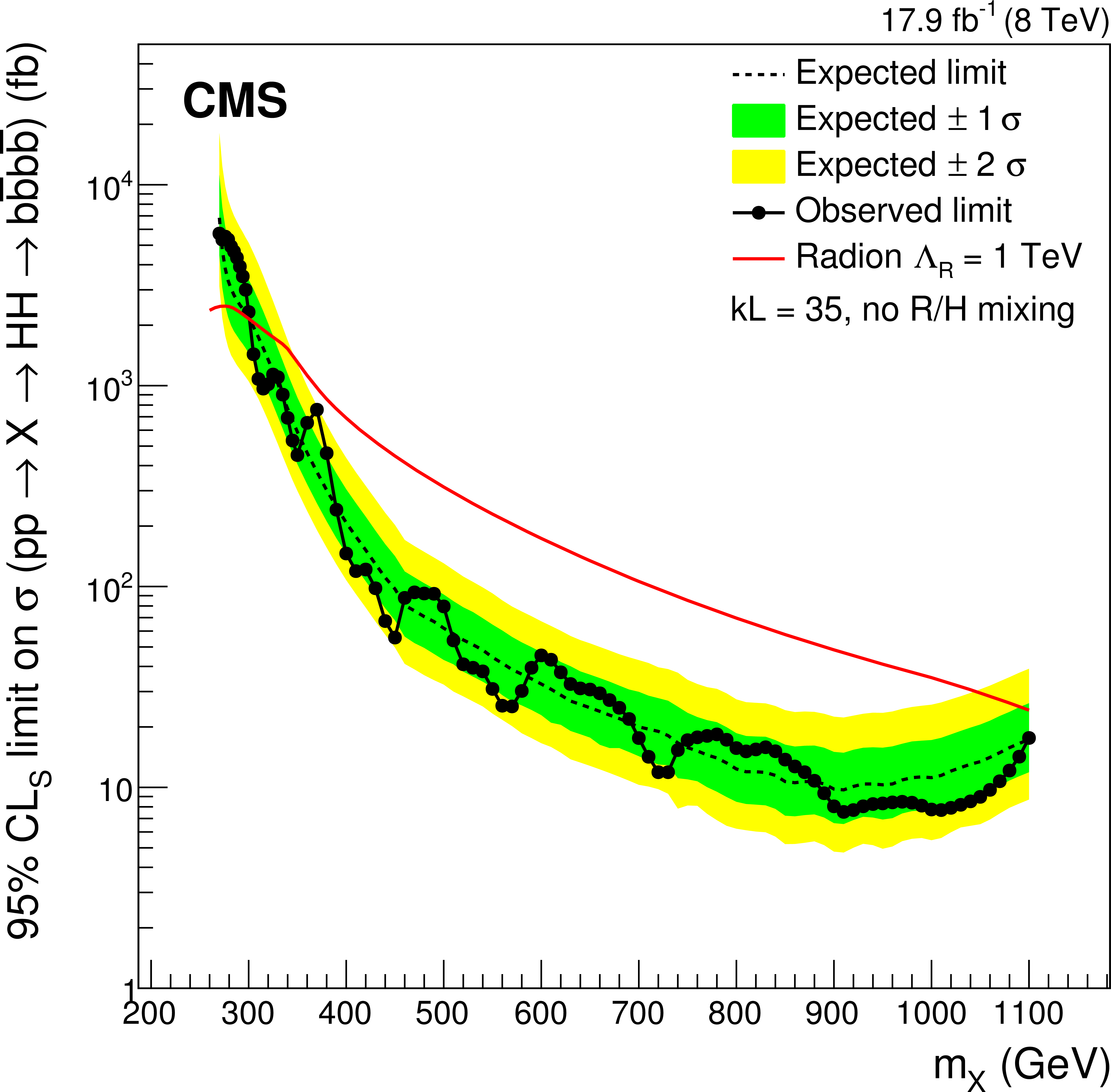
Figure 5-a:
The observed and expected upper limits on the cross section for $ { {\mathrm {p}} {\mathrm {p}}\to X \to {\mathrm {H}} ( { {\mathrm {b}} {\overline {\mathrm {b}}}} ) {\mathrm {H}} ( { {\mathrm {b}} {\overline {\mathrm {b}}}} )}\, $ at a 95% confidence level, where the resonance X has spin-0 (a) and spin-2 (b). The theoretical cross section for the RS1 radion, with $\Lambda _{R} = $ 1 TeV , $kL = 35$, and no radion-Higgs boson mixing, decaying to four b jets via Higgs bosons is overlaid on the left plot. The theoretical cross section for the first excitation of the KK-graviton for the same parameters is overlaid on the plot on Fig.5-b. |
png pdf |
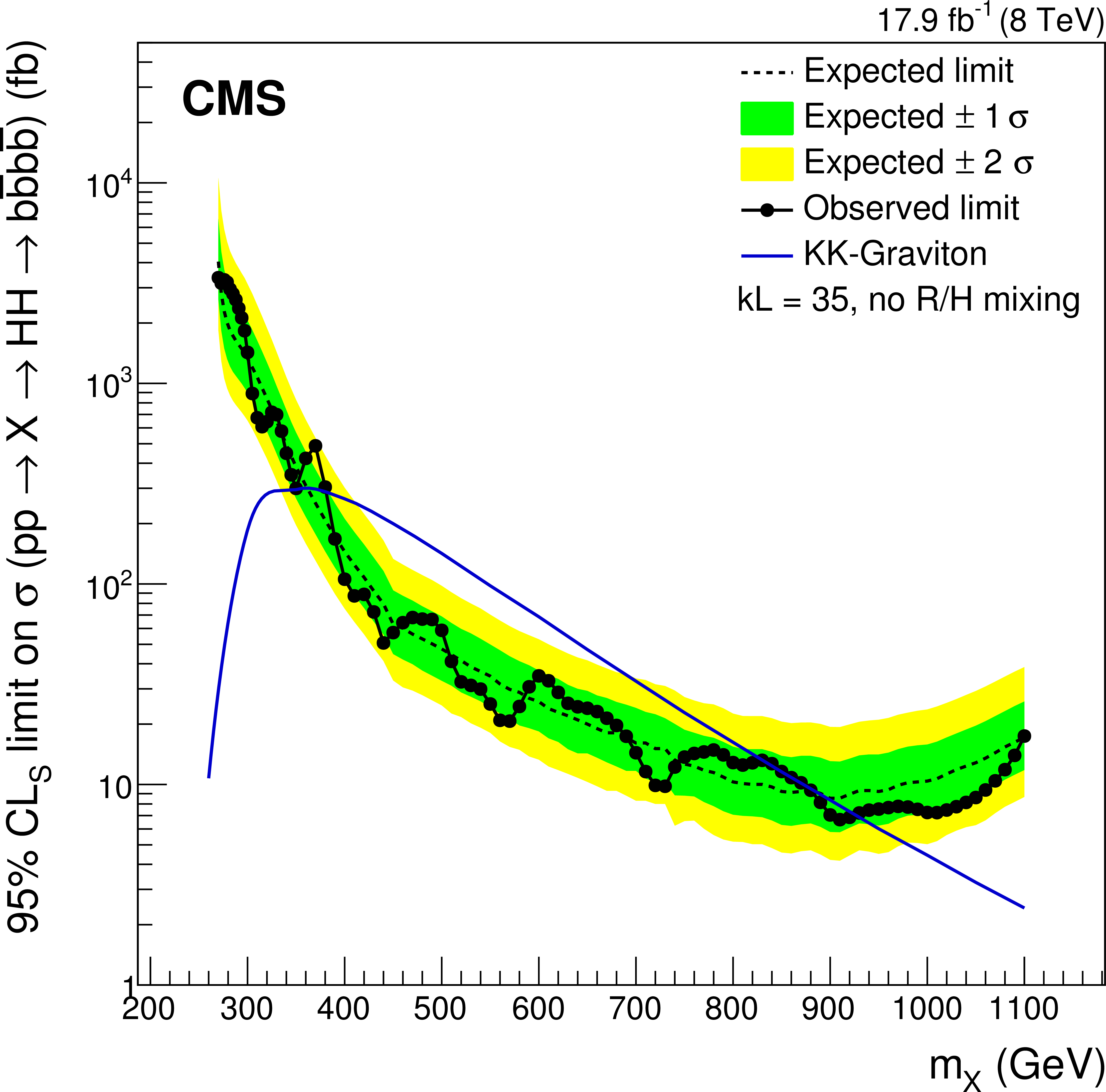
Figure 5-b:
The observed and expected upper limits on the cross section for $ { {\mathrm {p}} {\mathrm {p}}\to X \to {\mathrm {H}} ( { {\mathrm {b}} {\overline {\mathrm {b}}}} ) {\mathrm {H}} ( { {\mathrm {b}} {\overline {\mathrm {b}}}} )}\, $ at a 95% confidence level, where the resonance X has spin-0 (a) and spin-2 (b). The theoretical cross section for the RS1 radion, with $\Lambda _{R} = $ 1 TeV , $kL = 35$, and no radion-Higgs boson mixing, decaying to four b jets via Higgs bosons is overlaid on the left plot. The theoretical cross section for the first excitation of the KK-graviton for the same parameters is overlaid on the plot on Fig.5-b. |
|
|
Compact Muon Solenoid LHC, CERN |
|

|

|

|

|

|