

Compact Muon Solenoid
LHC, CERN
| CMS-HIG-14-017 ; CERN-PH-EP-2015-133 | ||
| Search for neutral MSSM Higgs bosons decaying into a pair of bottom quarks | ||
| CMS Collaboration | ||
| 28 June 2015 | ||
| Accepted for publication in J. High Energy Phys. J. High Energy Phys. 11 (2015) 071 | ||
| Abstract: A search for neutral Higgs bosons decaying into a $\mathrm{ b \bar{b}}$ quark pair and produced in association with at least one additional b quark is presented. This signature is sensitive to the Higgs sector of the minimal supersymmetric standard model (MSSM) with large values of the parameter $\tan \beta$. The analysis is based on data from proton-proton collisions at a center-of-mass energy of 8 TeV collected with the CMS detector at the LHC, corresponding to an integrated luminosity of 19.7 fb$^{-1}$. The results are combined with a previous analysis based on 7 TeV data. No signal is observed. Stringent upper limits on the cross section times branching fraction are derived for Higgs bosons with masses up to 900 GeV, and the results are interpreted within different MSSM benchmark scenarios, $m_{\mathrm{h}}^{\mathrm{max}}$, $m_{\mathrm{h}}^{\mathrm{mod+}}$, $m_{\mathrm{h}}^{\mathrm{mod-}}$, light-stau and light-stop. Observed 95\% confidence level upper limits on $\tan \beta$, ranging from 14 to 50, are obtained in the $m_{\mathrm{h}}^{\mathrm{mod+}}$ benchmark scenario. | ||
| Links: e-print arXiv:1506.08329 [hep-ex] (PDF) ; CDS record ; inSPIRE record ; HepData record ; CADI line (restricted) ; | ||
| Figures & Tables | Summary | Additional Figures | CMS Publications |
|---|
| Figures | |

png pdf |
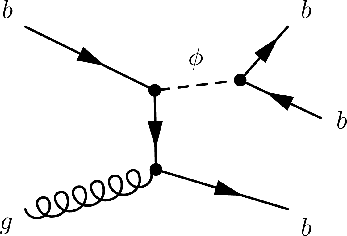
Figure 1-a:
Example Feynman diagrams of the signal processes. |

png pdf |
Figure 1-b:
Example Feynman diagrams of the signal processes. |
png pdf |
Figure 1-c:
Example Feynman diagrams of the signal processes. |
png pdf |
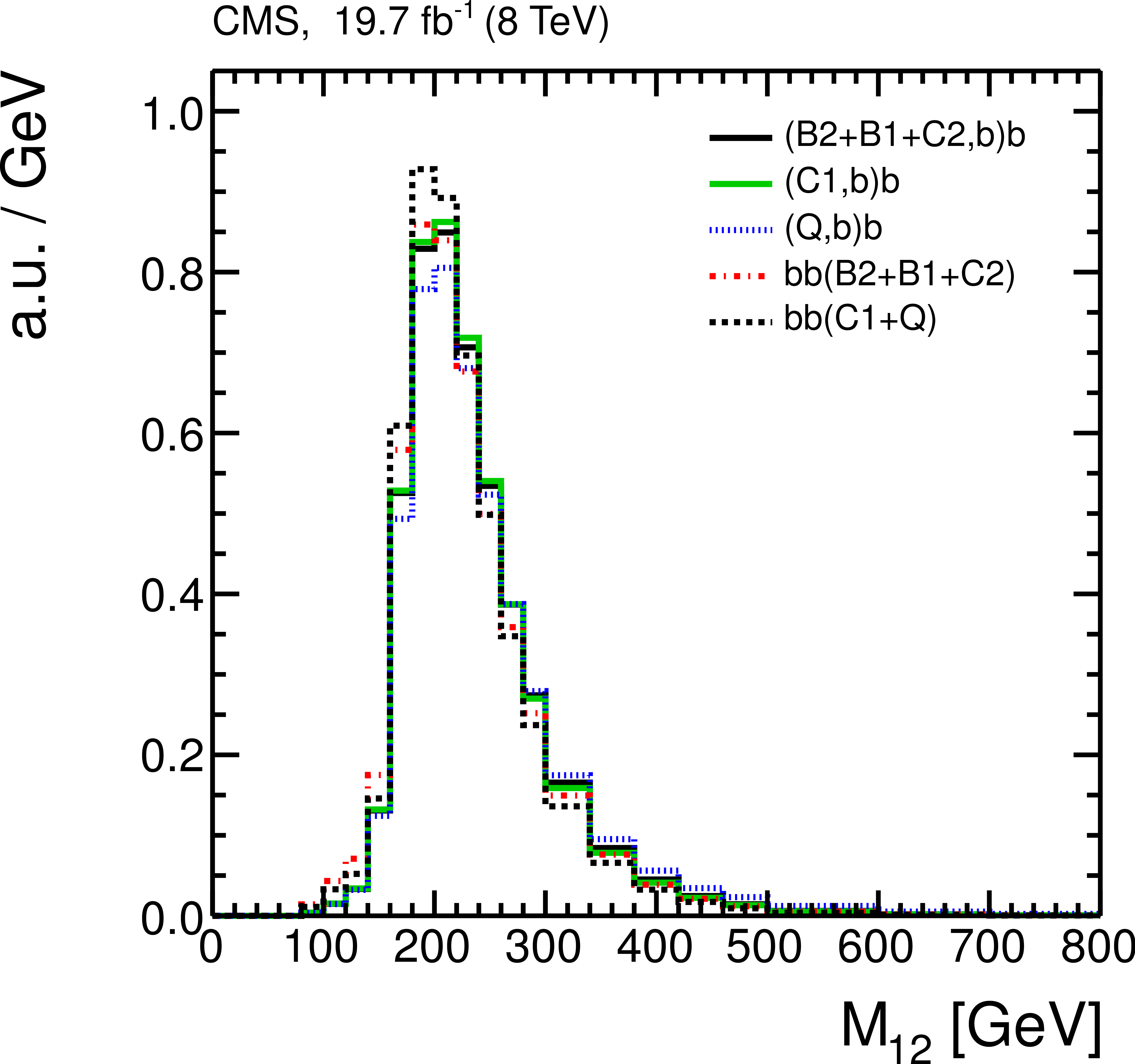
Figure 2-a:
Projections of $M_{12}$ (a) and $X_{123}$ (b) for the five background templates used in the fit. The vertical scale is shown in arbitrary units. |

png pdf |
Figure 2-b:
Projections of $M_{12}$ (a) and $X_{123}$ (b) for the five background templates used in the fit. The vertical scale is shown in arbitrary units. |

png pdf |
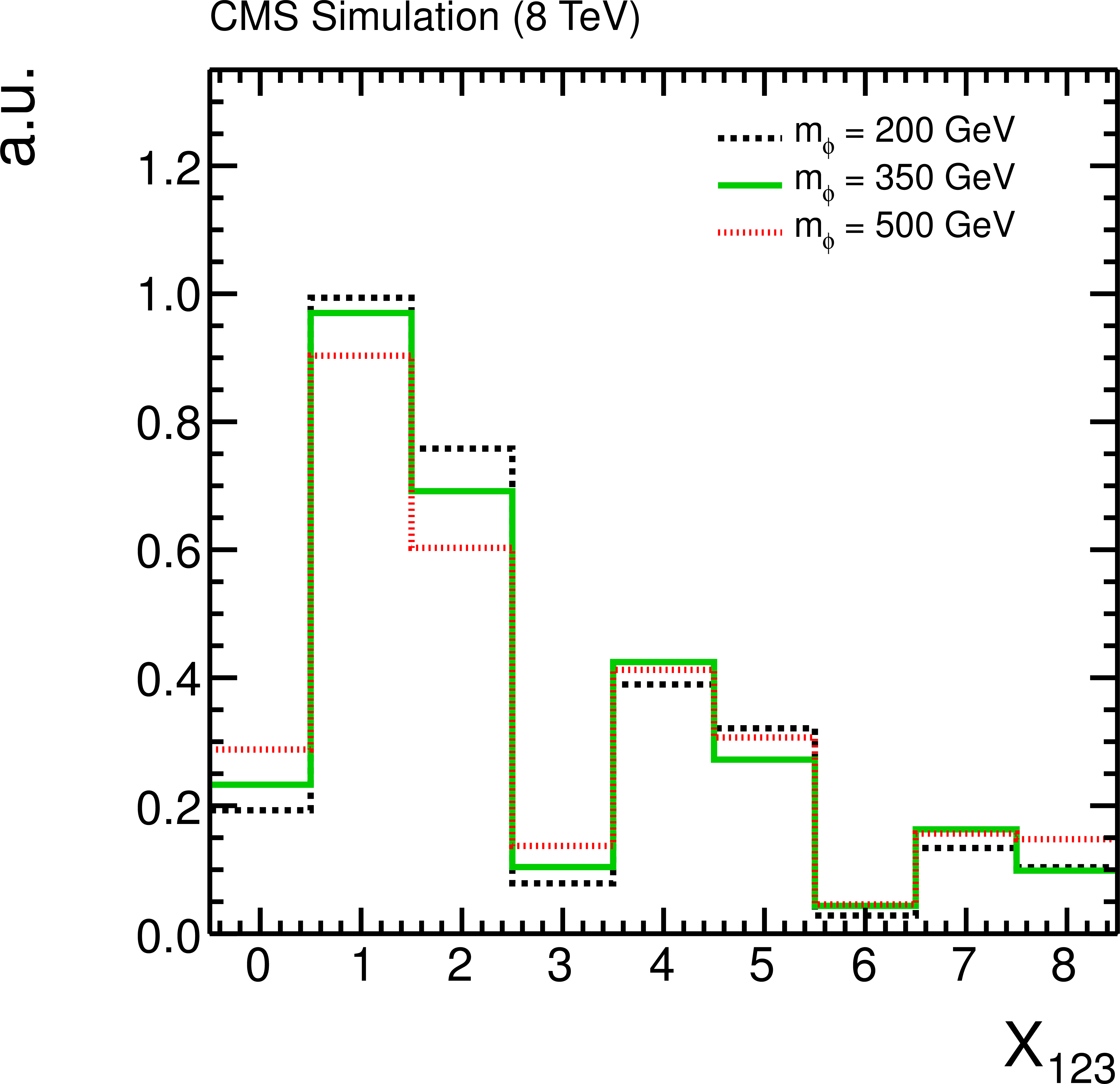
Figure 3-a:
The $M_{12}$ (a) and $X_{123}$ (b) projections of the signal templates for Higgs boson masses of $ {m_{\phi }} = $ 200, 350 and 500 GeV . The vertical scale is shown in arbitrary units. |
png pdf |
Figure 3-b:
The $M_{12}$ (a) and $X_{123}$ (b) projections of the signal templates for Higgs boson masses of $ {m_{\phi }} = $ 200, 350 and 500 GeV . The vertical scale is shown in arbitrary units. |

png pdf |
Figure 4-a:
Projections of the dijet mass $M_{12}$ (a) and event b-tag variable $X_{123}$ (b) in the triple-b-tag sample, together with the corresponding projections of the fitted background templates. The hatched area shows the total bin-by-bin background uncertainty of the templates prior to the fit, which takes into account the limited size of the double-b-tag sample and the uncertainties of the offline b-tag efficiencies and mistag rates. For illustration, the signal contribution expected in the $ {m_{ {\mathrm {h}} }^{\text {max}}} $ benchmark scenario of the MSSM with $ {m_{\mathrm {A}}} = $ 350 GeV , $\tan \beta =$ 30, and $\mu = $ +200 GeV is overlayed, scaled by a factor 10 for better readability. In addition, the ratio of data to the background estimate is shown at the bottom. |

png pdf |
Figure 4-b:
Projections of the dijet mass $M_{12}$ (a) and event b-tag variable $X_{123}$ (b) in the triple-b-tag sample, together with the corresponding projections of the fitted background templates. The hatched area shows the total bin-by-bin background uncertainty of the templates prior to the fit, which takes into account the limited size of the double-b-tag sample and the uncertainties of the offline b-tag efficiencies and mistag rates. For illustration, the signal contribution expected in the $ {m_{ {\mathrm {h}} }^{\text {max}}} $ benchmark scenario of the MSSM with $ {m_{\mathrm {A}}} = $ 350 GeV , $\tan \beta =$ 30, and $\mu = $ +200 GeV is overlayed, scaled by a factor 10 for better readability. In addition, the ratio of data to the background estimate is shown at the bottom. |

png pdf |
Figure 5-a:
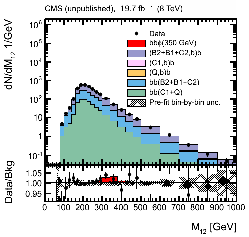
Results from the combined fit of signal and background templates in the triple-b-tag sample, at the 350 GeV mass point. The left plot shows the projections of the dijet mass $M_{12}$, the right plot the projections of the event b-tag variable $X_{123}$. The red graph represents the fitted Higgs signal contribution. The hatched area shows the total bin-by-bin background uncertainty of the templates prior to the fit, which takes into account the limited size of the double-b-tag sample and the uncertainties of the offline b-tag efficiencies and mistag rates. In addition, the ratio of data to the background estimate is shown at the bottom. |

png pdf |
Figure 5-b:
Results from the combined fit of signal and background templates in the triple-b-tag sample, at the 350 GeV mass point. The left plot shows the projections of the dijet mass $M_{12}$, the right plot the projections of the event b-tag variable $X_{123}$. The red graph represents the fitted Higgs signal contribution. The hatched area shows the total bin-by-bin background uncertainty of the templates prior to the fit, which takes into account the limited size of the double-b-tag sample and the uncertainties of the offline b-tag efficiencies and mistag rates. In addition, the ratio of data to the background estimate is shown at the bottom. |

png pdf |
Figure 6:
Expected and observed upper limits at 95% CL on $\sigma ( {\mathrm {pp} \to {\mathrm {b}} \phi +\mathrm {X})\mathcal {B}(\phi \to {\mathrm {b}} {\overline {\mathrm {b}}}} )$ as a function of $ {m_{\phi }} $, where $\phi $ denotes a generic neutral Higgs-like state. |

png pdf |
Figure 7-a:
Expected and observed upper limits at 95% CL for the MSSM parameter $\tan \beta $ versus $ {m_{\mathrm {A}}} $ in the $ {m_{ {\mathrm {h}} }^{\text {max}}} $ benchmark scenario with $\mu =$ +200 GeV. The excluded parameter space (observed limit) is indicated by the shaded area. Regions where the mass of neither of the CP-even MSSM Higgs bosons h or H is compatible with the discovered Higgs boson of 125 GeV within a range of 3 GeV are marked by the hatched areas. The left plot shows the result obtained with the 8 TeV data only, the right plot shows the result obtained after a combination with the 7 TeV data. For comparison, the expected limit of the 7 TeV data analysis is overlayed. |

png pdf |
Figure 7-b:
Expected and observed upper limits at 95% CL for the MSSM parameter $\tan \beta $ versus $ {m_{\mathrm {A}}} $ in the $ {m_{ {\mathrm {h}} }^{\text {max}}} $ benchmark scenario with $\mu =$ +200 GeV. The excluded parameter space (observed limit) is indicated by the shaded area. Regions where the mass of neither of the CP-even MSSM Higgs bosons h or H is compatible with the discovered Higgs boson of 125 GeV within a range of 3 GeV are marked by the hatched areas. The left plot shows the result obtained with the 8 TeV data only, the right plot shows the result obtained after a combination with the 7 TeV data. For comparison, the expected limit of the 7 TeV data analysis is overlayed. |

png pdf |
Figure 8-a:
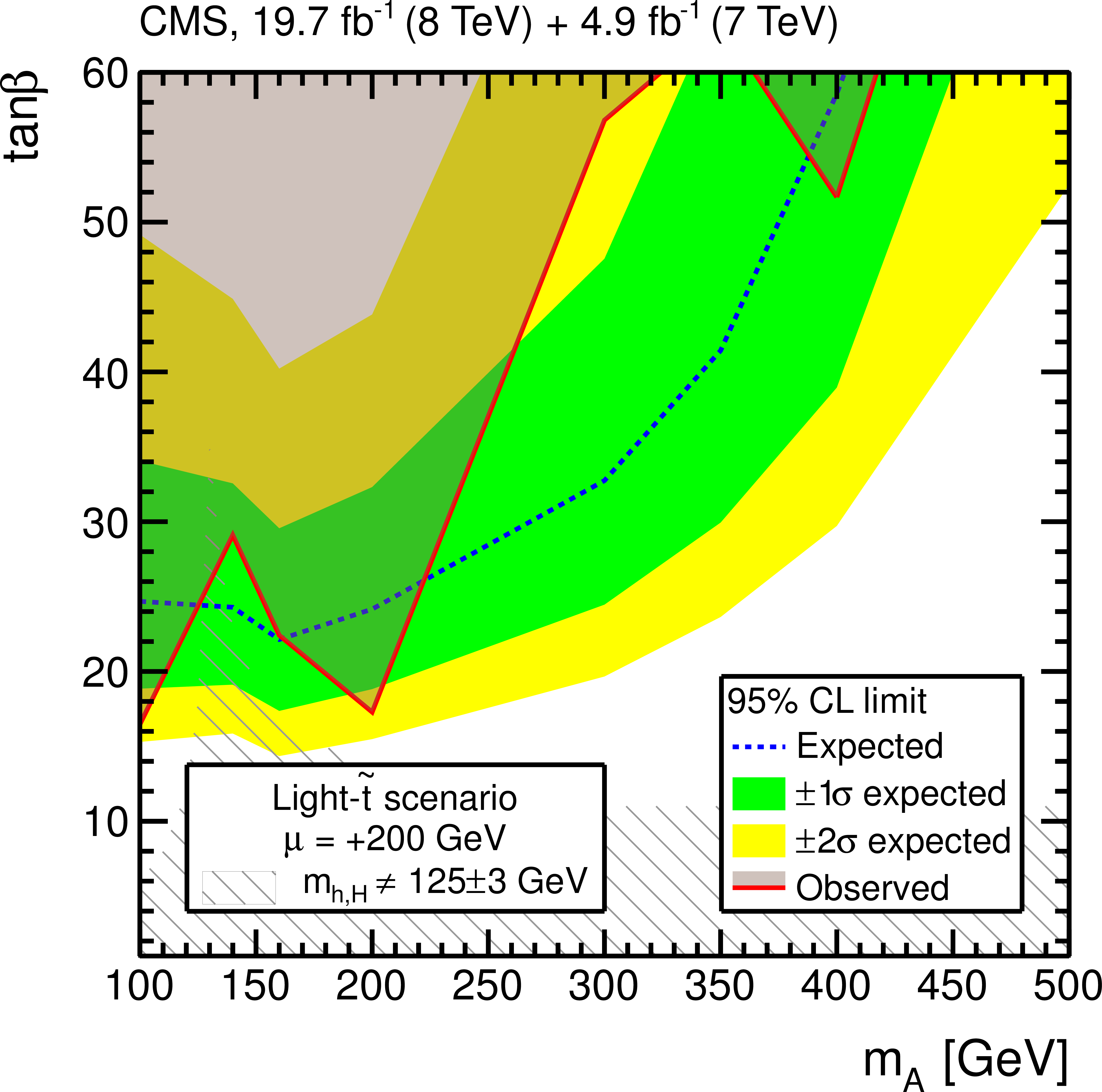
Expected and observed upper limits at 95% CL for the MSSM parameter $\tan\beta $ versus $ {m_{\mathrm {A}}} $ in the $ {m_{ {\mathrm {h}} }^{\text {mod+}}} $, $ {m_{ {\mathrm {h}} }^{\text {mod--}}} $, light-stop, and light-stau benchmark scenarios with $\mu = $+200 GeV. |
png pdf |
Figure 8-b:
Expected and observed upper limits at 95% CL for the MSSM parameter $\tan\beta $ versus $ {m_{\mathrm {A}}} $ in the $ {m_{ {\mathrm {h}} }^{\text {mod+}}} $, $ {m_{ {\mathrm {h}} }^{\text {mod--}}} $, light-stop, and light-stau benchmark scenarios with $\mu = $+200 GeV. |
png pdf |
Figure 8-c:
Expected and observed upper limits at 95% CL for the MSSM parameter $\tan\beta $ versus $ {m_{\mathrm {A}}} $ in the $ {m_{ {\mathrm {h}} }^{\text {mod+}}} $, $ {m_{ {\mathrm {h}} }^{\text {mod--}}} $, light-stop, and light-stau benchmark scenarios with $\mu = $+200 GeV. |

png pdf |
Figure 8-d:
Expected and observed upper limits at 95% CL for the MSSM parameter $\tan\beta $ versus $ {m_{\mathrm {A}}} $ in the $ {m_{ {\mathrm {h}} }^{\text {mod+}}} $, $ {m_{ {\mathrm {h}} }^{\text {mod--}}} $, light-stop, and light-stau benchmark scenarios with $\mu = $+200 GeV. |

png pdf |
Figure 9-a:
Expected and observed upper limits at 95% CL for the MSSM parameter $\tan \beta $ versus ${m_{\mathrm {A}}} $ for four different values of the higgsino mass parameter $\mu $ (a) and versus $\mu $ for three different values of $ {m_{\mathrm {A}}} $ (b) in the $ {m_{ {\mathrm {h}} }^{\text {mod+}}} $ scenario. |

png pdf |
Figure 9-b:
Expected and observed upper limits at 95% CL for the MSSM parameter $\tan \beta $ versus ${m_{\mathrm {A}}} $ for four different values of the higgsino mass parameter $\mu $ (a) and versus $\mu $ for three different values of $ {m_{\mathrm {A}}} $ (b) in the $ {m_{ {\mathrm {h}} }^{\text {mod+}}} $ scenario. |

png pdf |
Figure 10:
The signal efficiency as a function of the Higgs boson mass $m_\phi $, for a center-of-mass energy of 8 TeV. |
| Tables | |

png pdf |
Table 1:
Left: Definition of the index $B_j$ according to the value of the secondary vertex mass sum of the jet. Right: Definition of the values of the combined event b tagging estimator $X_{123}$ for all combinations of the secondary vertex mass sum indices $B_1$, $B_2$, and $B_3$. |
png pdf |
Table 2:
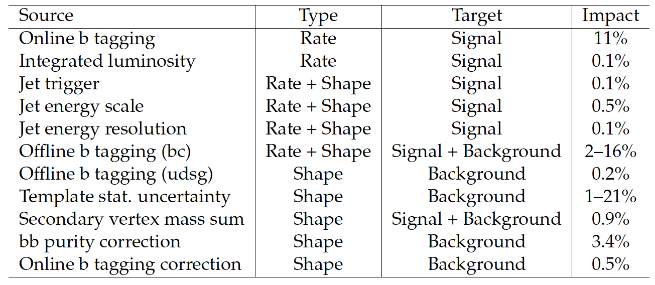
Systematic uncertainties and their relative impact on the expected limit. The values represent an average over the mass range from 100-900 GeV, except for the template statistical and the offline b tagging (bc) uncertainties, where ranges are given. |
png pdf |
Table 3:
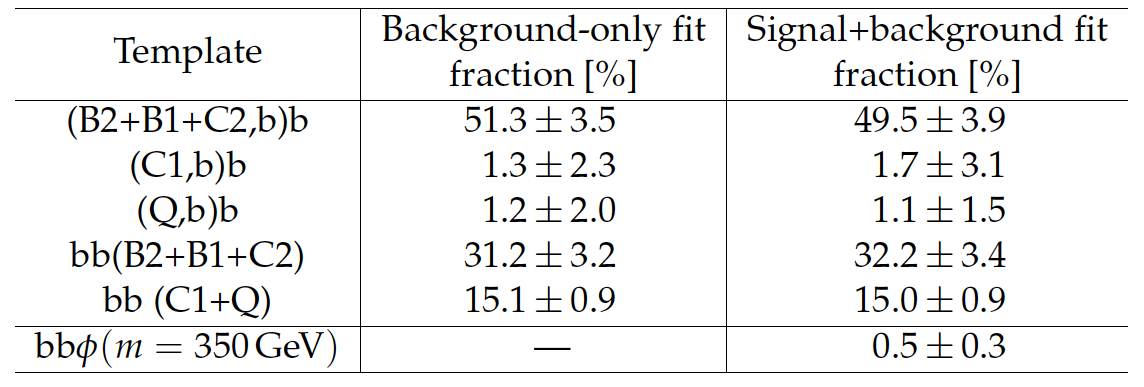
Relative contributions of the individual templates as determined by the background-only and by the signal+background fit for a Higgs boson mass hypothesis of 350 GeV. |

png pdf |
Table 4:
The total signal efficiency in per mille as a function of the Higgs boson mass $ {m_{\phi }} $, for a center-of-mass energy of 8 TeV. |

png pdf |
Table 5:
Expected and observed 95% CL upper limits on $\sigma ( {\mathrm {p}} {\mathrm {p}}\to {\mathrm {b}} \phi +\mathrm {X}) \mathcal {B}(\phi \to { {\mathrm {b}} {\overline {\mathrm {b}}}} )$ in pb as a function of $ {m_{\phi }} $, where $\phi $ denotes a generic Higgs-like state, as obtained from the 8 TeV data. |

png pdf |
Table 6:
Expected and observed 95% CL upper limits on $\tan \beta $ as a function of $ {m_{\mathrm {A}}} $ in the $ {m_{ {\mathrm {h}} }^{\text {max}}} $, $\mu =$ +200 GeV, benchmark scenario obtained from the 8 TeV data only. |

png pdf |
Table 7:
Expected and observed 95% CL upper limits on $\tan \beta $ as a function of $ {m_{\mathrm {A}}} $ in the $ {m_{ {\mathrm {h}} }^{\text {max}}} $, $\mu =$ +200 GeV, benchmark scenario obtained from a combination of the 7 and 8 TeV data. |

png pdf |
Table 8:
Expected and observed 95% CL upper limits on $\tan \beta $ as a function of $ {m_{\mathrm {A}}} $ in the $ {m_{ {\mathrm {h}} }^{\text {mod+}}} $, $\mu =$ +200 GeV, benchmark scenario obtained from a combination of the 7 and 8 TeV data. |

png pdf |
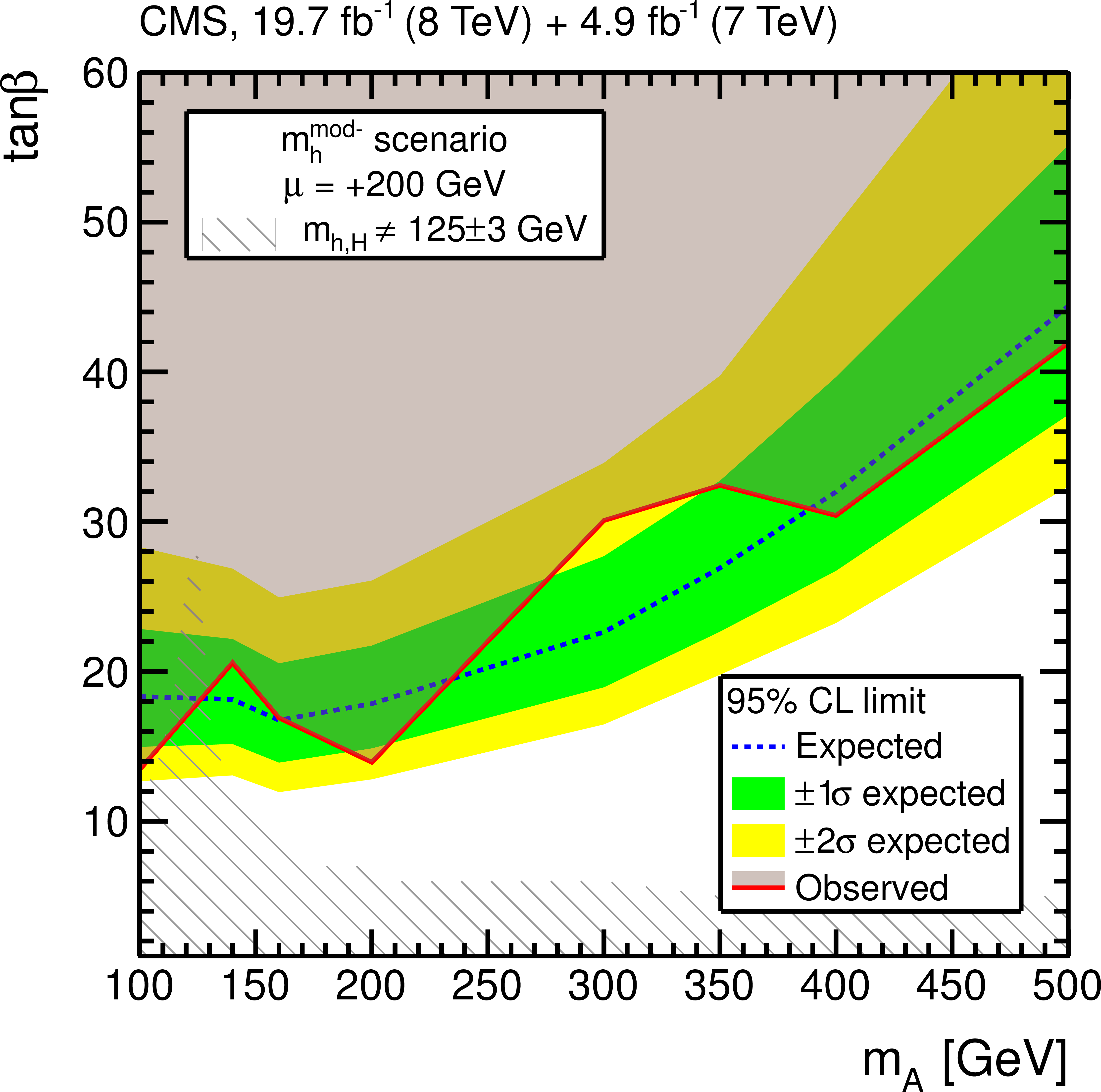
Table 9:
Expected and observed 95% CL upper limits on $\tan \beta $ as a function of $ {m_{\mathrm {A}}} $ in the $ {m_{ {\mathrm {h}} }^{\text {mod-}}} $, $\mu = $ +200 GeV, benchmark scenario obtained from a combination of the 7 and 8 TeV data. |

png pdf |
Table 10:
Expected and observed 95% CL upper limits on $\tan \beta $ as a function of $ {m_{\mathrm {A}}} $ in the light-stau, $\mu =$ +200 GeV, benchmark scenario obtained from a combination of the 7 and 8 TeV data. |

png pdf |
Table 11:
Expected and observed 95% CL upper limits on $\tan \beta $ as a function of $ {m_{\mathrm {A}}} $ in the light-stop, $\mu =$ +200 GeV, benchmark scenario obtained from a combination of the 7 and 8 TeV data. |

png pdf |
Table 12:
Observed (expected) 95% CL upper limits on $\tan \beta $ as a function of $ {m_{\mathrm {A}}} $ in the $ {m_{ {\mathrm {h}} }^{\text {mod+}}} $ benchmark scenario for different values of the higgsino mass parameter $\mu $ obtained from a combination of the 7 and 8 TeV data. |
| Summary |
| A search for a Higgs boson decaying into a pair of b quarks and accompanied by at least one additional b quark has been performed in proton-proton collisions at a center-of-mass energy of 8 TeV at the LHC, corresponding to an integrated luminosity of 19.7 fb$^{-1}$. The data were taken with dedicated triggers using all-hadronic jet signatures combined with online b tagging. A selection of events with three b-tagged jets has been performed in the offline analysis. A signal has been searched for in the two-dimensional spectrum formed by the invariant mass of the two leading jets and a condensed event b-tag estimator. No evidence for a signal is found. The observed distributions are well described by a background model constructed from events in which only two of the three leading jets are required to be b tagged. Upper limits on the Higgs boson cross section times branching fraction are obtained in the mass region from 100 to 900 GeV, thus extending the search to considerably higher masses than those accessed by the previous 7 TeV analysis. The upper limits range from about 250 pb at the lower end of the mass range, to about 1 pb at 900 GeV. The results are interpreted within the MSSM in the benchmark scenarios $m_{\mathrm{h}}^{\mathrm{max}}$, $m_{\mathrm{h}}^{\mathrm{mod+}}$, $m_{\mathrm{h}}^{\mathrm{mod-}}$, light-stau and light-stop, and lead to upper limits for the model parameter $\tan \beta$ as a function of the mass parameter $m_{\mathrm{A}}$. In combination with the 7 TeV data, the observed limit for $\tan \beta$ ranges down to about 14 at the lowest $m_{\mathrm{A}}$ value of 100 GeV in the $m_{\mathrm{h}}^{\mathrm{mod+}}$ scenario with a higgsino mass parameter of $\mu =$ +200 GeV. The limit depends significantly on $\mu$, varying from $\tan \beta =$ 30 for $\mu = -$500 GeV to beyond 60 for $\mu =$ +500 GeV at $m_{\mathrm{A}} =$ 500 GeV. |
| Additional Figures | |

png pdf |
Additional Figure 1:
Distribution of the sum of secondary-vertex masses of CSVT b-tagged jets for different jet flavours. |

png pdf |
Additional Figure 2:
$M_{12}$ projections of the five background templates used in the fit (on a logarithmic scale). |

png pdf |
Additional Figure 3:
Unrolled slices of the 2D distributions in ($M_{12}$,$X_{123}$) space after the background-only fit. The $M_{12}$ slices for all nine values of $X_{123}$ are shown in concatenation. In this case the bin contents are not normalized to the bin size. For this reason, a ``step'' is visible in the falling slope of the $M_{12}$ distribution at $M_{12}$=300\,GeV, where the bin size changes. The hatched band shows the background histogram uncertainty, which results from the pre-fit bin-by-bin statistical and systematic errors. The shaded band shows the full post-fit uncertainty, which includes also uncertainties beyond the bin-by-bin level, i.e. from nuisance parameters whose impact may be correlated across the bins. |

png pdf |
Additional Figure 4:
Projection of the dijet mass $M_{12}$ in the triple-b-tag sample, together with the corresponding projections of the fitted background templates on a logarithmic scale. The hatched area at the end of the summed background histogram shows the bin-by-bin background uncertainty propagated from the templates. In addition, the ratio to the background estimate is shown at the bottom. |

png pdf |
Additional Figure 5:
Unrolled slices of the 2D distributions in ($M_{12}$,$X_{123}$) space after the combined fit of signal and background templates for the 350 GeV mass point. The $M_{12}$ slices for all nine values of $X_{123}$ are shown in concatenation. In this case the bin contents are not normalized to the bin size. For this reason, a ``step'' is visible in the falling slope of the $M_{12}$ distribution at $M_{12}$=300\,GeV, where the bin size changes. The hatched band shows the background histogram uncertainty, which results from the pre-fit bin-by-bin statistical and systematic errors. The shaded band shows the full post-fit uncertainty, which includes also uncertainties beyond the bin-by-bin level, i.e. from nuisance parameters whose impact may be correlated across the bins. |
png pdf |
Additional Figure 6:
Results from the combined fit of signal and background templates in the triple-b-tag sample, at the 350 GeV mass point. The plot shows the projection of the dijet mass $M_{12}$ on a logarithmic scale. The hatched area at the end of the summed background histogram shows the pre-fit bin-by-bin background uncertainty propagated from the templates. In addition, the ratio to the background estimate is shown at the bottom. |

png pdf |
Additional Figure 7:
As Fig. 5 (aux), but the ratio to the sum of signal and background prediction is shown. |

png pdf |
Additional Figure 8:
As Fig. 6 (aux), but the ratio to the sum of signal and background prediction is shown. |

png pdf |
Additional Figure 9:
As Fig. 8 (aux), but on a logarithmic scale. |

png pdf |
Additional Figure 10:
As Fig. 6 (aux), but the projection of the $X_{123}$ variable is shown. |

png pdf |
Additional Figure 11:
Comparison of the expected and observed upper limits at 95% CL for the MSSM parameter $\tan\beta$ versus $m_{\rm A}$ in the $m^{\rm mod+}_{\rm h}$ benchmark scenario obtained in different final states: $\phi \rightarrow\mathrm{bb}$ (this analysis), $\phi\rightarrow\mu\mu$ (CMS-HIG-13-024, submitted to Phys. Lett. B), and $\phi\rightarrow\tau\tau$ (CMS-HIG-14-029). The shaded areas mark the excluded regions. |
|
|
Compact Muon Solenoid LHC, CERN |
|

|

|

|

|

|