CMS-HIG-14-034

CMS-HIG-14-034 ; CERN-PH-EP-2015-211
Searches for a heavy scalar boson $\mathrm{H}$ decaying to a pair of 125 GeV Higgs bosons $ \mathrm{hh} $ or for a heavy pseudoscalar boson $ \mathrm{A} $ decaying to $ \mathrm{Zh} $, in the final states with $\mathrm{h} \to \tau \tau$
CMS Collaboration
5 October 2015
Phys. Lett. B 755 (2016) 217
Abstract: A search for a heavy scalar boson $ \mathrm{H} $ decaying into a pair of lighter standard-model-like 125 GeV Higgs bosons $ \mathrm{h} $ and a search for a heavy pseudoscalar boson $ \mathrm{A} $ decaying into a $ \mathrm{Z}$ and an $ \mathrm{h} $ boson are presented. The searches are performed on a dataset corresponding to an integrated luminosity of 19.7 fb$^{-1}$ of pp collision data at a centre-of-mass energy of 8 TeV, collected by CMS in 2012. A final state consisting of two $\tau$ leptons and two b jets is used to search for the $\mathrm{ H \to h h }$ decay. A final state consisting of two $\tau$ leptons from the $ \mathrm{h} $ boson decay, and two additional leptons from the $ \mathrm{Z}$ boson decay, is used to search for the decay $\mathrm{ A \to Z h } $. The results are interpreted in the context of both the minimal supersymmetric extension of the standard model and two-Higgs-doublet models. No excess is found above the standard model expectation and upper limits are set on the heavy boson production cross sections in the mass ranges 260 $ < m_{\mathrm{H}} < $ 350 GeV and 220 $ < m_{\mathrm{A} } < $ 350 GeV.
Links: e-print arXiv:1510.01181 [hep-ex] (PDF) ; CDS record ; inSPIRE record ; CADI line (restricted) ;

Figures	Summary	Additional Figures	CMS Publications

Figures
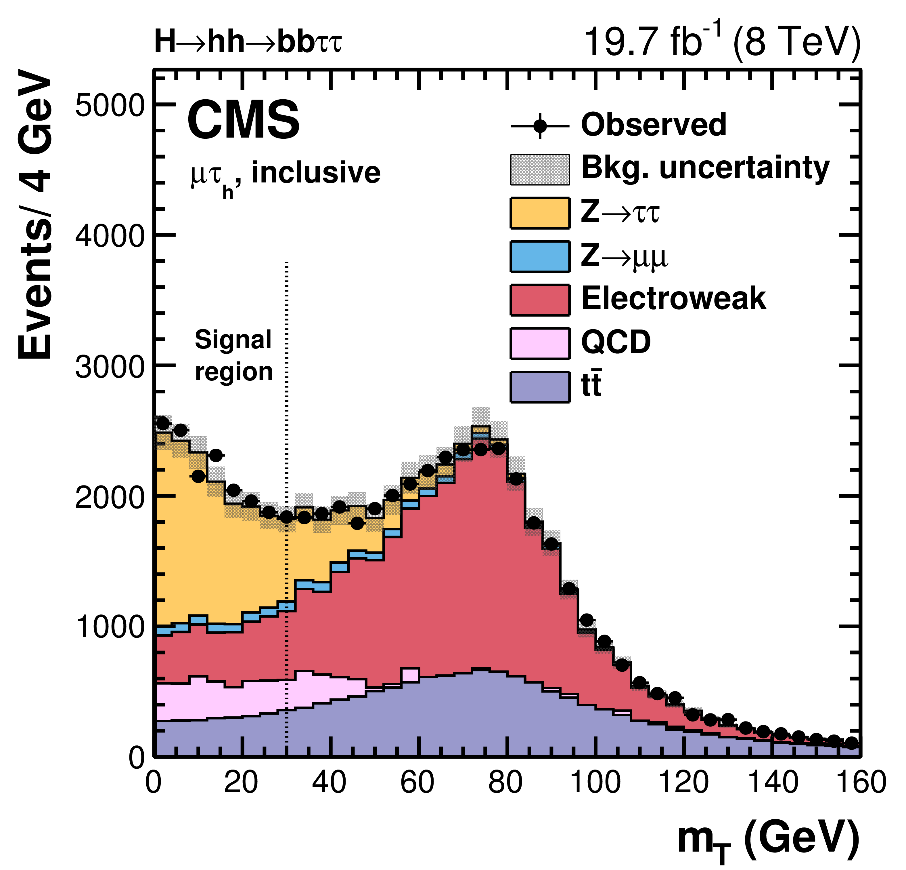
png pdf	Figure 1: Distribution of $ {m_\mathrm {T}} $ for events in the $\mu {\tau _\mathrm{h} } $ final state, containing at least two additional jets. The $\mathrm{W} $+jets background is included in the ``electroweak" category. Multijet events are indicated as QCD. The $\mathrm{h} \to \mathrm{h} \mathrm{h} \to \mathrm{b} \mathrm{b} \tau \tau $ selection requires $ {m_\mathrm {T}} <$ 30 GeV for the $\mu {\tau _\mathrm{h} } $ and $\mathrm{e} {\tau _\mathrm{h} } $ final states.
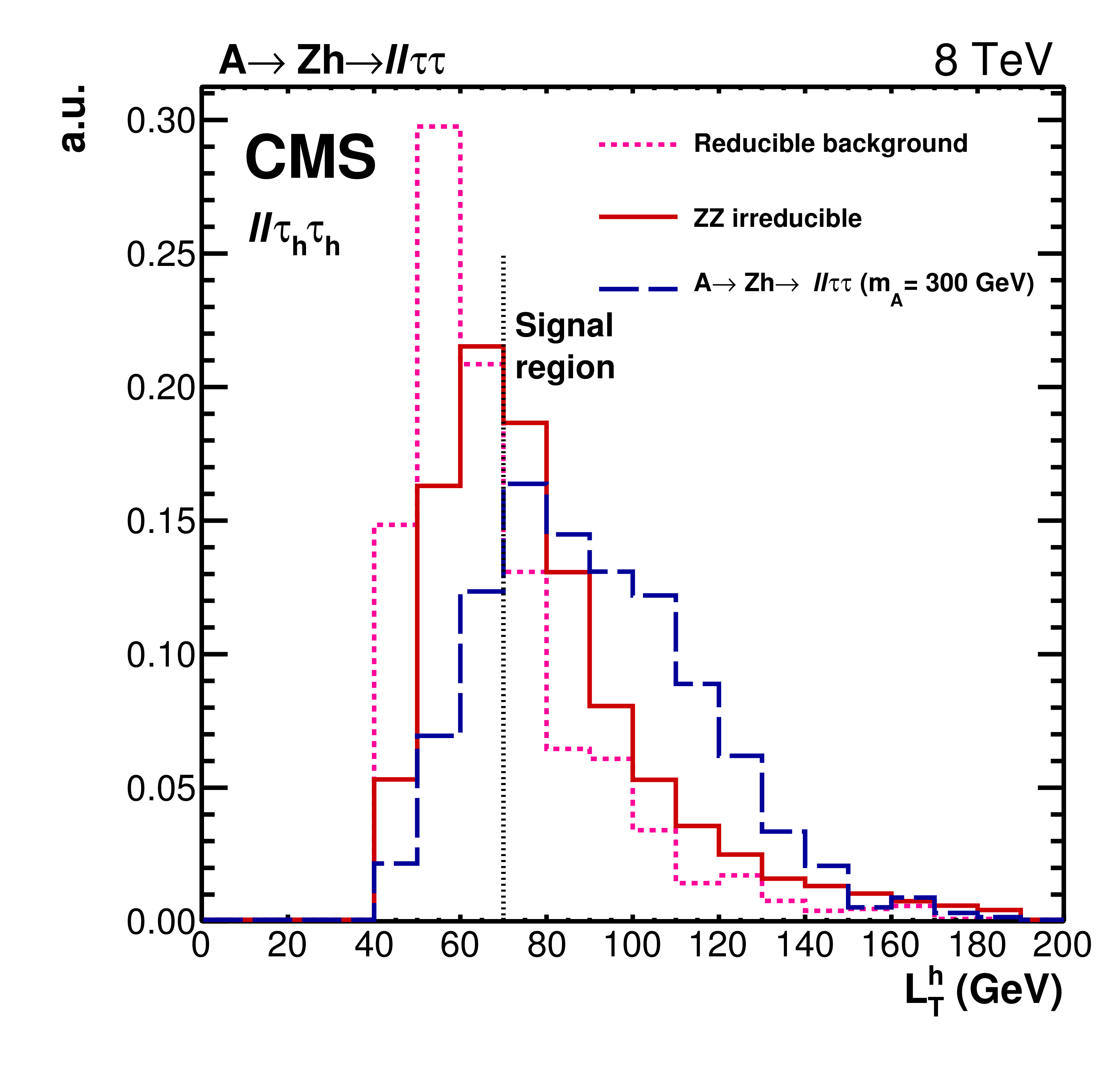
png pdf	Figure 2: Distribution of the variable $L_\mathrm {T}^{\mathrm{h} }$ for events in the ${\ell \ell } {\tau _\mathrm{h} } {\tau _\mathrm{h} } $ final state. The reducible background is estimated from data, instead the ZZ irreducible background from simulation.
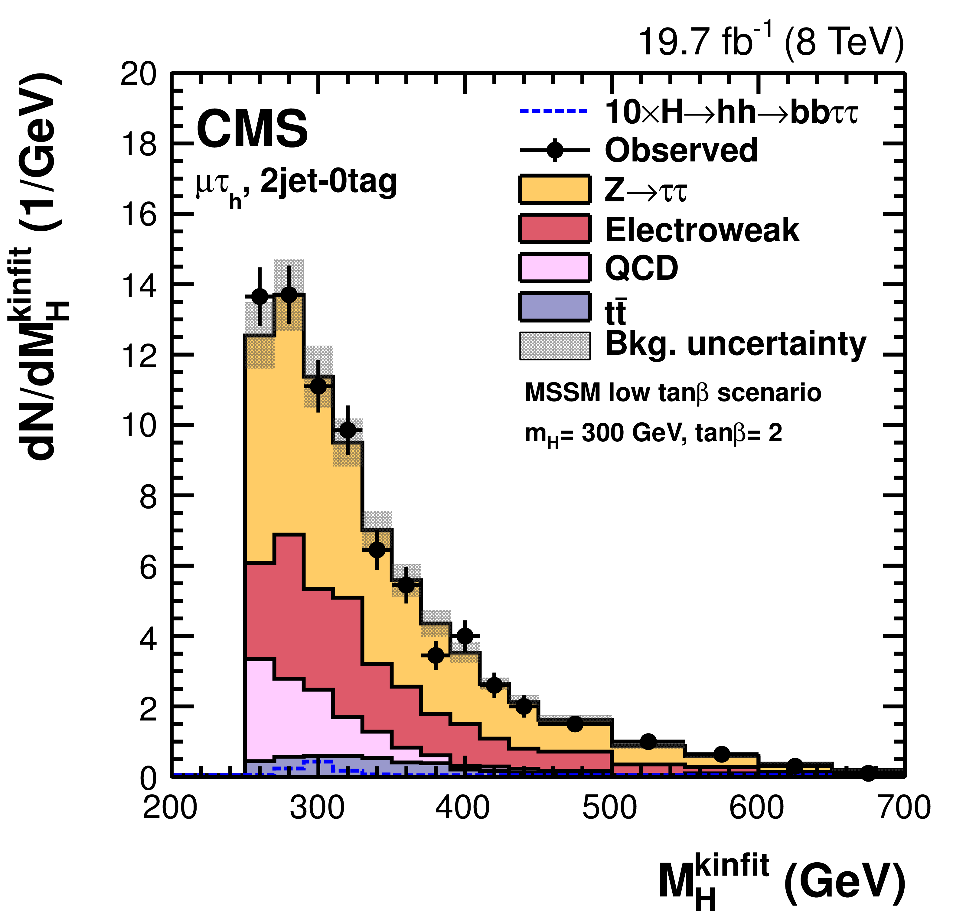
png pdf	Figure 3-a: Distributions of the reconstructed four-body mass with the kinematic fit after applying mass selections on $m_{\tau \tau }$ and $m_{\mathrm{b} \mathrm{b} }$ in the $\mu {\tau _\mathrm{h} } $ channel. The plots are shown for events in the 2jet--0tag (a), 2jet--1tag (b), and 2jet--2tag (c) categories. The expected signal scaled by a factor 10 is shown superimposed as an open dashed histogram for $\tan\beta =$ 2 and $m_{\mathrm{h} }=$ 300 GeV in the low $\tan\beta $ scenario of the MSSM. Expected background contributions are shown for the values of nuisance parameters (systematic uncertainties) obtained after fitting the signal plus background hypothesis to the data.
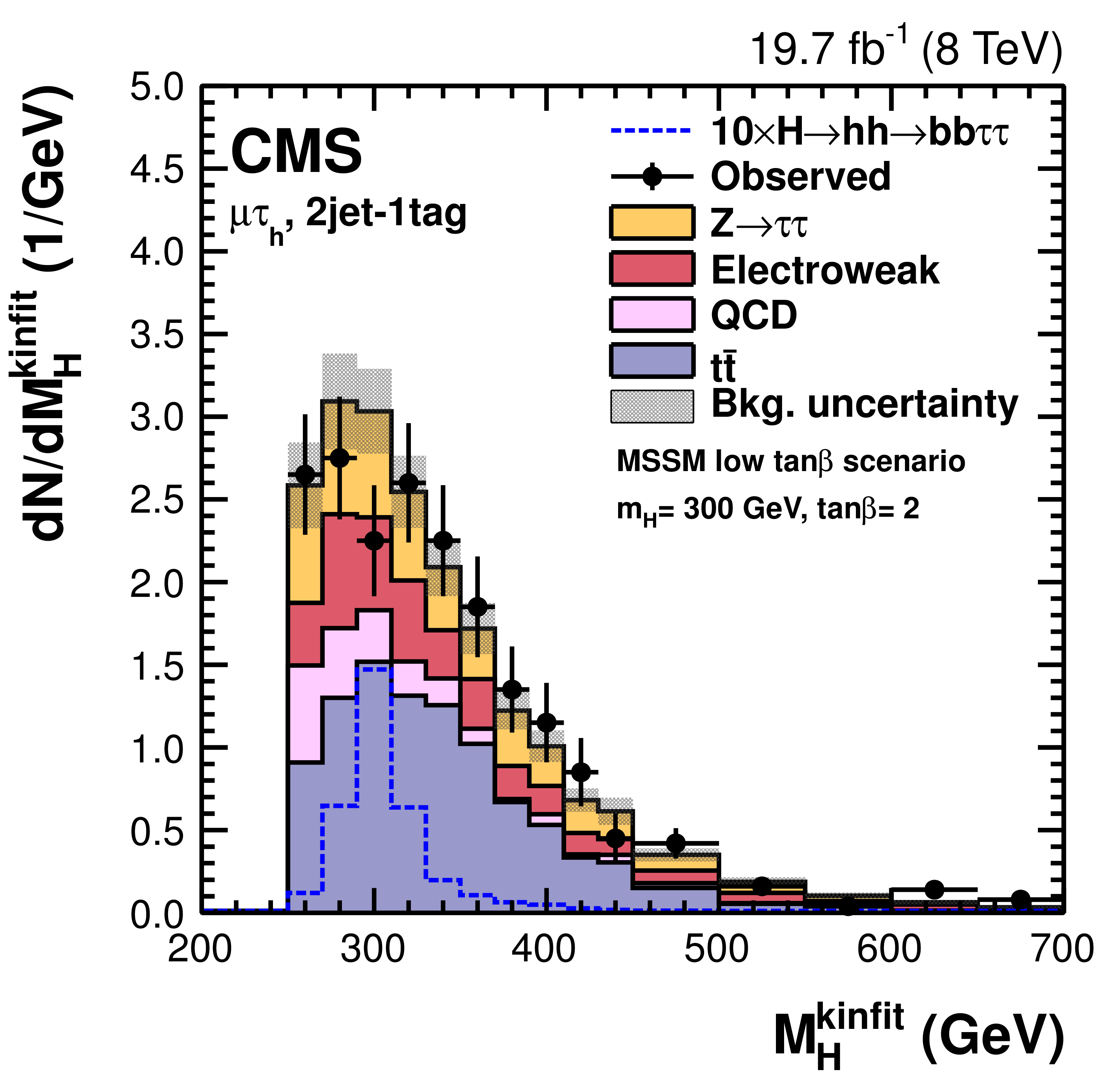
png pdf	Figure 3-b: Distributions of the reconstructed four-body mass with the kinematic fit after applying mass selections on $m_{\tau \tau }$ and $m_{\mathrm{b} \mathrm{b} }$ in the $\mu {\tau _\mathrm{h} } $ channel. The plots are shown for events in the 2jet--0tag (a), 2jet--1tag (b), and 2jet--2tag (c) categories. The expected signal scaled by a factor 10 is shown superimposed as an open dashed histogram for $\tan\beta =$ 2 and $m_{\mathrm{h} }=$ 300 GeV in the low $\tan\beta $ scenario of the MSSM. Expected background contributions are shown for the values of nuisance parameters (systematic uncertainties) obtained after fitting the signal plus background hypothesis to the data.
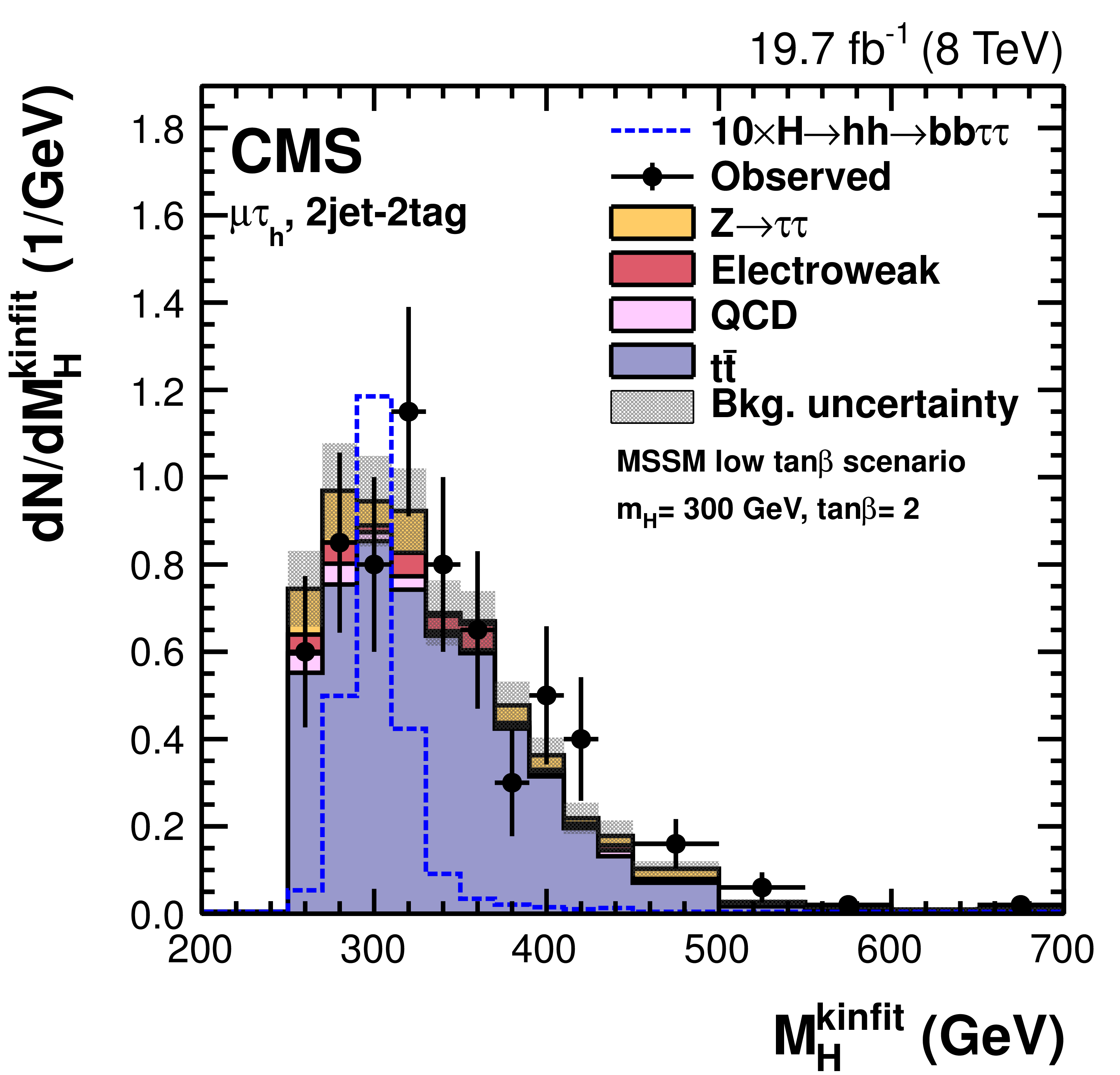
png pdf	Figure 3-c: Distributions of the reconstructed four-body mass with the kinematic fit after applying mass selections on $m_{\tau \tau }$ and $m_{\mathrm{b} \mathrm{b} }$ in the $\mu {\tau _\mathrm{h} } $ channel. The plots are shown for events in the 2jet--0tag (a), 2jet--1tag (b), and 2jet--2tag (c) categories. The expected signal scaled by a factor 10 is shown superimposed as an open dashed histogram for $\tan\beta =$ 2 and $m_{\mathrm{h} }=$ 300 GeV in the low $\tan\beta $ scenario of the MSSM. Expected background contributions are shown for the values of nuisance parameters (systematic uncertainties) obtained after fitting the signal plus background hypothesis to the data.
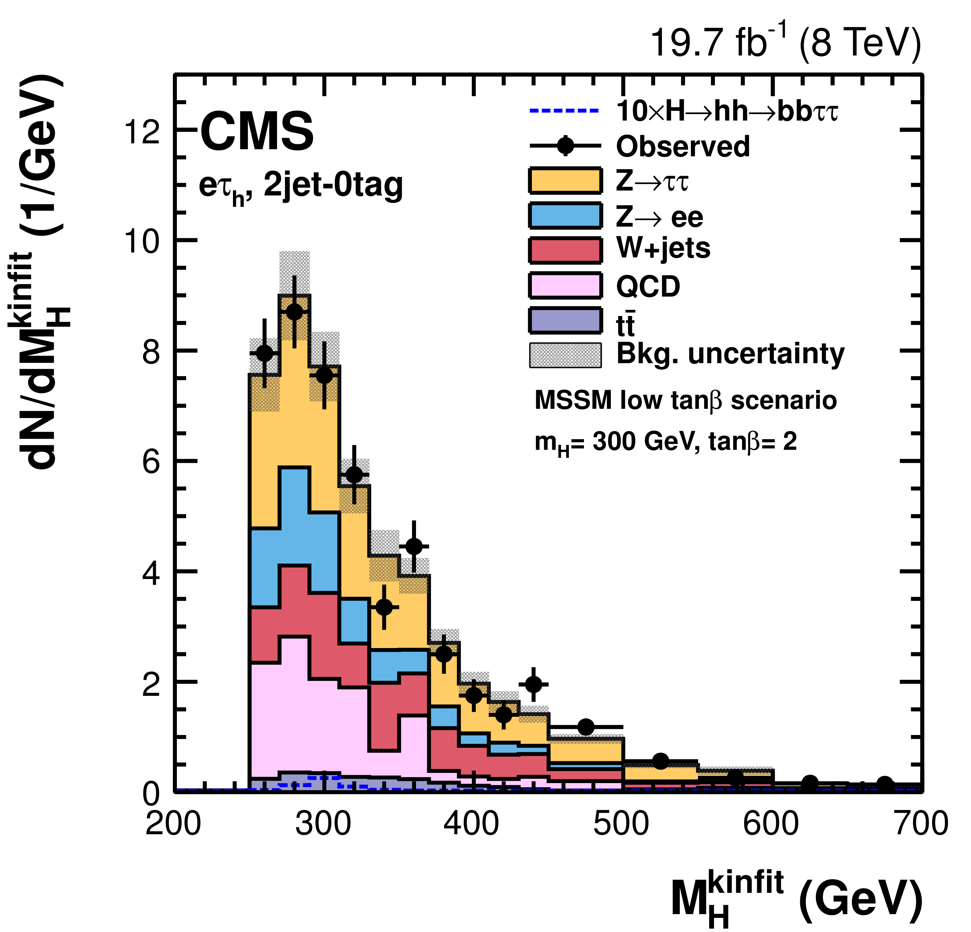
png pdf	Figure 4-a: Distributions of the reconstructed four-body mass with the kinematic fit after applying mass selections on $m_{\tau \tau }$ and $m_{\mathrm{b} \mathrm{b} }$ in the $\mathrm{e} {\tau _\mathrm{h} } $ channel. The plots are shown for events in the 2jet--0tag (a), 2jet--1tag (b), and 2jet--2tag (c) categories. The expected signal scaled by a factor 10 is shown superimposed as an open dashed histogram for $\tan\beta =$ 2 and $m_{\mathrm{h} }=$ 300 GeV in the low $\tan\beta $ scenario of the MSSM. Expected background contributions are shown for the values of nuisance parameters (systematic uncertainties) obtained after fitting the signal plus background hypothesis to the data.
png pdf	Figure 4-b: Distributions of the reconstructed four-body mass with the kinematic fit after applying mass selections on $m_{\tau \tau }$ and $m_{\mathrm{b} \mathrm{b} }$ in the $\mathrm{e} {\tau _\mathrm{h} } $ channel. The plots are shown for events in the 2jet--0tag (a), 2jet--1tag (b), and 2jet--2tag (c) categories. The expected signal scaled by a factor 10 is shown superimposed as an open dashed histogram for $\tan\beta =$ 2 and $m_{\mathrm{h} }=$ 300 GeV in the low $\tan\beta $ scenario of the MSSM. Expected background contributions are shown for the values of nuisance parameters (systematic uncertainties) obtained after fitting the signal plus background hypothesis to the data.
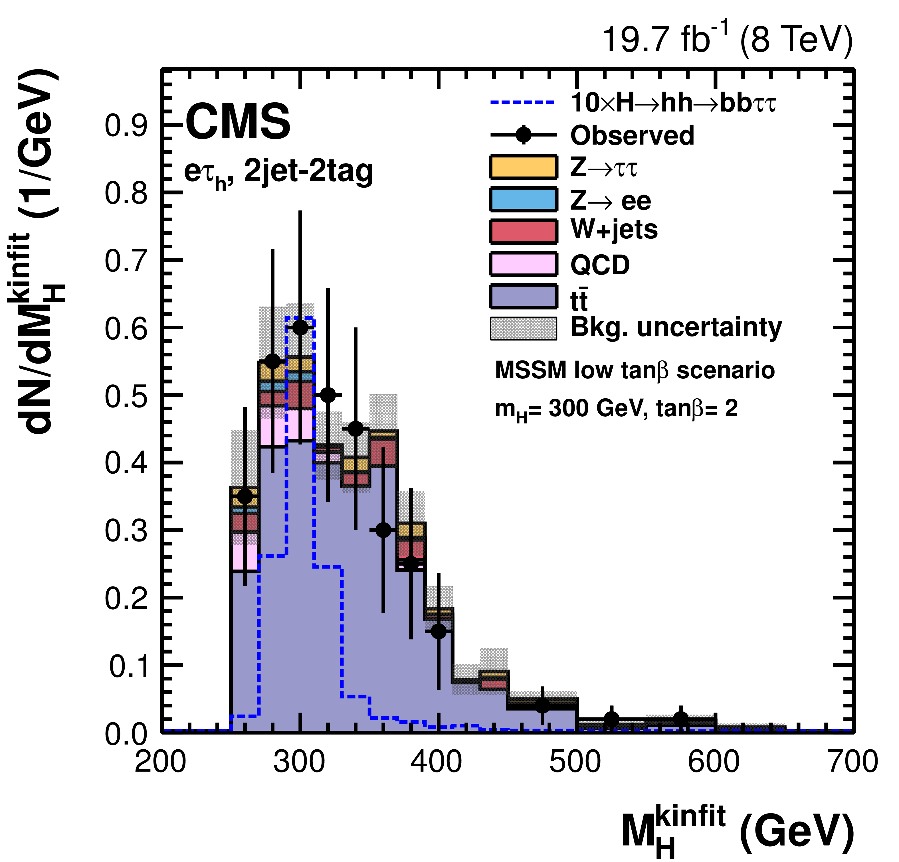
png pdf	Figure 4-c: Distributions of the reconstructed four-body mass with the kinematic fit after applying mass selections on $m_{\tau \tau }$ and $m_{\mathrm{b} \mathrm{b} }$ in the $\mathrm{e} {\tau _\mathrm{h} } $ channel. The plots are shown for events in the 2jet--0tag (a), 2jet--1tag (b), and 2jet--2tag (c) categories. The expected signal scaled by a factor 10 is shown superimposed as an open dashed histogram for $\tan\beta =$ 2 and $m_{\mathrm{h} }=$ 300 GeV in the low $\tan\beta $ scenario of the MSSM. Expected background contributions are shown for the values of nuisance parameters (systematic uncertainties) obtained after fitting the signal plus background hypothesis to the data.
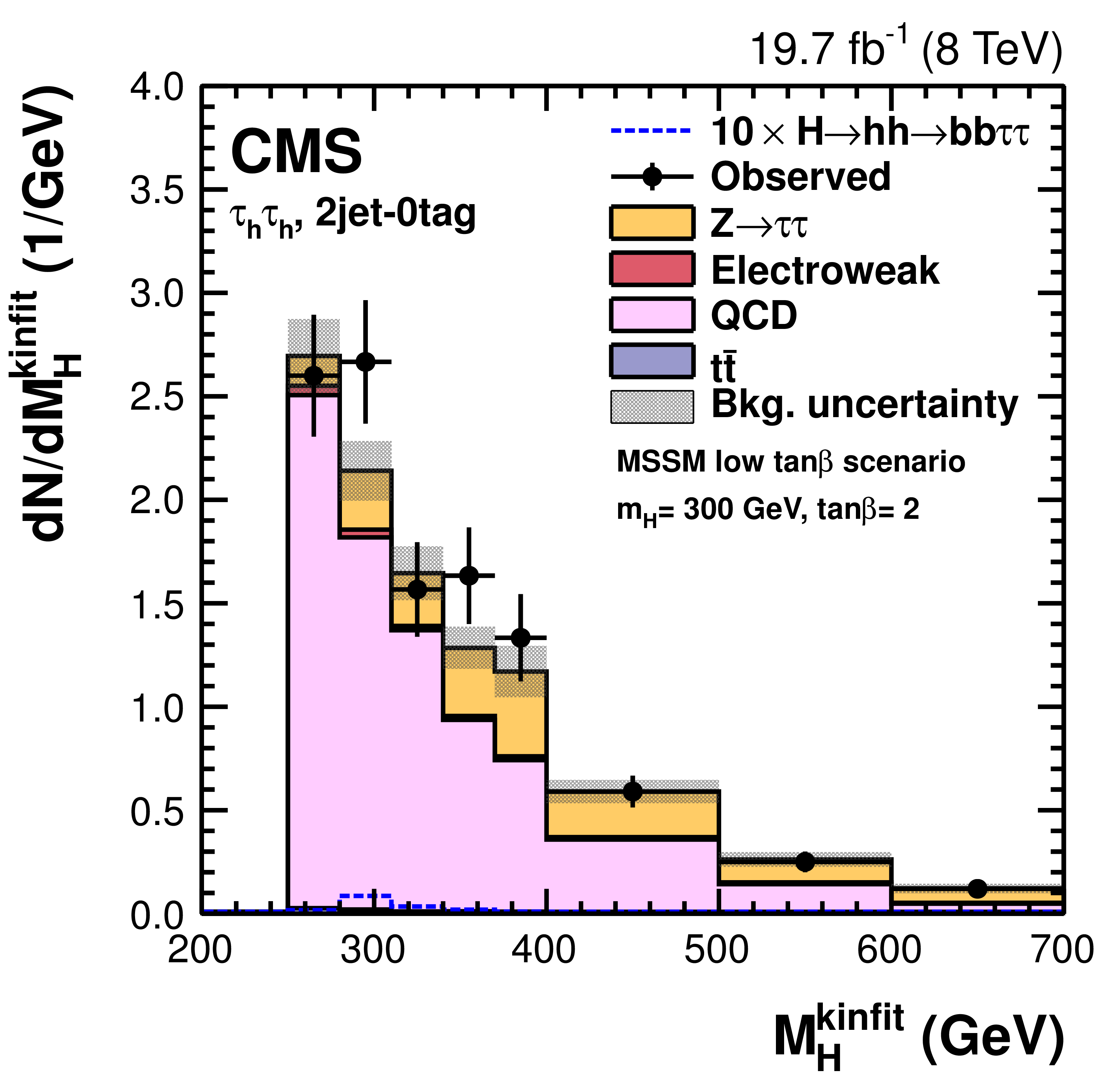
png pdf	Figure 5-a: Distributions of the reconstructed four-body mass with the kinematic fit after applying mass selections on $m_{\tau \tau }$ and $m_{\mathrm{b} \mathrm{b} }$ in the $ {\tau _\mathrm{h} } {\tau _\mathrm{h} } $ channel. The plots are shown for events in the 2jet--0tag (a), 2jet--1tag (b), and 2jet--2tag (c) categories. The expected signal scaled by a factor 10 is shown superimposed as an open dashed histogram for $\tan\beta =$ 2 and $m_{\mathrm{h} }=$ 300 GeV in the low $\tan\beta $ scenario of the MSSM. Expected background contributions are shown for the values of nuisance parameters (systematic uncertainties) obtained after fitting the signal plus background hypothesis to the data.
png pdf	Figure 5-b: Distributions of the reconstructed four-body mass with the kinematic fit after applying mass selections on $m_{\tau \tau }$ and $m_{\mathrm{b} \mathrm{b} }$ in the $ {\tau _\mathrm{h} } {\tau _\mathrm{h} } $ channel. The plots are shown for events in the 2jet--0tag (a), 2jet--1tag (b), and 2jet--2tag (c) categories. The expected signal scaled by a factor 10 is shown superimposed as an open dashed histogram for $\tan\beta =$ 2 and $m_{\mathrm{h} }=$ 300 GeV in the low $\tan\beta $ scenario of the MSSM. Expected background contributions are shown for the values of nuisance parameters (systematic uncertainties) obtained after fitting the signal plus background hypothesis to the data.
png pdf	Figure 5-c: Distributions of the reconstructed four-body mass with the kinematic fit after applying mass selections on $m_{\tau \tau }$ and $m_{\mathrm{b} \mathrm{b} }$ in the $ {\tau _\mathrm{h} } {\tau _\mathrm{h} } $ channel. The plots are shown for events in the 2jet--0tag (a), 2jet--1tag (b), and 2jet--2tag (c) categories. The expected signal scaled by a factor 10 is shown superimposed as an open dashed histogram for $\tan\beta =$ 2 and $m_{\mathrm{h} }=$ 300 GeV in the low $\tan\beta $ scenario of the MSSM. Expected background contributions are shown for the values of nuisance parameters (systematic uncertainties) obtained after fitting the signal plus background hypothesis to the data.
png pdf	Figure 6-a: Invariant mass distributions for different final states of the $ {\mathrm {A}} \to \mathrm{Z} \mathrm{h} $ process where $\mathrm{Z} $ decays to $\mathrm{e} \mathrm{e} $. The expected signal scaled by a factor 5 is shown superimposed as an open dashed histogram for $\tan\beta =$ 2 and $m_{ {\mathrm {A}} }=$ 300 GeV in the low $\tan\beta $ scenario of MSSM. Expected background contributions are shown for the values of nuisance parameters (systematic uncertainties) obtained after fitting the signal plus background hypothesis to the data.
png pdf	Figure 6-b: Invariant mass distributions for different final states of the $ {\mathrm {A}} \to \mathrm{Z} \mathrm{h} $ process where $\mathrm{Z} $ decays to $\mathrm{e} \mathrm{e} $. The expected signal scaled by a factor 5 is shown superimposed as an open dashed histogram for $\tan\beta =$ 2 and $m_{ {\mathrm {A}} }=$ 300 GeV in the low $\tan\beta $ scenario of MSSM. Expected background contributions are shown for the values of nuisance parameters (systematic uncertainties) obtained after fitting the signal plus background hypothesis to the data.
png pdf	Figure 6-c: Invariant mass distributions for different final states of the $ {\mathrm {A}} \to \mathrm{Z} \mathrm{h} $ process where $\mathrm{Z} $ decays to $\mathrm{e} \mathrm{e} $. The expected signal scaled by a factor 5 is shown superimposed as an open dashed histogram for $\tan\beta =$ 2 and $m_{ {\mathrm {A}} }=$ 300 GeV in the low $\tan\beta $ scenario of MSSM. Expected background contributions are shown for the values of nuisance parameters (systematic uncertainties) obtained after fitting the signal plus background hypothesis to the data.
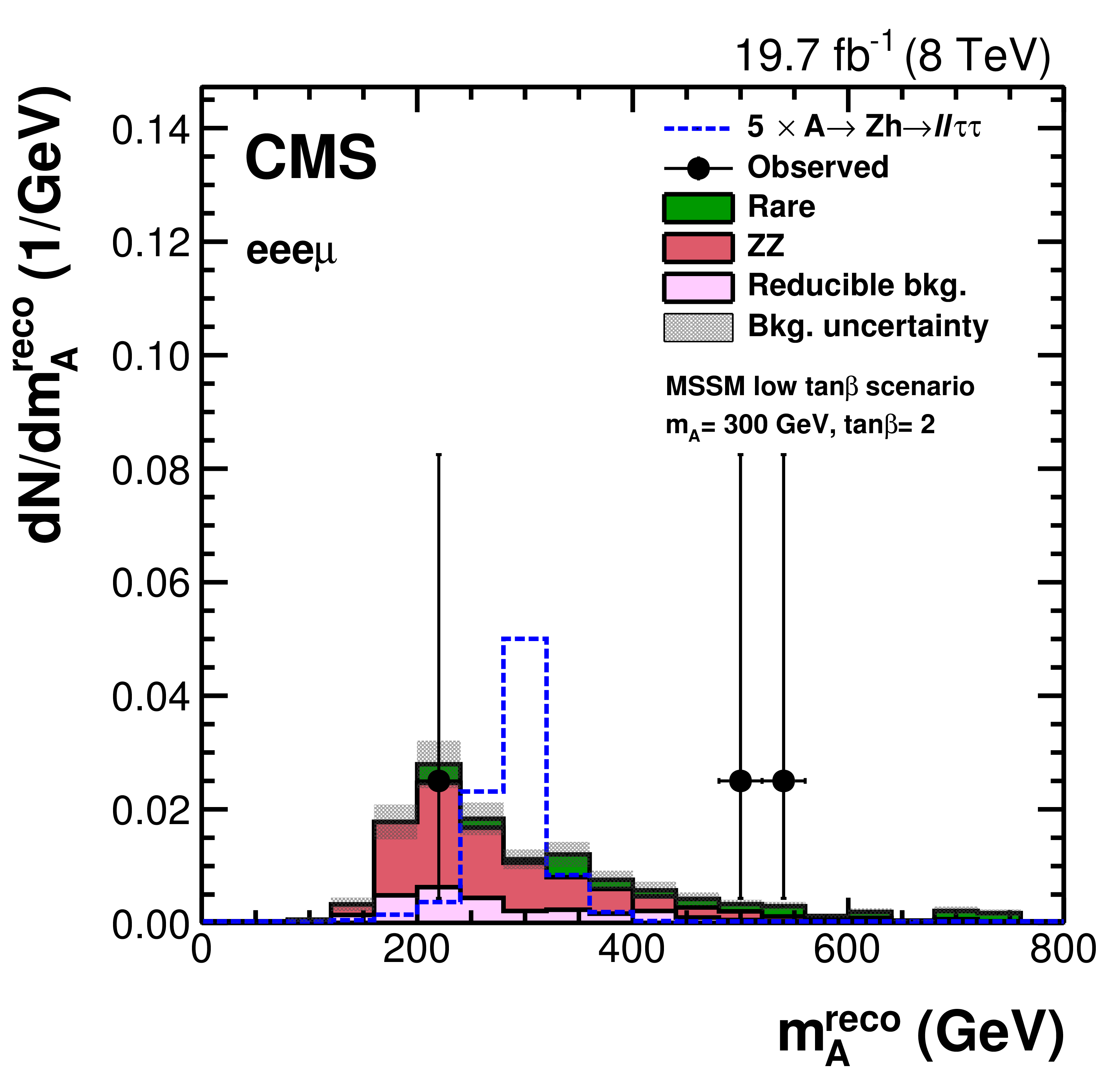
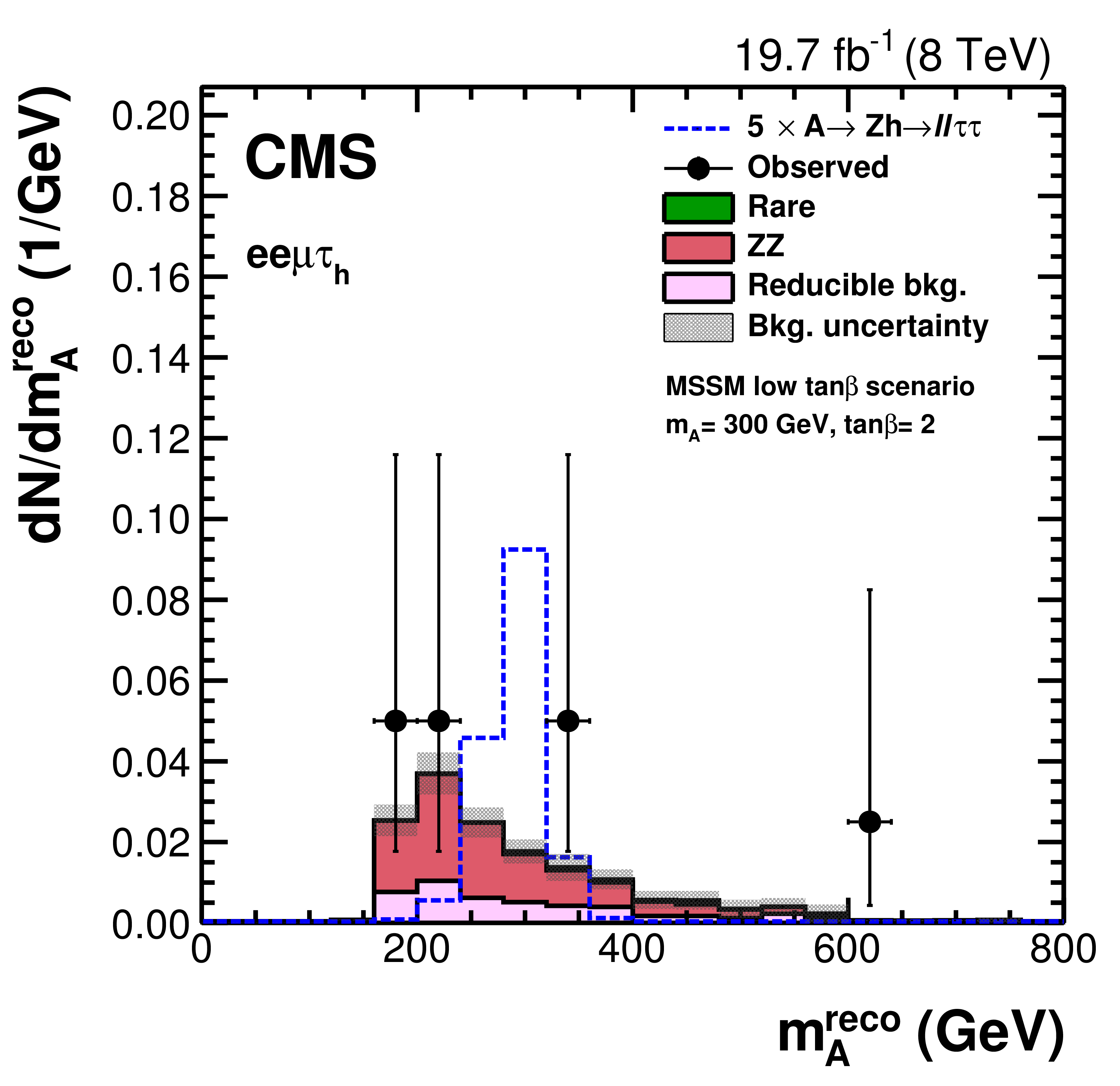
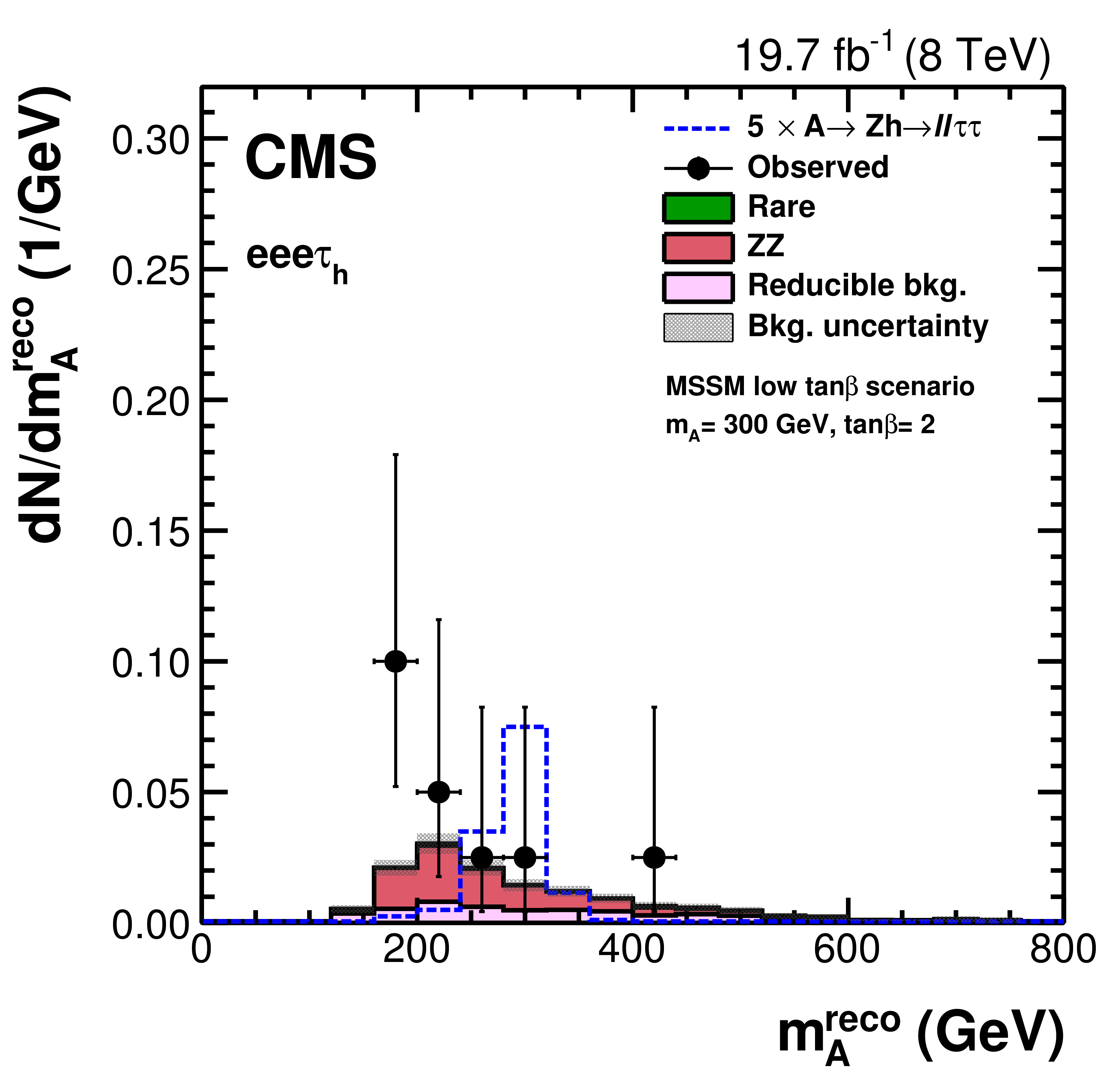
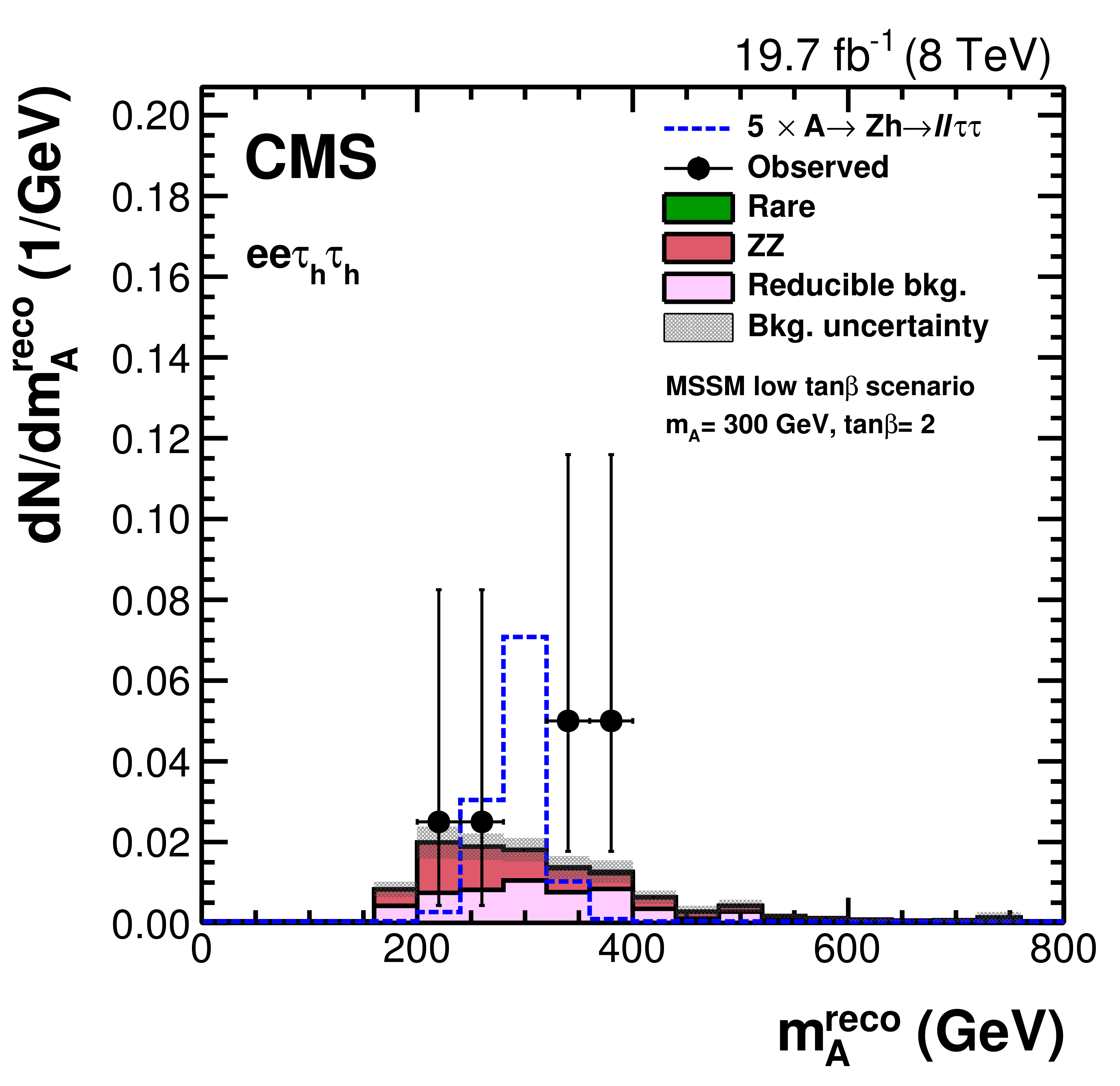
png pdf	Figure 6-d: Invariant mass distributions for different final states of the $ {\mathrm {A}} \to \mathrm{Z} \mathrm{h} $ process where $\mathrm{Z} $ decays to $\mathrm{e} \mathrm{e} $. The expected signal scaled by a factor 5 is shown superimposed as an open dashed histogram for $\tan\beta =$ 2 and $m_{ {\mathrm {A}} }=$ 300 GeV in the low $\tan\beta $ scenario of MSSM. Expected background contributions are shown for the values of nuisance parameters (systematic uncertainties) obtained after fitting the signal plus background hypothesis to the data.
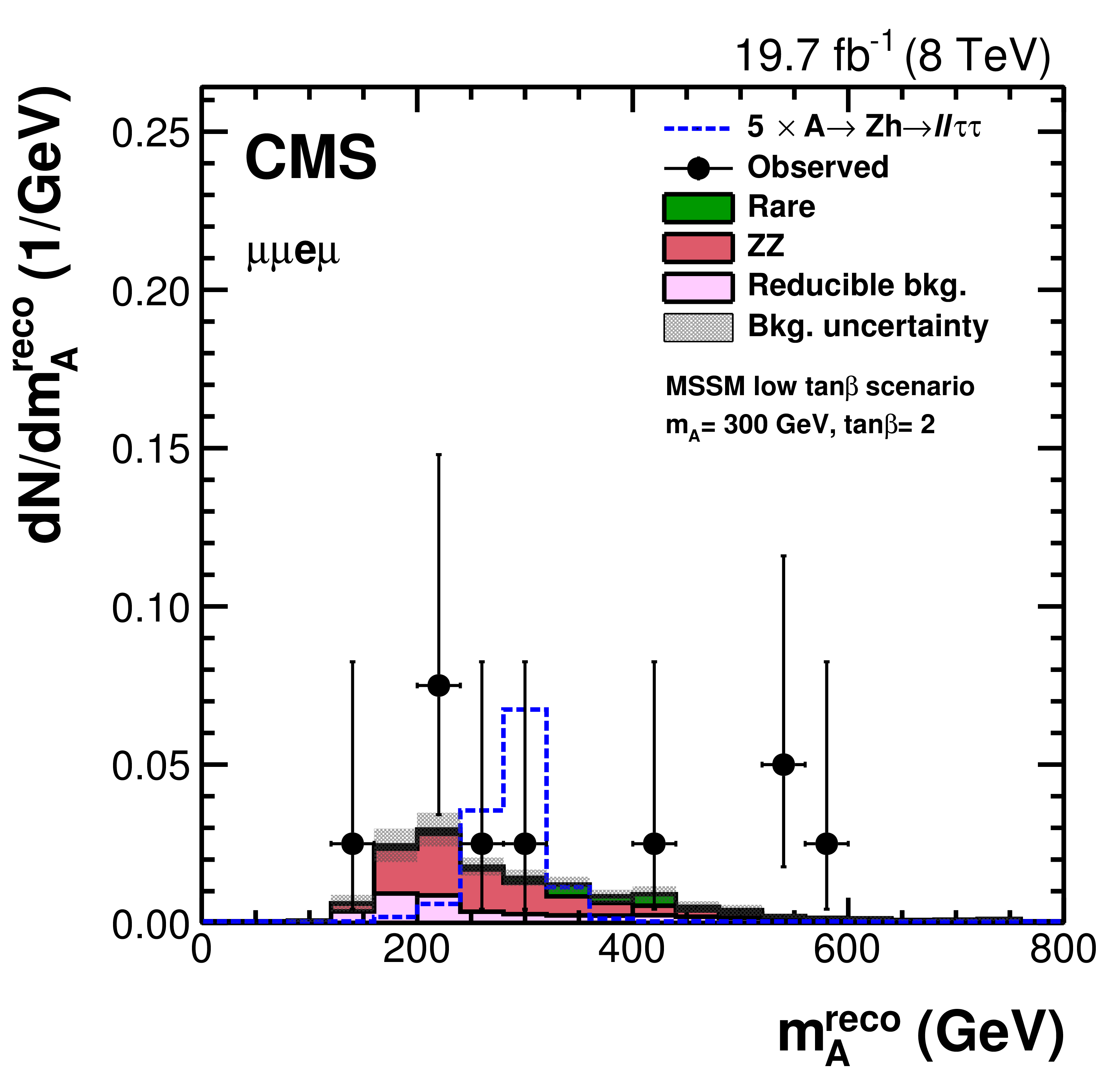
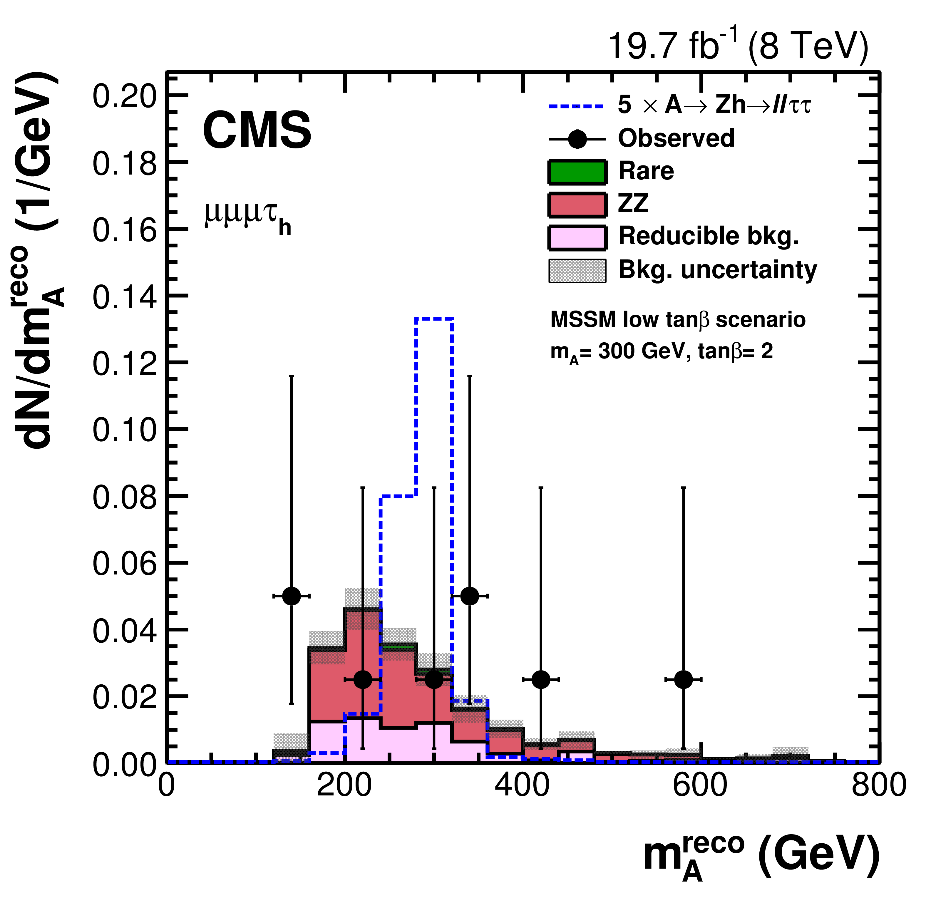
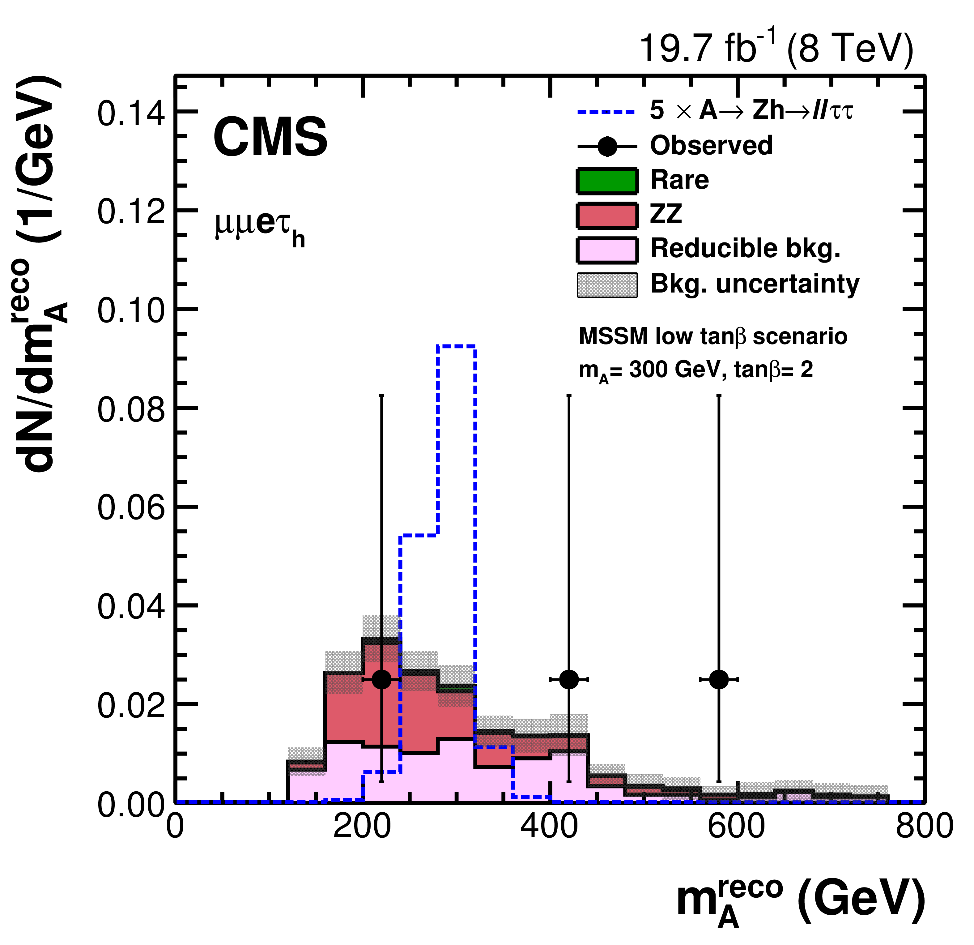
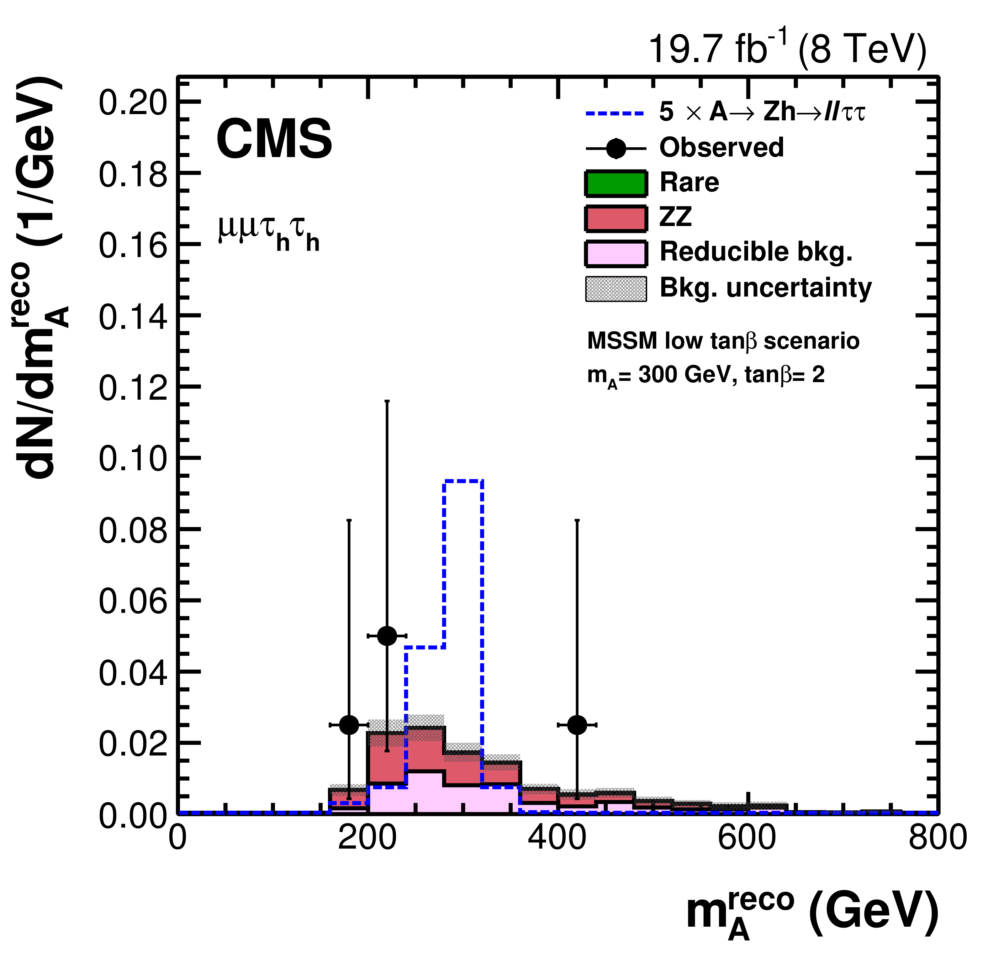
png pdf	Figure 7-a: Invariant mass distributions for different final states of the $ {\mathrm {A}} \to \mathrm{Z} \mathrm{h} $ process where $\mathrm{Z} $ decays to $\mu \mu $. The expected signal scaled by a factor 5 is shown superimposed as an open dashed histogram for $\tan\beta =$ 2 and $m_{ {\mathrm {A}} }=$ 300 GeV in the low $\tan\beta $ scenario of MSSM. Expected background contributions are shown for the values of nuisance parameters (systematic uncertainties) obtained after fitting the signal plus background hypothesis to the data.
png pdf	Figure 7-b: Invariant mass distributions for different final states of the $ {\mathrm {A}} \to \mathrm{Z} \mathrm{h} $ process where $\mathrm{Z} $ decays to $\mu \mu $. The expected signal scaled by a factor 5 is shown superimposed as an open dashed histogram for $\tan\beta =$ 2 and $m_{ {\mathrm {A}} }=$ 300 GeV in the low $\tan\beta $ scenario of MSSM. Expected background contributions are shown for the values of nuisance parameters (systematic uncertainties) obtained after fitting the signal plus background hypothesis to the data.
png pdf	Figure 7-c: Invariant mass distributions for different final states of the $ {\mathrm {A}} \to \mathrm{Z} \mathrm{h} $ process where $\mathrm{Z} $ decays to $\mu \mu $. The expected signal scaled by a factor 5 is shown superimposed as an open dashed histogram for $\tan\beta =$ 2 and $m_{ {\mathrm {A}} }=$ 300 GeV in the low $\tan\beta $ scenario of MSSM. Expected background contributions are shown for the values of nuisance parameters (systematic uncertainties) obtained after fitting the signal plus background hypothesis to the data.
png pdf	Figure 7-d: Invariant mass distributions for different final states of the $ {\mathrm {A}} \to \mathrm{Z} \mathrm{h} $ process where $\mathrm{Z} $ decays to $\mu \mu $. The expected signal scaled by a factor 5 is shown superimposed as an open dashed histogram for $\tan\beta =$ 2 and $m_{ {\mathrm {A}} }=$ 300 GeV in the low $\tan\beta $ scenario of MSSM. Expected background contributions are shown for the values of nuisance parameters (systematic uncertainties) obtained after fitting the signal plus background hypothesis to the data.
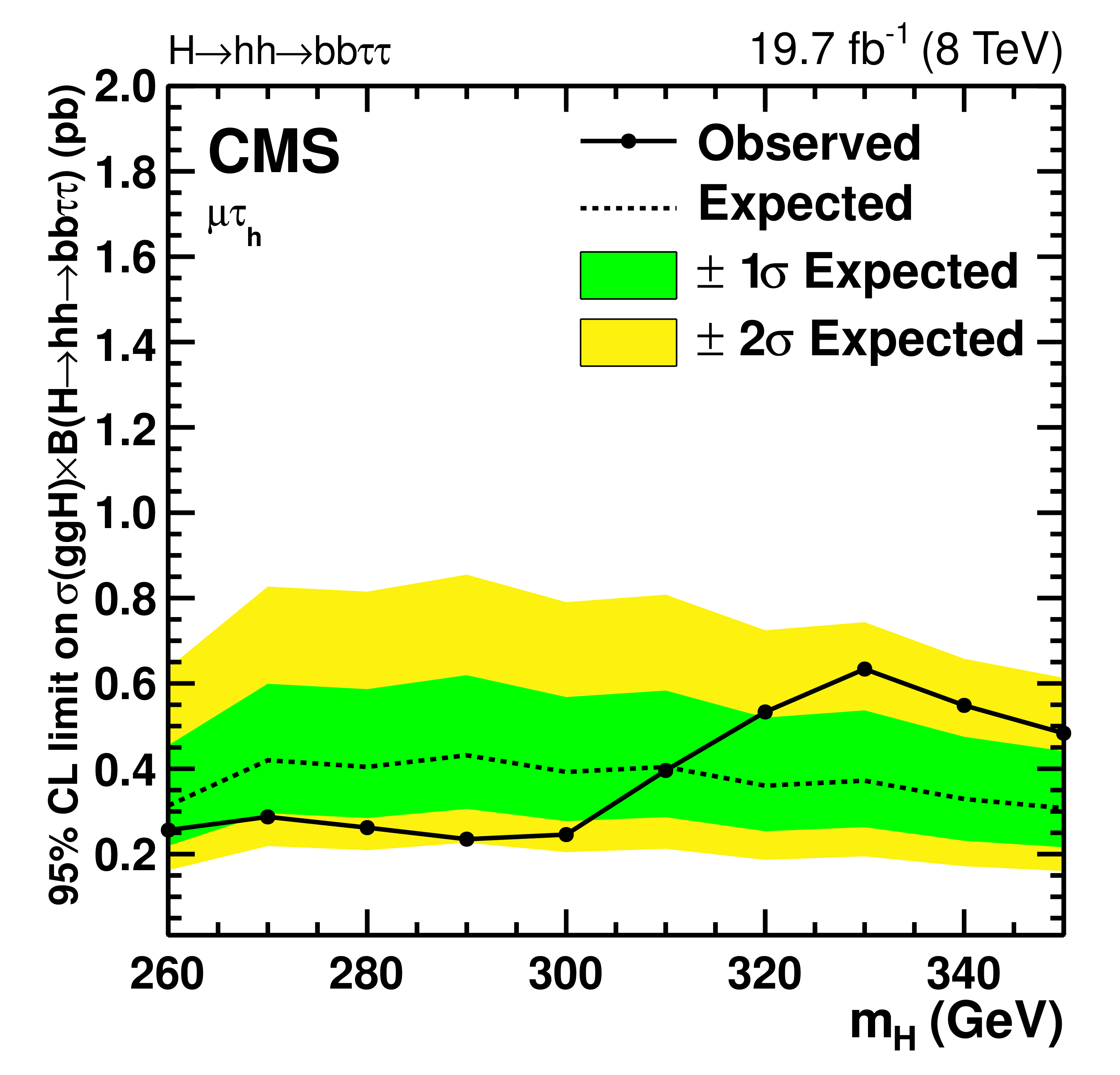
png pdf	Figure 8-a: Upper limits at 95% CL on the $\mathrm{h} \to \mathrm{h} \mathrm{h} \to \mathrm{b} \mathrm{b} \tau \tau $ cross section times branching fraction for the $\mu {\tau _\mathrm{h} } $ (a), $\mathrm{e} {\tau _\mathrm{h} } $ (b), $ {\tau _\mathrm{h} } {\tau _\mathrm{h} } $ (c), and for final states combined (d)
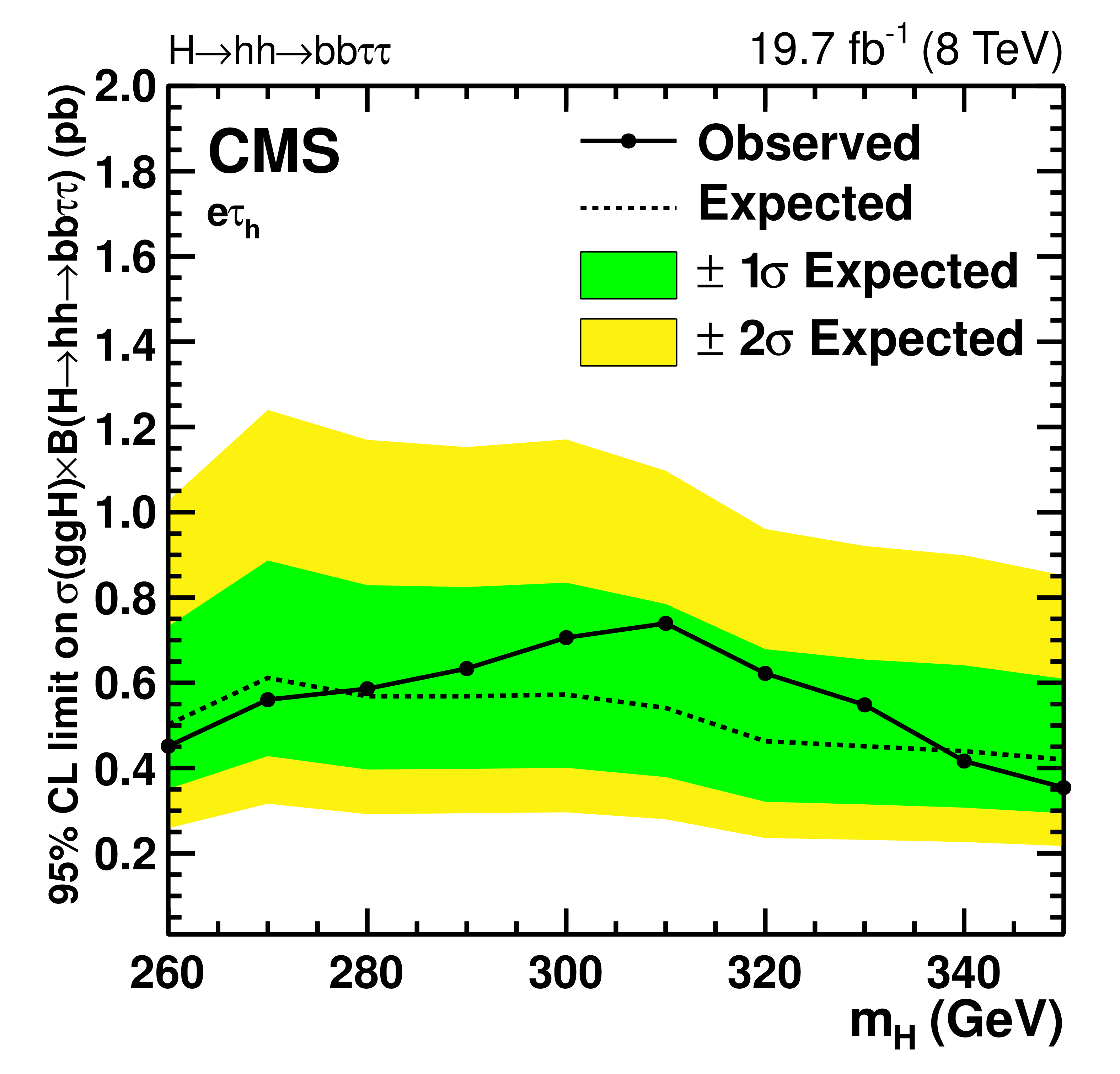
png pdf	Figure 8-b: Upper limits at 95% CL on the $\mathrm{h} \to \mathrm{h} \mathrm{h} \to \mathrm{b} \mathrm{b} \tau \tau $ cross section times branching fraction for the $\mu {\tau _\mathrm{h} } $ (a), $\mathrm{e} {\tau _\mathrm{h} } $ (b), $ {\tau _\mathrm{h} } {\tau _\mathrm{h} } $ (c), and for final states combined (d)
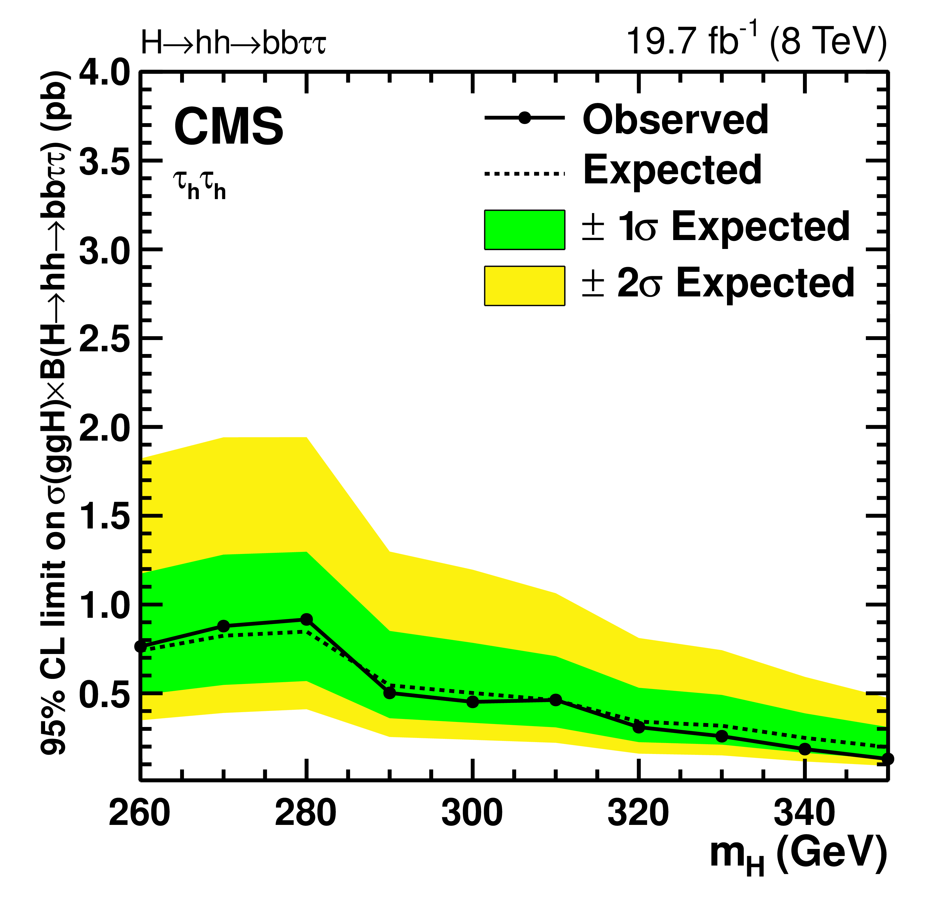
png pdf	Figure 8-c: Upper limits at 95% CL on the $\mathrm{h} \to \mathrm{h} \mathrm{h} \to \mathrm{b} \mathrm{b} \tau \tau $ cross section times branching fraction for the $\mu {\tau _\mathrm{h} } $ (a), $\mathrm{e} {\tau _\mathrm{h} } $ (b), $ {\tau _\mathrm{h} } {\tau _\mathrm{h} } $ (c), and for final states combined (d)
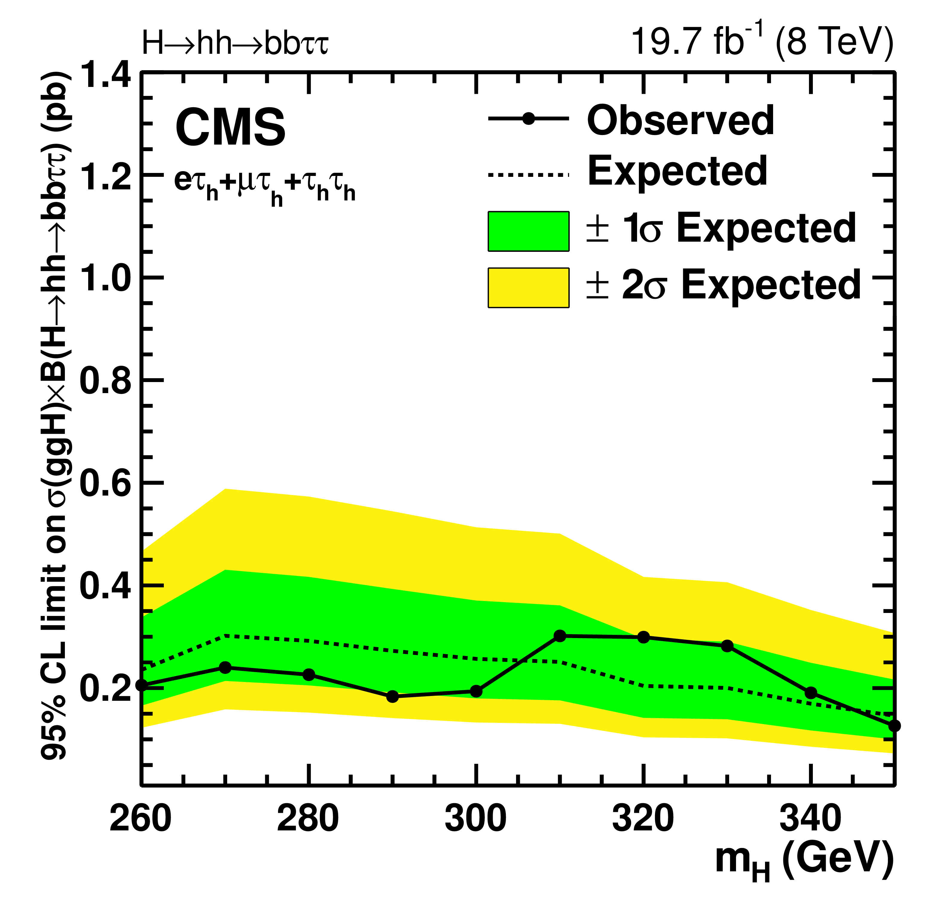
png pdf	Figure 8-d: Upper limits at 95% CL on the $\mathrm{h} \to \mathrm{h} \mathrm{h} \to \mathrm{b} \mathrm{b} \tau \tau $ cross section times branching fraction for the $\mu {\tau _\mathrm{h} } $ (a), $\mathrm{e} {\tau _\mathrm{h} } $ (b), $ {\tau _\mathrm{h} } {\tau _\mathrm{h} } $ (c), and for final states combined (d)
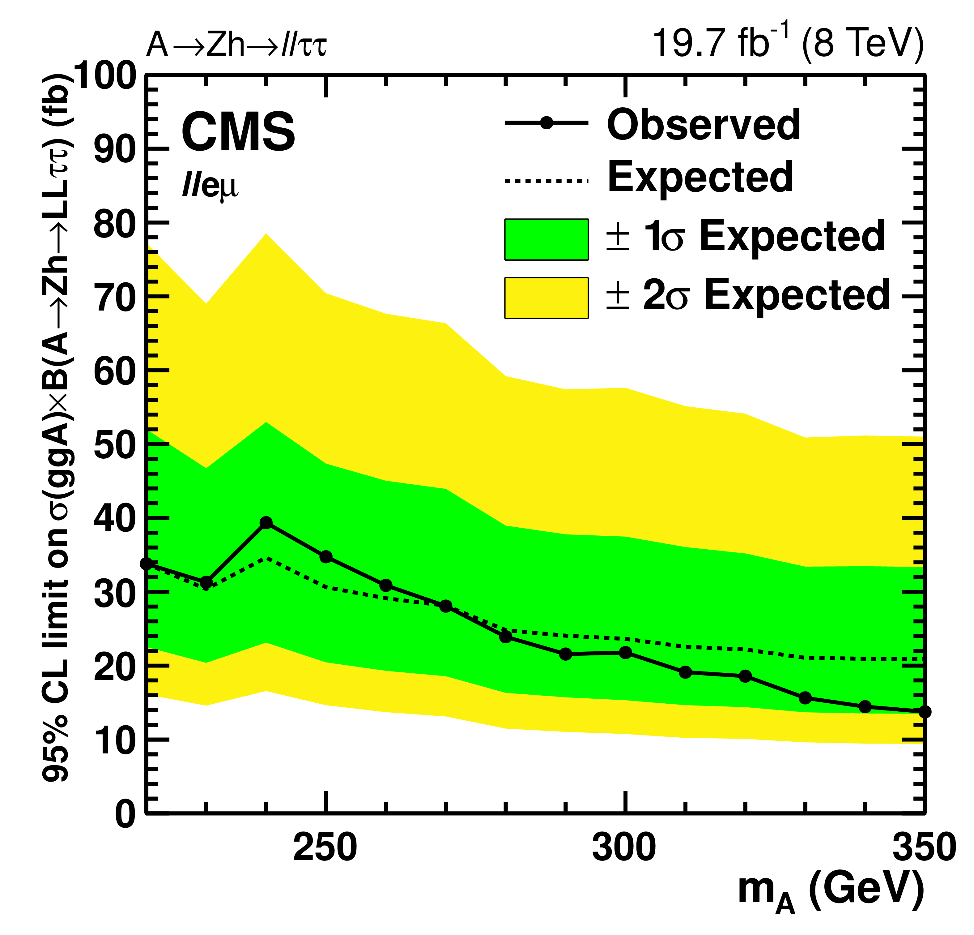
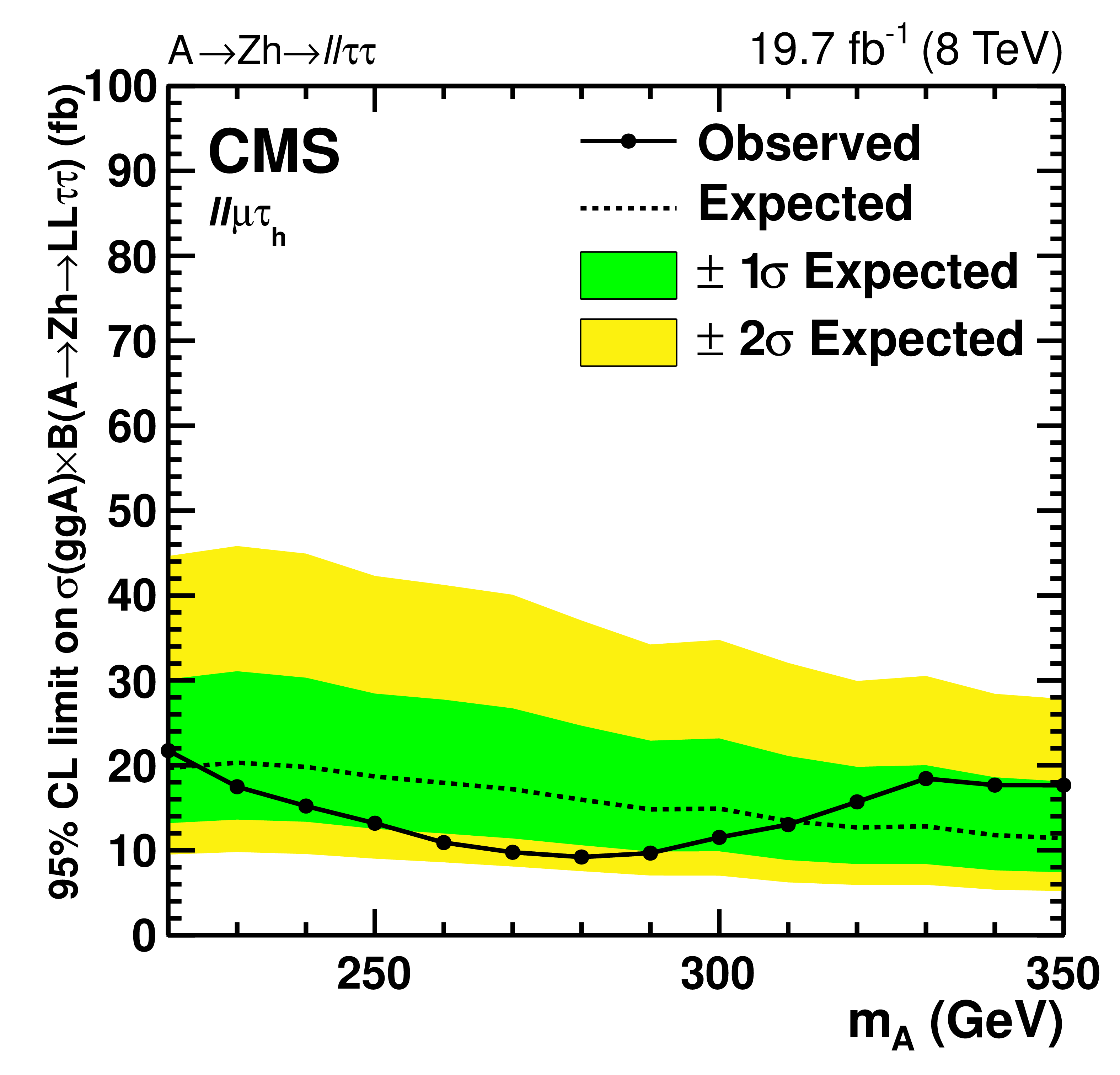
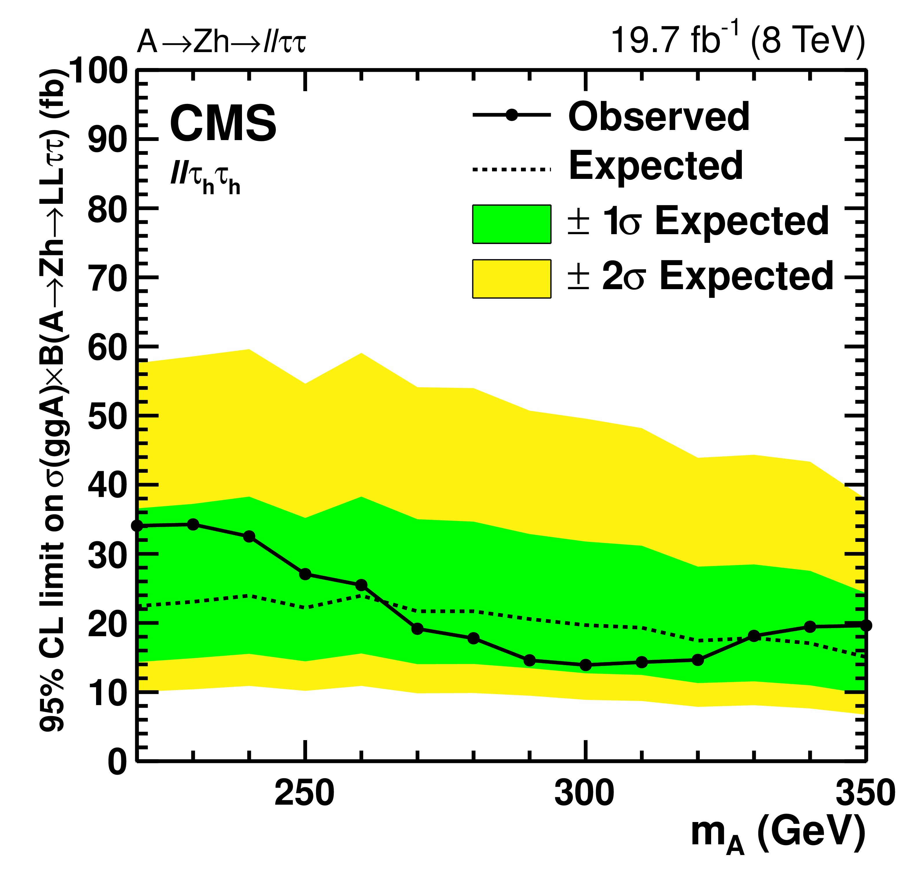
png pdf	Figure 9-a: Upper limits at 95% CL on cross section times branching fraction on $ {\mathrm {A}} \to \mathrm{Z} \mathrm{h} \to LL\tau \tau $ for $\ell \ell \mathrm{e} \mu $ (a), $\ell \ell \mu {\tau _\mathrm{h} } $ (b), $\ell \ell \mathrm{e} {\tau _\mathrm{h} } $ (c), and $\ell \ell {\tau _\mathrm{h} } {\tau _\mathrm{h} } $ (d) final states.
png pdf	Figure 9-b: Upper limits at 95% CL on cross section times branching fraction on $ {\mathrm {A}} \to \mathrm{Z} \mathrm{h} \to LL\tau \tau $ for $\ell \ell \mathrm{e} \mu $ (a), $\ell \ell \mu {\tau _\mathrm{h} } $ (b), $\ell \ell \mathrm{e} {\tau _\mathrm{h} } $ (c), and $\ell \ell {\tau _\mathrm{h} } {\tau _\mathrm{h} } $ (d) final states.
png pdf	Figure 9-c: Upper limits at 95% CL on cross section times branching fraction on $ {\mathrm {A}} \to \mathrm{Z} \mathrm{h} \to LL\tau \tau $ for $\ell \ell \mathrm{e} \mu $ (a), $\ell \ell \mu {\tau _\mathrm{h} } $ (b), $\ell \ell \mathrm{e} {\tau _\mathrm{h} } $ (c), and $\ell \ell {\tau _\mathrm{h} } {\tau _\mathrm{h} } $ (d) final states.
png pdf	Figure 9-d: Upper limits at 95% CL on cross section times branching fraction on $ {\mathrm {A}} \to \mathrm{Z} \mathrm{h} \to LL\tau \tau $ for $\ell \ell \mathrm{e} \mu $ (a), $\ell \ell \mu {\tau _\mathrm{h} } $ (b), $\ell \ell \mathrm{e} {\tau _\mathrm{h} } $ (c), and $\ell \ell {\tau _\mathrm{h} } {\tau _\mathrm{h} } $ (d) final states.
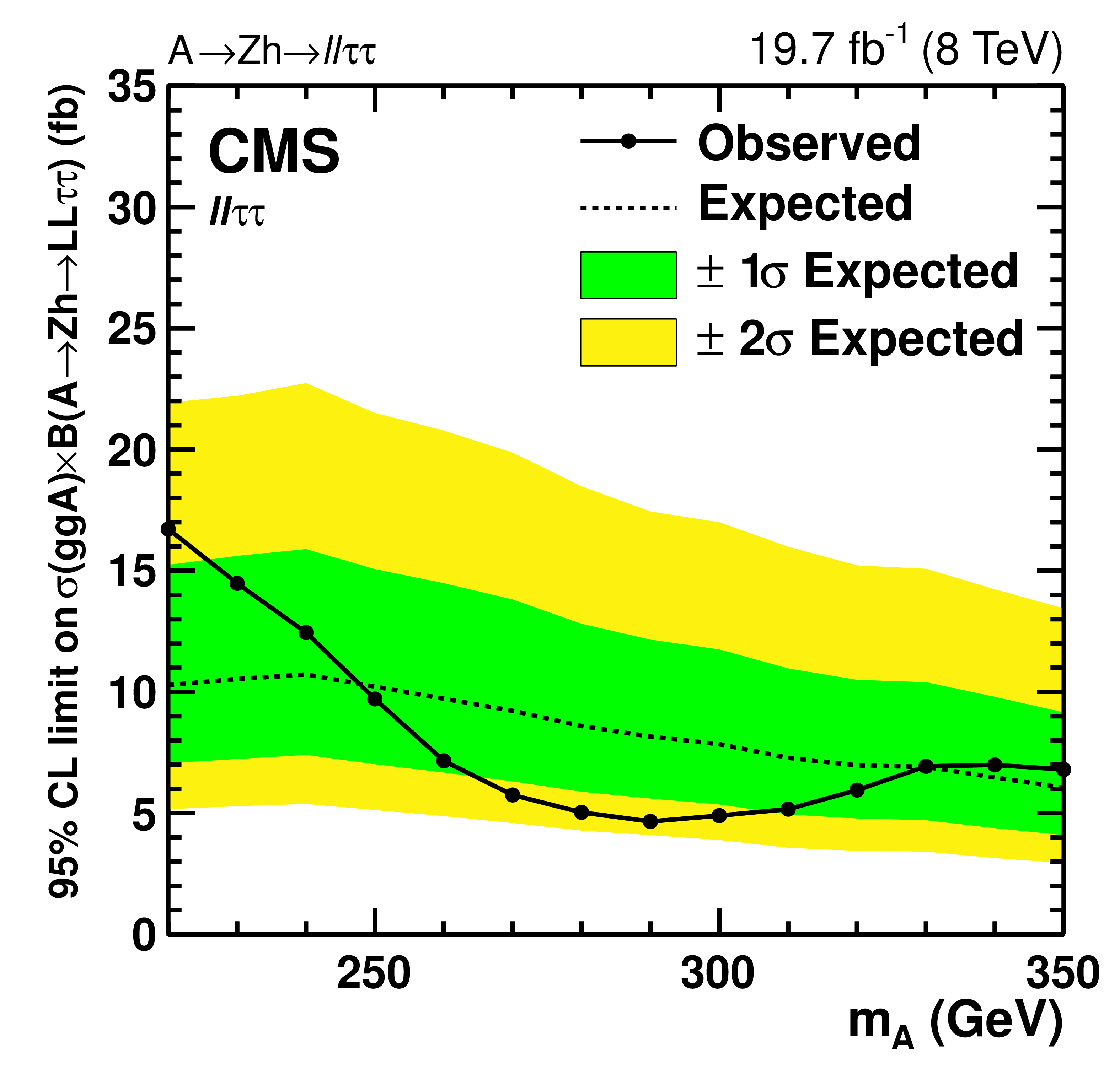
png pdf	Figure 10-a: Upper limits at 95% CL on cross section times branching fraction on $ {\mathrm {A}} \to \mathrm{Z} \mathrm{h} \to LL \tau \tau $ for all ${\ell \ell }\tau \tau $ final states combined (a) and comparison of the different final states (b).
png pdf	Figure 10-b: Upper limits at 95% CL on cross section times branching fraction on $ {\mathrm {A}} \to \mathrm{Z} \mathrm{h} \to LL \tau \tau $ for all ${\ell \ell }\tau \tau $ final states combined (a) and comparison of the different final states (b).
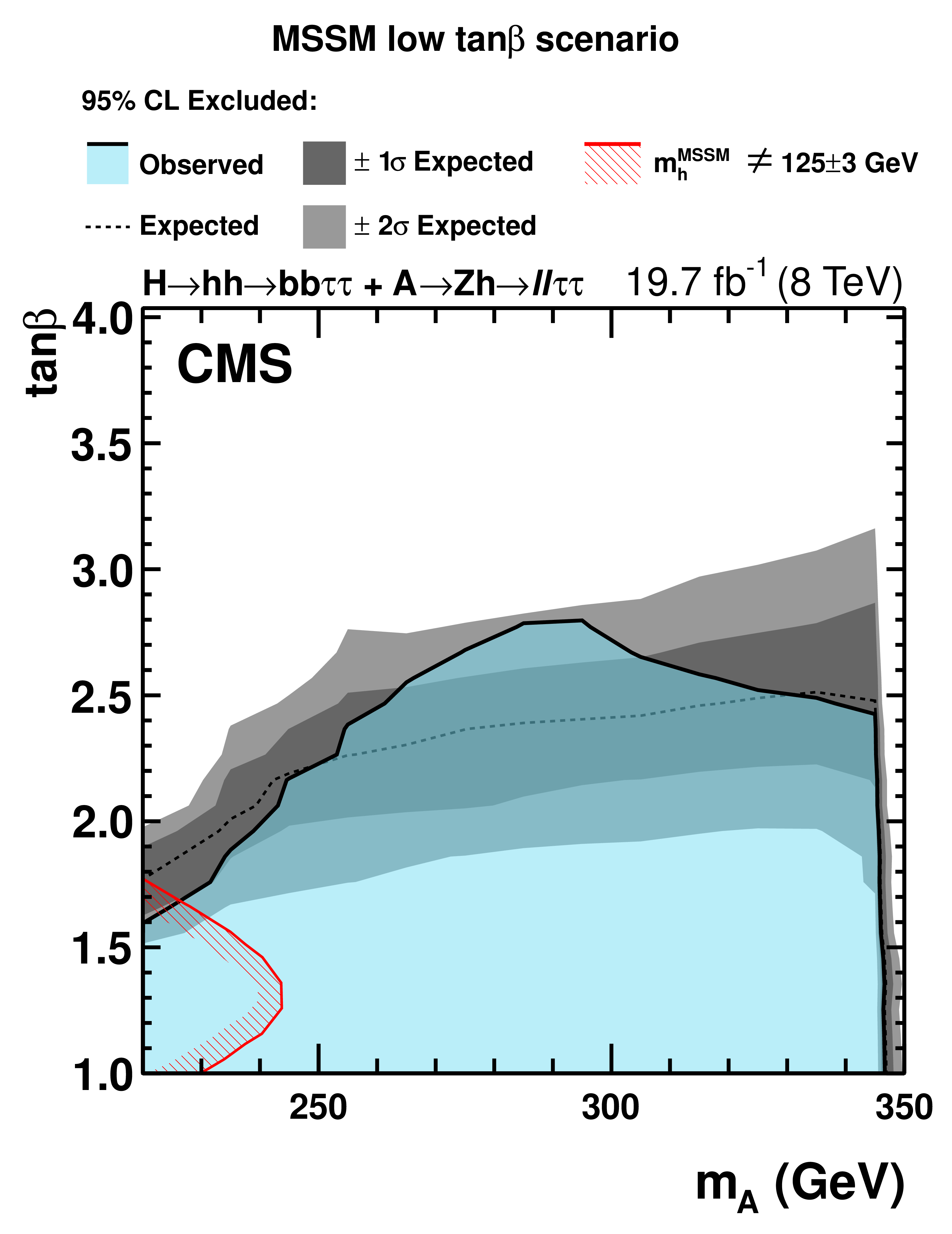
png pdf	Figure 11: The 95% CL exclusion region in the $m_ {\mathrm {A}} $-$\tan\beta $ plane for the low-$\tan\beta $ scenario as discussed in the introduction, combining the results of the $\mathrm{h} \to \mathrm{h} \mathrm{h} \to \mathrm{b} \mathrm{b} \tau \tau $ and the $ {\mathrm {A}} \to \mathrm{Z} \mathrm{h} \to {\ell \ell }\tau \tau $ analysis. The area highlighted in blue below the black curve marks the observed exclusion. The dashed curve and the grey bands show the expected exclusion limit with the relative uncertainty. The red area with the back-slash lines at the lower-left corner of the plot indicates the region excluded by the mass of the SM-like scalar boson being 125 GeV. The limit falls off rapidly as $m_ {\mathrm {A}} $ approaches 350 GeV because decays of the $ {\mathrm {A}} $ to two top quarks are becoming kinematically allowed.
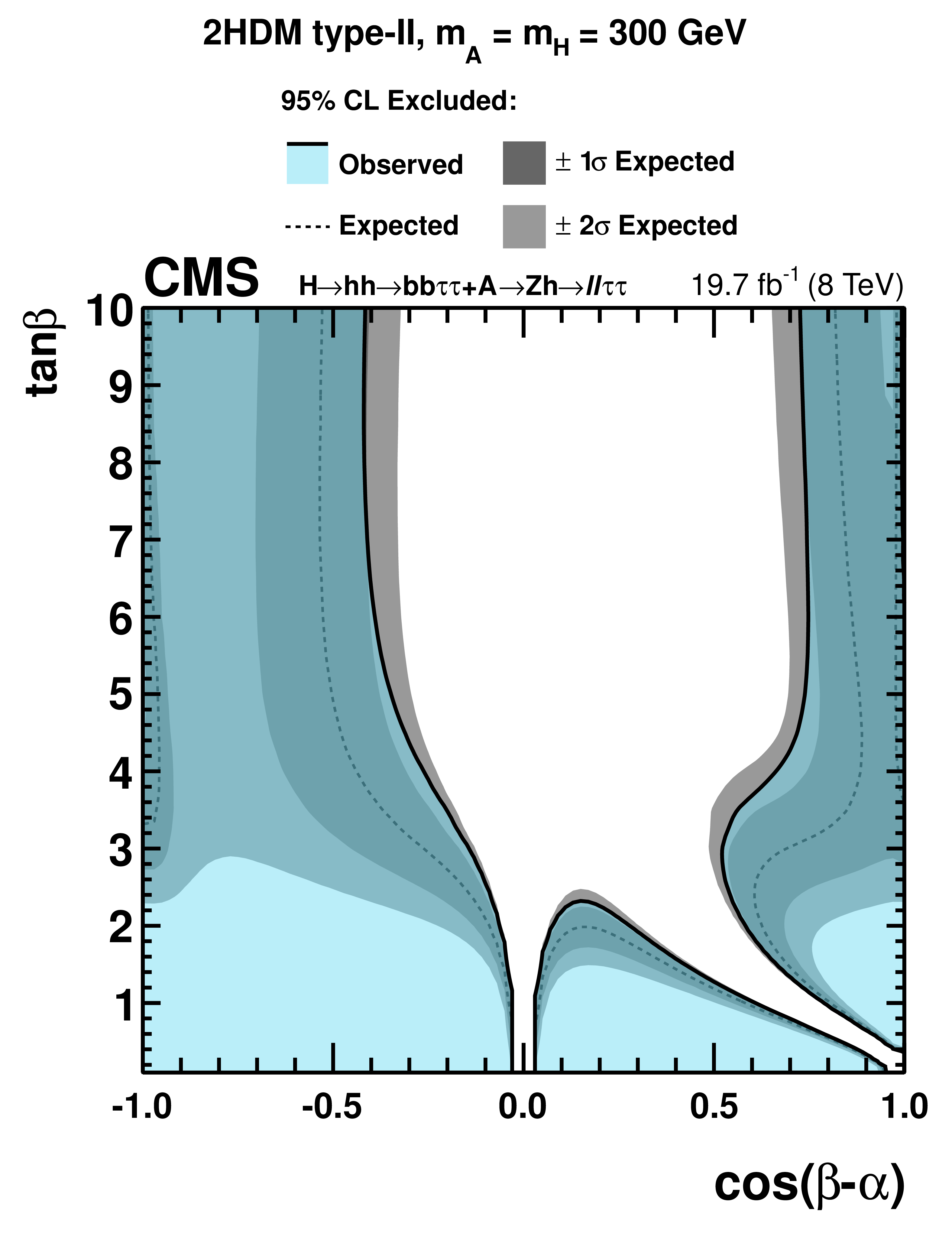
png pdf	Figure 12: The 95% CL exclusion regions in the $\cos(\beta -\alpha )$ vs. $\tan\beta $ plane of 2HDM Type II model for $m_{ {\mathrm {A}} }=m_{\mathrm{h} }=300$ GeV, combining the results of the $\mathrm{h} \to \mathrm{h} \mathrm{h} \to \mathrm{b} \mathrm{b} \tau \tau $ and $ {\mathrm {A}} \to \mathrm{Z} \mathrm{h} \to \ell \ell \tau \tau $ analysis. The areas highlighted in blue bounded by the black curves mark the observed exclusion. The dashed curves and the grey bands show the expected exclusion limit with the relative uncertainty.

Summary

A search for a heavy scalar Higgs boson ($ \mathrm{H} $) decaying into a pair of SM-like Higgs bosons ($ \mathrm{hh} $) and a search for a heavy neutral pseudoscalar Higgs boson ($ \mathrm{A} $) decaying into a $ \mathrm{Z} $ boson and a SM-like Higgs boson ($ \mathrm{h} $), have been performed using events recorded by the CMS experiment at the LHC. The dataset corresponds to an integrated luminosity of 19.7 fb$^{-1}$, recorded at 8 TeV centre-of-mass energy in 2012. No evidence for a signal has been found and exclusion limits on the production cross section times branching fraction for the processes $ \mathrm{H \to h h \to b b \tau \tau } $ and $ \mathrm{ A \to Zh \to L L \tau \tau } $ are presented. The results are also interpreted in the context of the MSSM and 2HDM models.

Additional Figures
png pdf	Additional Figure 1: Observed and predicted m$_{A}$ distributions in the $\ell \ell + e\mu$ channel, for the A $\rightarrow$ Zh $\rightarrow \ell\ell\tau\tau$ analysis. The normalization of the predicted background distributions corresponds to the result of the global fit. The signal distribution is normalized to the MSSM low-tan$\beta$ scenario with tan $\beta$=2.
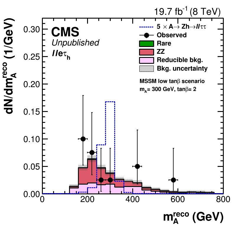
png pdf	Additional Figure 2: Observed and predicted m$_{A}$ distributions in the $\ell \ell+e\tau_h$ channel, for the A $\rightarrow$Zh $\rightarrow \ell\ell\tau\tau$ analysis. The normalization of the predicted background distributions corresponds to the result of the global fit. The signal distribution is normalized to the MSSM low-tan$\beta$ scenario with tan $\beta$=2.
png pdf	Additional Figure 3: Observed and predicted m$_{A}$ distributions in the $\ell \ell+\mu\tau_h$ channel, for the A $\rightarrow$ Zh$\rightarrow \ell\ell\tau\tau$ analysis. The normalization of the predicted background distributions corresponds to the result of the global fit. The signal distribution is normalized to the MSSM low-tan$\beta$ scenario with tan $\beta$=2.
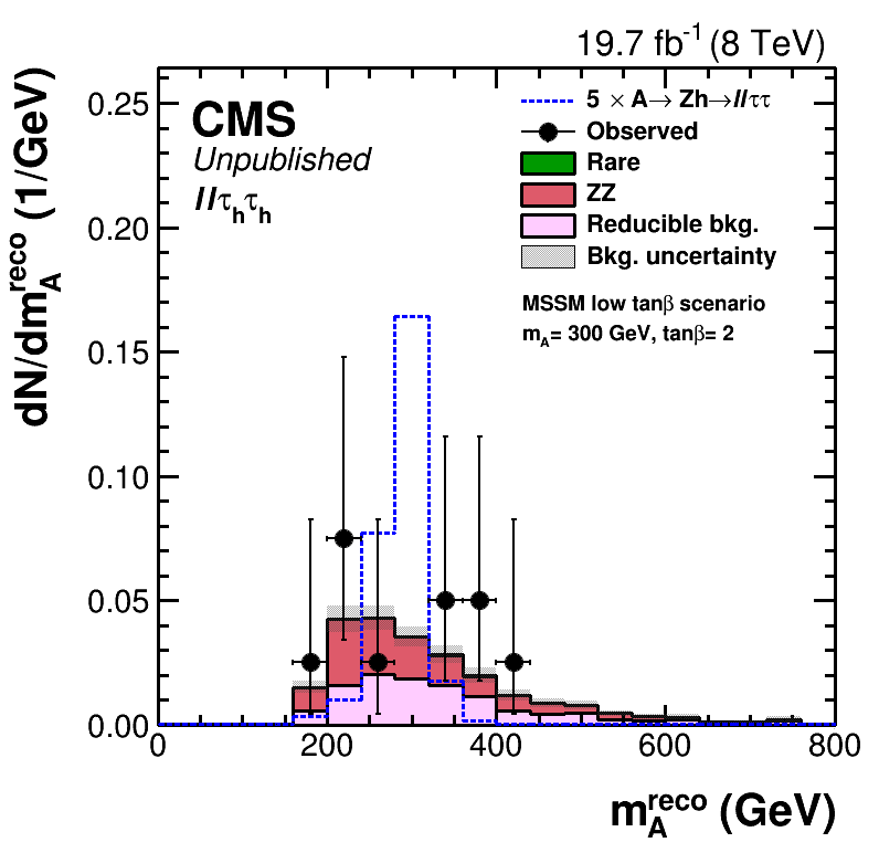
png pdf	Additional Figure 4: Observed and predicted m$_{A}$ distributions in the $\ell \ell+\tau_h\tau_h$ channel, for the A $\rightarrow$Zh$\rightarrow \ell\ell\tau\tau$ analysis. The normalization of the predicted background distributions corresponds to the result of the global fit. The signal distribution is normalized to the MSSM low-tan$\beta$ scenario with tan $\beta=2$.
png pdf	Additional Figure 5: Observed and predicted m$_{A}$ distributions in all eight final states combined, for the A $\rightarrow$ Zh$\rightarrow \ell\ell\tau\tau$ analysis. The normalization ofthe predicted background distributions corresponds to the result of the global fit. The signal distribution is normalized to the MSSM low-tan$\beta$ scenario with tan $\beta$=2.
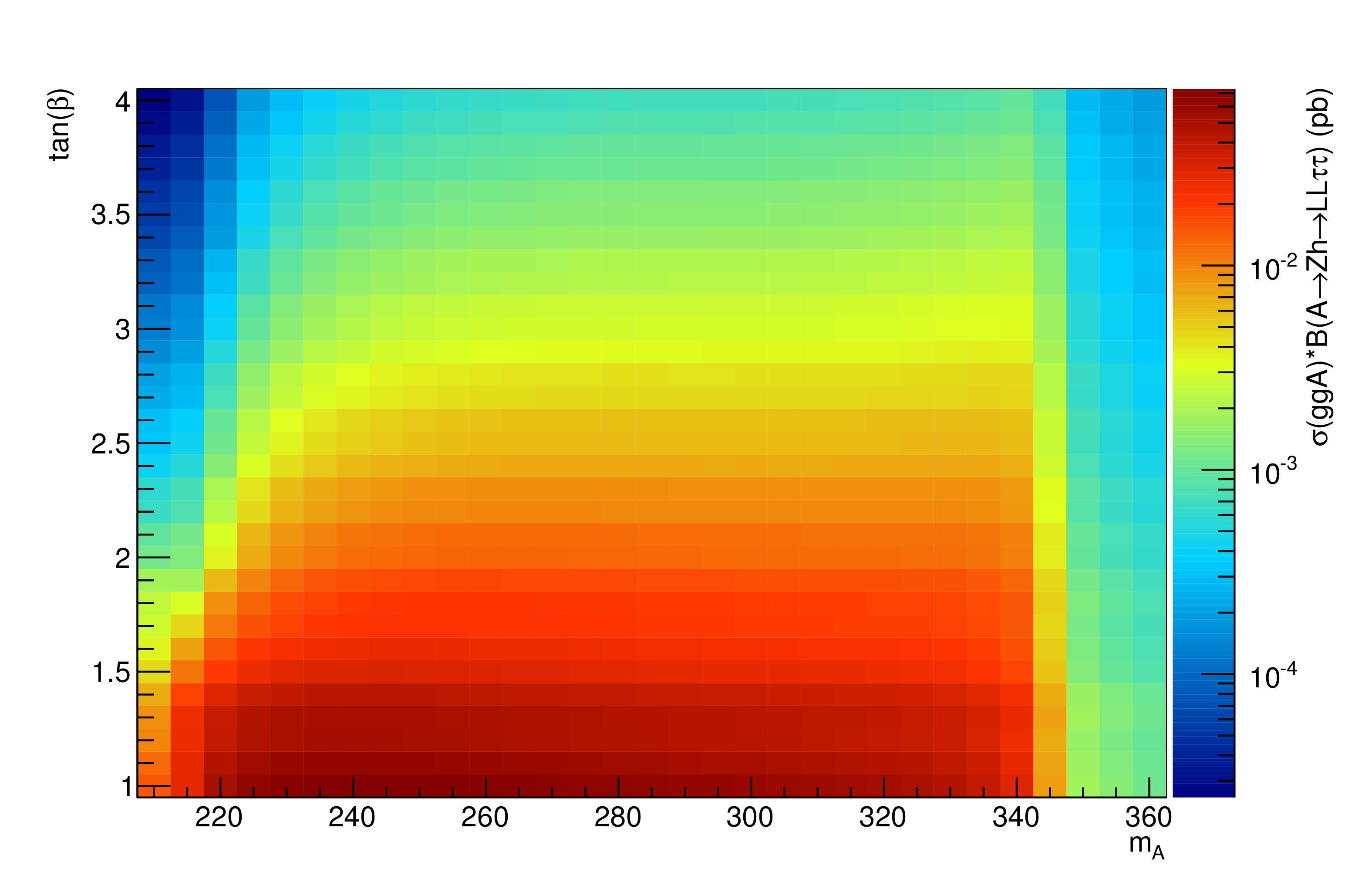
png pdf	Additional Figure 6: Values of cross-section times branching ratio for the A$\rightarrow$Zh$\rightarrow$LL$\tau\tau$ process in the low-tan$\beta$ scenario. The points indicate the values available from the theoretical calculations.
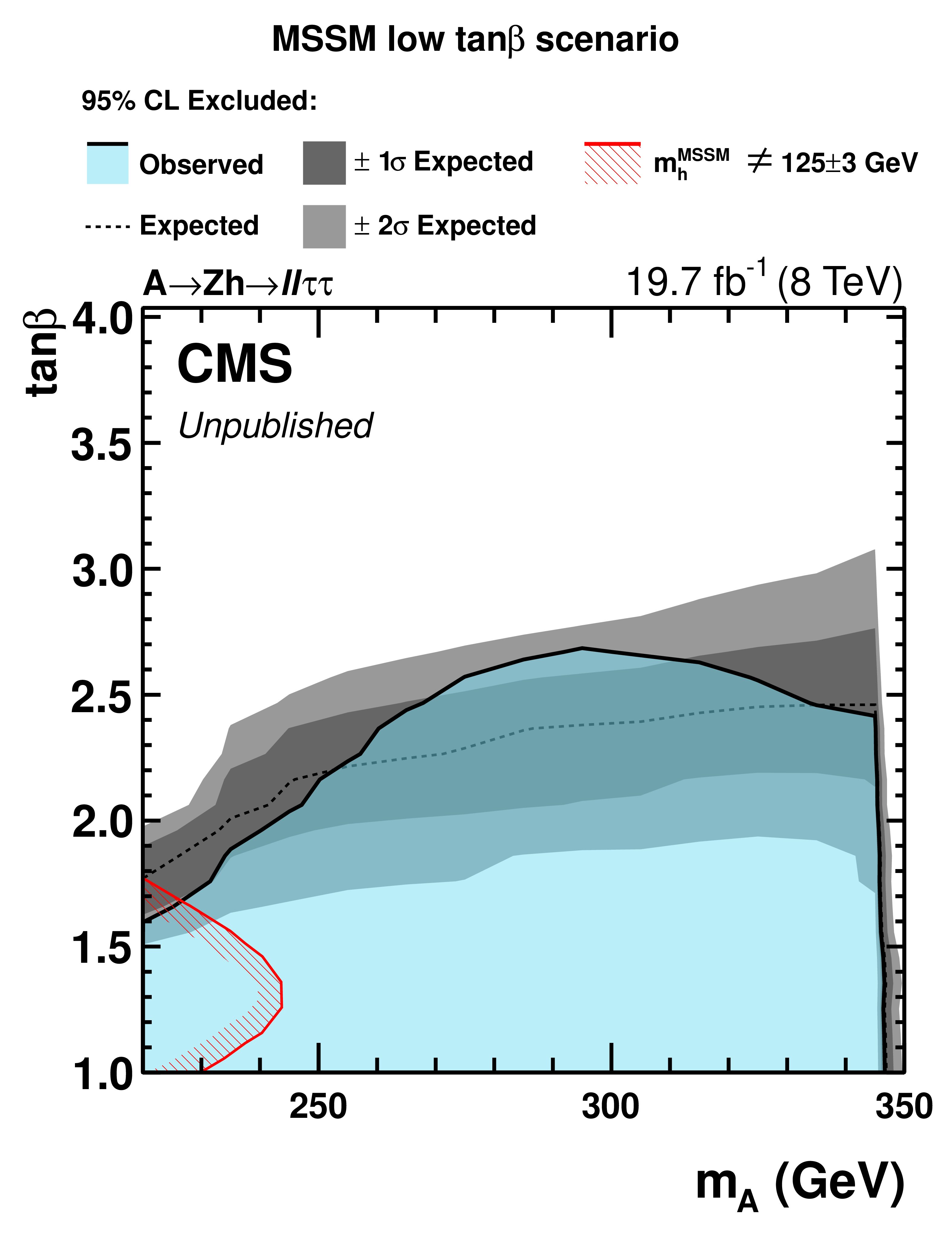
png pdf	Additional Figure 7: The 95% CL exclusion region in the m$_{A}$ - tan$\beta$ plane for the low-tan$\beta$ scenario as discussed in the introduction, using the results of the A $\rightarrow$ Zh $\rightarrow$ $\ell\ell\tau\tau$ analysis. The red area indicates the region excluded by the mass of the SM-like scalar being inconsistent with 125 GeV.
png pdf	Additional Figure 8: Values of cross-section times branching ratio for the A$\rightarrow$Zh$\rightarrow$LL$\tau\tau$ process in 2HDM Type II model. The points indicate the values available from the theoretical calculations. Areas in white have a value lower than that indicated in the legend, and are far from exclusion.
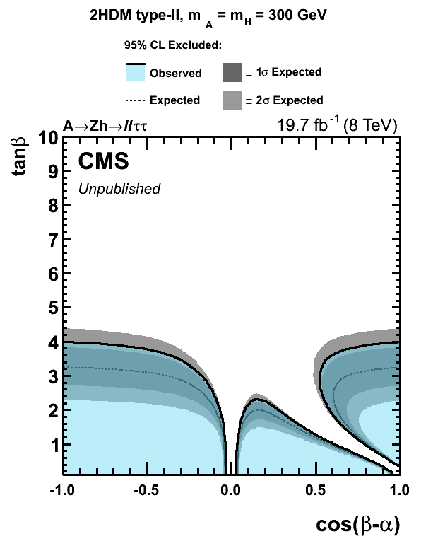
png pdf	Additional Figure 9: The 95% CL exclusion regions in the $cos(\beta - \alpha)$ - tan$ \beta$ plane of 2HDM Type II model for m$_{A}$ = m$_{H}$ = 300 GeV, using the results of the A $\rightarrow$ Zh$\rightarrow$ $\ell\ell\tau\tau$ analysis.
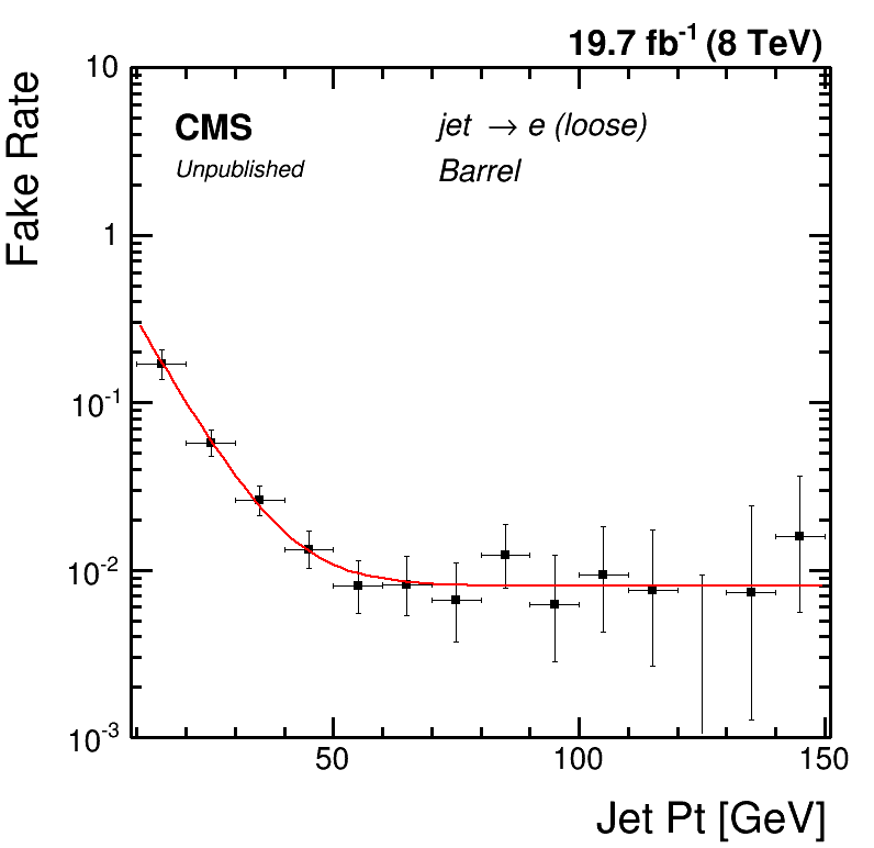
png pdf	Additional Figure 10: Rate with which jets are misidentified as electrons, in $\ell\ell + e\mu$ final states, in the barrel, as a function of the p$_{\rm{T}}$ of the closest jet to the electron for A $\rightarrow$ Zh $\rightarrow$ $\ell\ell\tau\tau$ analysis.
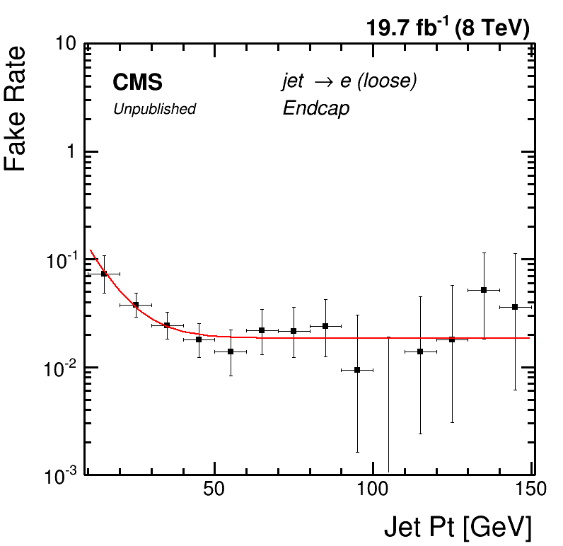
png pdf	Additional Figure 11: Rate with which jets are identified as electrons, in $\ell\ell + e\mu$ final states, in the endcap, as a function of the p$_{\rm{T}}$ of the closest jet to the electron for A $\rightarrow$ Zh$\rightarrow$ $\ell\ell\tau\tau$ analysis.
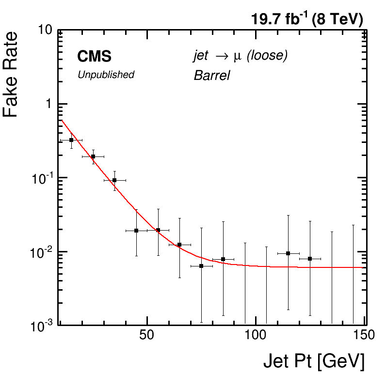
png pdf	Additional Figure 12: Rate with which jets are misidentified as muons, in $\ell\ell + e\mu$ final states, in the barrel, as a function of the p$_{\rm{T}}$ of the closest jet to the muon for A $\rightarrow$ Zh$\rightarrow$ $\ell\ell\tau\tau$ analysis.
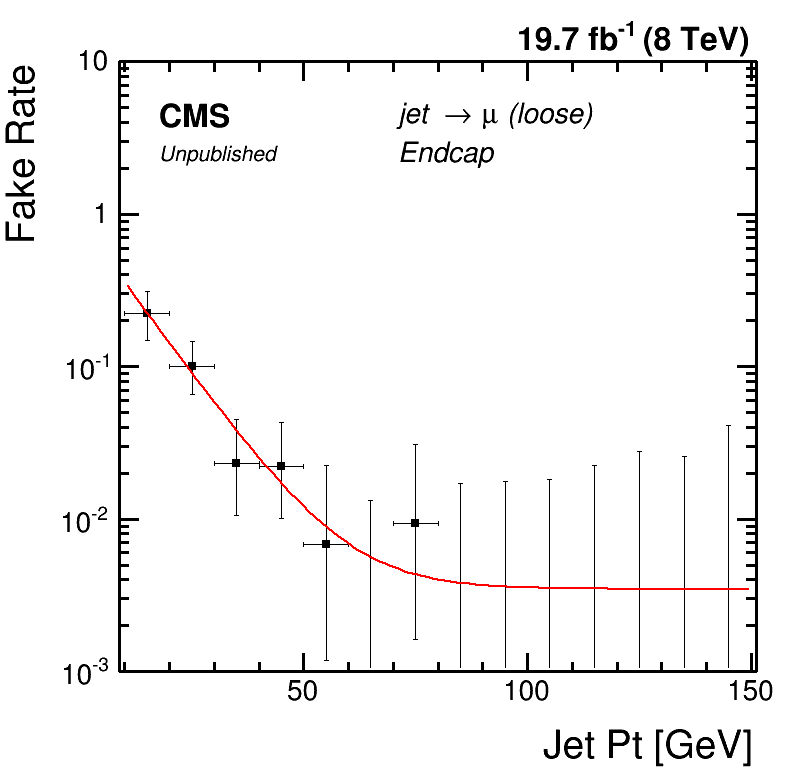
png pdf	Additional Figure 13: Rate with which jets are misidentified as muons, in $\ell\ell + e\mu$ final states, in the endcap, as a function of the p$_{\rm{T}}$ of the closest jet to the muon for A $\rightarrow$ Zh$\rightarrow$ $\ell\ell\tau\tau$ analysis.
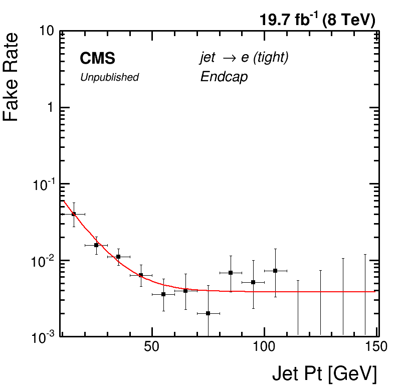
png pdf	Additional Figure 14: Rate with which jets are misidentified as electrons, in $\ell\ell + e\tau_h$ final states, in the endcap, as a function of the p$_{\rm{T}}$ of the closest jet to the electron forA $\rightarrow$ Zh $\rightarrow$ $\ell\ell\tau\tau$ analysis.
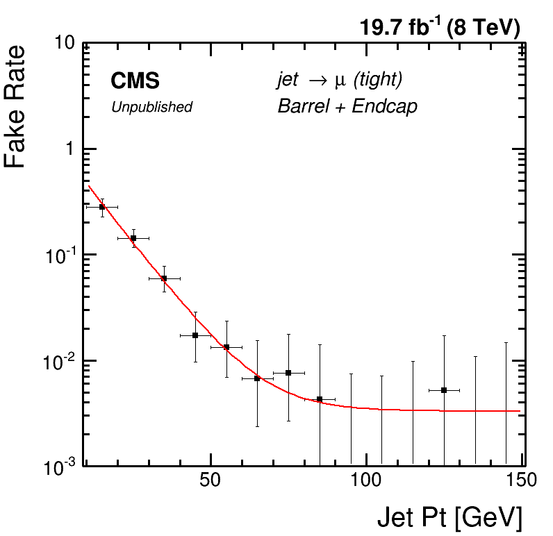
png pdf	Additional Figure 15: Rate with which jets are misidentified as muons, in $\ell\ell + \mu\tau_h$ final states, in the barrel and the endcap regions combined, as a function of the p$_{\rm{T}}$ of the closest jet to the muon for A $\rightarrow$ Zh$\rightarrow$ $\ell\ell\tau\tau$ analysis.
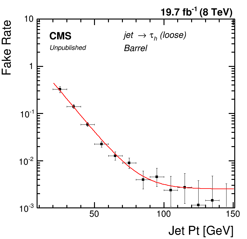
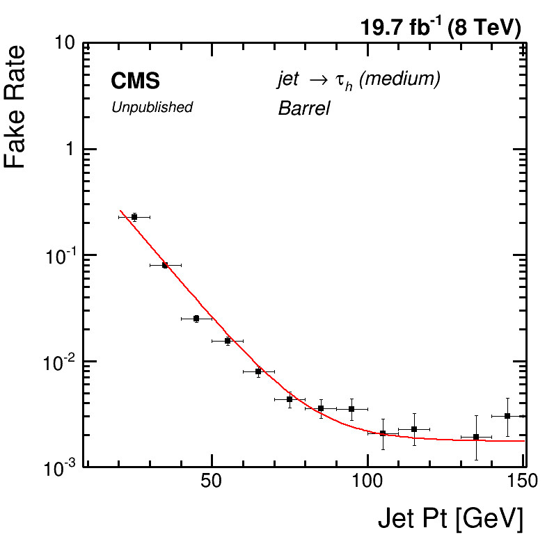
png pdf	Additional Figure 16: Rate with which jets are misidentified as hadronically decaying taus, in $\ell\ell + \ell\tau_h$ final states, in the barrel, as a function of the p$_{\rm{T}}$ of the closest jet to the tau for A $\rightarrow$ Zh$\rightarrow$ $\ell\ell\tau\tau$ analysis.
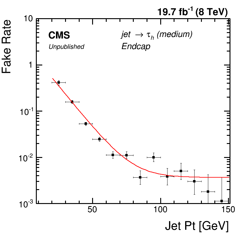
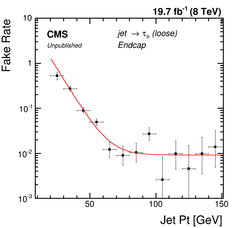
png pdf	Additional Figure 17: Rate with which jets are misidentified as hadronically decaying taus, in $\ell\ell + \ell\tau_h$ final states, in the endcap, as a function of the p$_{\rm{T}}$ of the closest jet to the tau for A $\rightarrow$ Zh$\rightarrow$ $\ell\ell\tau\tau$ analysis.
png pdf	Additional Figure 18: Rate with which jets are misidentified as hadronically decaying taus, in $\ell \ell + \tau_h\tau_h$ final states, in the barrel, as a function of the p$_{\rm{T}}$ of the closest jet to the tau for A $\rightarrow$ Zh analysis.
png pdf	Additional Figure 19: Rate with which jets are misidentified as hadronically decaying taus, in $ll + \tau_h\tau_h$ final states, in the endcap, as a function of the p$_{\rm{T}}$ of the closest jet to the tau for A $\rightarrow$ Zh analysis.
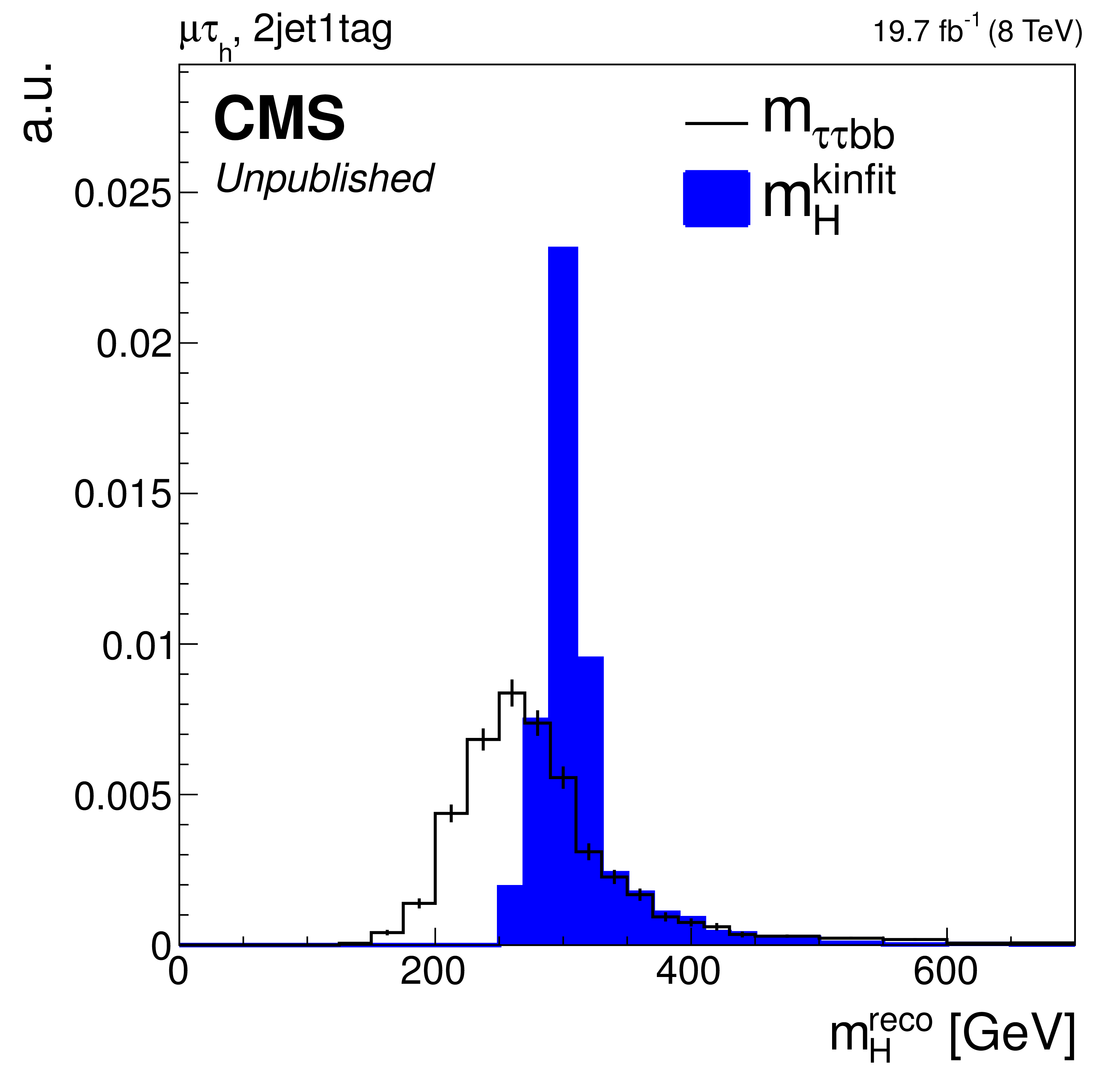
png pdf	Additional Figure 20: Comparison between 4-body mass distribution with and without the kinematic fit applied for signal events in the $\mu\tau_{h}$ channel and 2jet-1tag category of the H$\rightarrow$hh$\rightarrow$ bb$\tau\tau$ analysis with m$_{H}$ = 300 GeV.
png pdf	Additional Figure 21: Mass of the candidate di-tau pair m$_{\tau\tau}$ for events in the $\mu\tau_{h}$ final state and 2jet-1tag category of the H$\rightarrow$hh$\rightarrow$ bb$\tau\tau$ analysis. Events in a window around m$_{h}$=125 GeV of 90 $<$ m$_{\tau\tau}$ $<$ 150 GeV are used for signal extraction.
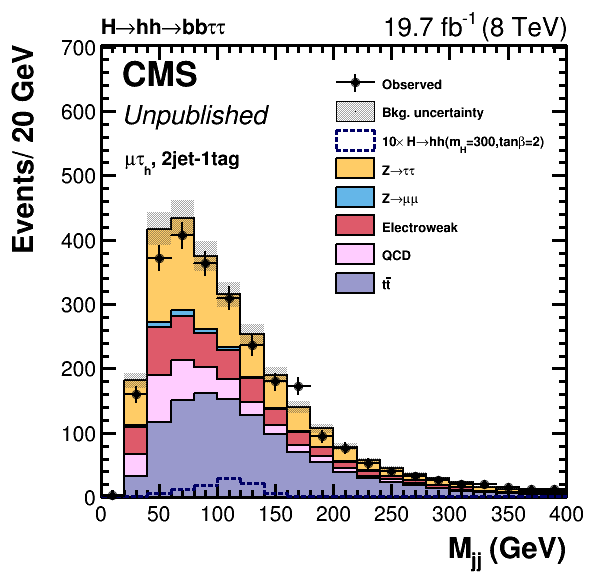
png pdf	Additional Figure 22: Mass of the candidate di-jet pair m$_{jj}$ for events in the $\mu\tau_{h}$ final state and 2jet-1tag category of the H$\rightarrow$hh$\rightarrow$ bb$\tau\tau$ analysis. Events in a window around m$_{h}$=125 GeV of 70 $<$ m$_{jj}$ $<$ 150 GeV are used for signal extraction.
png pdf	Additional Figure 23: Mass of the candidate di-tau pair m$_{\tau\tau}$ for events in the $\mu\tau_{h}$ final state and 2jet-2tag category of the H$\rightarrow$hh$\rightarrow$ bb$\tau\tau$ analysis. Events in a window around m$_{h}$=125 GeV of 90 $<$ m$_{\tau\tau}$ $<$ 150 GeV are used for signal extraction.
png pdf	Additional Figure 24: Mass of the candidate di-jet pair m$_{jj}$ for events in the $\mu\tau_{h}$ final state and 2jet-2tag category of the H$\rightarrow$hh$\rightarrow$ bb$\tau\tau$ analysis. Events in a window around m$_{h}$=125 GeV of 70 $<$ m$_{jj}$ $<$ 150 GeV are used for signal extraction.
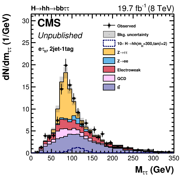
png pdf	Additional Figure 25: Mass of the candidate di-tau pair m$_{\tau\tau}$ for events in the $e\tau_{h}$ final state and 2jet-1tag category of the H$\rightarrow$hh$\rightarrow$ bb$\tau\tau$ analysis. Events in a window around m$_{h}$=125 GeV of 90 $<$ m$_{\tau\tau}$ $<$ 150 GeV are used for signal extraction.
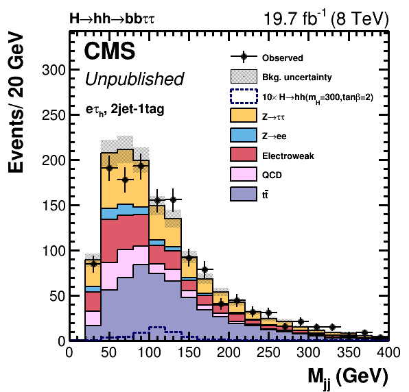
png pdf	Additional Figure 26: Mass of the candidate di-jet pair m$_{jj}$ for events in the $e\tau_{h}$ final state and 2jet-1tag category of the H$\rightarrow$hh$\rightarrow$ bb$\tau\tau$ analysis. Events in a window around m$_{h}$=125 GeV of 70 $<$ m$_{jj}$ $<$ 150 GeV are used for signal extraction.
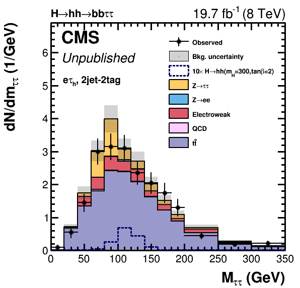
png pdf	Additional Figure 27: Mass of the candidate di-tau pair m$_{\tau\tau}$ for events in the $e\tau_{h}$ final state and 2jet-2tag category of the H$\rightarrow$hh$\rightarrow$ bb$\tau\tau$ analysis. Events in a window around m$_{h}$=125 GeV of 90 $<$ $m_{\tau\tau}$ $<$ 150 GeV are used for signal extraction.
png pdf	Additional Figure 28: Mass of the candidate di-jet pair m$_{jj}$ for events in the $e\tau_{h}$ final state and 2jet-2tag category of the H$\rightarrow$hh$\rightarrow$ bb$\tau\tau$ analysis. Events in a window around m$_{h}$=125 GeV of 70 $<$ m$_{jj}$ $<$ 150 GeV are used for signal extraction.
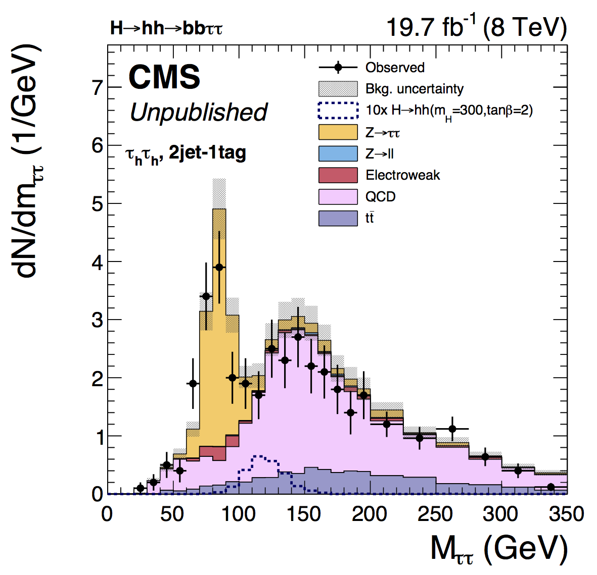
png pdf	Additional Figure 29: Mass of the candidate di-tau pair m$_{\tau\tau}$ for events in the $\tau_{h}\tau_{h}$ final state and 2jet-1tag category of the H$\rightarrow$hh$\rightarrow$ bb$\tau\tau$ analysis. Events in a window around m$_{h}$=125 GeV of 90 $<$ m$_{\tau\tau}$ $<$ 150 GeV are used for signal extraction.
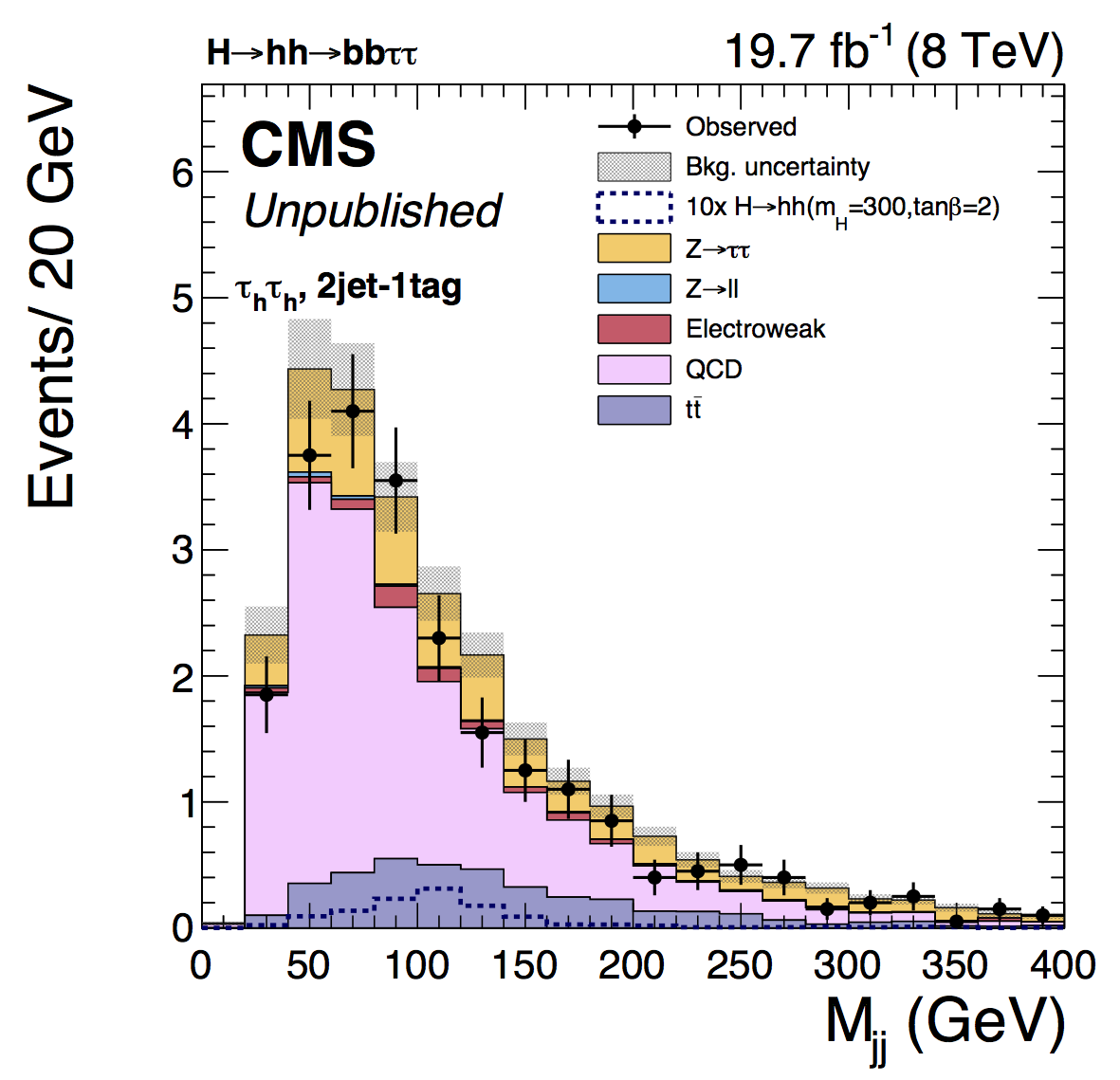
png pdf	Additional Figure 30: Mass of the candidate di-jet pair m$_{jj}$ for events in the $\tau_{h}\tau_{h}$ final state and 2jet-1tag category of the H$\rightarrow$hh$\rightarrow$ bb$\tau\tau$ analysis. Events in a window around m$_{h}$=125 GeV of 70 $<$ m$_{jj}$ $<$ 150 GeV are used for signal extraction.
png pdf	Additional Figure 31: Mass of the candidate di-tau pair m$_{\tau\tau}$ for events in the $\tau_{h}\tau_{h}$ final state and 2jet-2tag category of the H$\rightarrow$hh$\rightarrow$bb$\tau\tau$ analysis. Events in a window around m$_{h}$=125 GeV of 90 $<$ m$_{\tau\tau}$ $<$ 150 GeV are used for signal extraction.
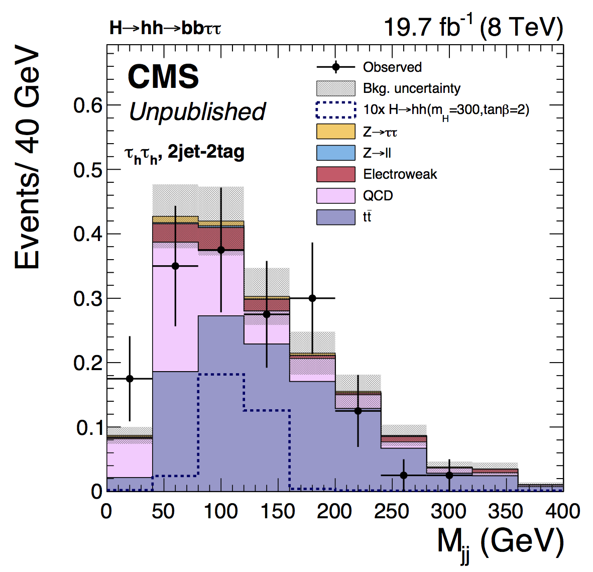
png pdf	Additional Figure 32: Mass of the candidate di-jet pair m$_{jj}$ for events in the $\tau_{h}\tau_{h}$ final state and 2jet-2tag category of the H$\rightarrow$hh$\rightarrow$ bb$\tau\tau$ analysis. Events in a window around m$_{h}$=125 GeV of 70 $<$ m$_{jj}$ $<$ 150 GeV are used for signal extraction.
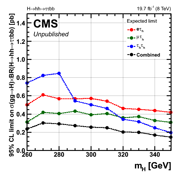
png pdf	Additional Figure 33: Comparison of the expected limits for the H$\rightarrow$hh$\rightarrow$ bb$\tau\tau$ analysis, separated by final state.
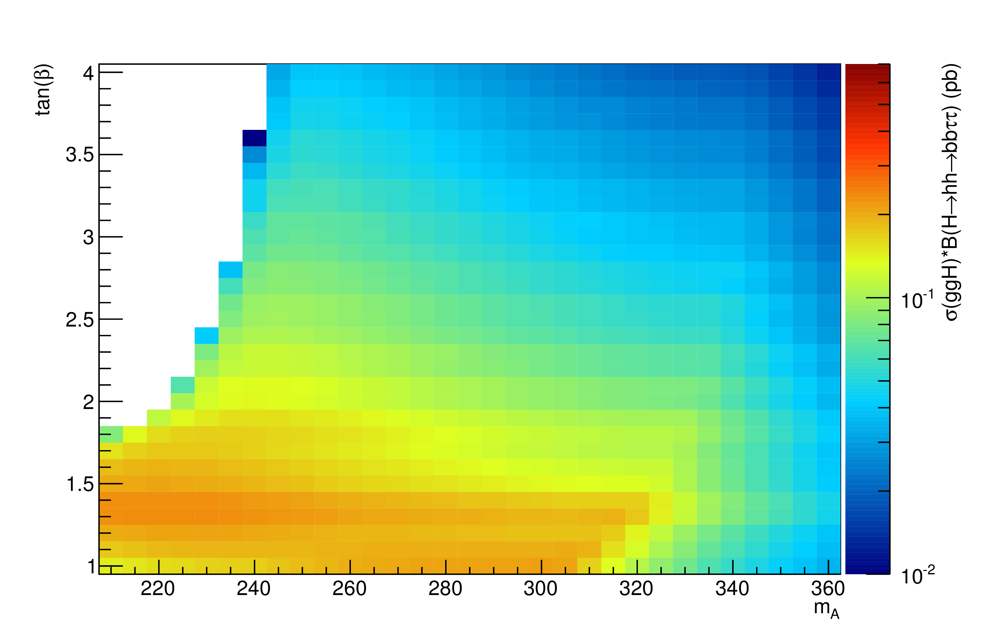
png pdf	Additional Figure 34: Values of cross-section times branching ratio for the H$\rightarrow$hh$\rightarrow$ bb$\tau\tau$ process in the in the m$_{A}$ -tan$\beta$ plane for the low-tan$\beta$ scenario. The points indicate the values available from the theoretical calculations. Areas in white have a value lower than that indicated in the legend, and are far from exclusion.
png pdf	Additional Figure 35: Values of cross-section times branching ratio for the H$\rightarrow$hh$\rightarrow$bb$\tau\tau$ process in the type 2 2HDM scenario. The points indicate the values available from the theoretical calculations. Areas in white have a value lower than that indicated in the legend, and are far from exclusion.
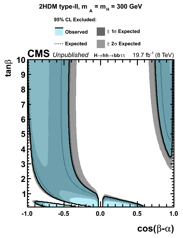
png pdf	Additional Figure 36: The 95% CL exclusion regions in the $cos(\beta - \alpha)$ - tan$\beta$ plane of 2HDM Type II model for m$_{A}$ = m$_{H}$ = 300 GeV, using the results of the H $\rightarrow$hh $\rightarrow$ bb$\tau\tau$ analysis
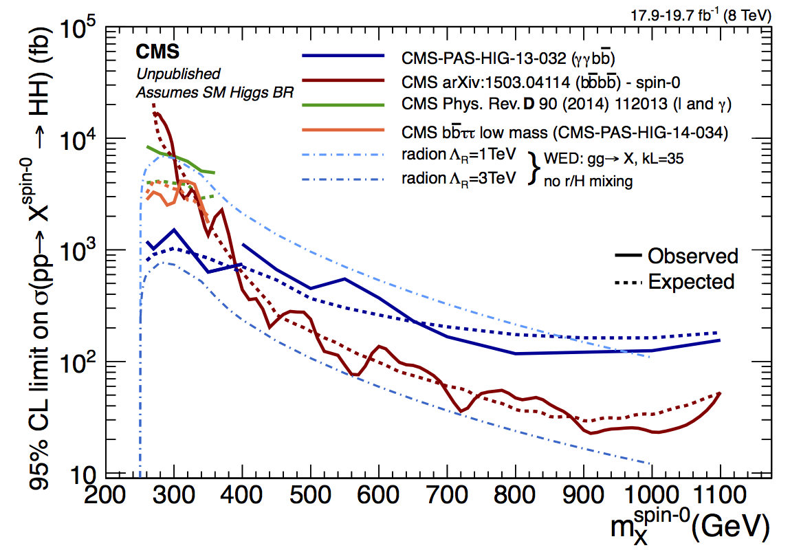
png pdf	Additional Figure 37: Comparison of limits on cross section times branching ratio for the H$\rightarrow$hh process with analyses in other final states.