CMS-QCD-11-006

CMS-QCD-11-006 ; CERN-PH-EP-2014-302
Distributions of topological observables in inclusive three- and four-jet events in pp collisions at $\sqrt{s} = $ 7 TeV
CMS Collaboration
17 February 2015
Eur. Phys. J. C 75 (2015) 302
Abstract: This paper presents distributions of topological observables in inclusive three- and four-jet events produced in pp collisions at a centre-of-mass energy of 7 TeV with a data sample collected by the CMS experiment corresponding to a luminosity of 5.1 fb$^{-1}$. The distributions are corrected for detector effects, and compared with several event generators based on two- and multi-parton matrix elements at leading order. Among the considered calculations, MadGraph interfaced with PYTHIA-6 displays the overall best agreement with data.
Links: e-print arXiv:1502.04785 [hep-ex] (PDF) ; CDS record ; inSPIRE record ; Public twiki page ; HepData record ; CADI line (restricted) ;

Figures & Tables	Summary	CMS Publications

Figures
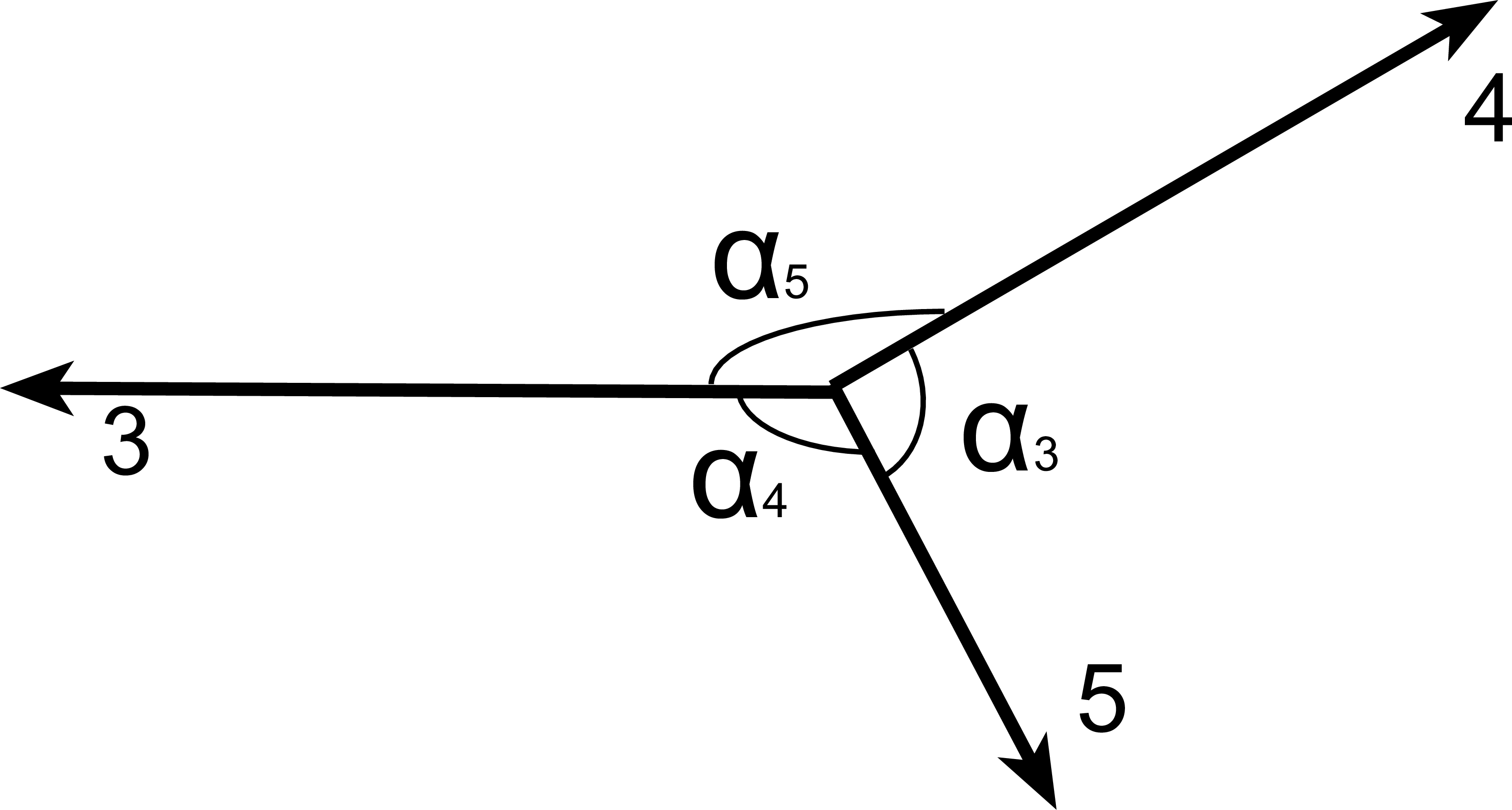
png pdf	Figure 1: Illustration of the three-jet variables in the process 1+2$\to $3+4+5. The scaled energies are related to the angles ($\alpha _i$) among the jets for massless parton.
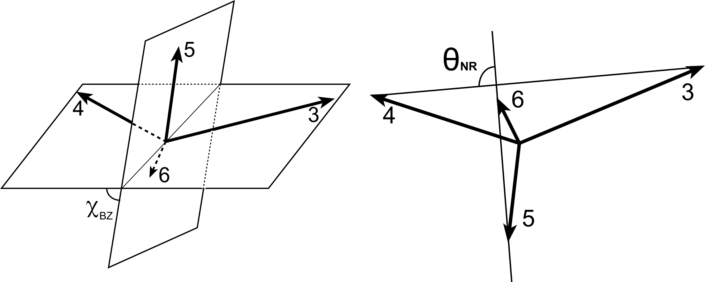
png pdf	Figure 2: Illustration of the Bengtsson-Zerwas angle ($ {\chi _{\mathrm {BZ}}} $) and the Nachtmann-Reiter angle ($ {\theta _{\mathrm {NR}}} $) definitions for the four-jet events. The left figure shows the Bengtsson-Zerwas angle, which is the angle between the plane containing the two leading jets and the plane containing the two nonleading jets. The right figure shows the Nachtmann-Reiter angle, which is the angle between the momentum vector differences of the two leading jets and the two nonleading jets.
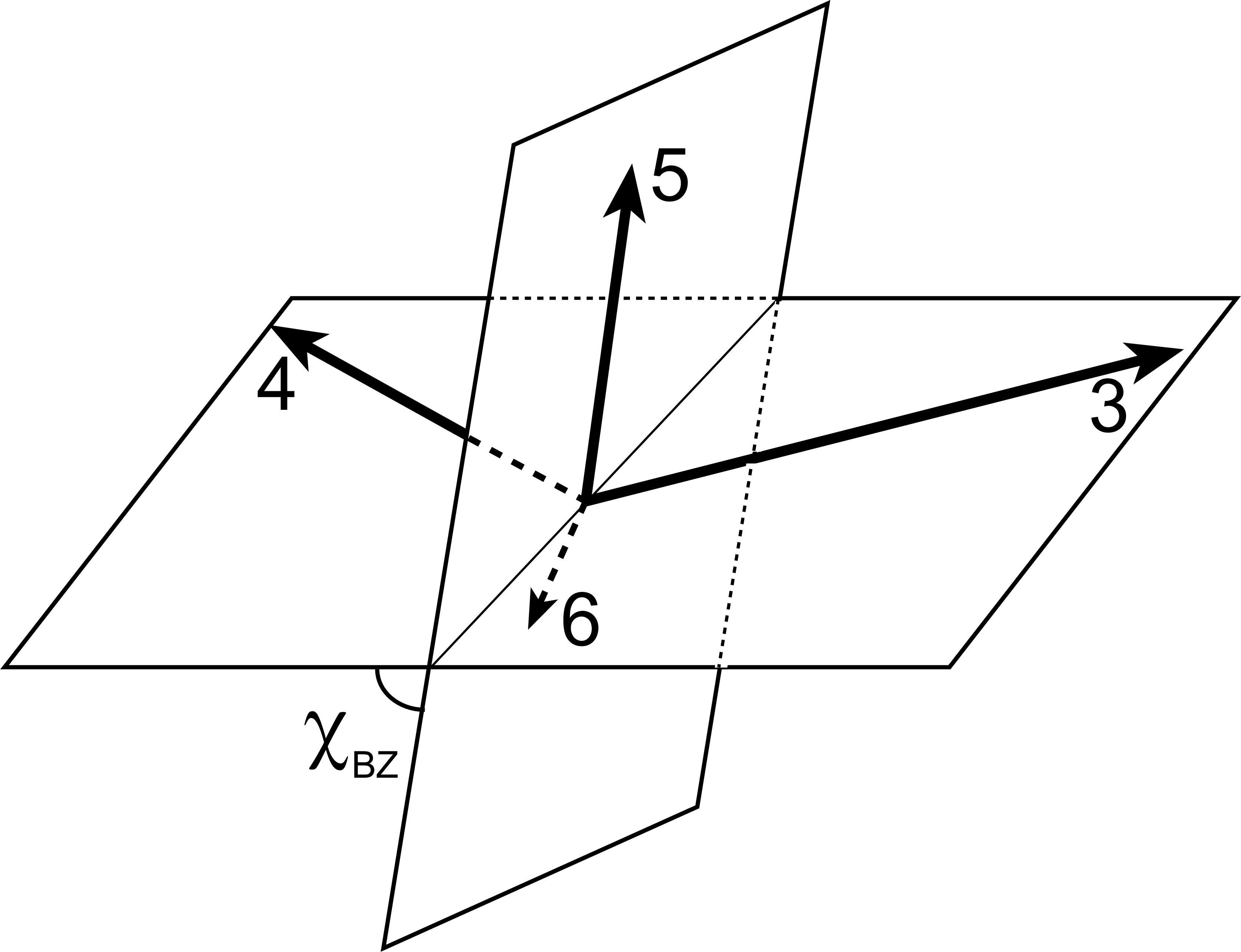
png pdf	Figure 2-a: Illustration of the Bengtsson-Zerwas angle ($ {\chi _{\mathrm {BZ}}} $) and the Nachtmann-Reiter angle ($ {\theta _{\mathrm {NR}}} $) definitions for the four-jet events. The left figure shows the Bengtsson-Zerwas angle, which is the angle between the plane containing the two leading jets and the plane containing the two nonleading jets. The right figure shows the Nachtmann-Reiter angle, which is the angle between the momentum vector differences of the two leading jets and the two nonleading jets.
png pdf	Figure 2-b: Illustration of the Bengtsson-Zerwas angle ($ {\chi _{\mathrm {BZ}}} $) and the Nachtmann-Reiter angle ($ {\theta _{\mathrm {NR}}} $) definitions for the four-jet events. The left figure shows the Bengtsson-Zerwas angle, which is the angle between the plane containing the two leading jets and the plane containing the two nonleading jets. The right figure shows the Nachtmann-Reiter angle, which is the angle between the momentum vector differences of the two leading jets and the two nonleading jets.
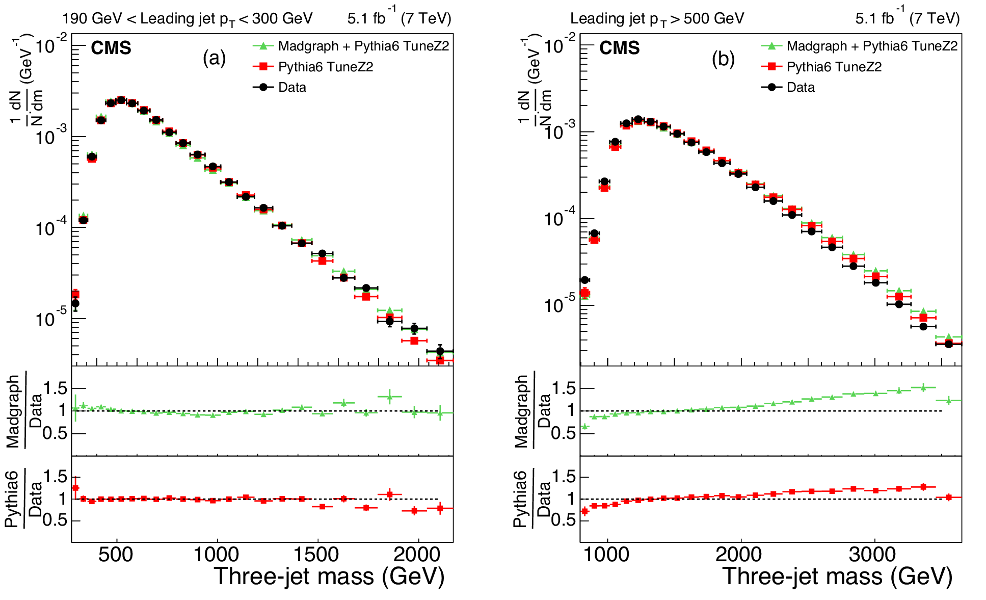
png pdf	Figure 3: The upper panels display the normalized distributions of the reconstructed three-jet mass for events where the most forward jet has $ {\| y \| }<2.5$. Figures differ by $ p_{\mathrm{T}} $ ranges of the leading jet: 190-300 GeV (a), and above 500 GeV (b) for data (before correction due to detector effects) and predictions from MC generators. The bottom panel of each plot shows the ratio of MC predictions to the data. The data are shown with only statistical uncertainty.
png pdf	Figure 3-a: The upper panels display the normalized distributions of the reconstructed three-jet mass for events where the most forward jet has $ {\| y \| }<2.5$. Figures differ by $ p_{\mathrm{T}} $ ranges of the leading jet: 190-300 GeV (a), and above 500 GeV (b) for data (before correction due to detector effects) and predictions from MC generators. The bottom panel of each plot shows the ratio of MC predictions to the data. The data are shown with only statistical uncertainty.-a
png pdf	Figure 3-b: The upper panels display the normalized distributions of the reconstructed three-jet mass for events where the most forward jet has $ {\| y \| }<2.5$. Figures differ by $ p_{\mathrm{T}} $ ranges of the leading jet: 190-300 GeV (a), and above 500 GeV (b) for data (before correction due to detector effects) and predictions from MC generators. The bottom panel of each plot shows the ratio of MC predictions to the data. The data are shown with only statistical uncertainty.-b
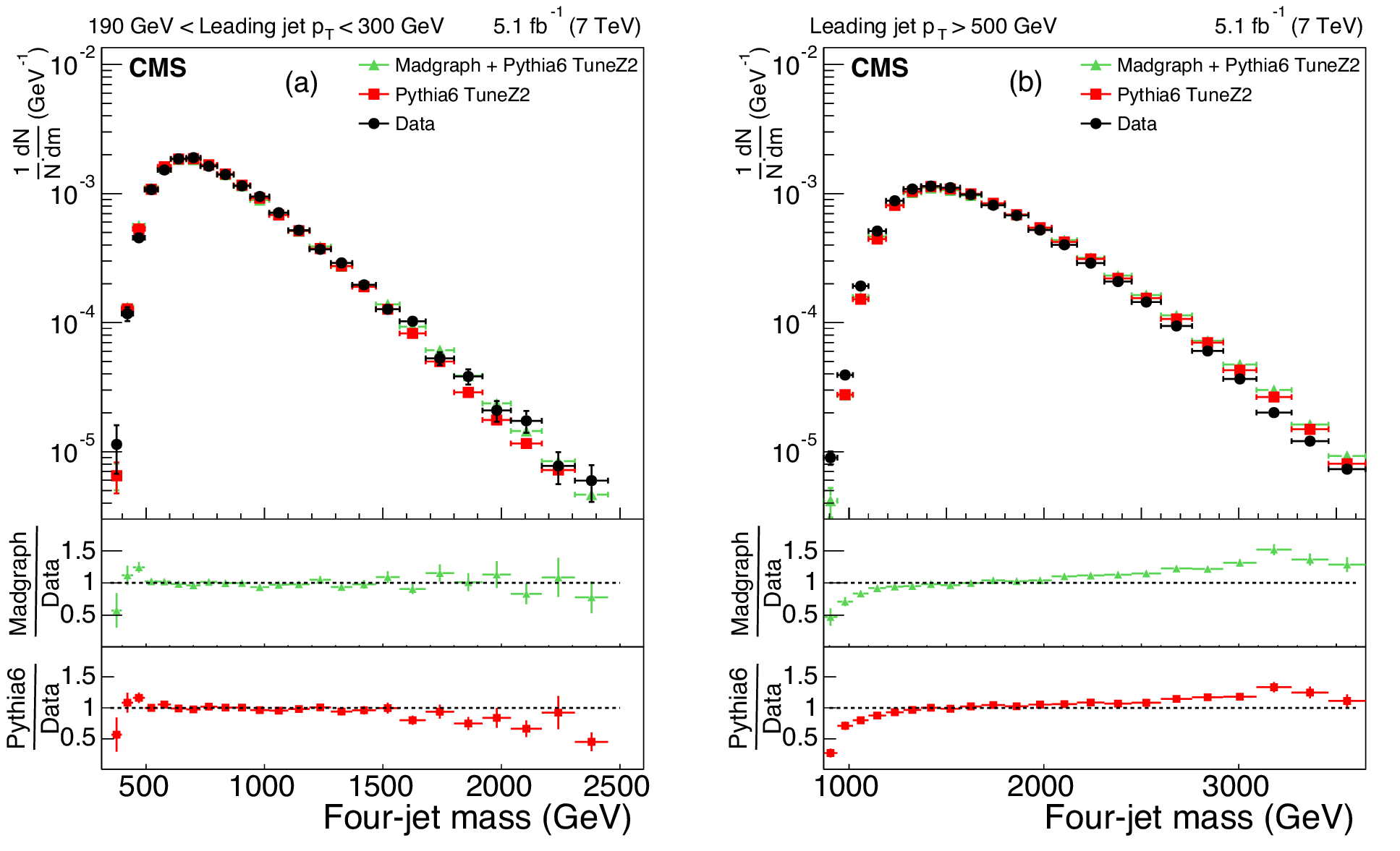
png pdf	Figure 4: The upper panels display the normalized distributions of the reconstructed four-jet mass for events where the most forward jet has $ {\| y \| }< 2.5$. The other explanations are the same as Fig. 3.
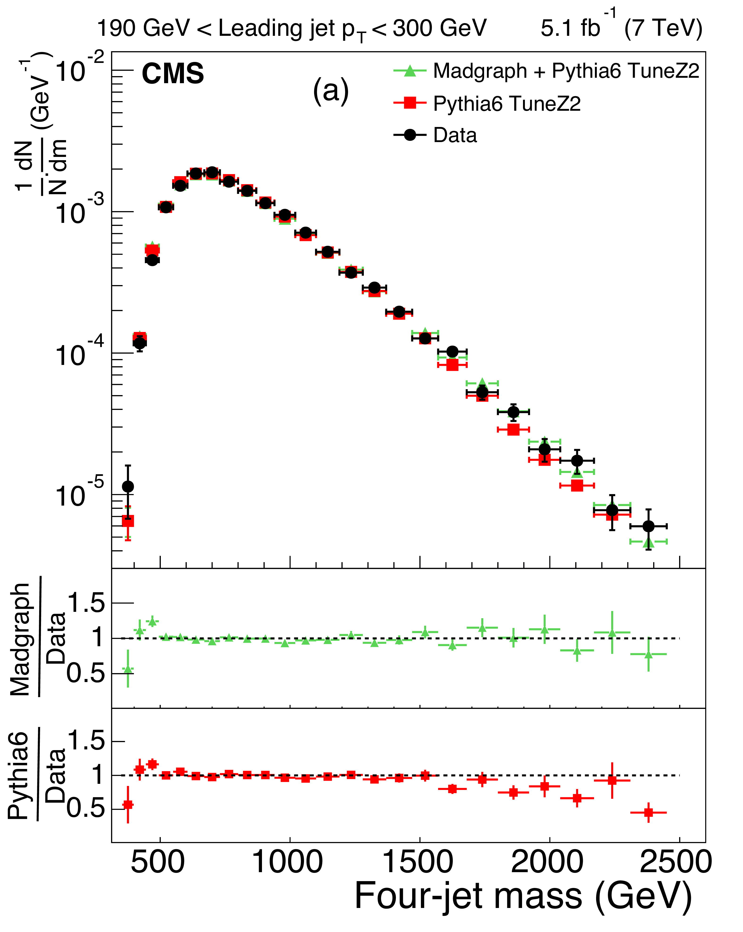
png pdf	Figure 4-a: The upper panels display the normalized distributions of the reconstructed four-jet mass for events where the most forward jet has $ {\| y \| }< 2.5$. The other explanations are the same as Fig. 3.
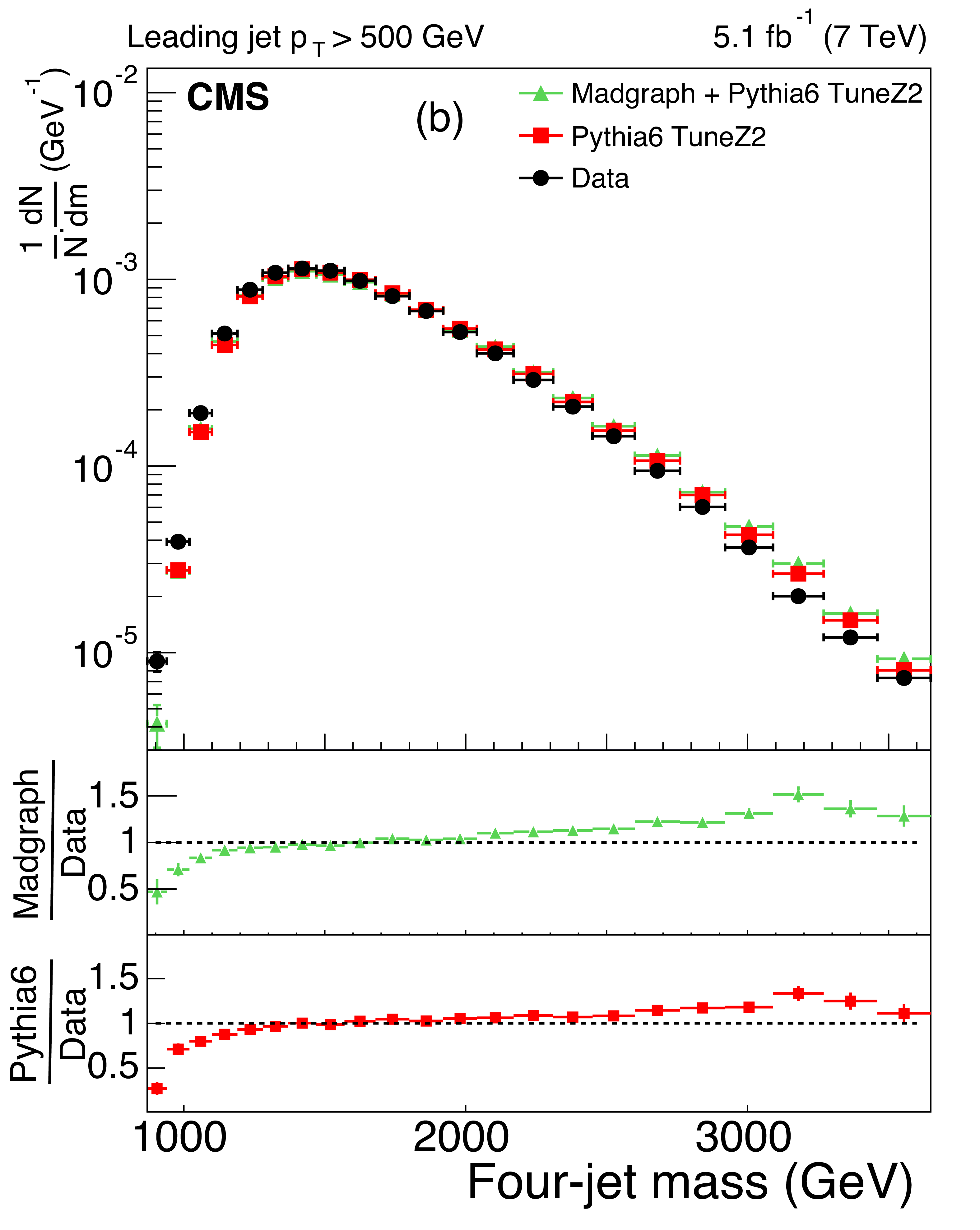
png pdf	Figure 4-b: The upper panels display the normalized distributions of the reconstructed four-jet mass for events where the most forward jet has $ {\| y \| }< 2.5$. The other explanations are the same as Fig. 3.
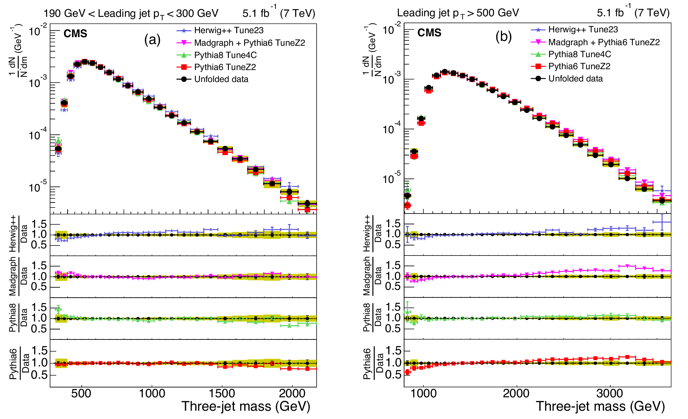
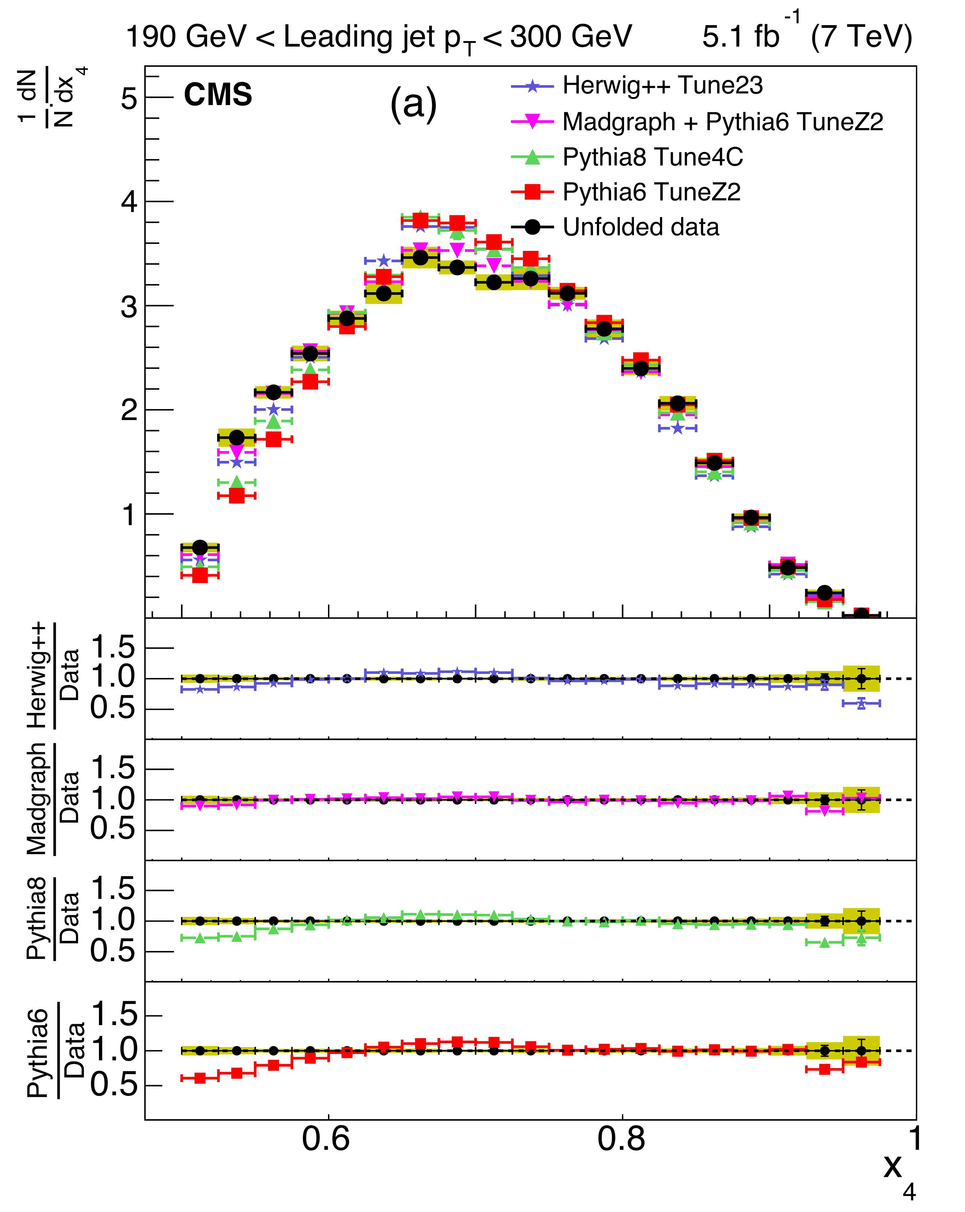
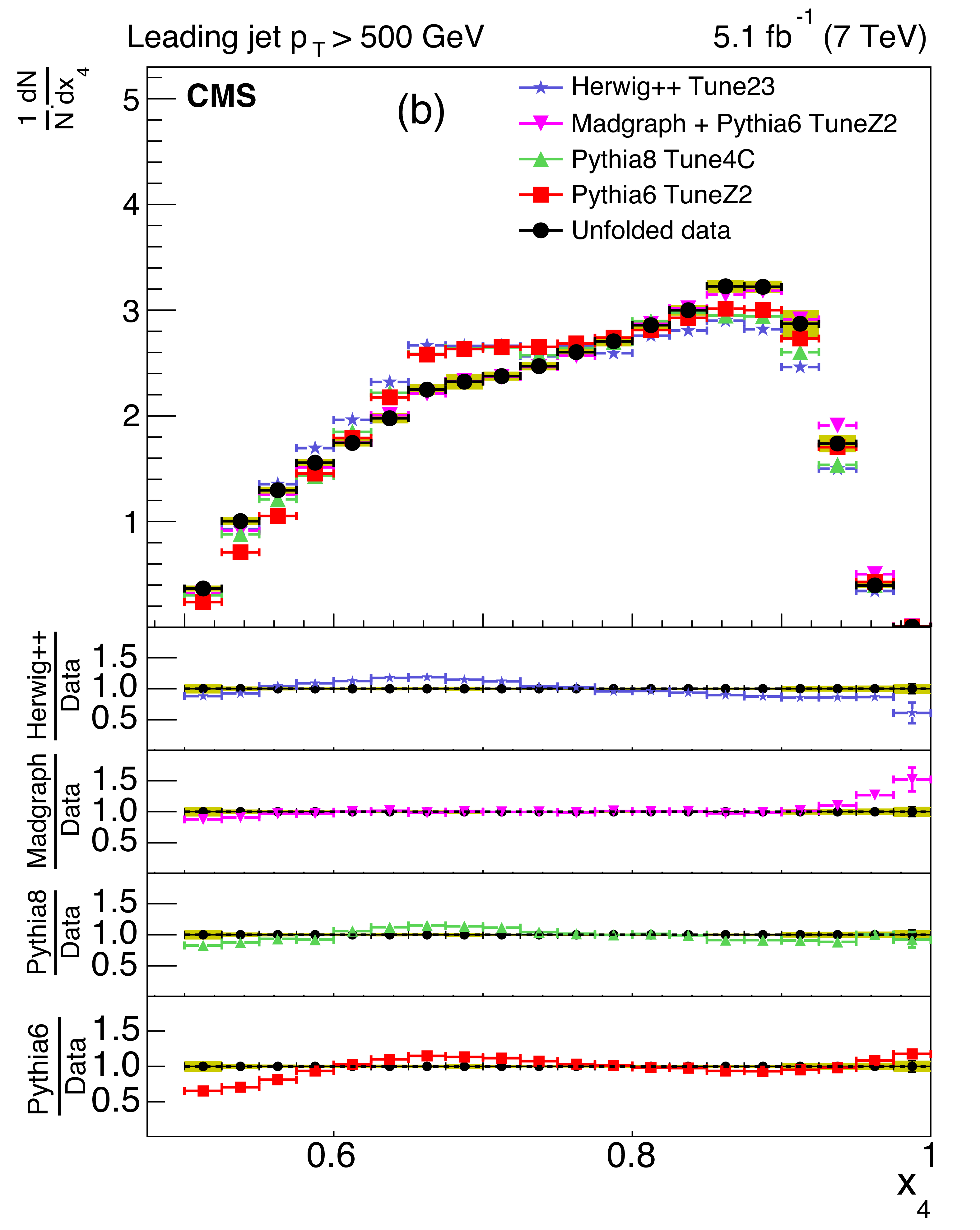
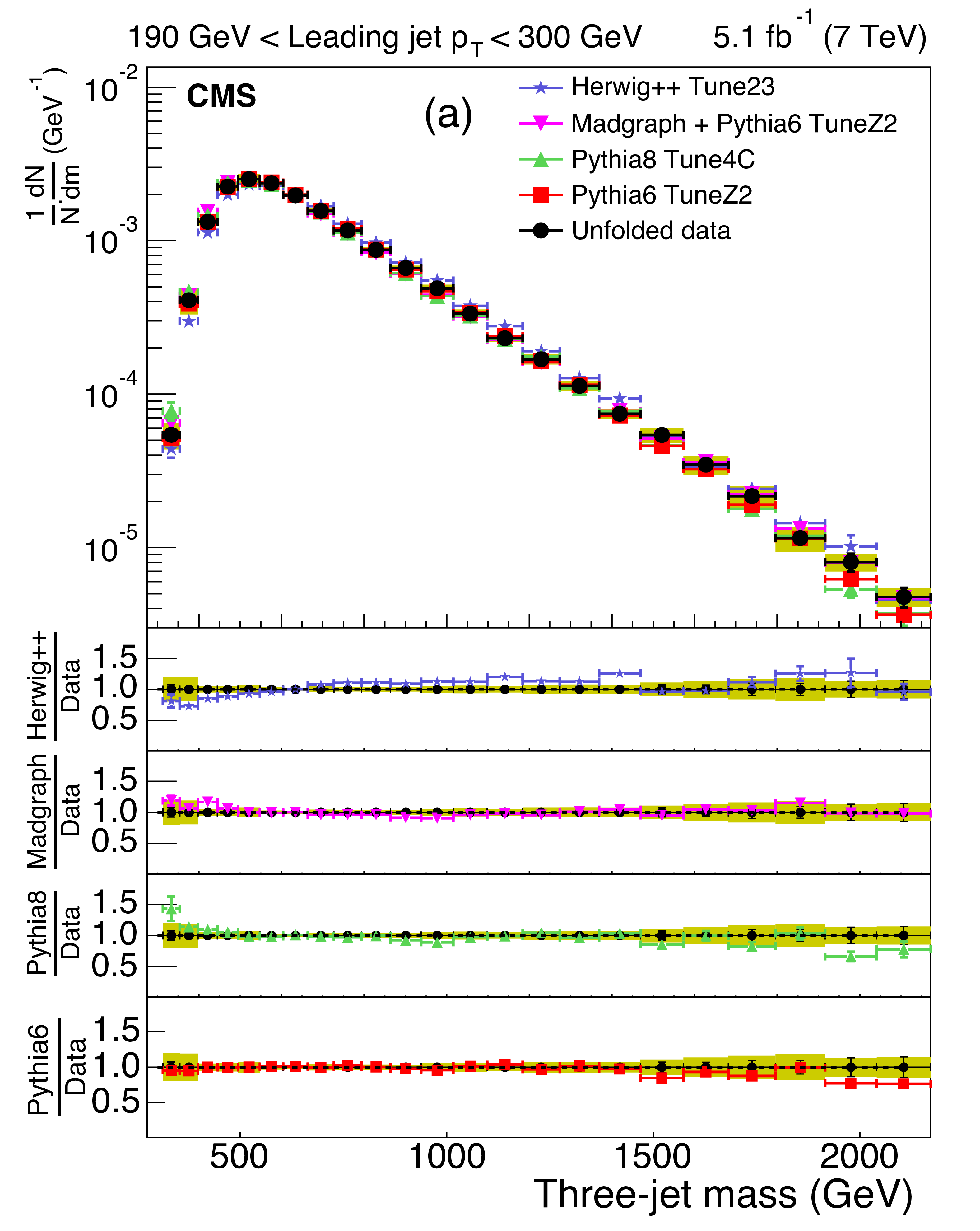
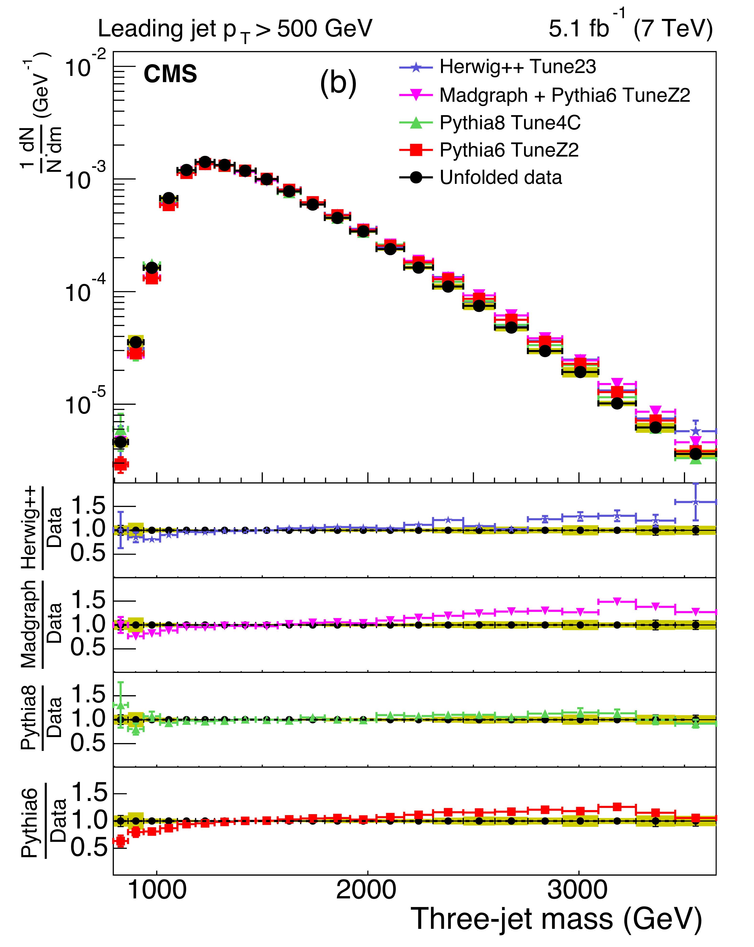
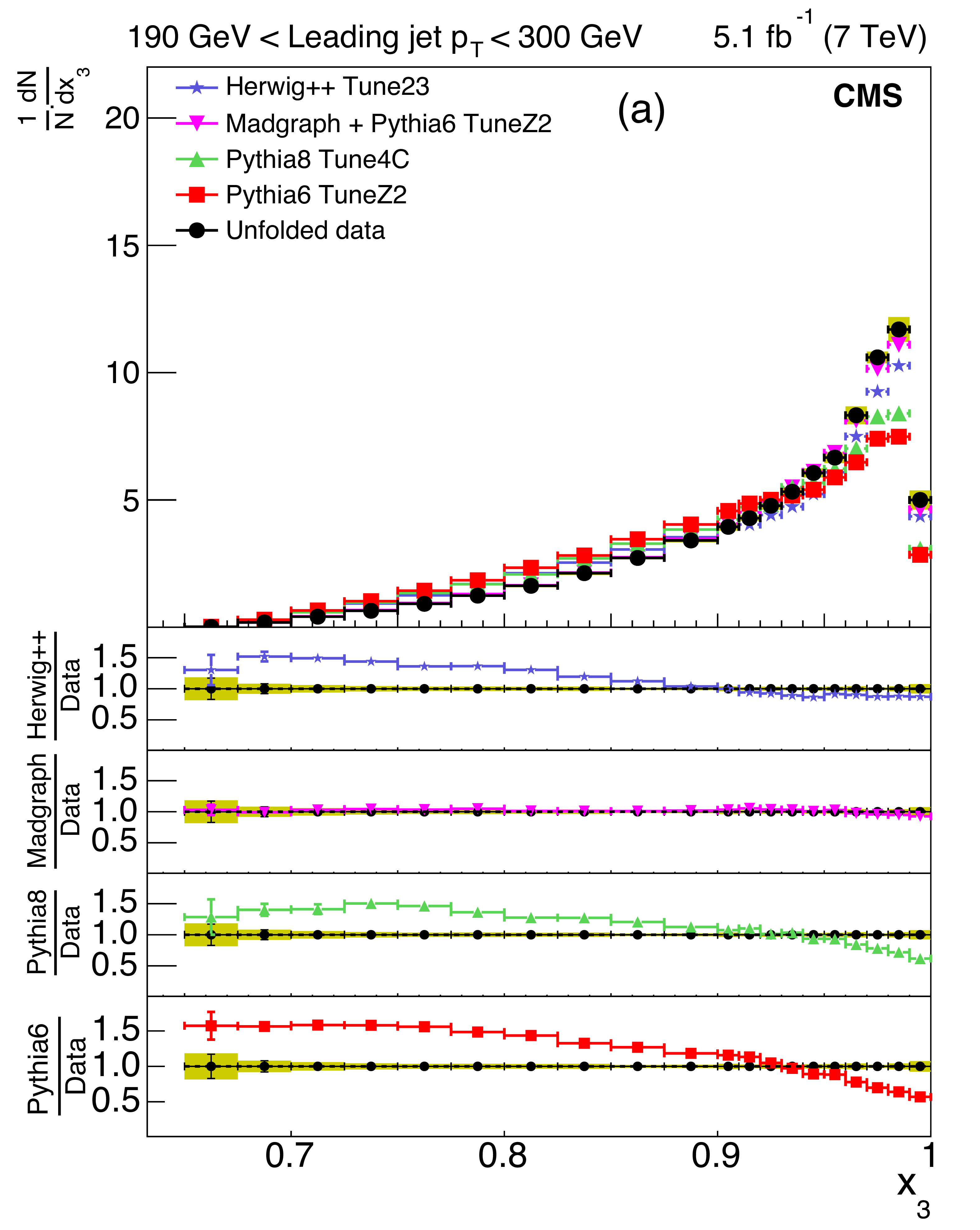
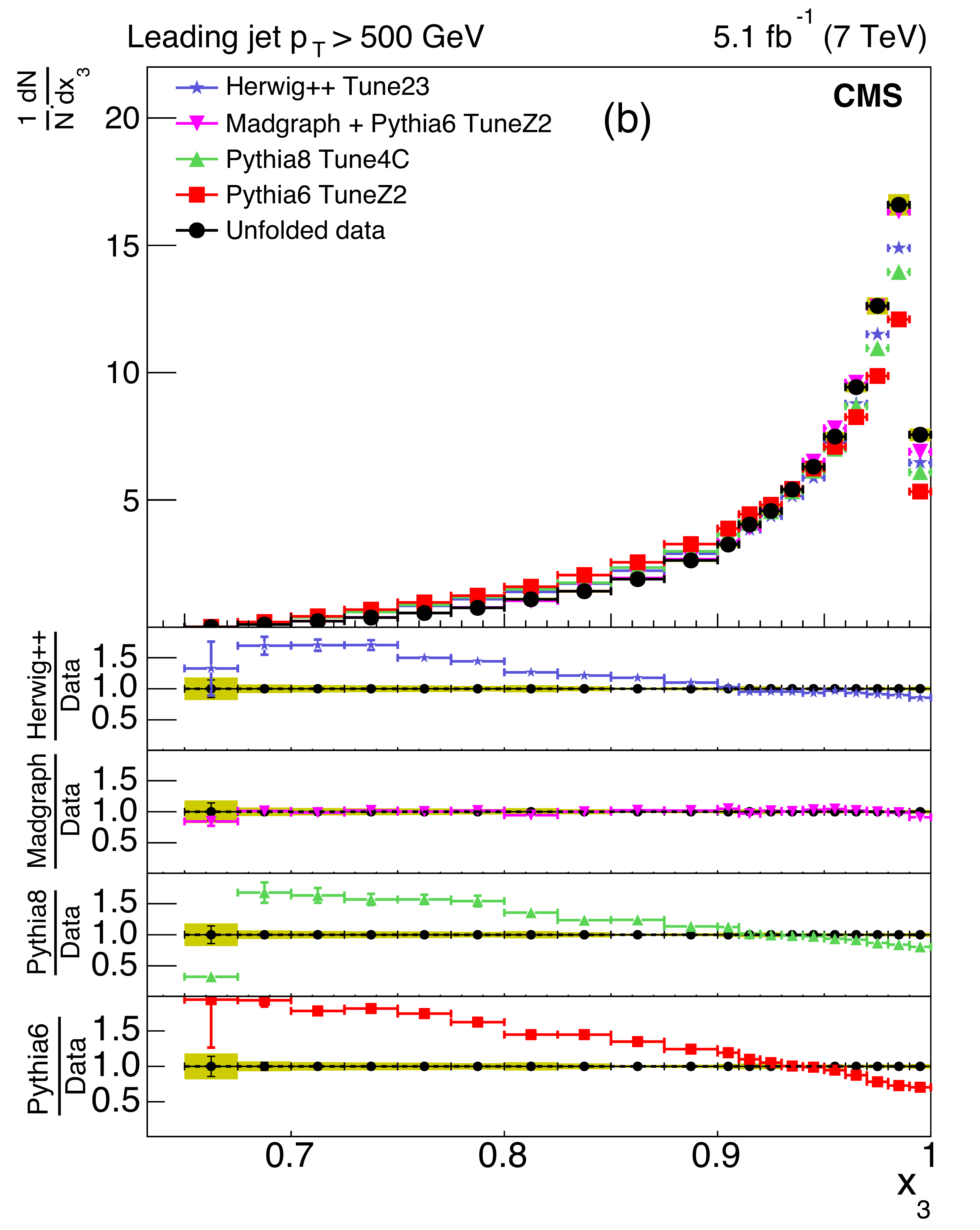
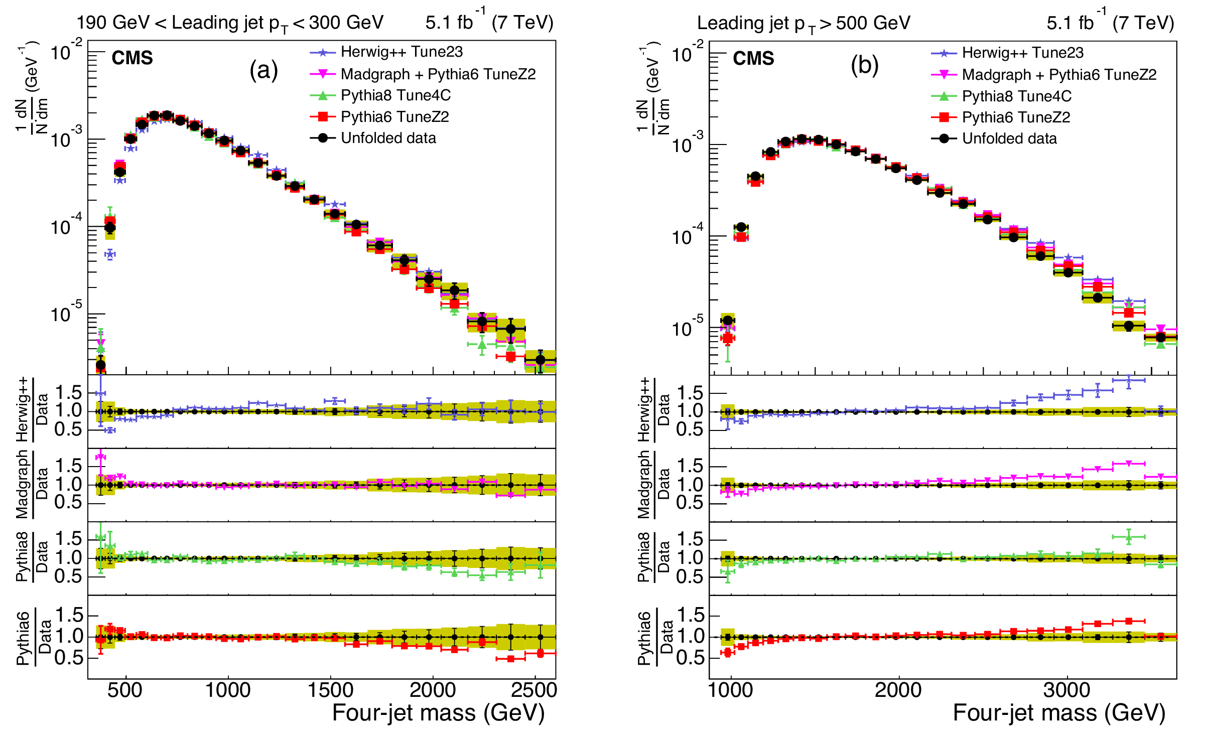
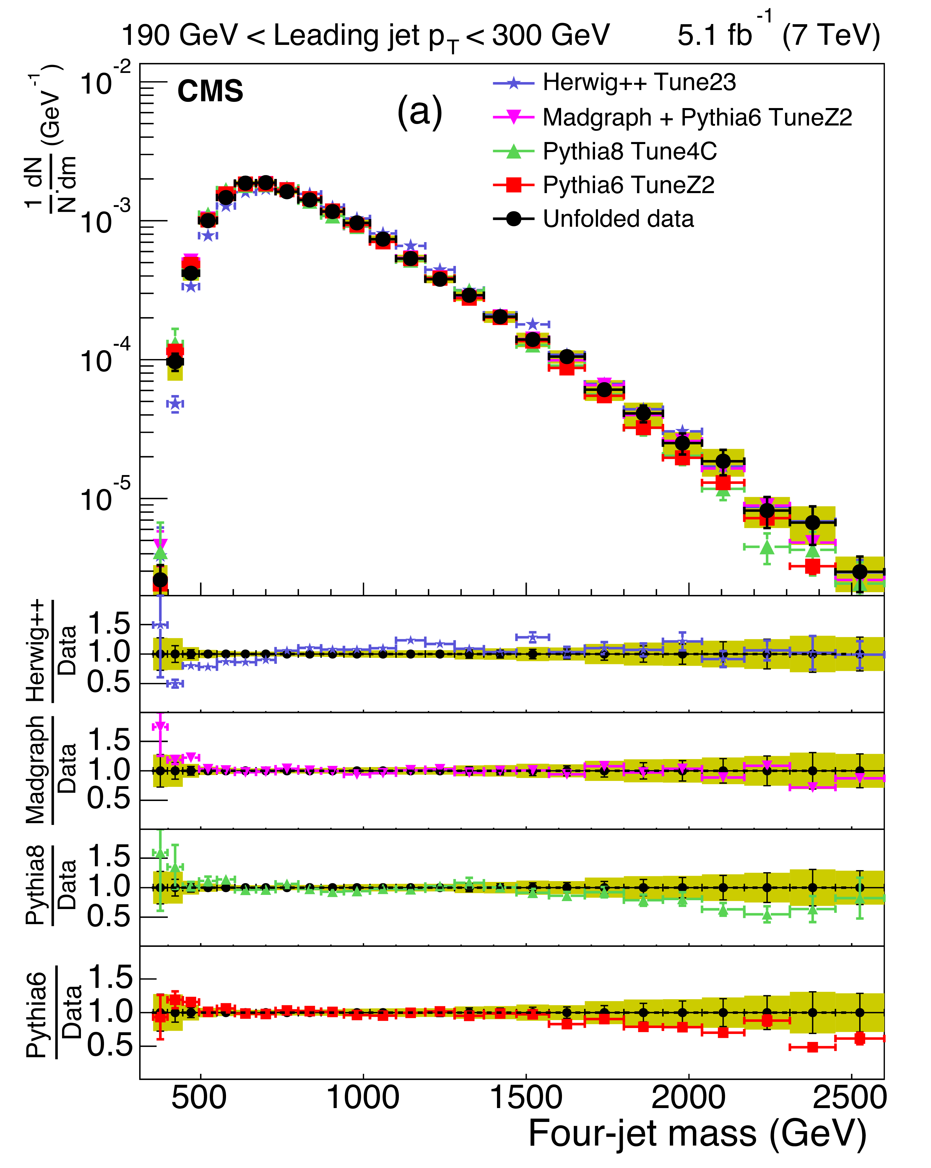
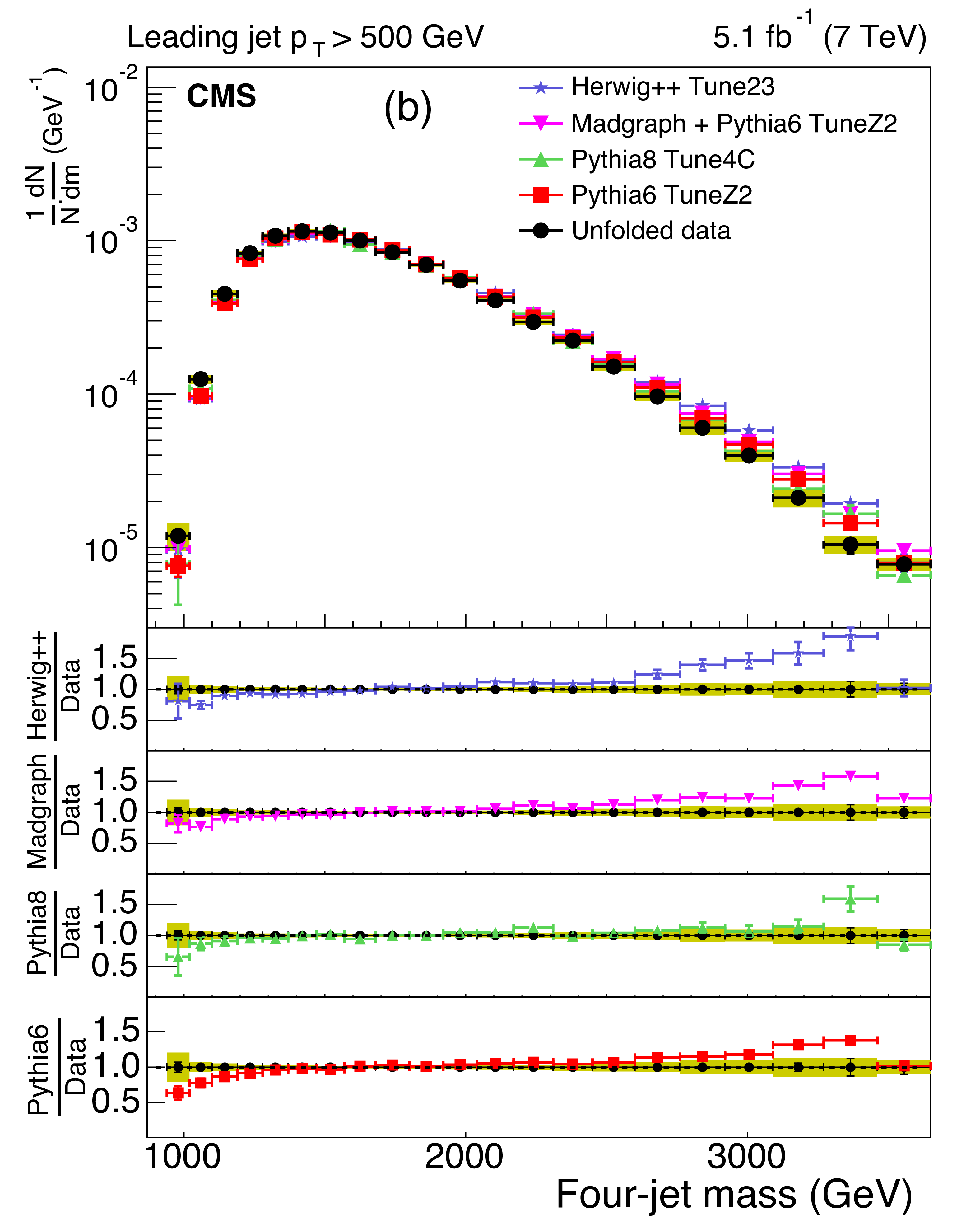
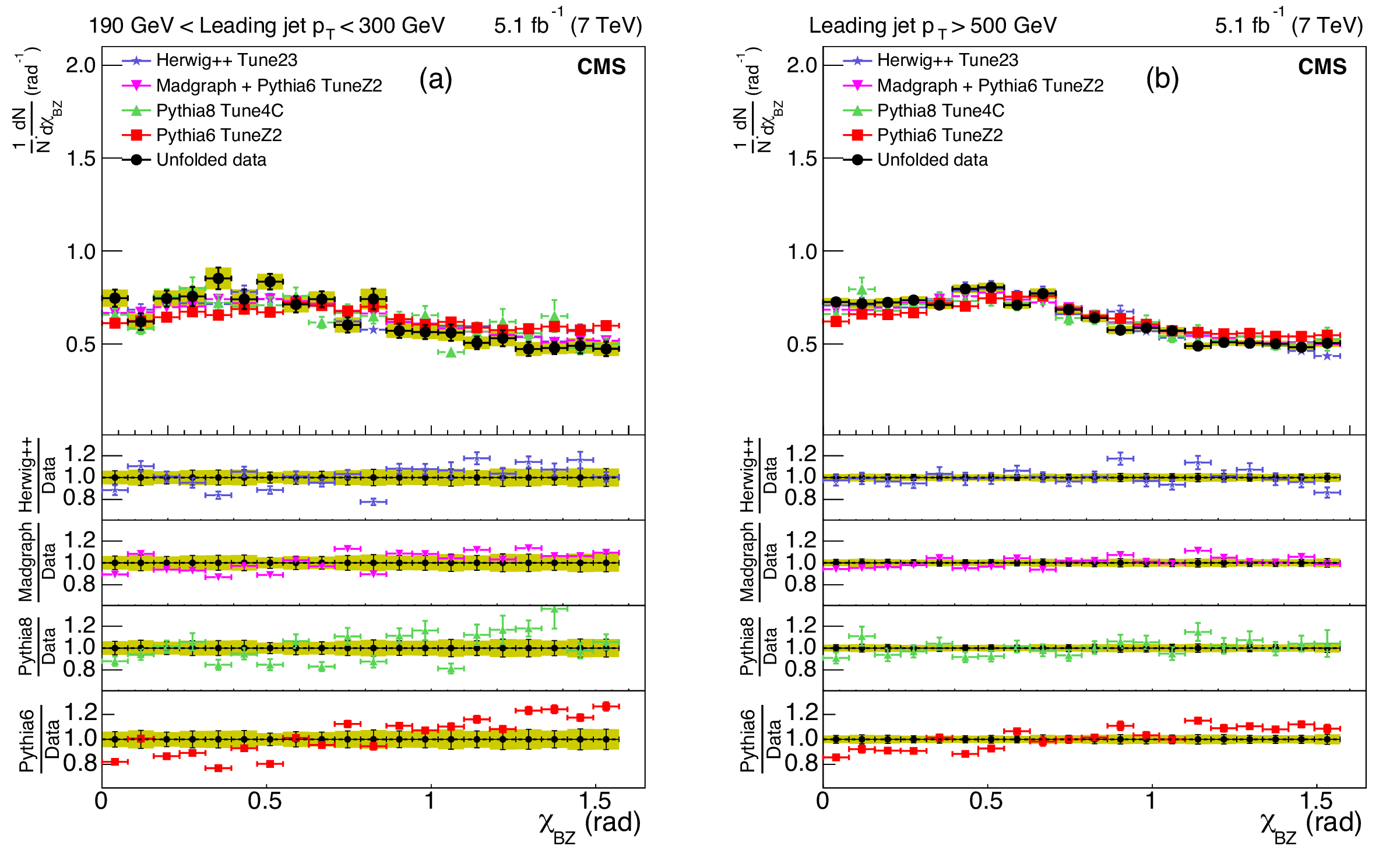
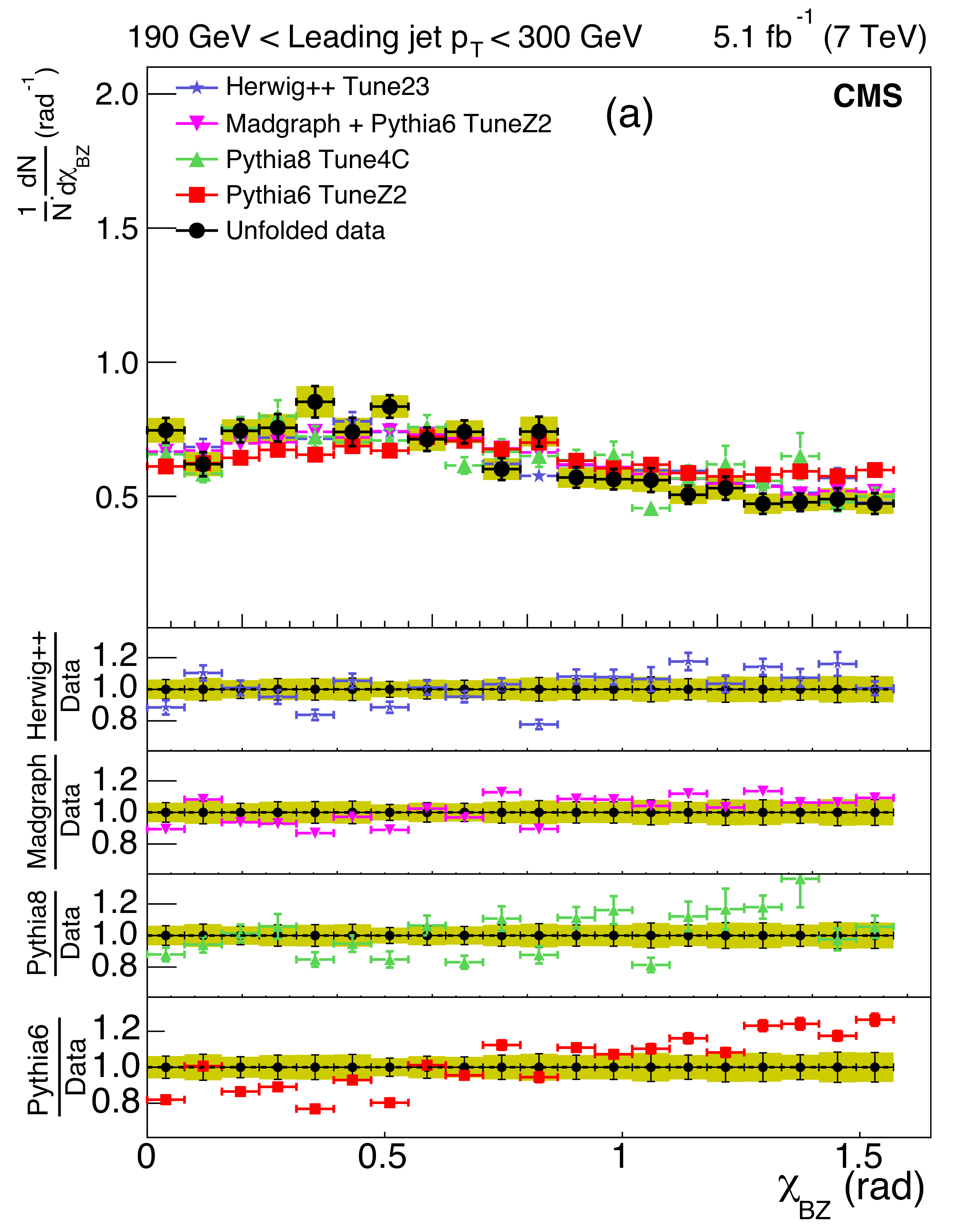
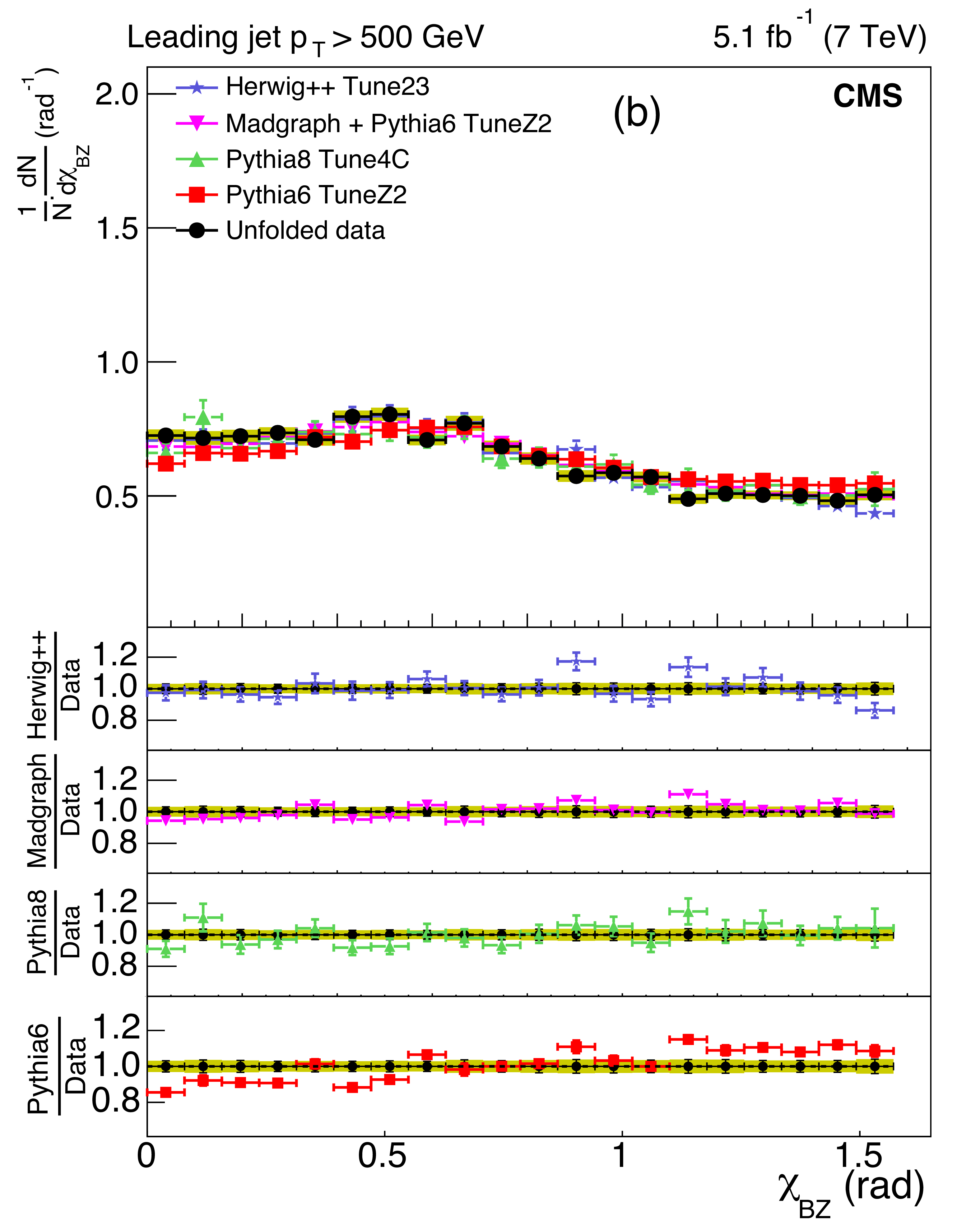
png pdf	Figure 5: Distribution of the three-jet mass superposed with predictions from four MC models: {pythia} {6}, {pythia} {8}, MadGraph {+}{pythia} {6} , {herwig++} . The distributions are obtained from inclusive three-jet sample with the jets restricted in the $ {\| y \| }$ region $0.0 < {\| y \| }< 2.5$, and with leading-jet $ p_{\mathrm{T}} $ between 190 and 300 GeV (a) or above 500 GeV (b). The data points are shown with statistical uncertainty only and the bands indicate the statistical and systematic uncertainties combined in quadrature. The lower panels of each plot show the ratios of MC predictions to the data. The ratios are shown with statistical uncertainty in the data as well as in the MC, while the band shows combined statistical and systematic uncertainties.
png pdf	Figure 5-a: Distribution of the three-jet mass superposed with predictions from four MC models: {pythia} {6}, {pythia} {8}, MadGraph {+}{pythia} {6} , {herwig++} . The distributions are obtained from inclusive three-jet sample with the jets restricted in the $ {\| y \| }$ region $0.0 < {\| y \| }< 2.5$, and with leading-jet $ p_{\mathrm{T}} $ between 190 and 300 GeV (a) or above 500 GeV (b). The data points are shown with statistical uncertainty only and the bands indicate the statistical and systematic uncertainties combined in quadrature. The lower panels of each plot show the ratios of MC predictions to the data. The ratios are shown with statistical uncertainty in the data as well as in the MC, while the band shows combined statistical and systematic uncertainties.
png pdf	Figure 5-b: Distribution of the three-jet mass superposed with predictions from four MC models: {pythia} {6}, {pythia} {8}, MadGraph {+}{pythia} {6} , {herwig++} . The distributions are obtained from inclusive three-jet sample with the jets restricted in the $ {\| y \| }$ region $0.0 < {\| y \| }< 2.5$, and with leading-jet $ p_{\mathrm{T}} $ between 190 and 300 GeV (a) or above 500 GeV (b). The data points are shown with statistical uncertainty only and the bands indicate the statistical and systematic uncertainties combined in quadrature. The lower panels of each plot show the ratios of MC predictions to the data. The ratios are shown with statistical uncertainty in the data as well as in the MC, while the band shows combined statistical and systematic uncertainties.
png pdf	Figure 6: Corrected normalized distribution of scaled energy of the leading-jet in the inclusive three-jet sample. The other explanations are the same as Fig. 5.
png pdf	Figure 6-a: Corrected normalized distribution of scaled energy of the leading-jet in the inclusive three-jet sample. The other explanations are the same as Fig. 5.
png pdf	Figure 6-b: Corrected normalized distribution of scaled energy of the leading-jet in the inclusive three-jet sample. The other explanations are the same as Fig. 5.
png pdf	Figure 7: Corrected normalized distribution of scaled energy of the second-leading jet in the inclusive three-jet sample. The other explanations are the same as Fig. 5.
png pdf	Figure 7-a: Corrected normalized distribution of scaled energy of the second-leading jet in the inclusive three-jet sample. The other explanations are the same as Fig. 5.
png pdf	Figure 7-b: Corrected normalized distribution of scaled energy of the second-leading jet in the inclusive three-jet sample. The other explanations are the same as Fig. 5.
png pdf	Figure 8: Corrected normalized distribution of four-jet mass. The other explanations are the same as Fig. 5.
png pdf	Figure 8-a: Corrected normalized distribution of four-jet mass. The other explanations are the same as Fig. 5.
png pdf	Figure 8-b: Corrected normalized distribution of four-jet mass. The other explanations are the same as Fig. 5.
png pdf	Figure 9: Corrected normalized distribution of the Bengtsson-Zerwas angle. The other explanations are the same as Fig. 5.
png pdf	Figure 9-a: Corrected normalized distribution of the Bengtsson-Zerwas angle. The other explanations are the same as Fig. 5.
png pdf	Figure 9-b: Corrected normalized distribution of the Bengtsson-Zerwas angle. The other explanations are the same as Fig. 5.
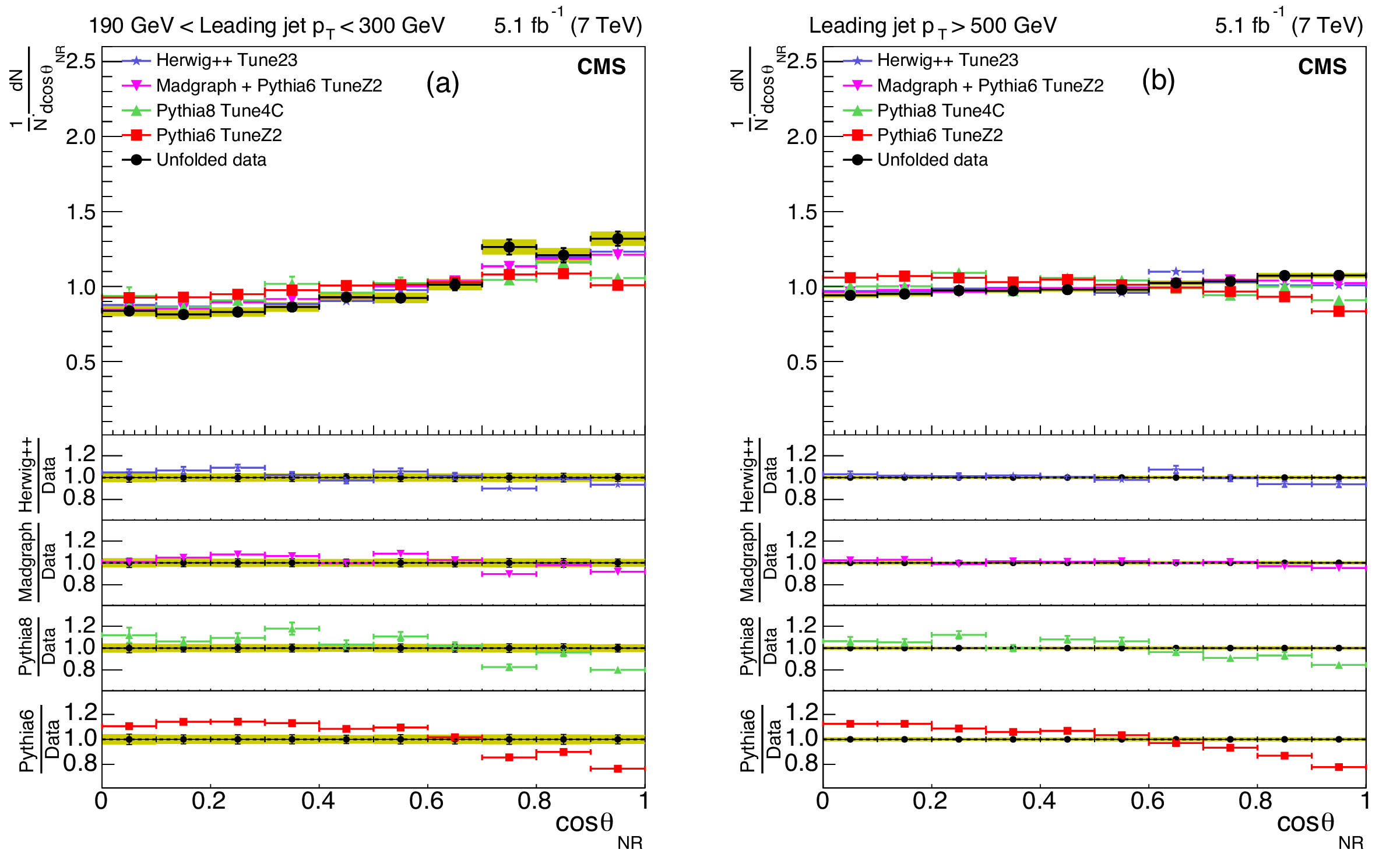
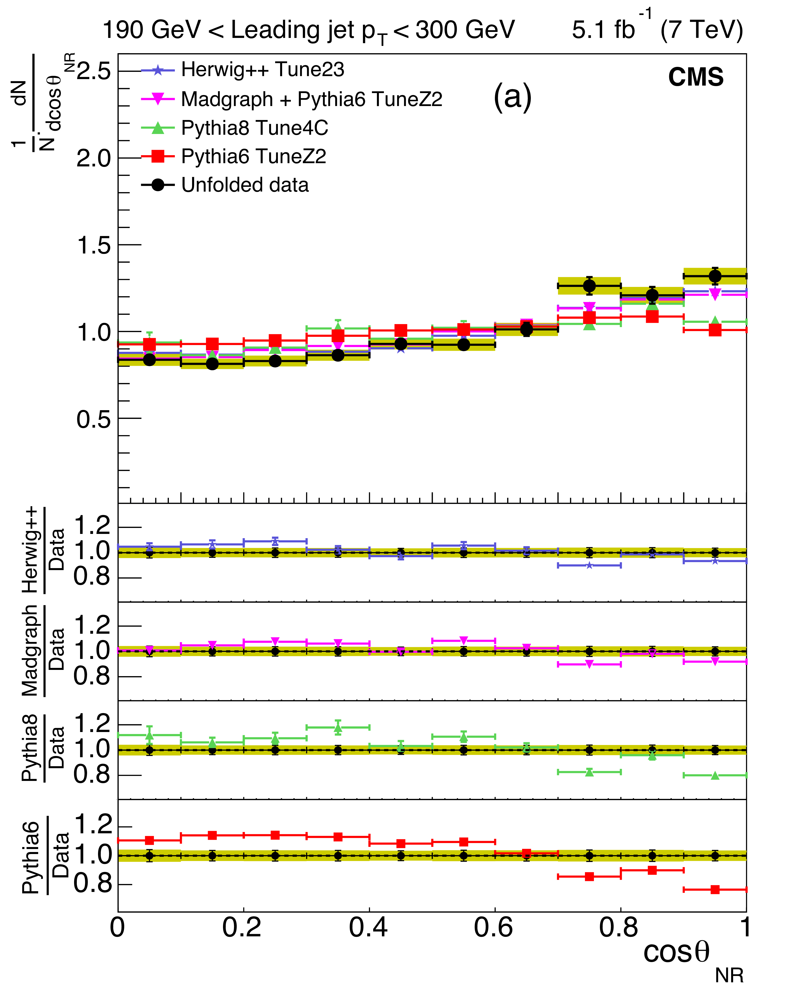
png pdf	Figure 10: Corrected normalized distribution of the cosine of the Nachtmann-Reiter angle. The other explanations are the same as Fig. 5.
png pdf	Figure 10-a: Corrected normalized distribution of the cosine of the Nachtmann-Reiter angle. The other explanations are the same as Fig. 5.
png pdf	Figure 10-b: Corrected normalized distribution of the cosine of the Nachtmann-Reiter angle. The other explanations are the same as Fig. 5.

Tables
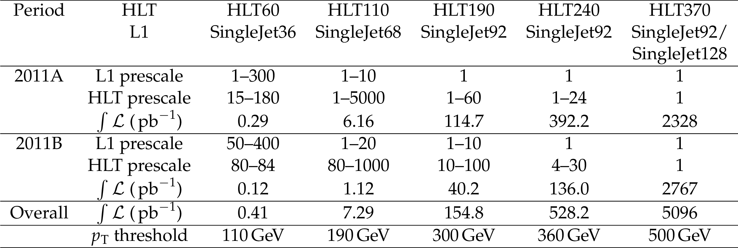
png pdf	Table 1: Prescales, integrated luminosity and offline $ p_{\mathrm{T}} $ threshold of the leading jet for different trigger paths. The terminology for Level 1 (L1) triggers as well as HLT includes the jet $ p_{\mathrm{T}} $ threshold (in GeV) applicable to the trigger.
png pdf	Table 2: Threshold of the leading jet $ p_{\mathrm{T}} $ for different HLT paths. This paper shows results from two representative trigger paths HLT110 and HLT370.
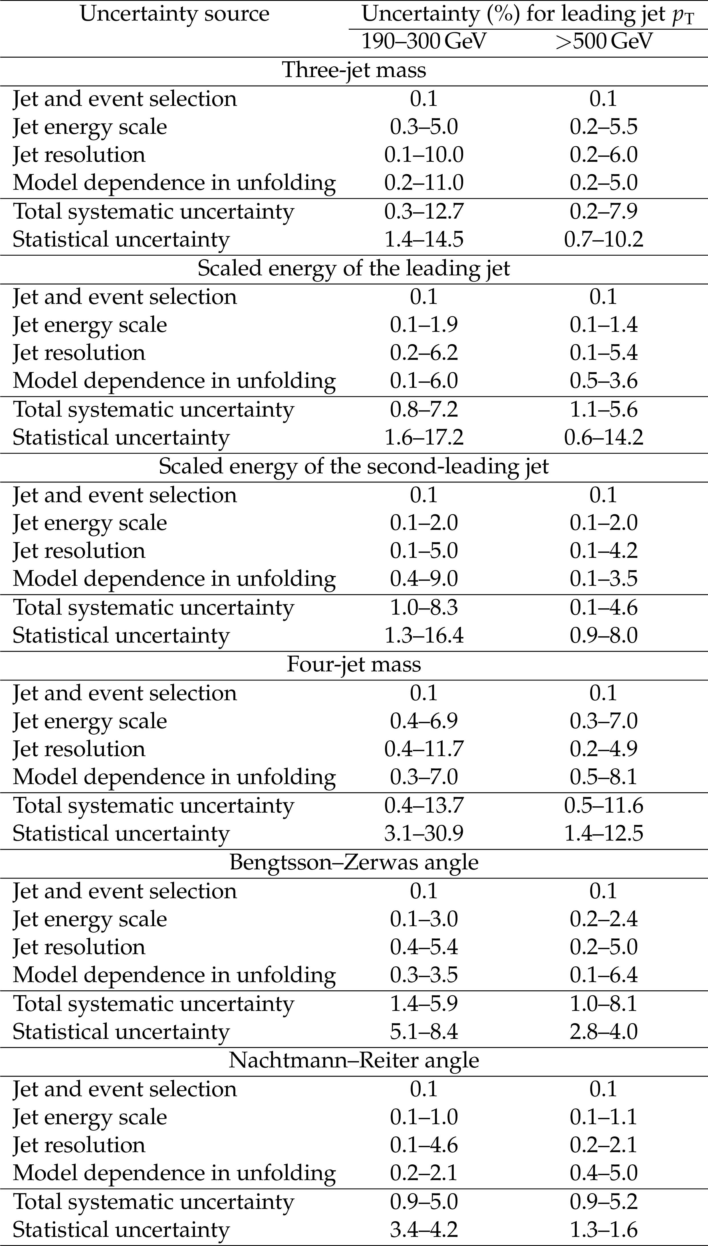
png pdf	Table 3: Uncertainty ranges among the different bins in the topological distributions of the three- and four-jet variables.

Summary

Distributions of topological variables for inclusive three- and four-jet events in pp collisions measured with the CMS detector at a centre-of-mass energy of 7 TeV were presented using a data sample corresponding to an integrated luminosity of 5.1 fb$^{-1}$. The distributions were corrected for detector effects, and systematic uncertainties were estimated. These corrected distributions were compared with the predictions from four LO MC models: PYTHIA-6, PYTHIA-8, HERWIG++, and MadGraph+PYTHIA-6. Distributions of three- and four-jet invariant mass from all models show significant deviation from the data at high mass. The fact that all models have a common PDF suggests that the PDF errors at high mass are underestimated. The PDFs at high invariant mass have recently been constrained by CMS using dijet $ p_{\mathrm{T}} $ distributions [44]. The MadGraph simulations are based on tree-level calculations for two-, three-, and four-parton final states, while PYTHIA and HERWIG++ can have only two partons in the final state before showering. Not surprisingly, the three-jet predictions of MadGraph+PYTHIA-6 give a more consistent description of the distributions studied in this analysis. The notable exception is at high $x_4$ (the next-to-leading jet), where two jets carry most of the CM energy. The difference is probably due to a double counting of three-parton with two-parton (with a parton from showering) final states. The PYTHIA and HERWIG++ models give poor descriptions of the energy fractions in the three-jet final state. In particular, the distributions of $x_3$ (the leading jet) show large shape differences between data and theory that are inconsistent with PDFs or hadronization model uncertainties. Since the distributions from MadGraph+PYTHIA-6 agree with those from the data, the discrepancies with PYTHIA and HERWIG++ are likely due to missing higher multiplicity ME, which are present in MadGraph. All the models compared in this study do remarkably well describing the four-jet Bengtsson-Zerwas angle. The PYTHIA models have some systematic deviation from the data in describing the Nachtmann-Reiter angle. Parton showers with angular ordering, as implemented in HERWIG++, yield a better agreement with the measured data for these angular variables.