CMS-SMP-13-002

CMS-SMP-13-002 ; CERN-PH-EP-2014-068
Measurement of the ratio of inclusive jet cross sections using the anti-$ k_{\mathrm{T}} $ algorithm with radius parameters R = 0.5 and 0.7 in pp collisions at $\sqrt{s}$ = 7 TeV
CMS Collaboration
2 June 2014
Phys. Rev. D 90 (2014) 072006
Abstract: Measurements of the inclusive jet cross section with the anti-$k_t$ clustering algorithm are presented for two radius parameters, R=0.5 and 0.7. They are based on data from LHC proton-proton collisions at $\sqrt{s}$ = 7 TeV corresponding to an integrated luminosity of 5.0 inverse-femtobarns collected with the CMS detector in 2011. The ratio of these two measurements is obtained as a function of the rapidity and transverse momentum of the jets. Significant discrepancies are found comparing the data to leading-order simulations and to fixed-order calculations at next-to-leading order, corrected for nonperturbative effects, whereas simulations with next-to-leading-order matrix elements matched to parton showers describe the data best.
Links: e-print arXiv:1406.0324 [hep-ex] (PDF) ; CDS record ; inSPIRE record ; Public twiki page ; Rivet record ; HepData record ; CADI line (restricted) ;

Figures	CMS Publications

Figures
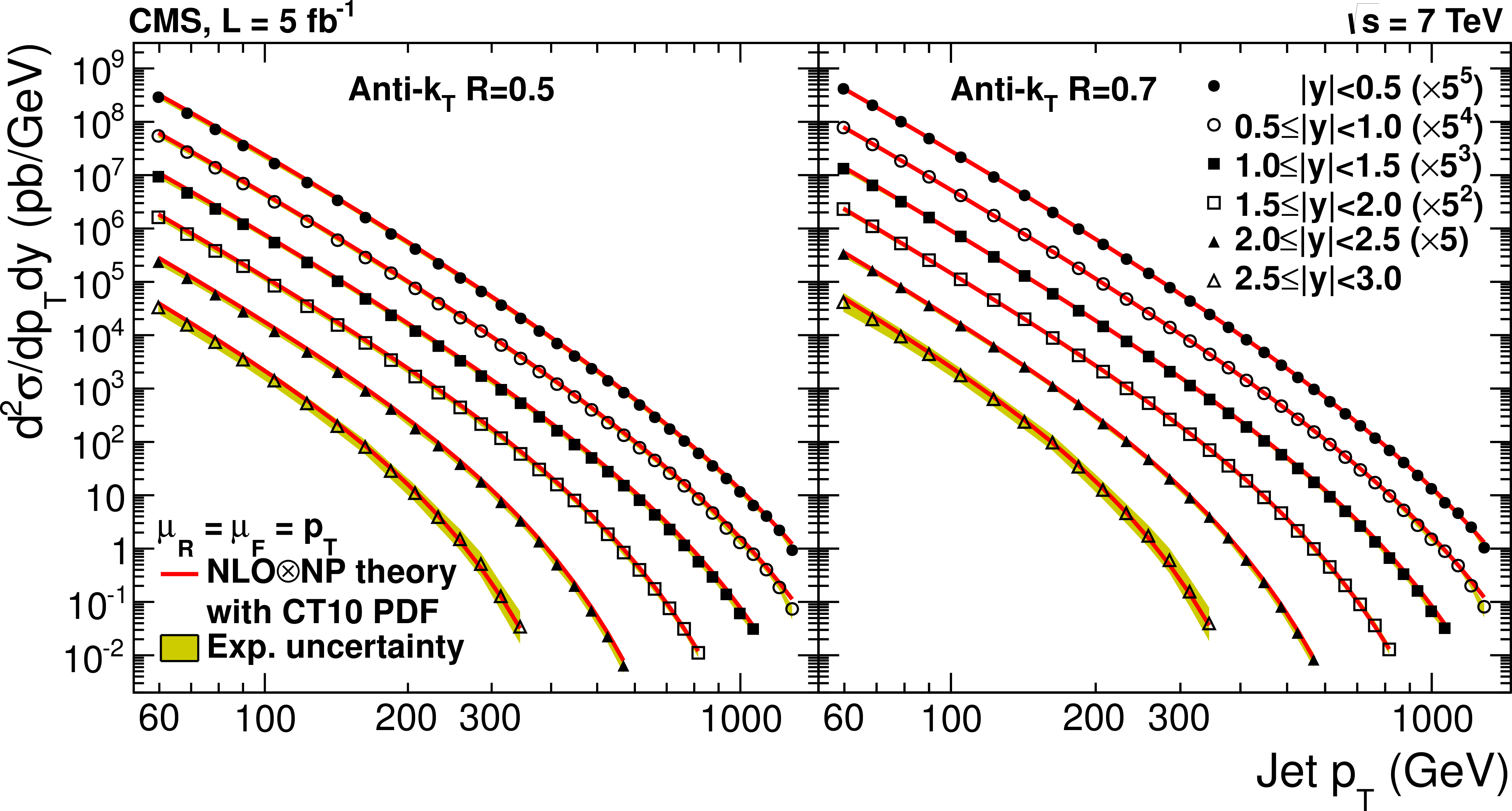
png pdf	Figure 1: Unfolded inclusive jet cross section with anti-$k_{\mathrm{T}}$ R = 0.5 (a) and 0.7 (b) compared to an NLO$\otimes$NP theory prediction using the CT10 NLO PDF set. The renormalization ($\mu_{\mathrm{R}}$) and factorization ($\mu_{\mathrm{F}}$) scales are defined to be the transverse momentum $p_{\mathrm{T}}$ of the jets.
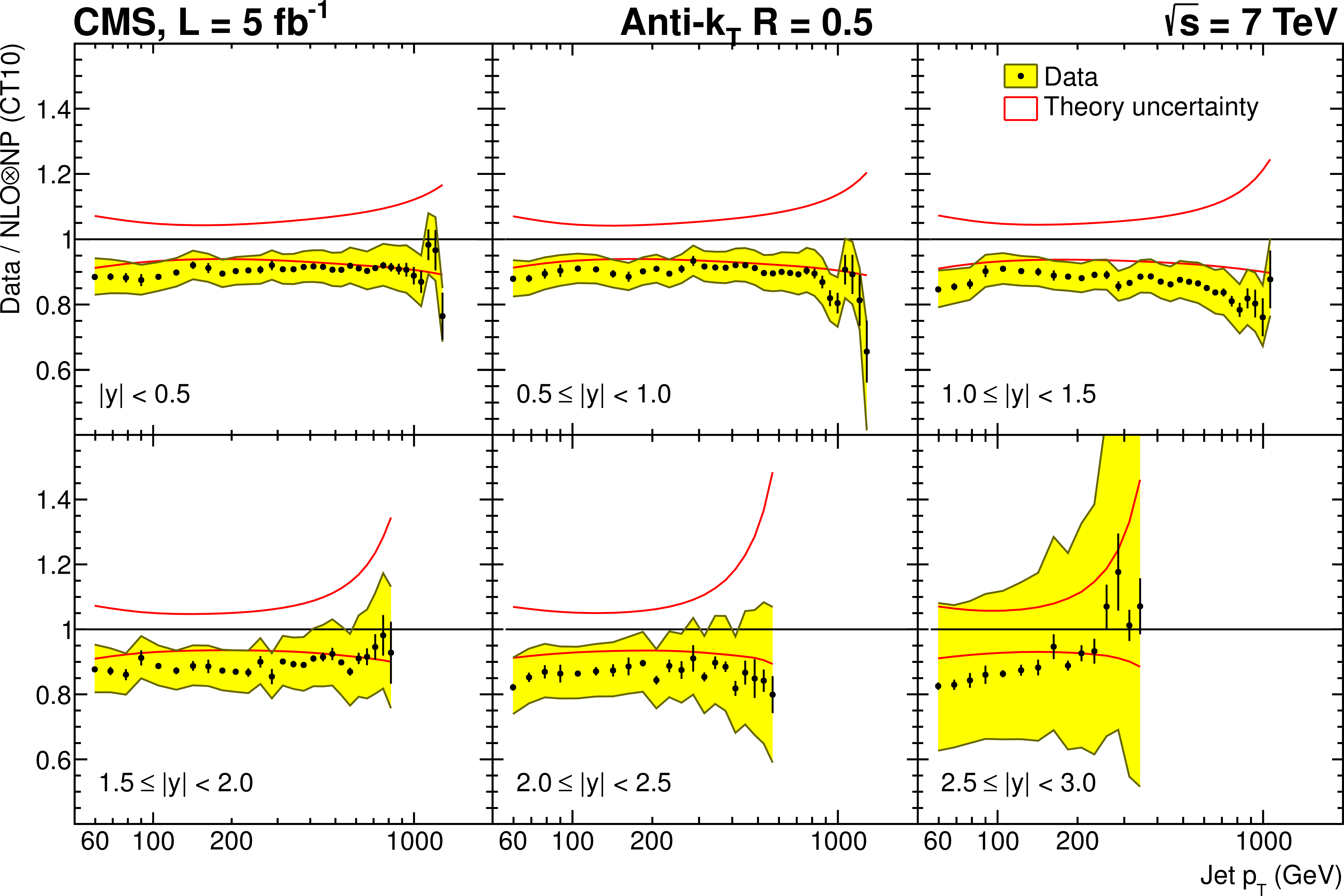
png pdf	Figure 2-a: Inclusive jet cross section with anti-$k_{\mathrm{T}}$ R = 0.5 (a) and R = 0.7 (b) divided by the NLO$\otimes$NP theory prediction using the CT10 NLO PDF set. The statistical and systematic uncertainties are represented by the error bars and the shaded band, respectively. The solid lines indicate the total theory uncertainty. The points with larger error bars occur at trigger boundaries.
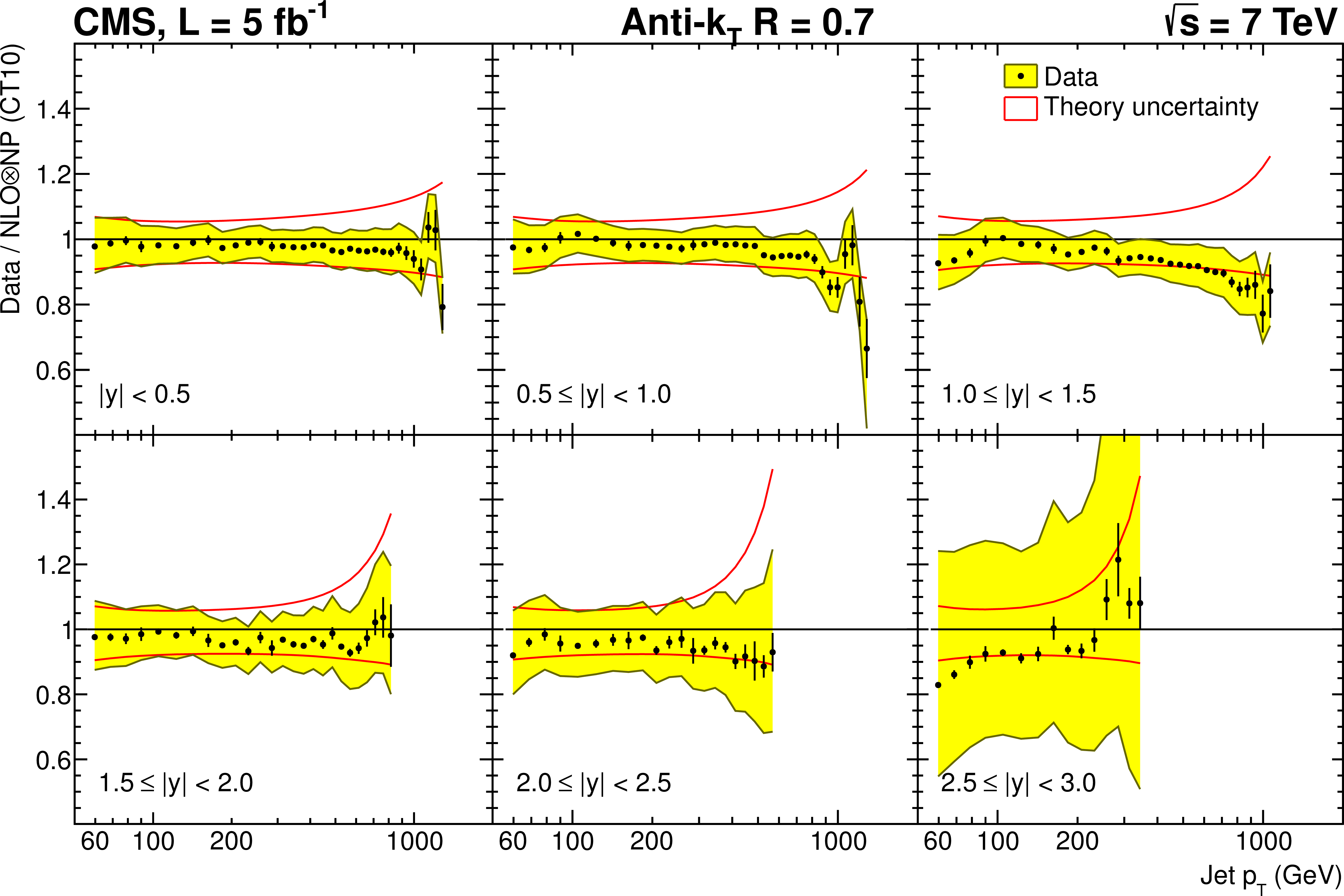
png pdf	Figure 2-b: Inclusive jet cross section with anti-$k_{\mathrm{T}}$ R = 0.5 (a) and R = 0.7 (b) divided by the NLO$\otimes$NP theory prediction using the CT10 NLO PDF set. The statistical and systematic uncertainties are represented by the error bars and the shaded band, respectively. The solid lines indicate the total theory uncertainty. The points with larger error bars occur at trigger boundaries.
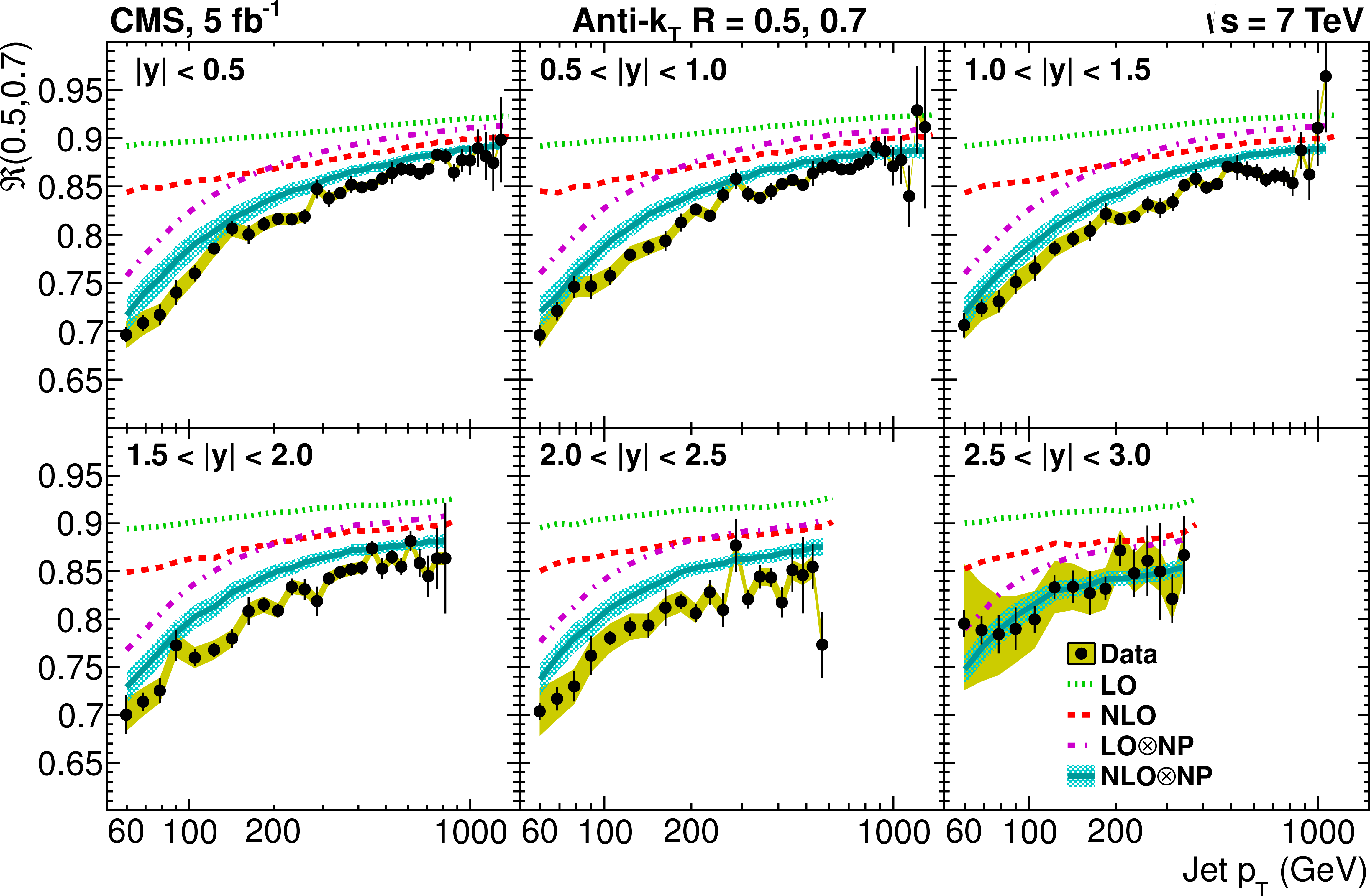
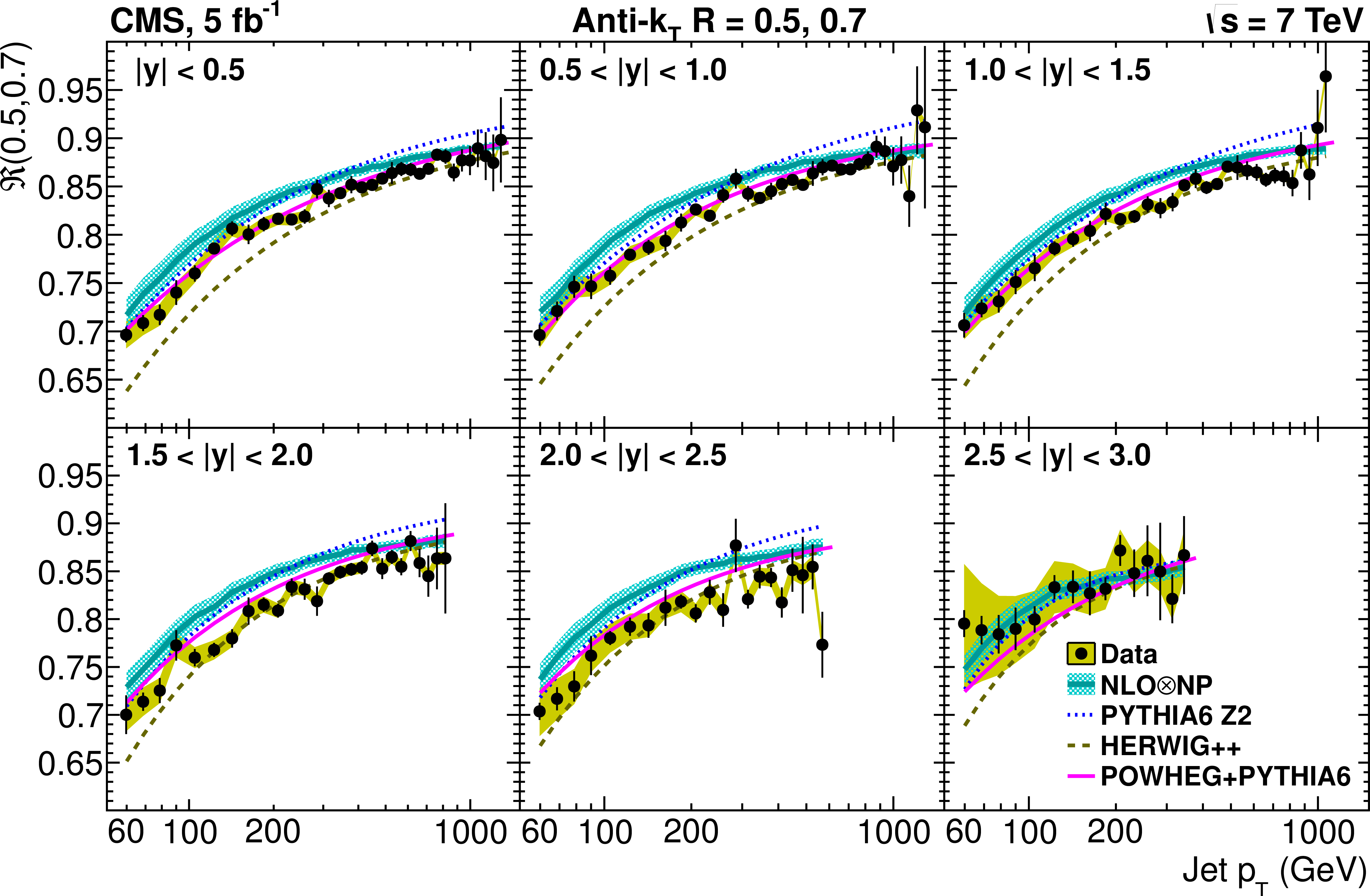
png pdf	Figure 3-a: Jet radius ratio $\mathcal{R}$(0.5, 0.7) in six rapidity bins up to $\|y\| =$ 3.0, compared to LO and NLO with and without NP corrections (a) and versus NLO?NP and MC predictions (b). The error bars on the data points represent the statistical and uncorrelated systematic uncertainty added in quadrature, and the shaded bands represent correlated systematic uncertainty. The NLO calculation was provided by G. Soyez [26].
png pdf	Figure 3-b: Jet radius ratio $\mathcal{R}$(0.5, 0.7) in six rapidity bins up to $\|y\| =$ 3.0, compared to LO and NLO with and without NP corrections (a) and versus NLO?NP and MC predictions (b). The error bars on the data points represent the statistical and uncorrelated systematic uncertainty added in quadrature, and the shaded bands represent correlated systematic uncertainty. The NLO calculation was provided by G. Soyez [26].
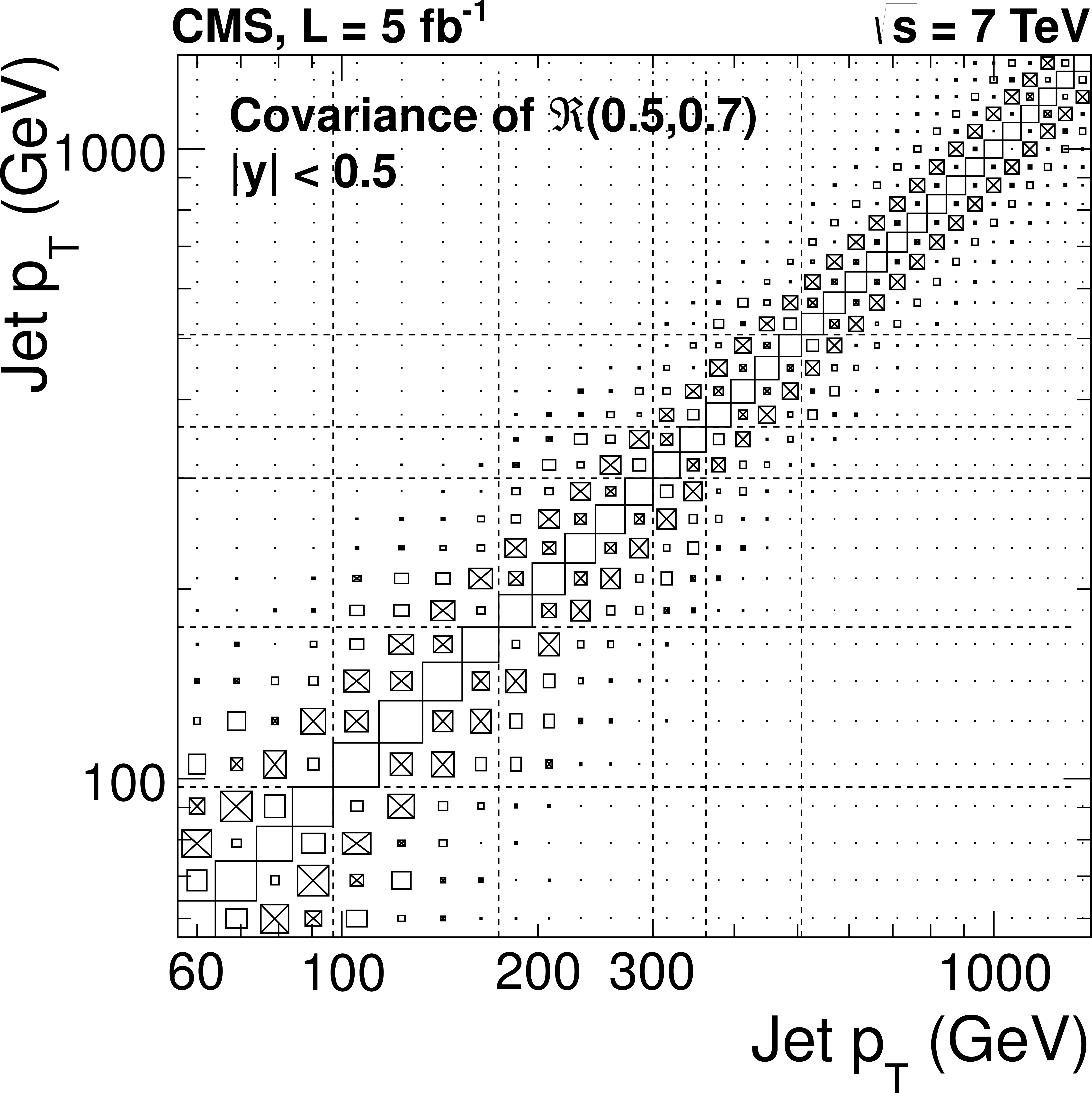
png pdf	Figure 4-a: (a) Covariance matrix $\mathcal{U}$ for the jet radius ratio $\mathcal{R}$(0.5,0.7), normalized by the diagonal elements to show the level of correlation. Dashed horizontal and vertical lines indicate the analysis $p_{\mathrm{T}}$ thresholds corresponding to different triggers. The size of the boxes relative to bin size is proportional to the correlation coefficient in the range from -1 to 1. The diagonal elements are 1 and thus indicative of the variable bin size. The crossed boxes corresponds to anticorrelation, while the open boxes correspond to positive correlations between two bins. (b) Comparison of the square root of the covariance matrix diagonals with a random sampling estimate using the delete-$d$ (d = 10%) jackknife method. The differences between the full data set and the ten delete-$d$ samples are shown by the full circles.
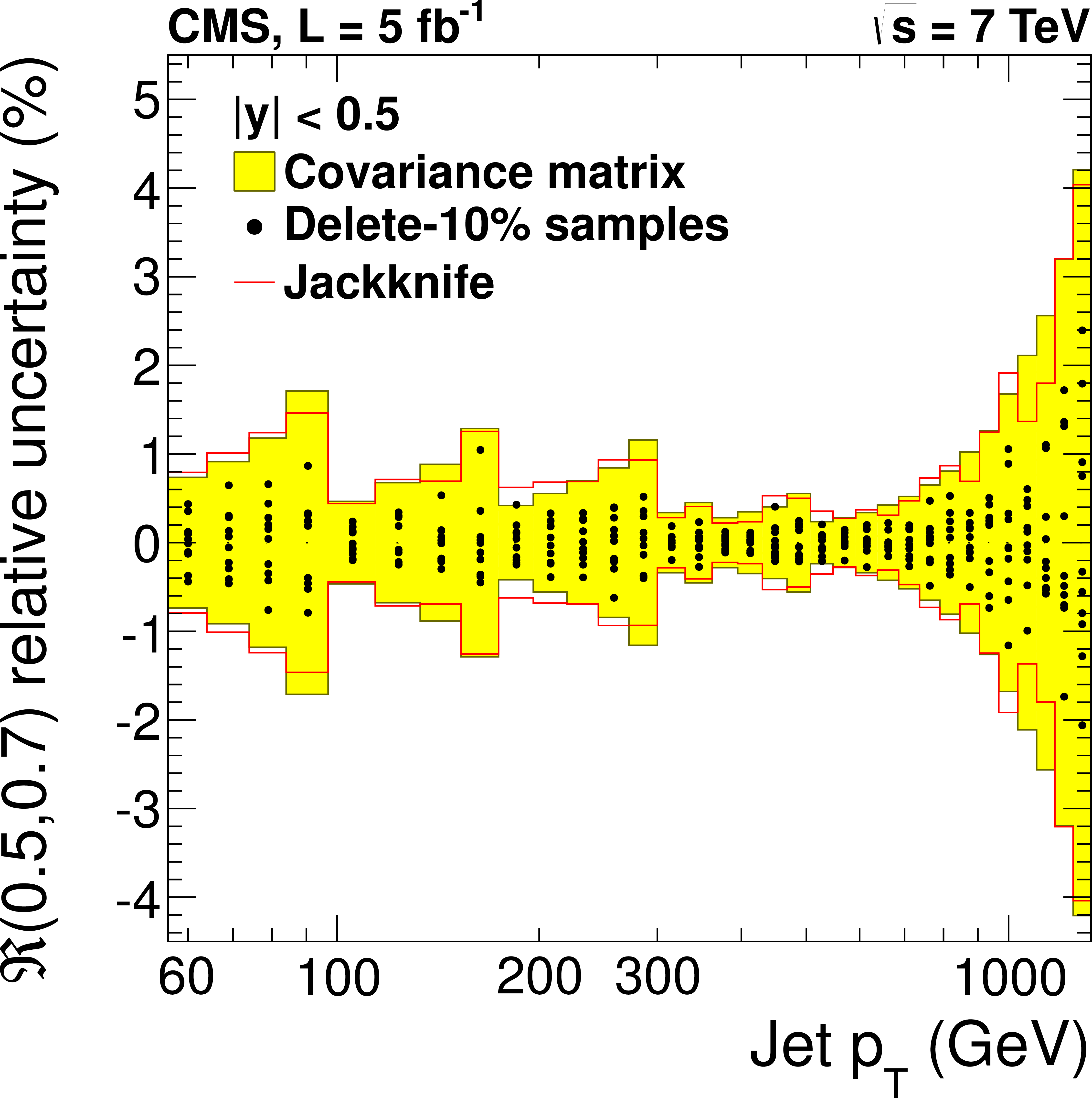
png pdf	Figure 4-b: (a) Covariance matrix $\mathcal{U}$ for the jet radius ratio $\mathcal{R}$(0.5,0.7), normalized by the diagonal elements to show the level of correlation. Dashed horizontal and vertical lines indicate the analysis $p_{\mathrm{T}}$ thresholds corresponding to different triggers. The size of the boxes relative to bin size is proportional to the correlation coefficient in the range from -1 to 1. The diagonal elements are 1 and thus indicative of the variable bin size. The crossed boxes corresponds to anticorrelation, while the open boxes correspond to positive correlations between two bins. (b) Comparison of the square root of the covariance matrix diagonals with a random sampling estimate using the delete-$d$ (d = 10%) jackknife method. The differences between the full data set and the ten delete-$d$ samples are shown by the full circles.