

Compact Muon Solenoid
LHC, CERN
| CMS-SMP-14-005 ; CERN-PH-EP-2015-089 | ||
| Comparison of the Z$/\gamma^{*}$+jets to $\gamma$+jets cross sections in pp collisions at $\sqrt{s} =$ 8 TeV | ||
| CMS Collaboration | ||
| 25 May 2015 | ||
| J. High Energy Phys. 10 (2015) 128 [Erratum] | ||
|
Abstract:
A comparison of the differential cross sections for the processes Z$/\gamma^{*}$+jets and photon ($\gamma$)+jets is presented. The measurements are based on data collected with the CMS detector at $\sqrt{s} =$ 8 TeV corresponding to an integrated luminosity of 19.7 fb$^{-1}$. The differential cross sections and their ratios are presented as functions of $ p_{ \mathrm{T} } $. The measurements are also shown as functions of the jet multiplicity. Differential cross sections are obtained as functions of the ratio of the Z$/\gamma^{*}$ $ p_{ \mathrm{T} } $ to the sum of all jet transverse momenta and of the ratio of the Z$/\gamma^{*}$ $ p_{ \mathrm{T} } $ to the leading jet transverse momentum. The data are corrected for detector effects and are compared to simulations based on several QCD calculations. Erratum: An error was found in the published version in the (b) plots in Fig. 2 and Fig. 3. In both cases the normalization of the photon plots is incorrect by the factor of the luminosity of 19.7. The figures shown in this page are the corrected ones. The physics conclusion of the paper remains unchanged, since the ratio plots are unaffected [J. High Energy Phys. 04 (2016) 010]. | ||
| Links: e-print arXiv:1505.06520 [hep-ex] (PDF) ; CDS record ; inSPIRE record ; Public twiki page ; HepData record ; CADI line (restricted) ; | ||
| Figures & Tables | Summary | Additional Figures | CMS Publications |
|---|
| Figures | |
png pdf |
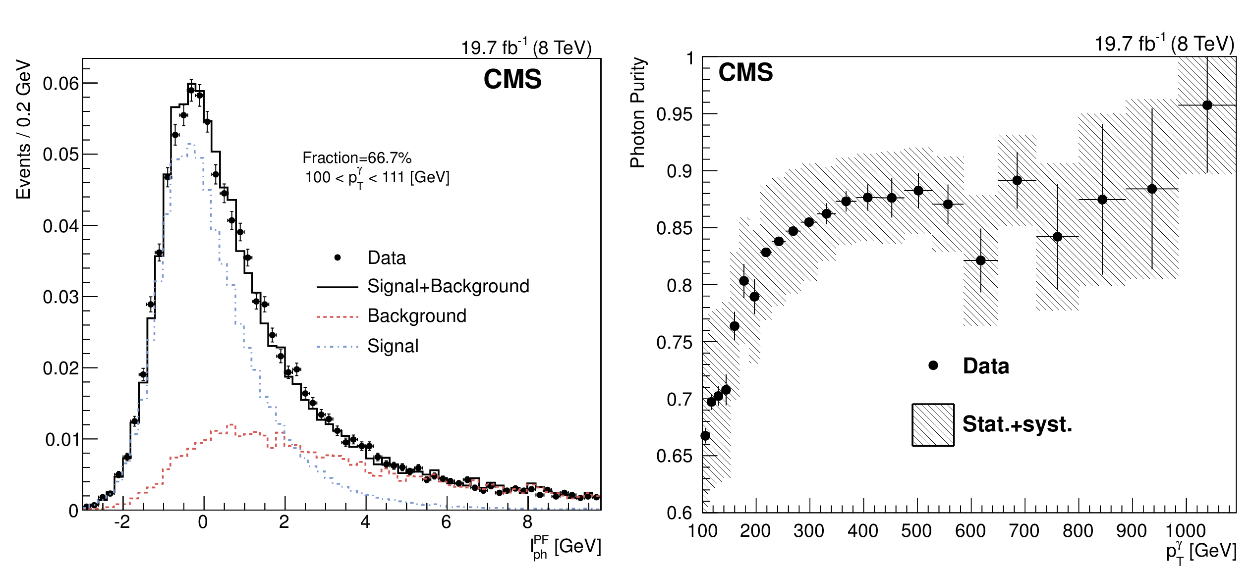
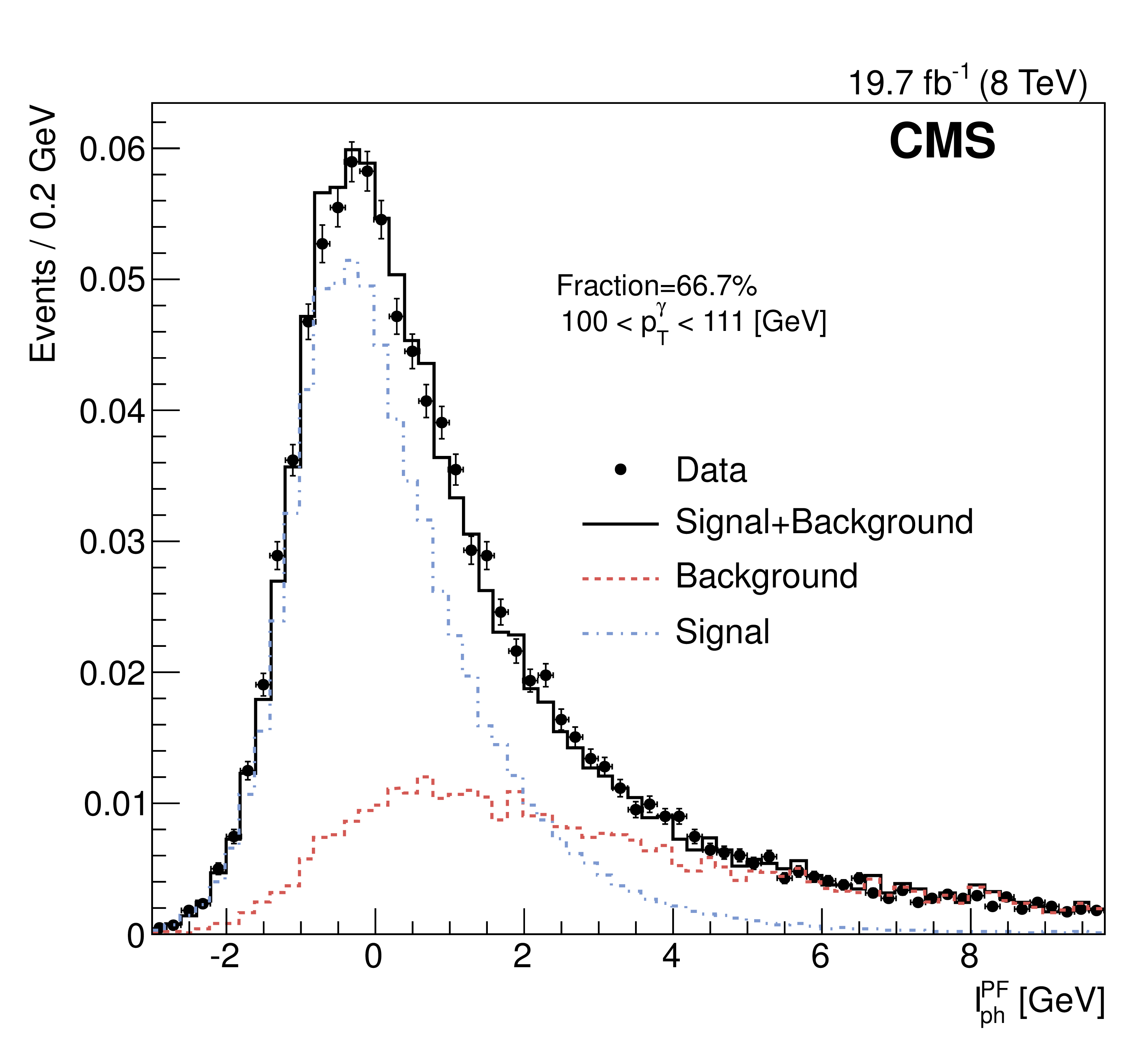
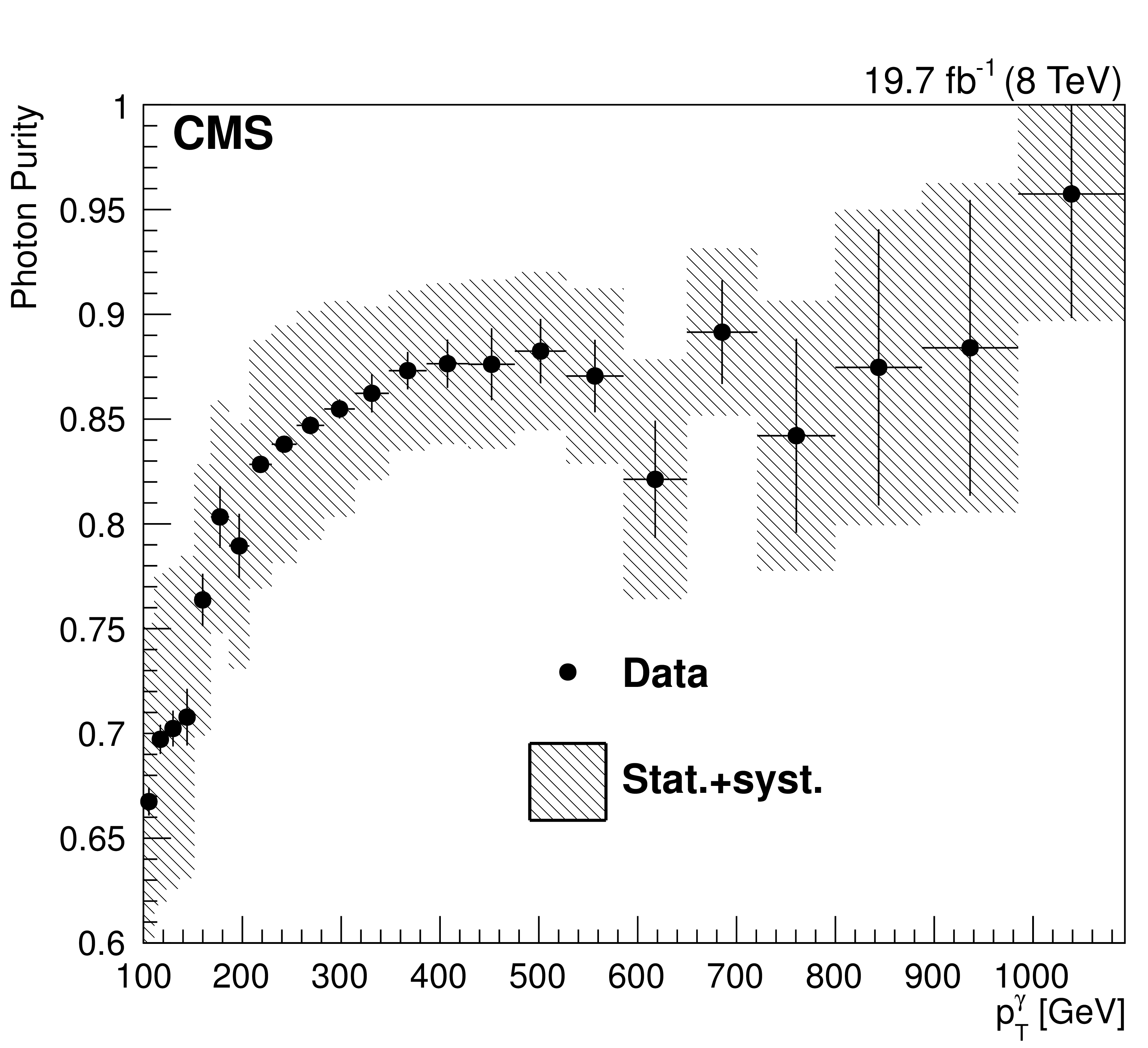
Figure 1:
The purity fit on the photon component of the photon isolation $I_\text {ph}^\mathrm {PF}$ in the photon transverse momentum bin between 100 and 111 GeV in data (a). The photon purity as function of the photon transverse momentum (b). The dots are the data points, the dot-dashed line is the signal template, and the dotted line represents the background component. The solid line represents the fit and the legend shows the resulting purity fraction of 66.7%. |
png pdf |
Figure 1-a:
The purity fit on the photon component of the photon isolation $I_\text {ph}^\mathrm {PF}$ in the photon transverse momentum bin between 100 and 111 GeV in data (a). The photon purity as function of the photon transverse momentum (b). The dots are the data points, the dot-dashed line is the signal template, and the dotted line represents the background component. The solid line represents the fit and the legend shows the resulting purity fraction of 66.7%. |
png pdf |
Figure 1-b:
The purity fit on the photon component of the photon isolation $I_\text {ph}^\mathrm {PF}$ in the photon transverse momentum bin between 100 and 111 GeV in data (a). The photon purity as function of the photon transverse momentum (b). The dots are the data points, the dot-dashed line is the signal template, and the dotted line represents the background component. The solid line represents the fit and the legend shows the resulting purity fraction of 66.7%. |
png pdf |
Figure 1-c:
The purity fit on the photon component of the photon isolation $I_\text {ph}^\mathrm {PF}$ in the photon transverse momentum bin between 100 and 111 GeV in data (a). The photon purity as function of the photon transverse momentum (b). The dots are the data points, the dot-dashed line is the signal template, and the dotted line represents the background component. The solid line represents the fit and the legend shows the resulting purity fraction of 66.7%. |

png pdf |
Figure 1-d:
The purity fit on the photon component of the photon isolation $I_\text {ph}^\mathrm {PF}$ in the photon transverse momentum bin between 100 and 111 GeV in data (a). The photon purity as function of the photon transverse momentum (b). The dots are the data points, the dot-dashed line is the signal template, and the dotted line represents the background component. The solid line represents the fit and the legend shows the resulting purity fraction of 66.7%. |
png pdf |
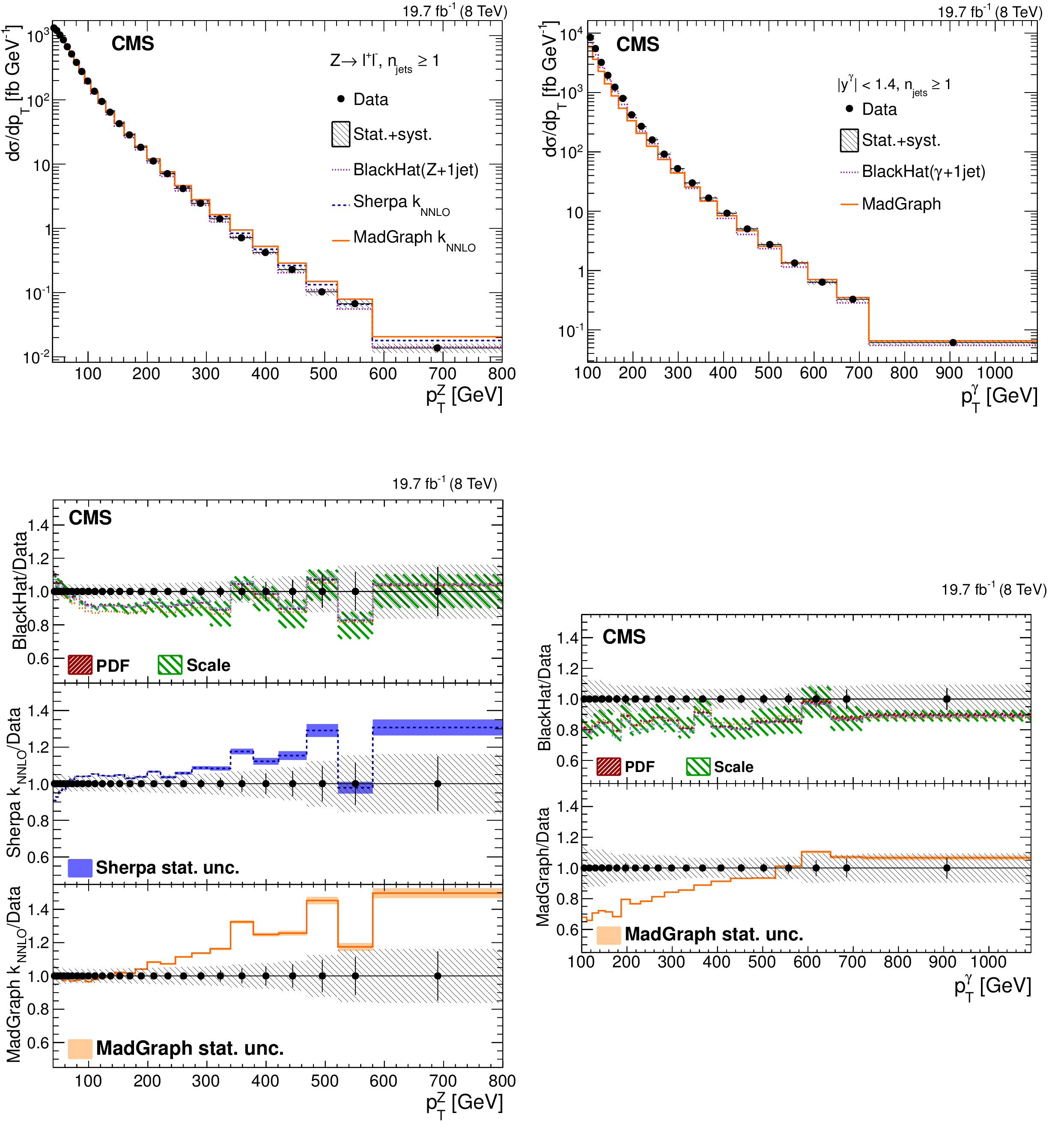
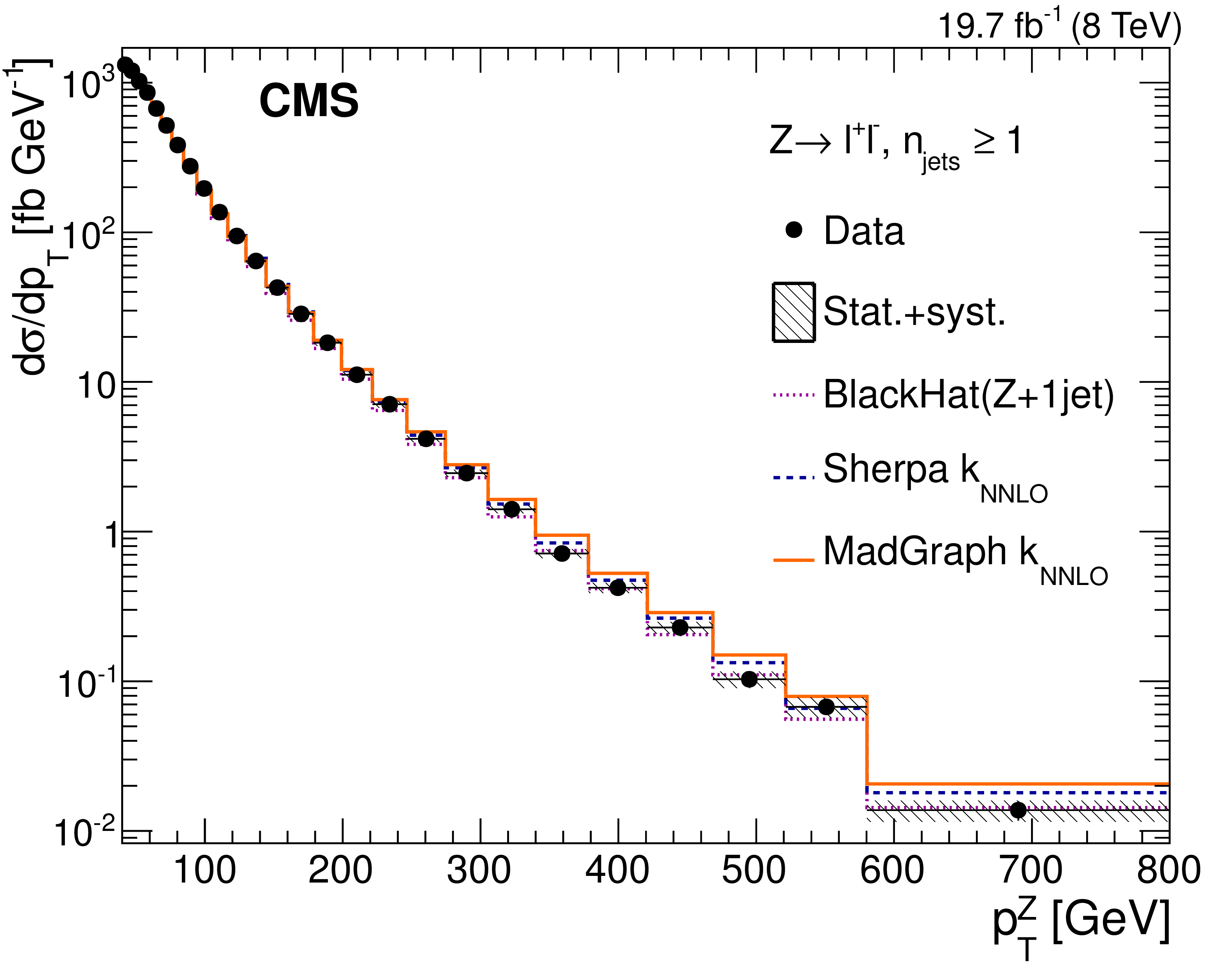
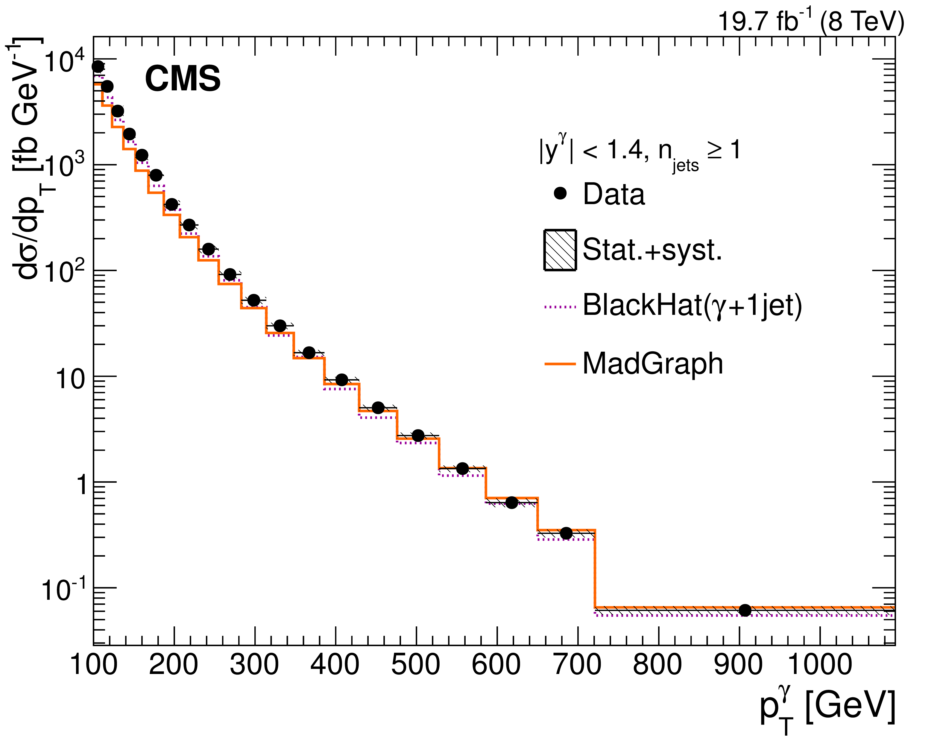
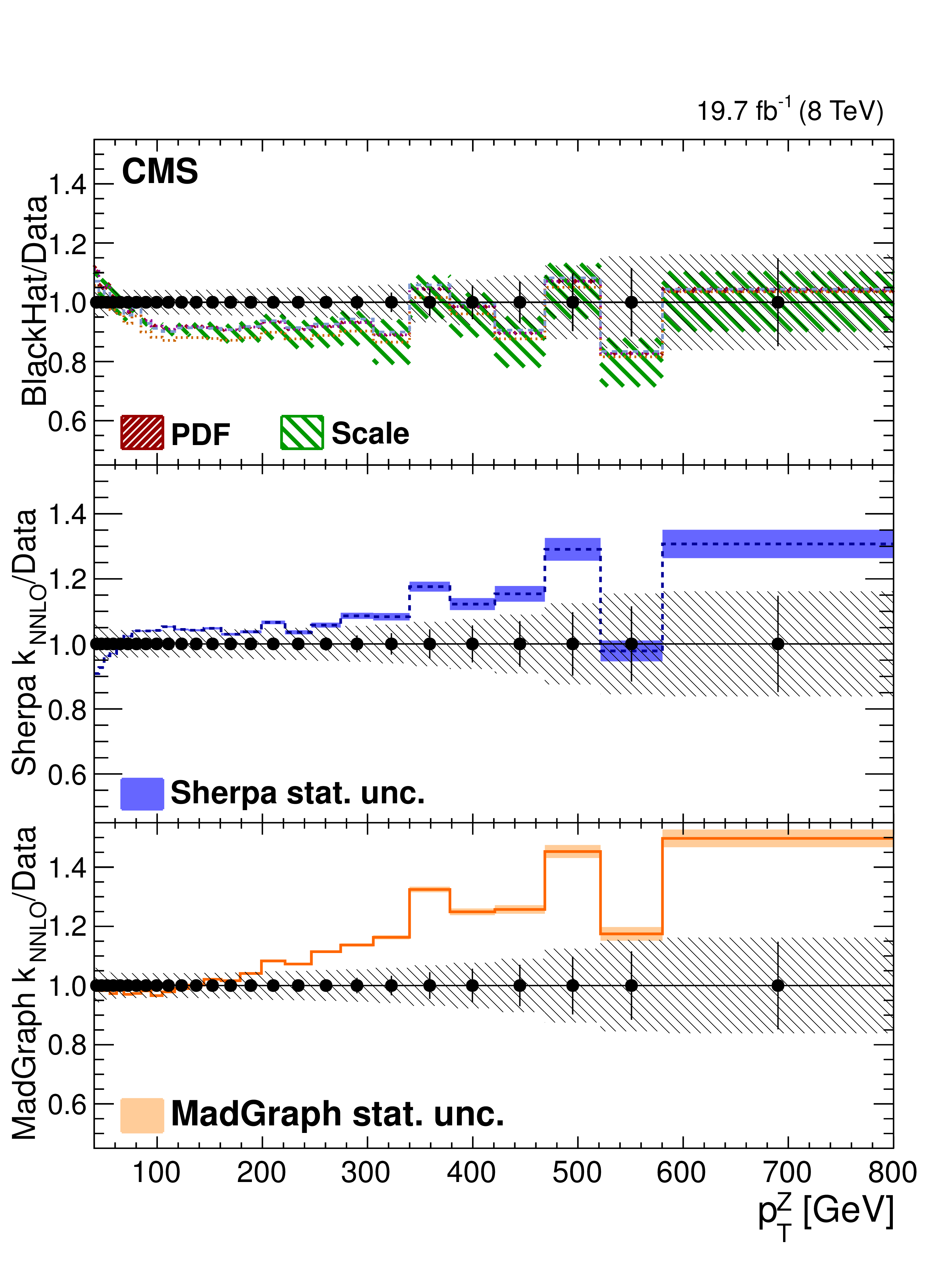
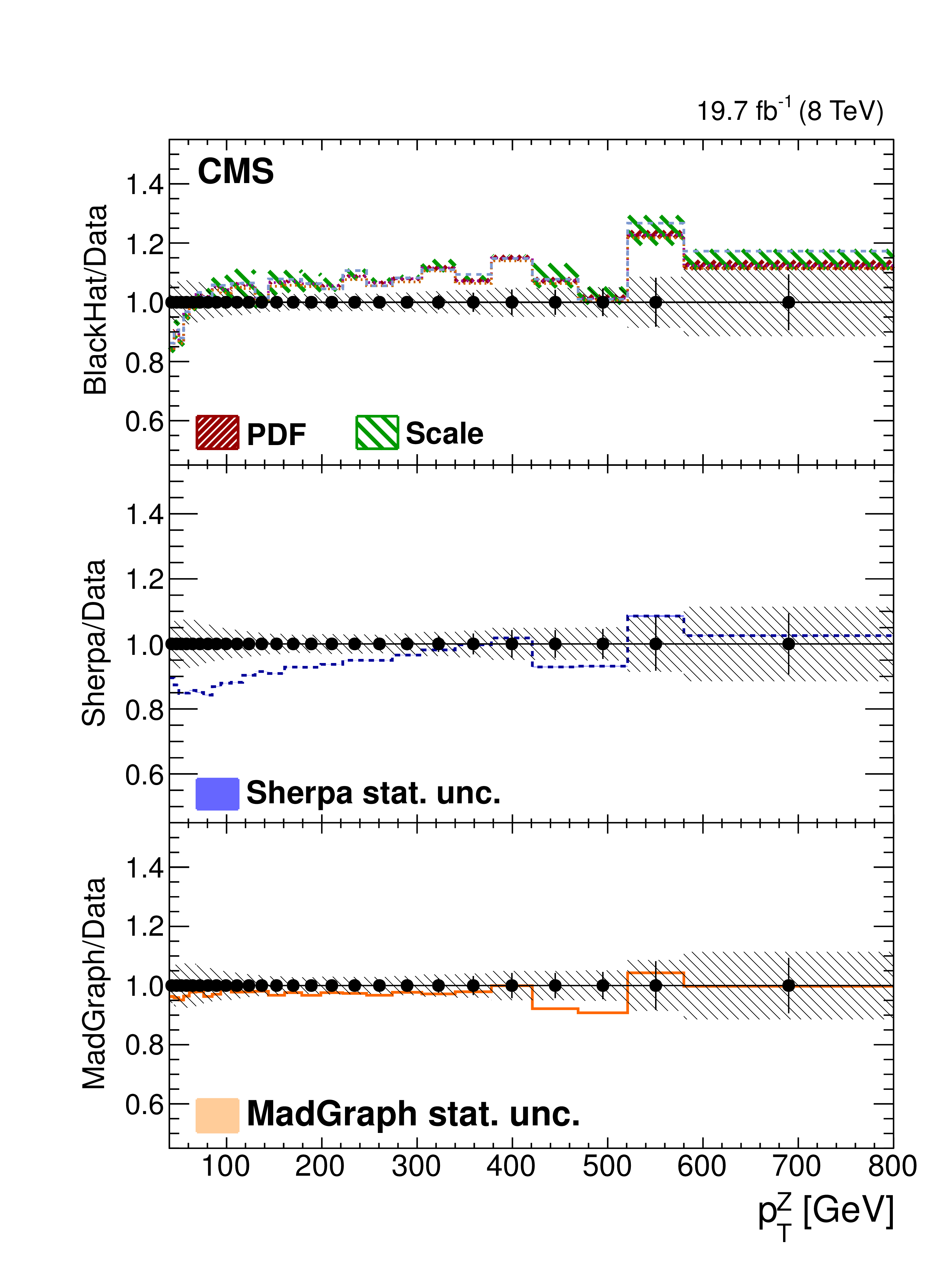
Figure 2:
a: Differential cross section for Z boson production as a function of $ { {p_{\mathrm {T}}} ^{ {\mathrm {Z}}}} $ for an inclusive Z+jets, $ {n_{\text {jets}}} \geq 1$ selection of detector-corrected data in comparison with estimations from MadGraph+Pythia6, Sherpa, and Blackhat. b: Differential cross section for photon production as a function of $ {p_{\mathrm {T}}} ^{\gamma }$ for an inclusive $\gamma$+jets, $ {n_{\text {jets}}} \geq 1$ selection for central rapidities $ {| y^{\gamma } | }<1.4$ in detector-corrected data is compared with estimations from MadGraph+Pythia6 and Blackhat. A detailed explanation is given in the Section on Differential Cross-Sections. The bottom plots give the ratio of the various theoretical estimations to the data in the Z+jets case (c) and $\gamma$+jets case (d). |
png pdf |
Figure 2-a:
a: Differential cross section for Z boson production as a function of $ { {p_{\mathrm {T}}} ^{ {\mathrm {Z}}}} $ for an inclusive Z+jets, $ {n_{\text {jets}}} \geq 1$ selection of detector-corrected data in comparison with estimations from MadGraph+Pythia6, Sherpa, and Blackhat. b: Differential cross section for photon production as a function of $ {p_{\mathrm {T}}} ^{\gamma }$ for an inclusive $\gamma$+jets, $ {n_{\text {jets}}} \geq 1$ selection for central rapidities $ {| y^{\gamma } | }<1.4$ in detector-corrected data is compared with estimations from MadGraph+Pythia6 and Blackhat. A detailed explanation is given in the Section on Differential Cross-Sections. The bottom plots give the ratio of the various theoretical estimations to the data in the Z+jets case (c) and $\gamma$+jets case (d). |
png pdf |
Figure 2-b:
a: Differential cross section for Z boson production as a function of $ { {p_{\mathrm {T}}} ^{ {\mathrm {Z}}}} $ for an inclusive Z+jets, $ {n_{\text {jets}}} \geq 1$ selection of detector-corrected data in comparison with estimations from MadGraph+Pythia6, Sherpa, and Blackhat. b: Differential cross section for photon production as a function of $ {p_{\mathrm {T}}} ^{\gamma }$ for an inclusive $\gamma$+jets, $ {n_{\text {jets}}} \geq 1$ selection for central rapidities $ {| y^{\gamma } | }<1.4$ in detector-corrected data is compared with estimations from MadGraph+Pythia6 and Blackhat. A detailed explanation is given in the Section on Differential Cross-Sections. The bottom plots give the ratio of the various theoretical estimations to the data in the Z+jets case (c) and $\gamma$+jets case (d). |
png pdf |
Figure 2-c:
a: Differential cross section for Z boson production as a function of $ { {p_{\mathrm {T}}} ^{ {\mathrm {Z}}}} $ for an inclusive Z+jets, $ {n_{\text {jets}}} \geq 1$ selection of detector-corrected data in comparison with estimations from MadGraph+Pythia6, Sherpa, and Blackhat. b: Differential cross section for photon production as a function of $ {p_{\mathrm {T}}} ^{\gamma }$ for an inclusive $\gamma$+jets, $ {n_{\text {jets}}} \geq 1$ selection for central rapidities $ {| y^{\gamma } | }<1.4$ in detector-corrected data is compared with estimations from MadGraph+Pythia6 and Blackhat. A detailed explanation is given in the Section on Differential Cross-Sections. The bottom plots give the ratio of the various theoretical estimations to the data in the Z+jets case (c) and $\gamma$+jets case (d). |

png pdf |
Figure 2-d:
a: Differential cross section for Z boson production as a function of $ { {p_{\mathrm {T}}} ^{ {\mathrm {Z}}}} $ for an inclusive Z+jets, $ {n_{\text {jets}}} \geq 1$ selection of detector-corrected data in comparison with estimations from MadGraph+Pythia6, Sherpa, and Blackhat. b: Differential cross section for photon production as a function of $ {p_{\mathrm {T}}} ^{\gamma }$ for an inclusive $\gamma$+jets, $ {n_{\text {jets}}} \geq 1$ selection for central rapidities $ {| y^{\gamma } | }<1.4$ in detector-corrected data is compared with estimations from MadGraph+Pythia6 and Blackhat. A detailed explanation is given in the Section on Differential Cross-Sections. The bottom plots give the ratio of the various theoretical estimations to the data in the Z+jets case (c) and $\gamma$+jets case (d). |

png pdf |
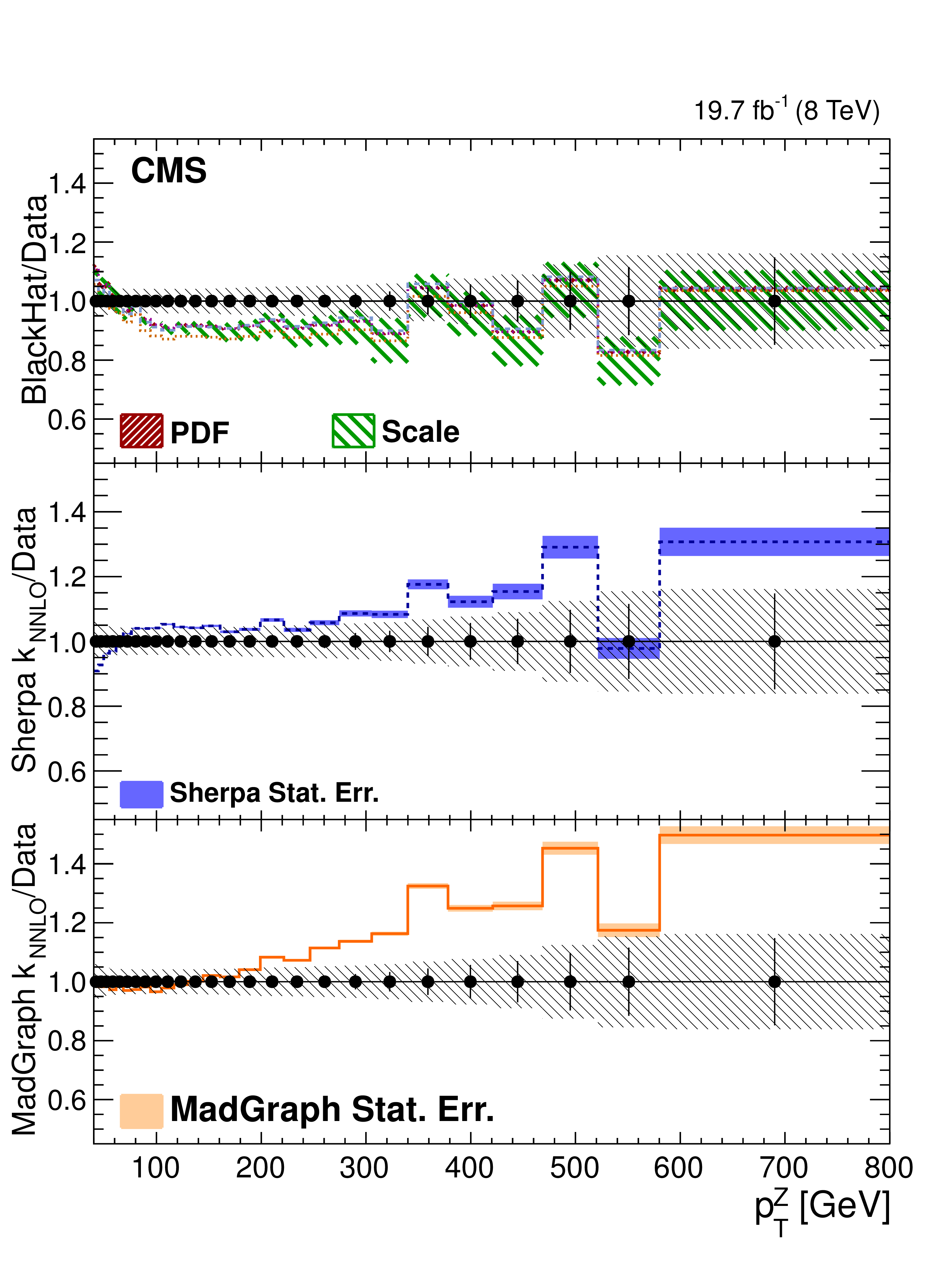
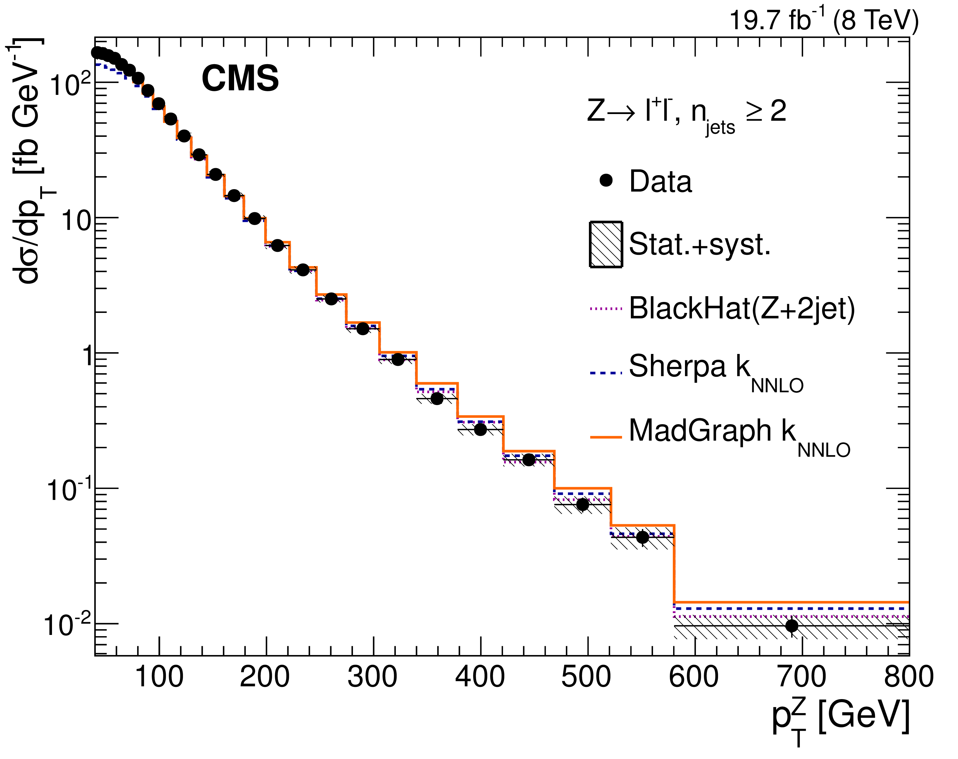
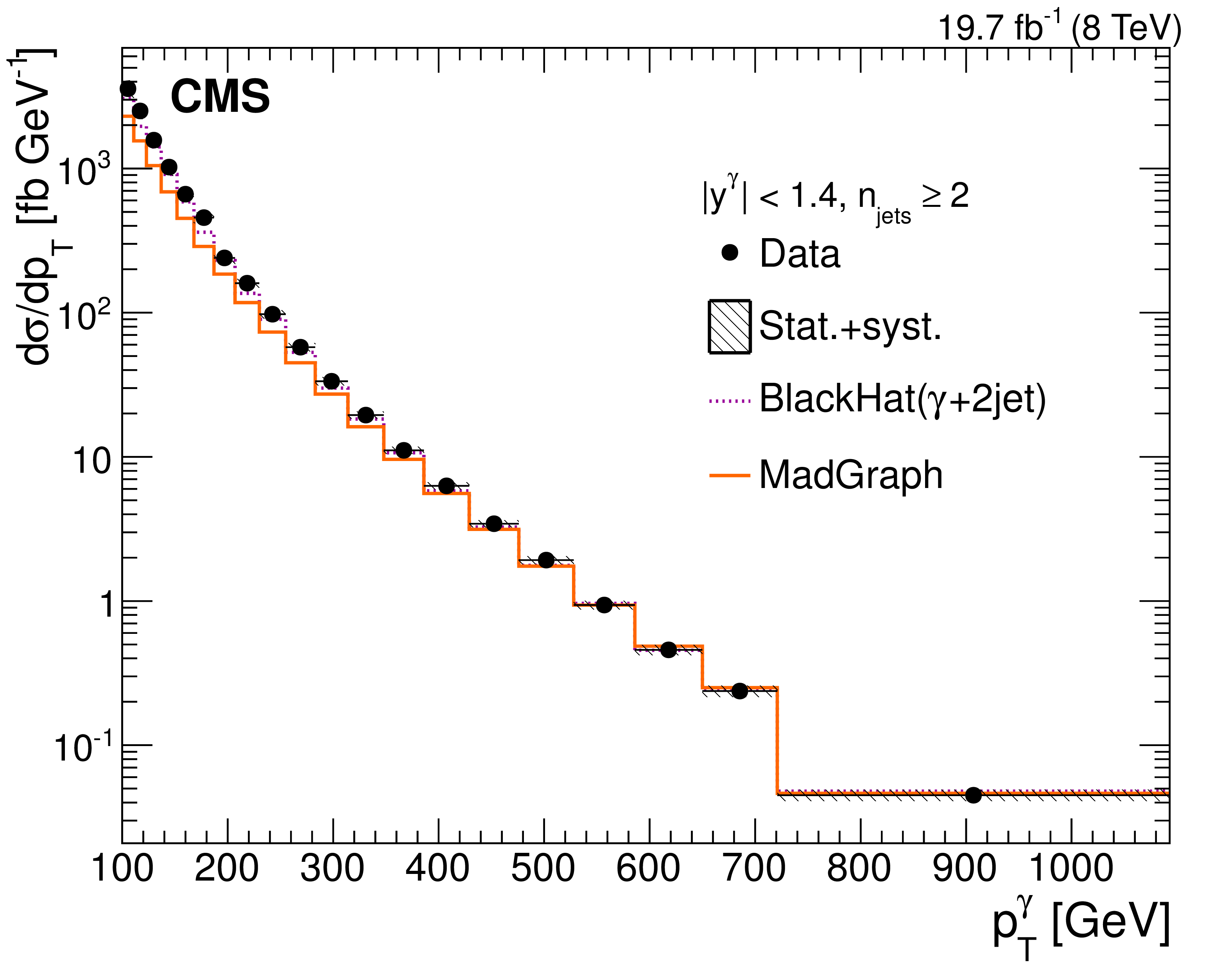
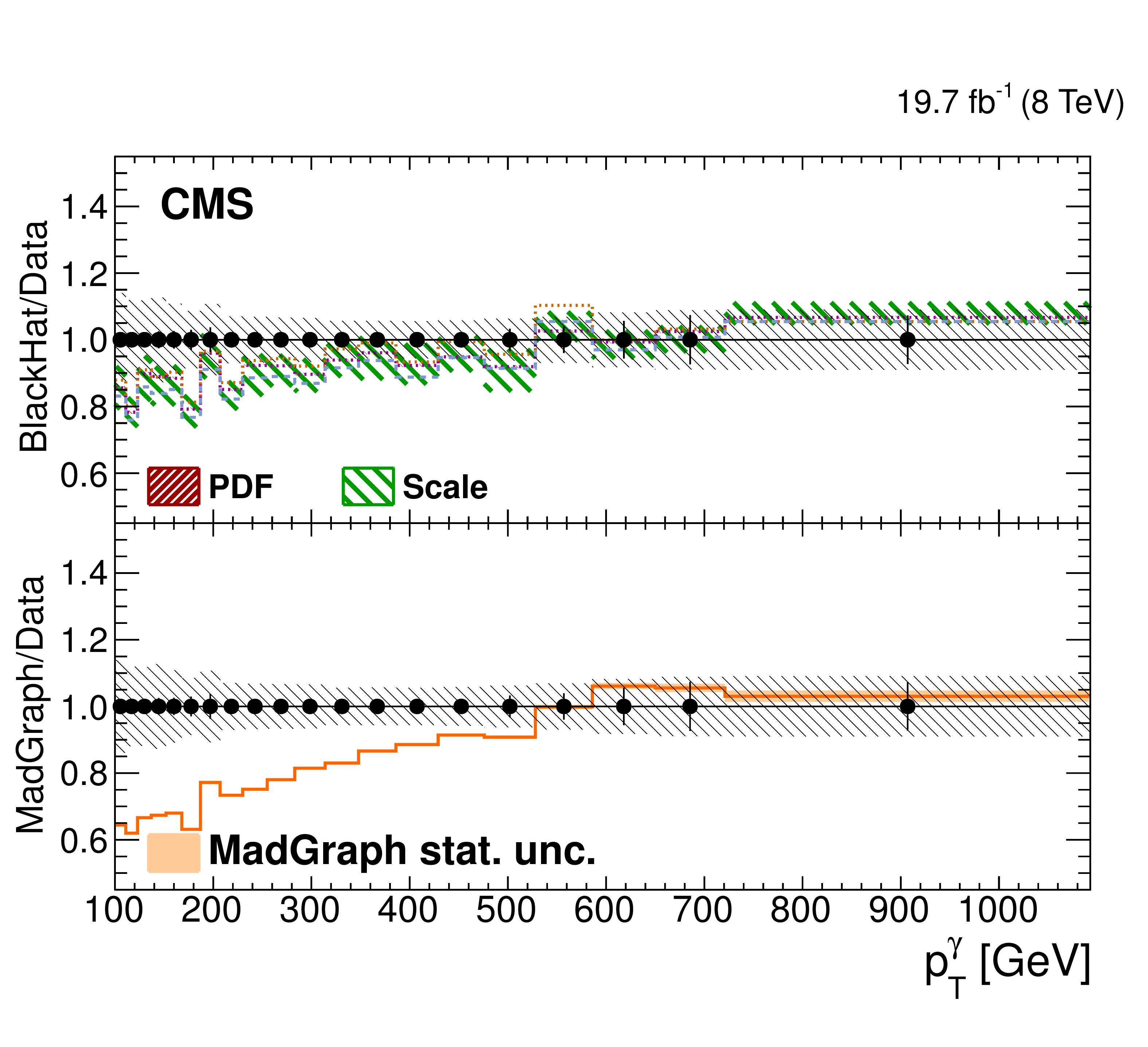
Figure 3:
a: Differential cross section for Z boson production as a function of $ { {p_{\mathrm {T}}} ^{ {\mathrm {Z}}}} $ for an inclusive Z+jets, $ {n_{\text {jets}}} \geq 2$ selection of detector-corrected data in comparison with estimations from MadGraph+Pythia6, Sherpa, and Blackhat. b: Differential cross section for photon production as a function of $ {p_{\mathrm {T}}} ^{\gamma }$ for an inclusive $ \gamma $+jets, $ {n_{\text {jets}}} \geq 2$ selection for central rapidities $ {| y^{\gamma } | }<1.4$ in detector-corrected data is compared with estimations from MadGraph+Pythia6and . A detailed explanation is given in the Section on Differential Cross-Sections. The bottom plots give the ratio of the various theoretical estimations to the data in the Z+jets case (c) and $\gamma$+jets case (d). |
png pdf |
Figure 3-a:
a: Differential cross section for Z boson production as a function of $ { {p_{\mathrm {T}}} ^{ {\mathrm {Z}}}} $ for an inclusive Z+jets, $ {n_{\text {jets}}} \geq 2$ selection of detector-corrected data in comparison with estimations from MadGraph+Pythia6, Sherpa, and Blackhat. b: Differential cross section for photon production as a function of $ {p_{\mathrm {T}}} ^{\gamma }$ for an inclusive $ \gamma $+jets, $ {n_{\text {jets}}} \geq 2$ selection for central rapidities $ {| y^{\gamma } | }<1.4$ in detector-corrected data is compared with estimations from MadGraph+Pythia6and . A detailed explanation is given in the Section on Differential Cross-Sections. The bottom plots give the ratio of the various theoretical estimations to the data in the Z+jets case (c) and $\gamma$+jets case (d). |
png pdf |
Figure 3-b:
a: Differential cross section for Z boson production as a function of $ { {p_{\mathrm {T}}} ^{ {\mathrm {Z}}}} $ for an inclusive Z+jets, $ {n_{\text {jets}}} \geq 2$ selection of detector-corrected data in comparison with estimations from MadGraph+Pythia6, Sherpa, and Blackhat. b: Differential cross section for photon production as a function of $ {p_{\mathrm {T}}} ^{\gamma }$ for an inclusive $ \gamma $+jets, $ {n_{\text {jets}}} \geq 2$ selection for central rapidities $ {| y^{\gamma } | }<1.4$ in detector-corrected data is compared with estimations from MadGraph+Pythia6and . A detailed explanation is given in the Section on Differential Cross-Sections. The bottom plots give the ratio of the various theoretical estimations to the data in the Z+jets case (c) and $\gamma$+jets case (d). |

png pdf |
Figure 3-c:
a: Differential cross section for Z boson production as a function of $ { {p_{\mathrm {T}}} ^{ {\mathrm {Z}}}} $ for an inclusive Z+jets, $ {n_{\text {jets}}} \geq 2$ selection of detector-corrected data in comparison with estimations from MadGraph+Pythia6, Sherpa, and Blackhat. b: Differential cross section for photon production as a function of $ {p_{\mathrm {T}}} ^{\gamma }$ for an inclusive $ \gamma $+jets, $ {n_{\text {jets}}} \geq 2$ selection for central rapidities $ {| y^{\gamma } | }<1.4$ in detector-corrected data is compared with estimations from MadGraph+Pythia6and . A detailed explanation is given in the Section on Differential Cross-Sections. The bottom plots give the ratio of the various theoretical estimations to the data in the Z+jets case (c) and $\gamma$+jets case (d). |
png pdf |
Figure 3-d:
a: Differential cross section for Z boson production as a function of $ { {p_{\mathrm {T}}} ^{ {\mathrm {Z}}}} $ for an inclusive Z+jets, $ {n_{\text {jets}}} \geq 2$ selection of detector-corrected data in comparison with estimations from MadGraph+Pythia6, Sherpa, and Blackhat. b: Differential cross section for photon production as a function of $ {p_{\mathrm {T}}} ^{\gamma }$ for an inclusive $ \gamma $+jets, $ {n_{\text {jets}}} \geq 2$ selection for central rapidities $ {| y^{\gamma } | }<1.4$ in detector-corrected data is compared with estimations from MadGraph+Pythia6and . A detailed explanation is given in the Section on Differential Cross-Sections. The bottom plots give the ratio of the various theoretical estimations to the data in the Z+jets case (c) and $\gamma$+jets case (d). |
png pdf |
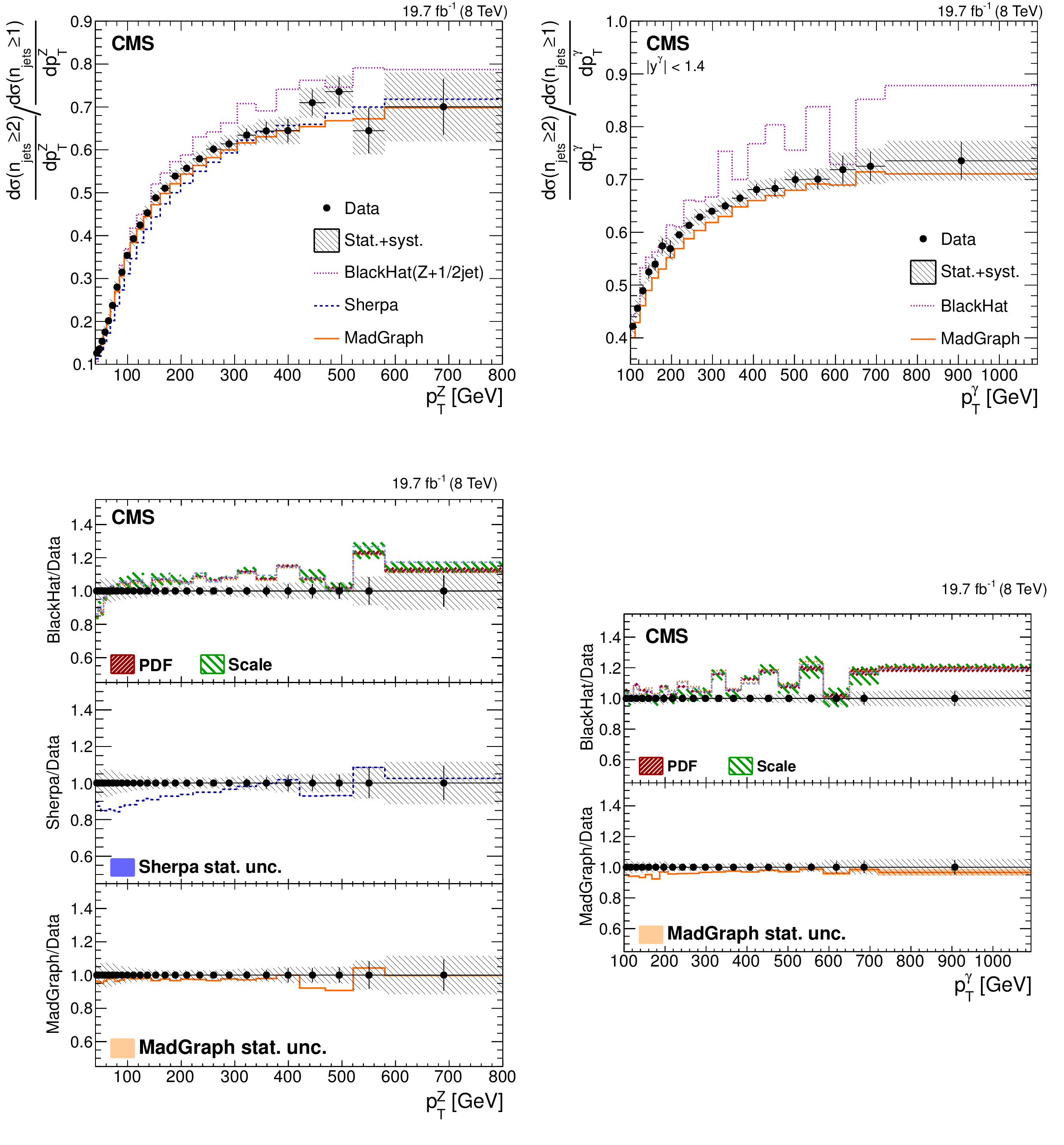
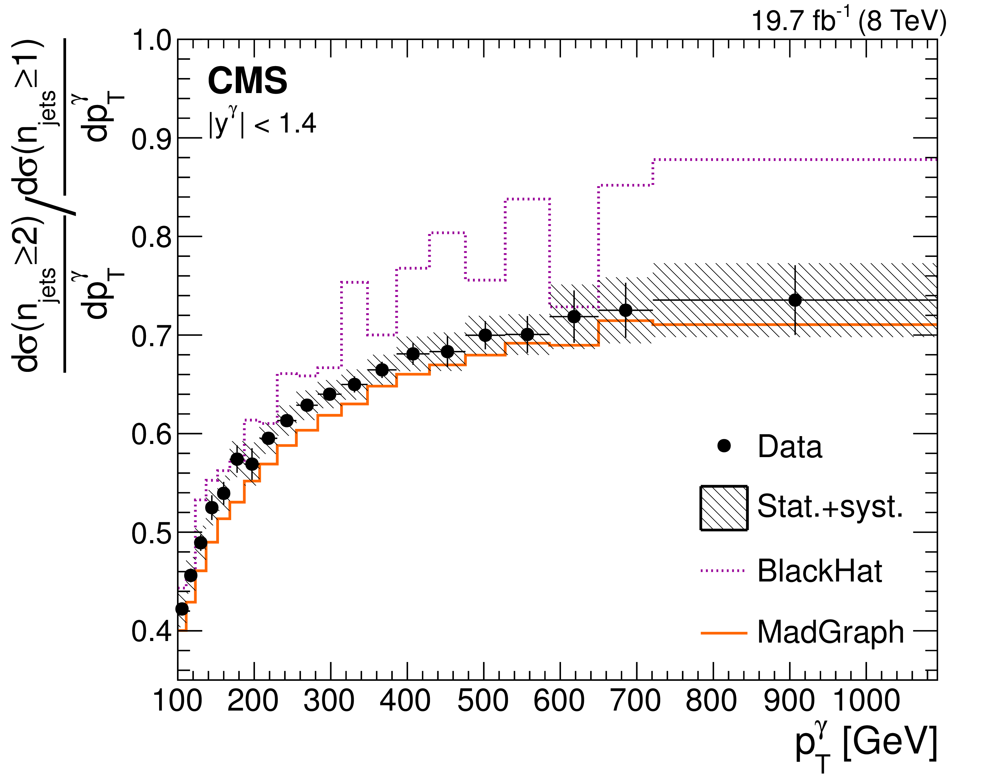
Figure 4:
Ratio of the inclusive rates for $ {n_{\text {jets}}} \geq 2$ and $ {n_{\text {jets}}} \geq 1$ versus the transverse momentum of the boson for Z+jets in detector-corrected data compared to estimations from MadGraph+Pythia6, Sherpa, and Blackhat (a) and for $ \gamma $+jets for central rapidities $ {| y^{\gamma } | }<1.4$ in detector-corrected data compared with estimations from MadGraph+Pythia6 and Blackhat (b). A detailed explanation is given in the Section on Differential Cross-Sections. The bottom plots give the ratio of the various theoretical estimations to the data in the Z+jets case (c) and $\gamma$+jets case (d). |

png pdf |
Figure 4-a:
Ratio of the inclusive rates for $ {n_{\text {jets}}} \geq 2$ and $ {n_{\text {jets}}} \geq 1$ versus the transverse momentum of the boson for Z+jets in detector-corrected data compared to estimations from MadGraph+Pythia6, Sherpa, and Blackhat (a) and for $ \gamma $+jets for central rapidities $ {| y^{\gamma } | }<1.4$ in detector-corrected data compared with estimations from MadGraph+Pythia6 and Blackhat (b). A detailed explanation is given in the Section on Differential Cross-Sections. The bottom plots give the ratio of the various theoretical estimations to the data in the Z+jets case (c) and $\gamma$+jets case (d). |
png pdf |
Figure 4-b:
Ratio of the inclusive rates for $ {n_{\text {jets}}} \geq 2$ and $ {n_{\text {jets}}} \geq 1$ versus the transverse momentum of the boson for Z+jets in detector-corrected data compared to estimations from MadGraph+Pythia6, Sherpa, and Blackhat (a) and for $ \gamma $+jets for central rapidities $ {| y^{\gamma } | }<1.4$ in detector-corrected data compared with estimations from MadGraph+Pythia6 and Blackhat (b). A detailed explanation is given in the Section on Differential Cross-Sections. The bottom plots give the ratio of the various theoretical estimations to the data in the Z+jets case (c) and $\gamma$+jets case (d). |
png pdf |
Figure 4-c:
Ratio of the inclusive rates for $ {n_{\text {jets}}} \geq 2$ and $ {n_{\text {jets}}} \geq 1$ versus the transverse momentum of the boson for Z+jets in detector-corrected data compared to estimations from MadGraph+Pythia6, Sherpa, and Blackhat (a) and for $ \gamma $+jets for central rapidities $ {| y^{\gamma } | }<1.4$ in detector-corrected data compared with estimations from MadGraph+Pythia6 and Blackhat (b). A detailed explanation is given in the Section on Differential Cross-Sections. The bottom plots give the ratio of the various theoretical estimations to the data in the Z+jets case (c) and $\gamma$+jets case (d). |

png pdf |
Figure 4-d:
Ratio of the inclusive rates for $ {n_{\text {jets}}} \geq 2$ and $ {n_{\text {jets}}} \geq 1$ versus the transverse momentum of the boson for Z+jets in detector-corrected data compared to estimations from MadGraph+Pythia6, Sherpa, and Blackhat (a) and for $ \gamma $+jets for central rapidities $ {| y^{\gamma } | }<1.4$ in detector-corrected data compared with estimations from MadGraph+Pythia6 and Blackhat (b). A detailed explanation is given in the Section on Differential Cross-Sections. The bottom plots give the ratio of the various theoretical estimations to the data in the Z+jets case (c) and $\gamma$+jets case (d). |
png pdf |
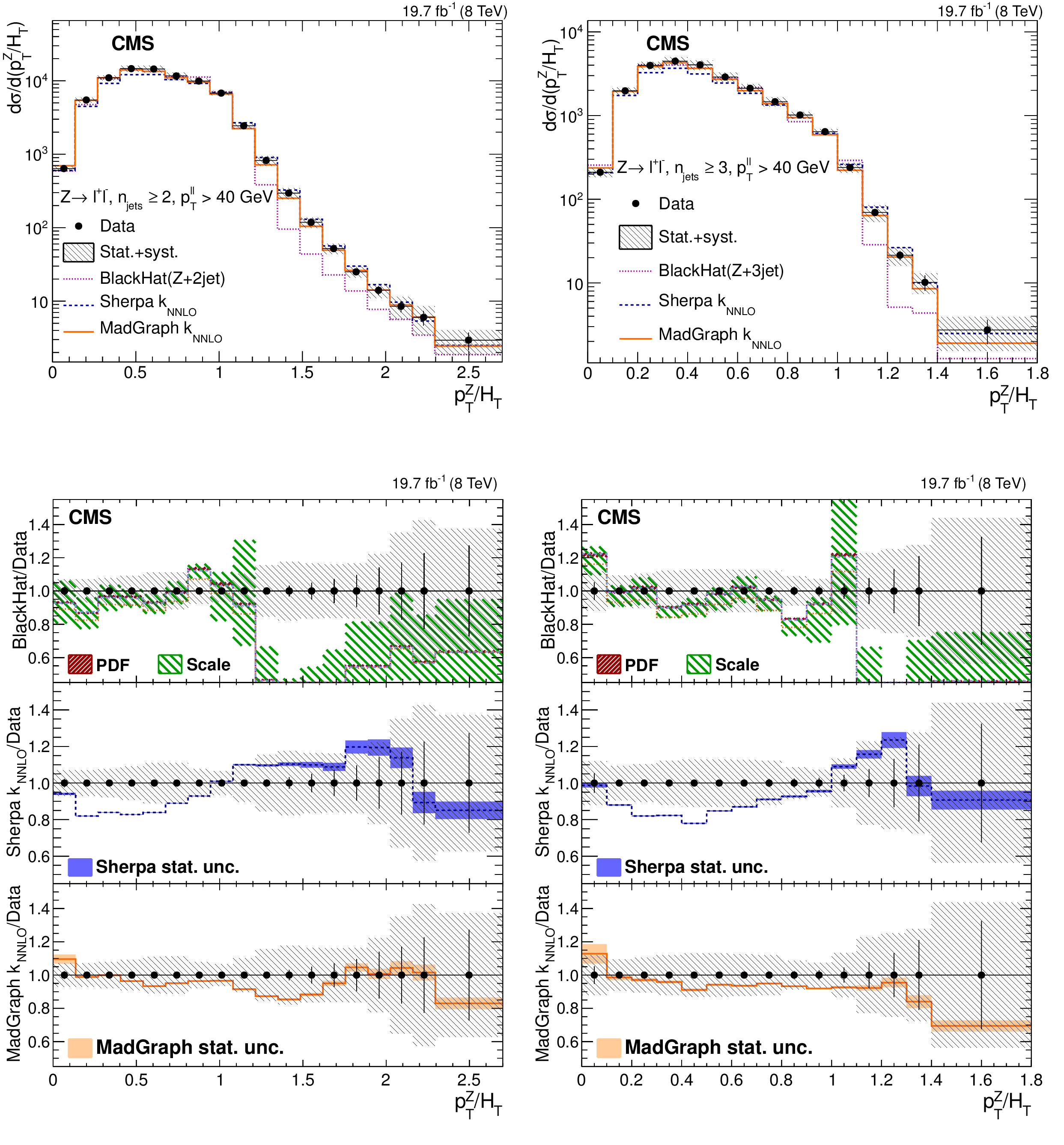
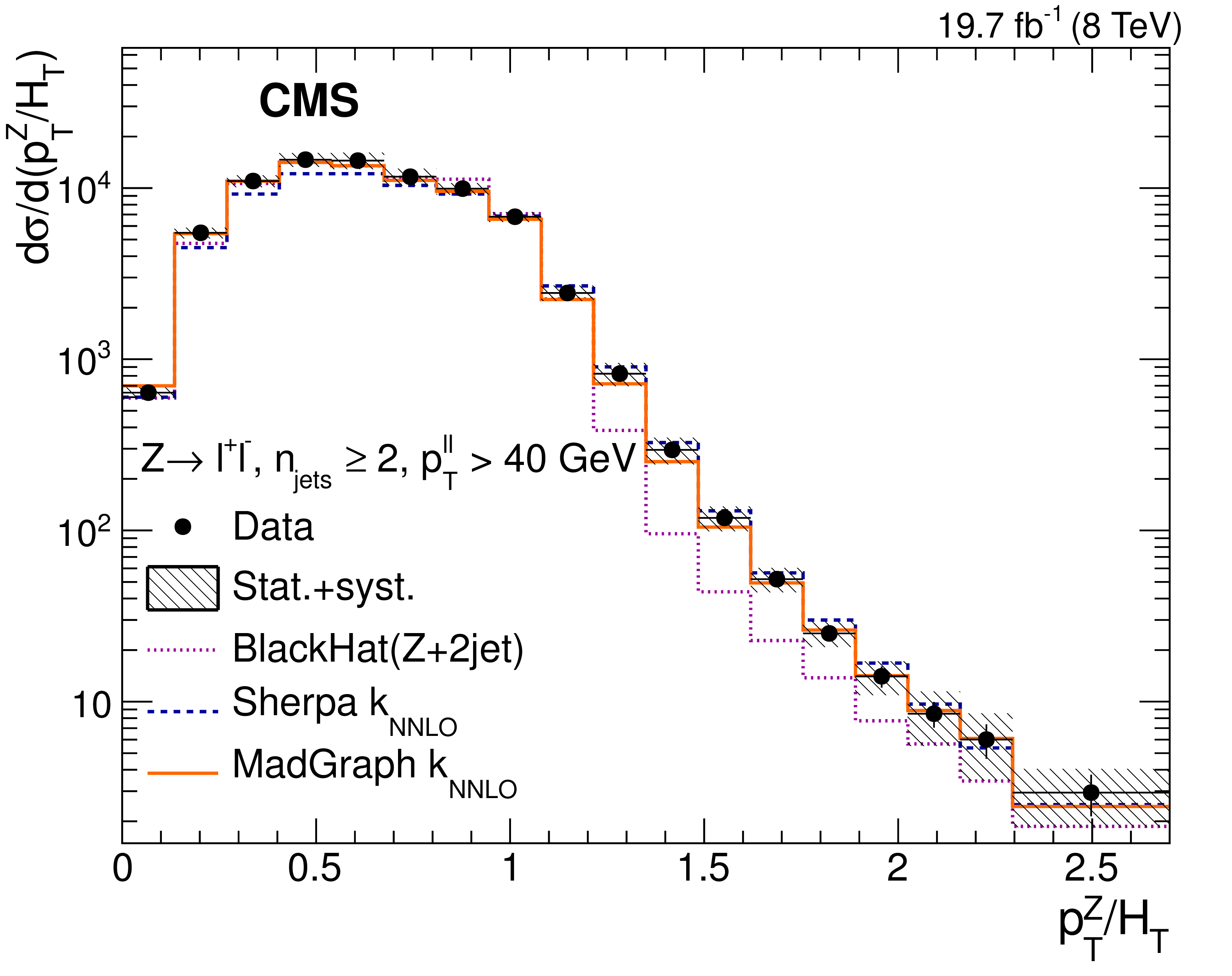
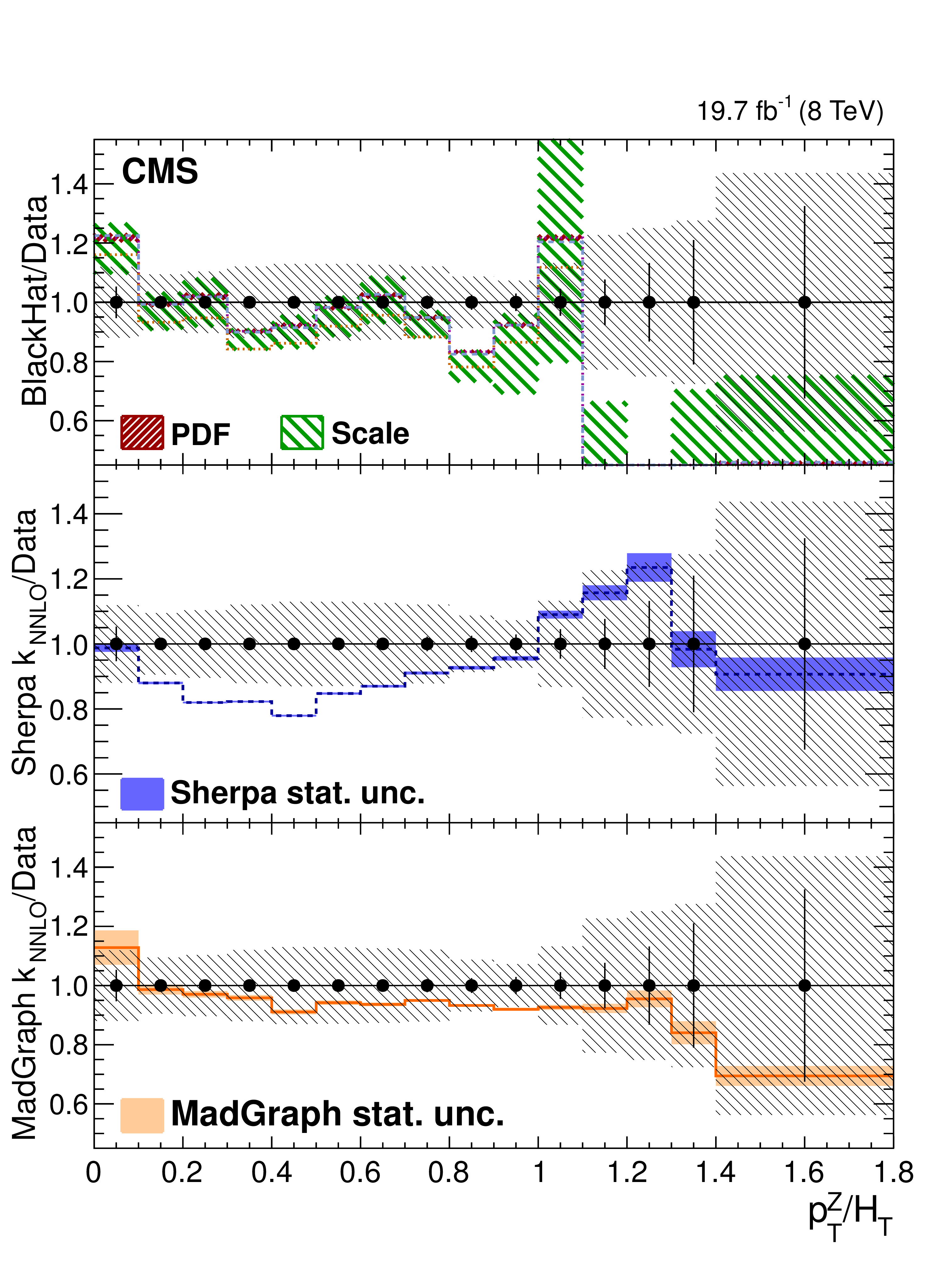
Figure 5:
The measured distribution of the observable $ {p_{\mathrm {T}}} ^{ {\mathrm {Z}}}/ {H_{\mathrm {T}}} $ ratio for $ {n_{\text {jets}}} \geq 2$ (a) and $ {n_{\text {jets}}} \geq 3$ (b) for Z+jets in detector-corrected data compared with estimations from MadGraph+Pythia6, Sherpa, and Blackhat. A detailed explanation is given in the Section on Differential Cross-Sections. The bottom plots give the ratio of the various theoretical estimations to the data in the $ {n_{\text {jets}}} \geq 2$ case (c) and $ {n_{\text {jets}}} \geq 3$ case (d). |
png pdf |
Figure 5-a:
The measured distribution of the observable $ {p_{\mathrm {T}}} ^{ {\mathrm {Z}}}/ {H_{\mathrm {T}}} $ ratio for $ {n_{\text {jets}}} \geq 2$ (a) and $ {n_{\text {jets}}} \geq 3$ (b) for Z+jets in detector-corrected data compared with estimations from MadGraph+Pythia6, Sherpa, and Blackhat. A detailed explanation is given in the Section on Differential Cross-Sections. The bottom plots give the ratio of the various theoretical estimations to the data in the $ {n_{\text {jets}}} \geq 2$ case (c) and $ {n_{\text {jets}}} \geq 3$ case (d). |

png pdf |
Figure 5-b:
The measured distribution of the observable $ {p_{\mathrm {T}}} ^{ {\mathrm {Z}}}/ {H_{\mathrm {T}}} $ ratio for $ {n_{\text {jets}}} \geq 2$ (a) and $ {n_{\text {jets}}} \geq 3$ (b) for Z+jets in detector-corrected data compared with estimations from MadGraph+Pythia6, Sherpa, and Blackhat. A detailed explanation is given in the Section on Differential Cross-Sections. The bottom plots give the ratio of the various theoretical estimations to the data in the $ {n_{\text {jets}}} \geq 2$ case (c) and $ {n_{\text {jets}}} \geq 3$ case (d). |

png pdf |
Figure 5-c:
The measured distribution of the observable $ {p_{\mathrm {T}}} ^{ {\mathrm {Z}}}/ {H_{\mathrm {T}}} $ ratio for $ {n_{\text {jets}}} \geq 2$ (a) and $ {n_{\text {jets}}} \geq 3$ (b) for Z+jets in detector-corrected data compared with estimations from MadGraph+Pythia6, Sherpa, and Blackhat. A detailed explanation is given in the Section on Differential Cross-Sections. The bottom plots give the ratio of the various theoretical estimations to the data in the $ {n_{\text {jets}}} \geq 2$ case (c) and $ {n_{\text {jets}}} \geq 3$ case (d). |
png pdf |
Figure 5-d:
The measured distribution of the observable $ {p_{\mathrm {T}}} ^{ {\mathrm {Z}}}/ {H_{\mathrm {T}}} $ ratio for $ {n_{\text {jets}}} \geq 2$ (a) and $ {n_{\text {jets}}} \geq 3$ (b) for Z+jets in detector-corrected data compared with estimations from MadGraph+Pythia6, Sherpa, and Blackhat. A detailed explanation is given in the Section on Differential Cross-Sections. The bottom plots give the ratio of the various theoretical estimations to the data in the $ {n_{\text {jets}}} \geq 2$ case (c) and $ {n_{\text {jets}}} \geq 3$ case (d). |
png pdf |
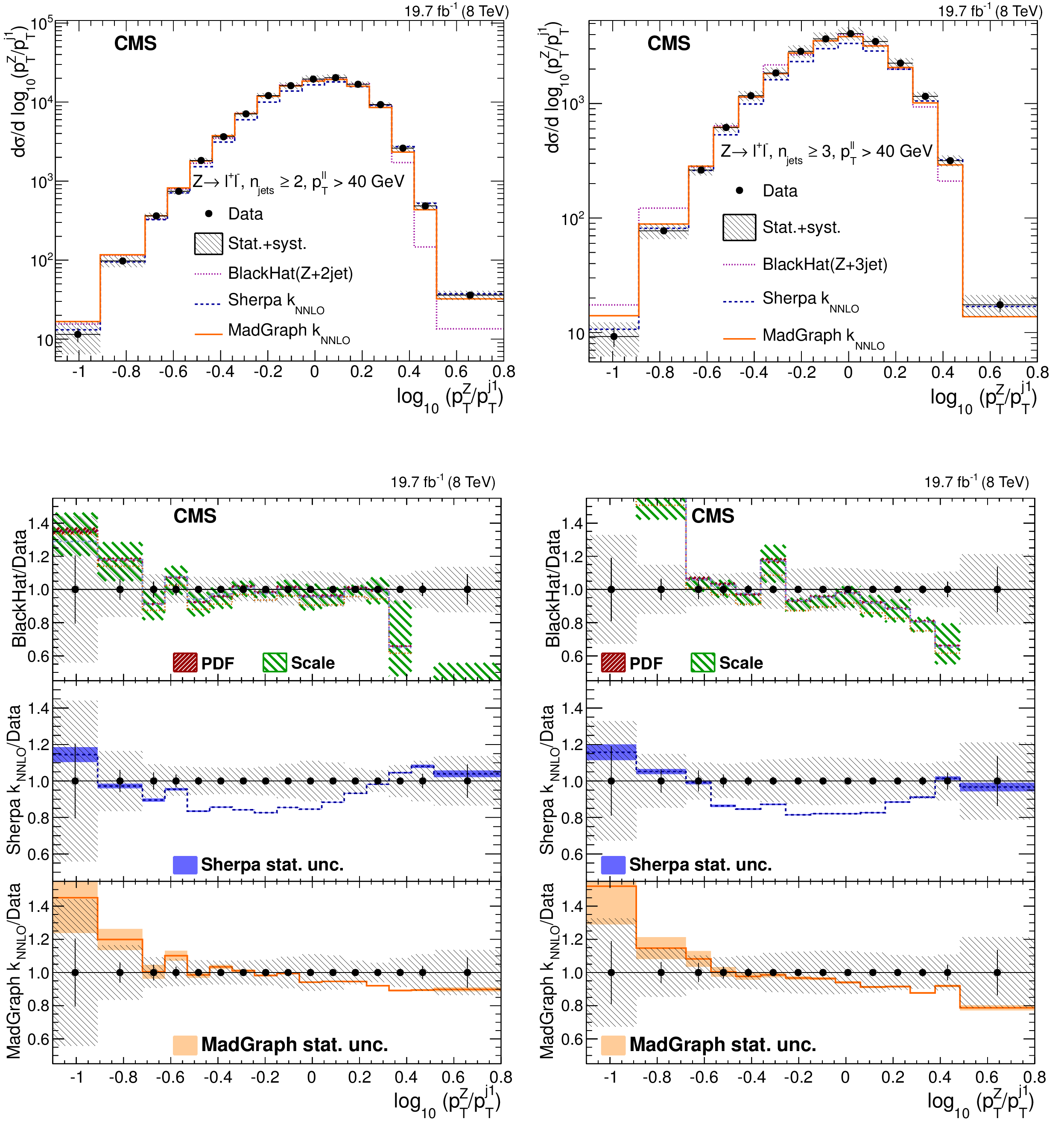
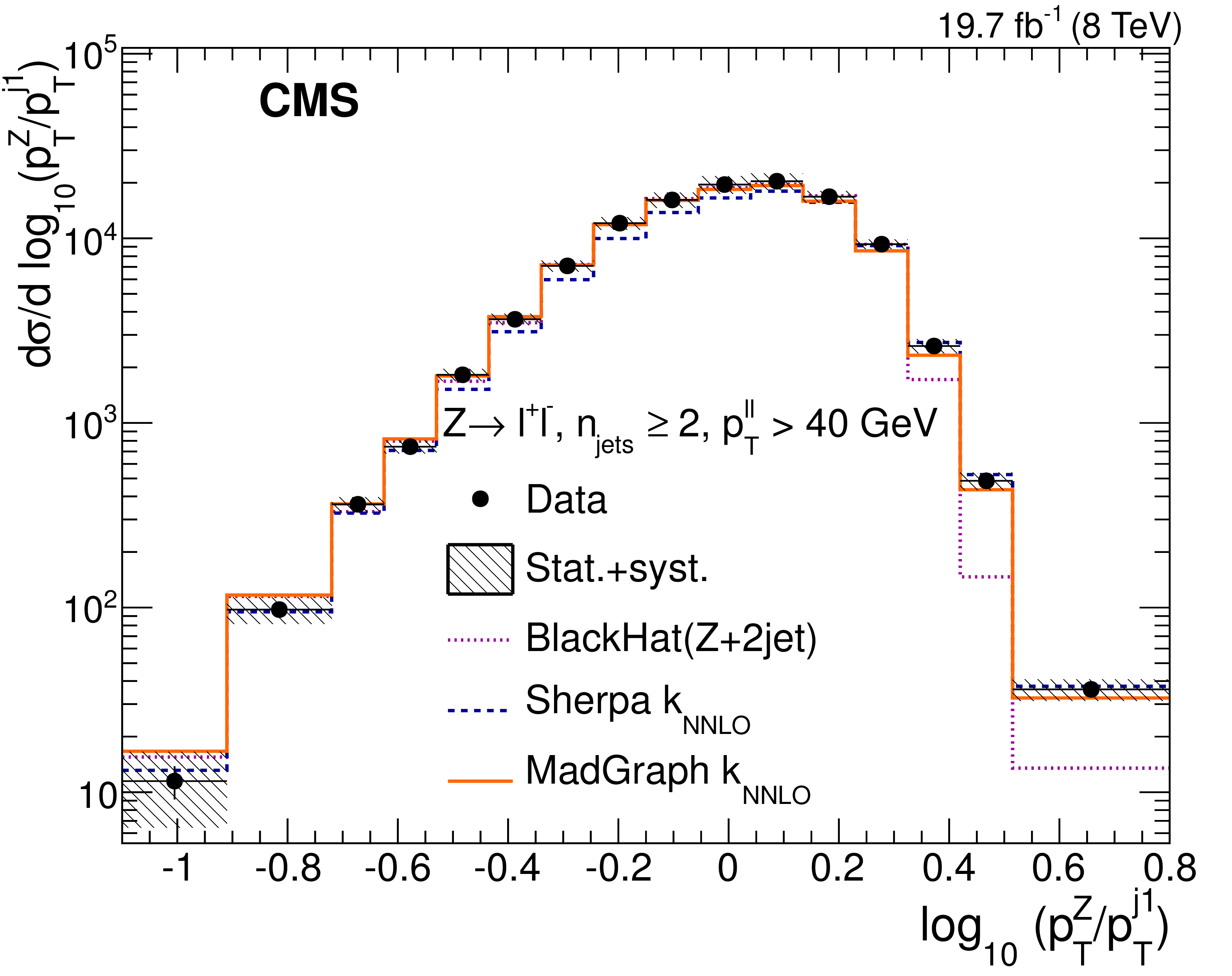
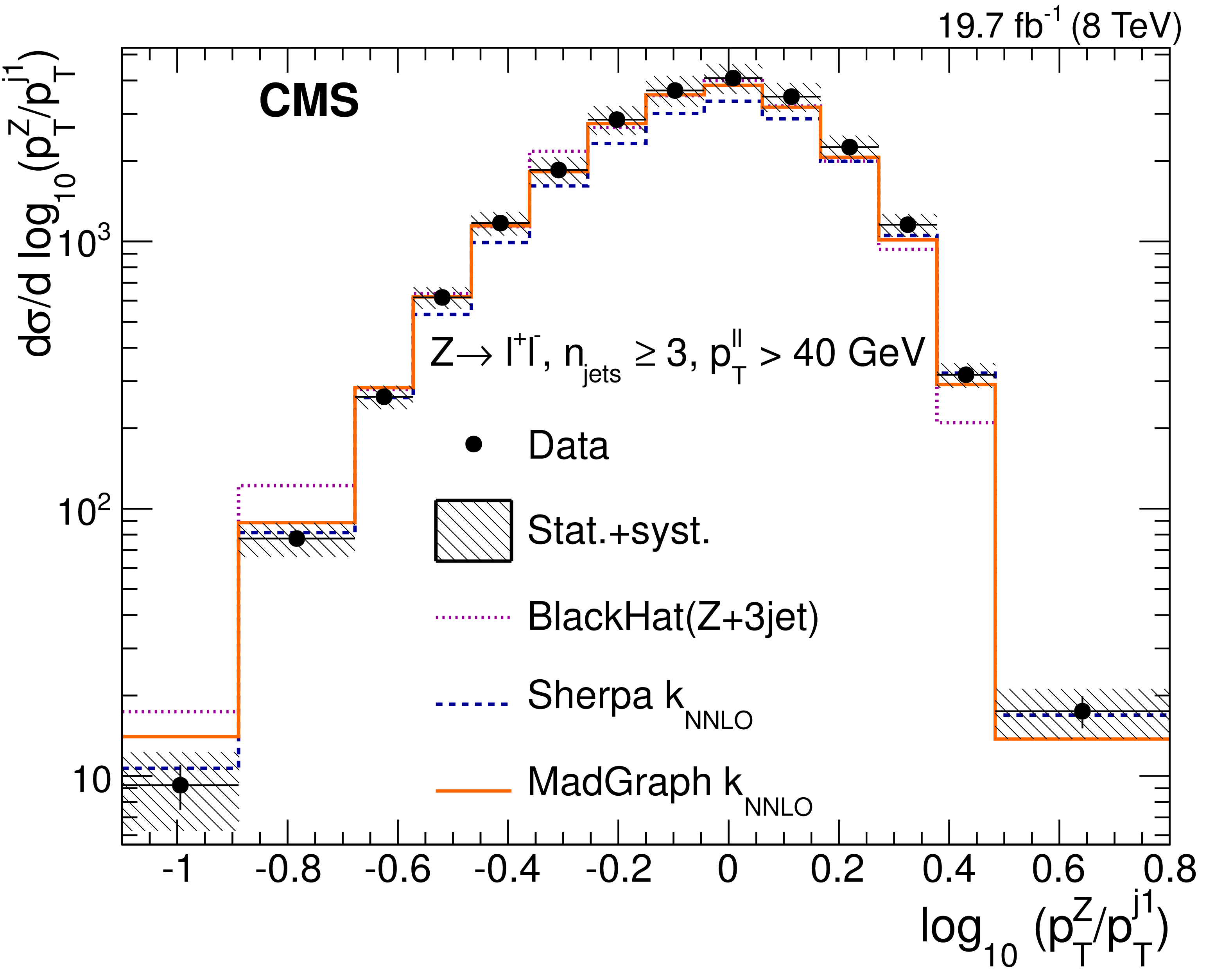
Figure 6:
The measured distribution of the observable $\log_{10} {p_{\mathrm {T}}} ^{ {\mathrm {Z}}}/ {p_{\mathrm {T}}} ^{\mathrm {j}1}$ ratio for $ {n_{\text {jets}}} \geq 2$ (a) and $ {n_{\text {jets}}} \geq 3$ (b) for Z+jets in detector-corrected data compared with estimations from MadGraph+Pythia6, Sherpa, and Blackhat. A detailed explanation is given in the Section on Differential Cross-Sections. The bottom plots give the ratio of the various theoretical estimations to the data in the $ {n_{\text {jets}}} \geq 2$ case (c) and $ {n_{\text {jets}}} \geq 3$ case (d). |
png pdf |
Figure 6-a:
The measured distribution of the observable $\log_{10} {p_{\mathrm {T}}} ^{ {\mathrm {Z}}}/ {p_{\mathrm {T}}} ^{\mathrm {j}1}$ ratio for $ {n_{\text {jets}}} \geq 2$ (a) and $ {n_{\text {jets}}} \geq 3$ (b) for Z+jets in detector-corrected data compared with estimations from MadGraph+Pythia6, Sherpa, and Blackhat. A detailed explanation is given in the Section on Differential Cross-Sections. The bottom plots give the ratio of the various theoretical estimations to the data in the $ {n_{\text {jets}}} \geq 2$ case (c) and $ {n_{\text {jets}}} \geq 3$ case (d). |
png pdf |
Figure 6-b:
The measured distribution of the observable $\log_{10} {p_{\mathrm {T}}} ^{ {\mathrm {Z}}}/ {p_{\mathrm {T}}} ^{\mathrm {j}1}$ ratio for $ {n_{\text {jets}}} \geq 2$ (a) and $ {n_{\text {jets}}} \geq 3$ (b) for Z+jets in detector-corrected data compared with estimations from MadGraph+Pythia6, Sherpa, and Blackhat. A detailed explanation is given in the Section on Differential Cross-Sections. The bottom plots give the ratio of the various theoretical estimations to the data in the $ {n_{\text {jets}}} \geq 2$ case (c) and $ {n_{\text {jets}}} \geq 3$ case (d). |
png pdf |
Figure 6-c:
The measured distribution of the observable $\log_{10} {p_{\mathrm {T}}} ^{ {\mathrm {Z}}}/ {p_{\mathrm {T}}} ^{\mathrm {j}1}$ ratio for $ {n_{\text {jets}}} \geq 2$ (a) and $ {n_{\text {jets}}} \geq 3$ (b) for Z+jets in detector-corrected data compared with estimations from MadGraph+Pythia6, Sherpa, and Blackhat. A detailed explanation is given in the Section on Differential Cross-Sections. The bottom plots give the ratio of the various theoretical estimations to the data in the $ {n_{\text {jets}}} \geq 2$ case (c) and $ {n_{\text {jets}}} \geq 3$ case (d). |
png pdf |
Figure 6-d:
The measured distribution of the observable $\log_{10} {p_{\mathrm {T}}} ^{ {\mathrm {Z}}}/ {p_{\mathrm {T}}} ^{\mathrm {j}1}$ ratio for $ {n_{\text {jets}}} \geq 2$ (a) and $ {n_{\text {jets}}} \geq 3$ (b) for Z+jets in detector-corrected data compared with estimations from MadGraph+Pythia6, Sherpa, and Blackhat. A detailed explanation is given in the Section on Differential Cross-Sections. The bottom plots give the ratio of the various theoretical estimations to the data in the $ {n_{\text {jets}}} \geq 2$ case (c) and $ {n_{\text {jets}}} \geq 3$ case (d). |
png pdf |
Figure 7:
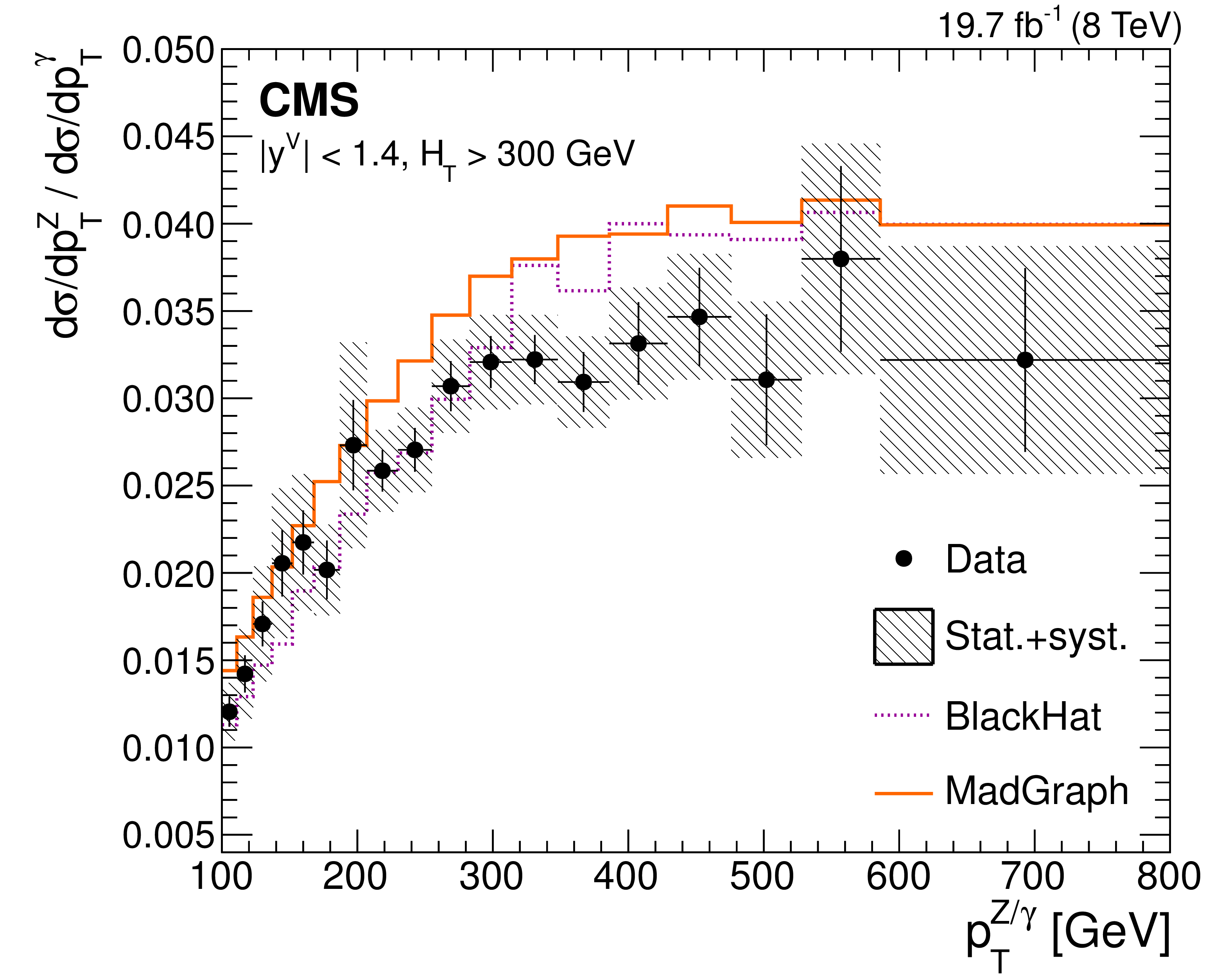
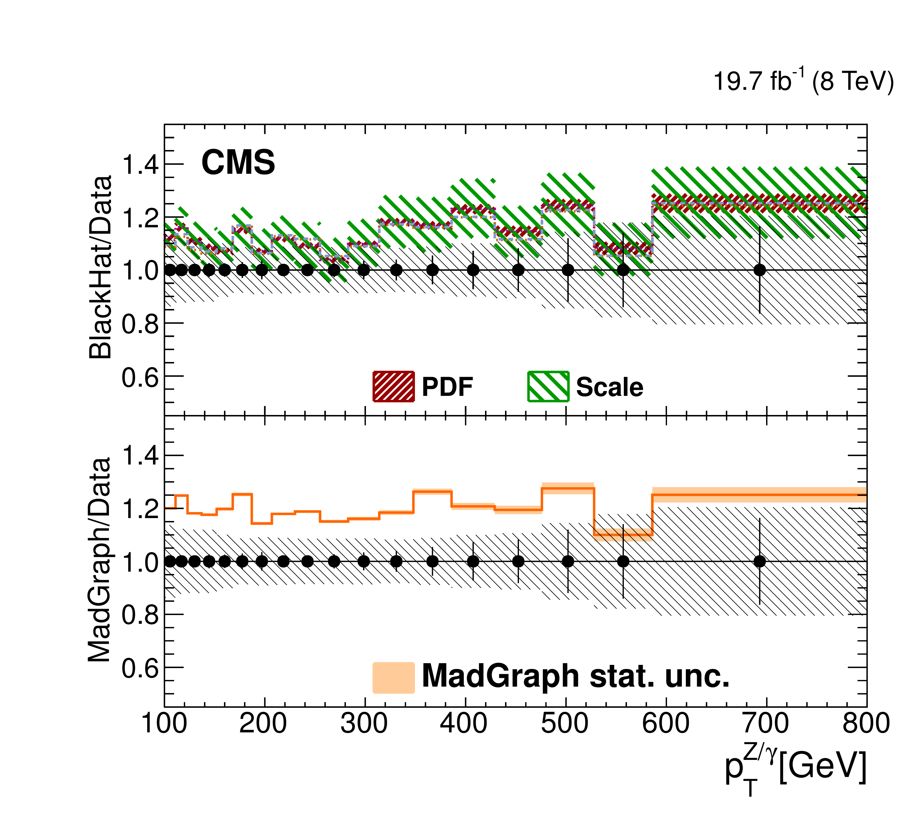
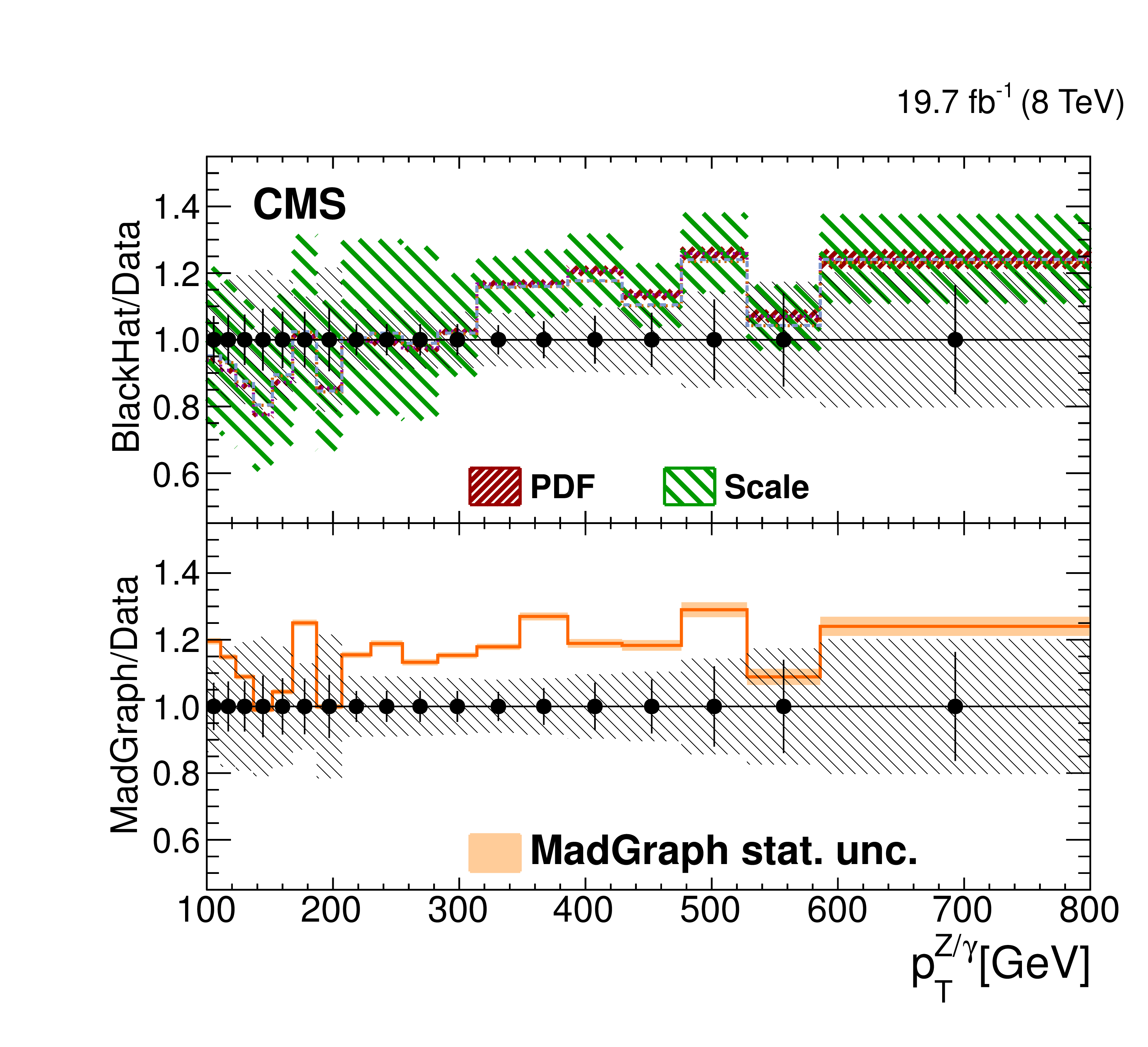
Differential cross section ratio of averaged $ {\mathrm {Z}}\to \left ( {\mathrm {e}^+} {\mathrm {e}^-}+ {\mu ^+} {\mu ^-} \right )$ over $\gamma $ as a function of the total transverse-momentum cross section and for central bosons ($ {| y^{V} | }<1.4$) at different kinematic selections in detector-corrected data. a: inclusive ($ {n_{\text {jets}}} \ge 1$); b: $ {H_{\mathrm {T}}} \ge 300 GeV $, $ {n_{\text {jets}}} \ge 1$. The black error bars reflect the statistical uncertainty in the ratio, the hatched (gray) band represents the total uncertainty in the measurement. The shaded band around the MadGraph+Pythia6 simulation to data ratio represents the statistical uncertainty in the MC estimation. The bottom plots give the ratio of the various theoretical estimations to the data in the $ {n_{\text {jets}}} \geq 1$ case (c) and $ {H_{\mathrm {T}}} \geq 300 GeV $ case (d). |
png pdf |
Figure 7-a:
Differential cross section ratio of averaged $ {\mathrm {Z}}\to \left ( {\mathrm {e}^+} {\mathrm {e}^-}+ {\mu ^+} {\mu ^-} \right )$ over $\gamma $ as a function of the total transverse-momentum cross section and for central bosons ($ {| y^{V} | }<1.4$) at different kinematic selections in detector-corrected data. a: inclusive ($ {n_{\text {jets}}} \ge 1$); b: $ {H_{\mathrm {T}}} \ge 300 GeV $, $ {n_{\text {jets}}} \ge 1$. The black error bars reflect the statistical uncertainty in the ratio, the hatched (gray) band represents the total uncertainty in the measurement. The shaded band around the MadGraph+Pythia6 simulation to data ratio represents the statistical uncertainty in the MC estimation. The bottom plots give the ratio of the various theoretical estimations to the data in the $ {n_{\text {jets}}} \geq 1$ case (c) and $ {H_{\mathrm {T}}} \geq 300 GeV $ case (d). |
png pdf |
Figure 7-b:
Differential cross section ratio of averaged $ {\mathrm {Z}}\to \left ( {\mathrm {e}^+} {\mathrm {e}^-}+ {\mu ^+} {\mu ^-} \right )$ over $\gamma $ as a function of the total transverse-momentum cross section and for central bosons ($ {| y^{V} | }<1.4$) at different kinematic selections in detector-corrected data. a: inclusive ($ {n_{\text {jets}}} \ge 1$); b: $ {H_{\mathrm {T}}} \ge 300 GeV $, $ {n_{\text {jets}}} \ge 1$. The black error bars reflect the statistical uncertainty in the ratio, the hatched (gray) band represents the total uncertainty in the measurement. The shaded band around the MadGraph+Pythia6 simulation to data ratio represents the statistical uncertainty in the MC estimation. The bottom plots give the ratio of the various theoretical estimations to the data in the $ {n_{\text {jets}}} \geq 1$ case (c) and $ {H_{\mathrm {T}}} \geq 300 GeV $ case (d). |
png pdf |
Figure 7-c:
Differential cross section ratio of averaged $ {\mathrm {Z}}\to \left ( {\mathrm {e}^+} {\mathrm {e}^-}+ {\mu ^+} {\mu ^-} \right )$ over $\gamma $ as a function of the total transverse-momentum cross section and for central bosons ($ {| y^{V} | }<1.4$) at different kinematic selections in detector-corrected data. a: inclusive ($ {n_{\text {jets}}} \ge 1$); b: $ {H_{\mathrm {T}}} \ge 300 GeV $, $ {n_{\text {jets}}} \ge 1$. The black error bars reflect the statistical uncertainty in the ratio, the hatched (gray) band represents the total uncertainty in the measurement. The shaded band around the MadGraph+Pythia6 simulation to data ratio represents the statistical uncertainty in the MC estimation. The bottom plots give the ratio of the various theoretical estimations to the data in the $ {n_{\text {jets}}} \geq 1$ case (c) and $ {H_{\mathrm {T}}} \geq 300 GeV $ case (d). |
png pdf |
Figure 7-d:
Differential cross section ratio of averaged $ {\mathrm {Z}}\to \left ( {\mathrm {e}^+} {\mathrm {e}^-}+ {\mu ^+} {\mu ^-} \right )$ over $\gamma $ as a function of the total transverse-momentum cross section and for central bosons ($ {| y^{V} | }<1.4$) at different kinematic selections in detector-corrected data. a: inclusive ($ {n_{\text {jets}}} \ge 1$); b: $ {H_{\mathrm {T}}} \ge 300 GeV $, $ {n_{\text {jets}}} \ge 1$. The black error bars reflect the statistical uncertainty in the ratio, the hatched (gray) band represents the total uncertainty in the measurement. The shaded band around the MadGraph+Pythia6 simulation to data ratio represents the statistical uncertainty in the MC estimation. The bottom plots give the ratio of the various theoretical estimations to the data in the $ {n_{\text {jets}}} \geq 1$ case (c) and $ {H_{\mathrm {T}}} \geq 300 GeV $ case (d). |
png pdf |
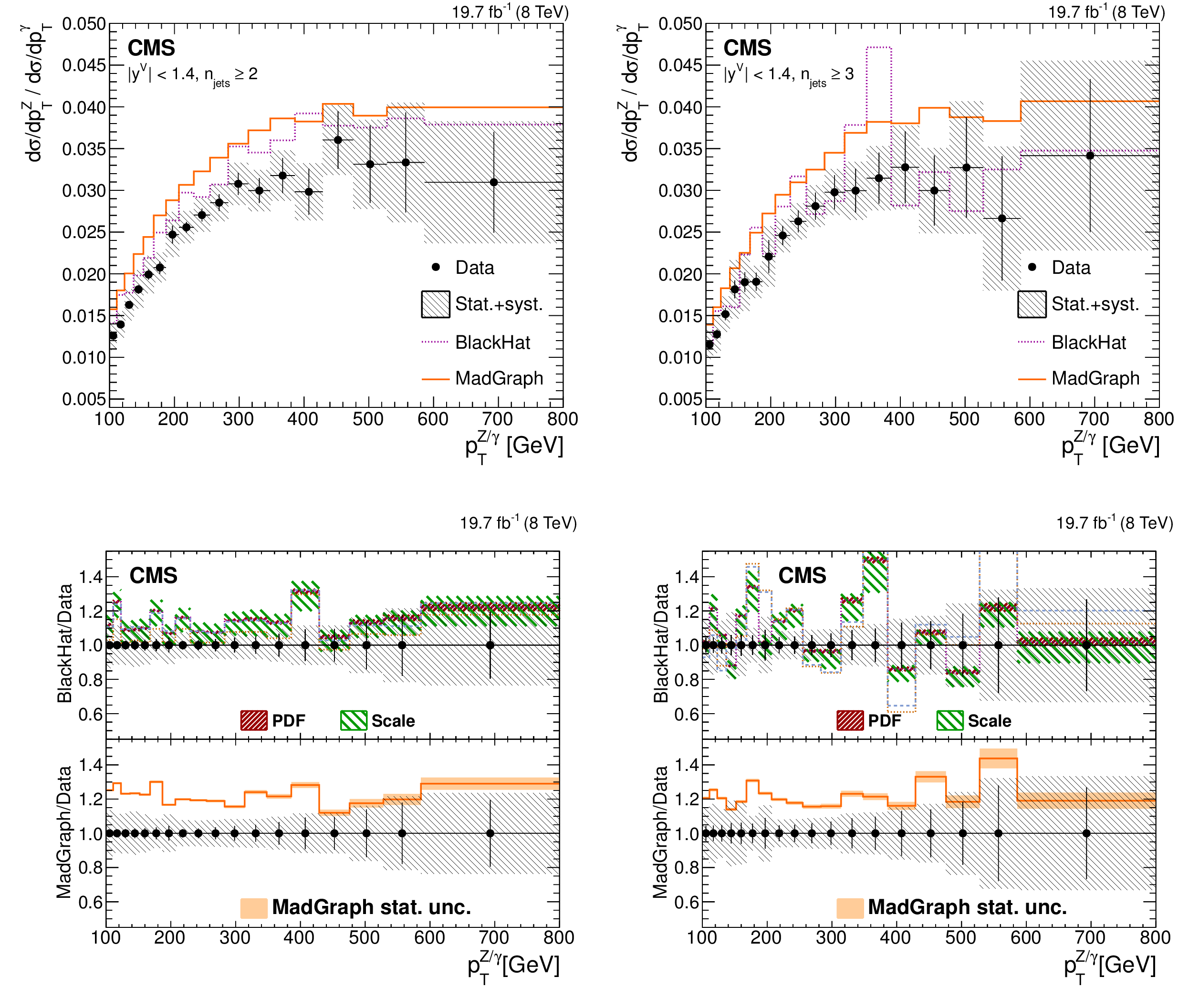
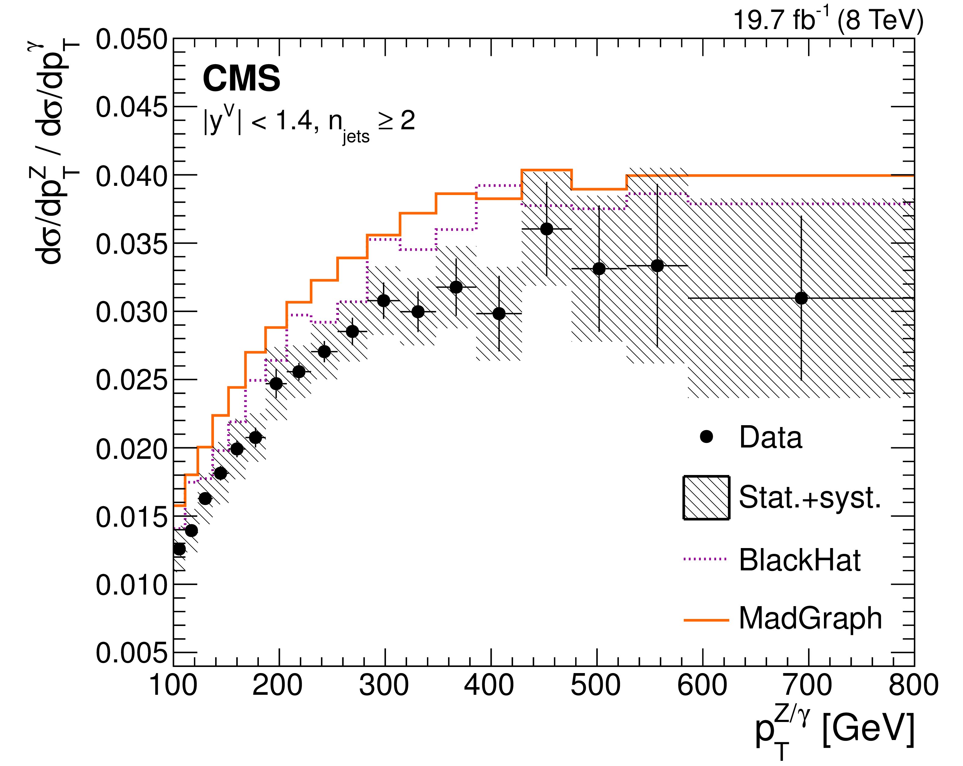
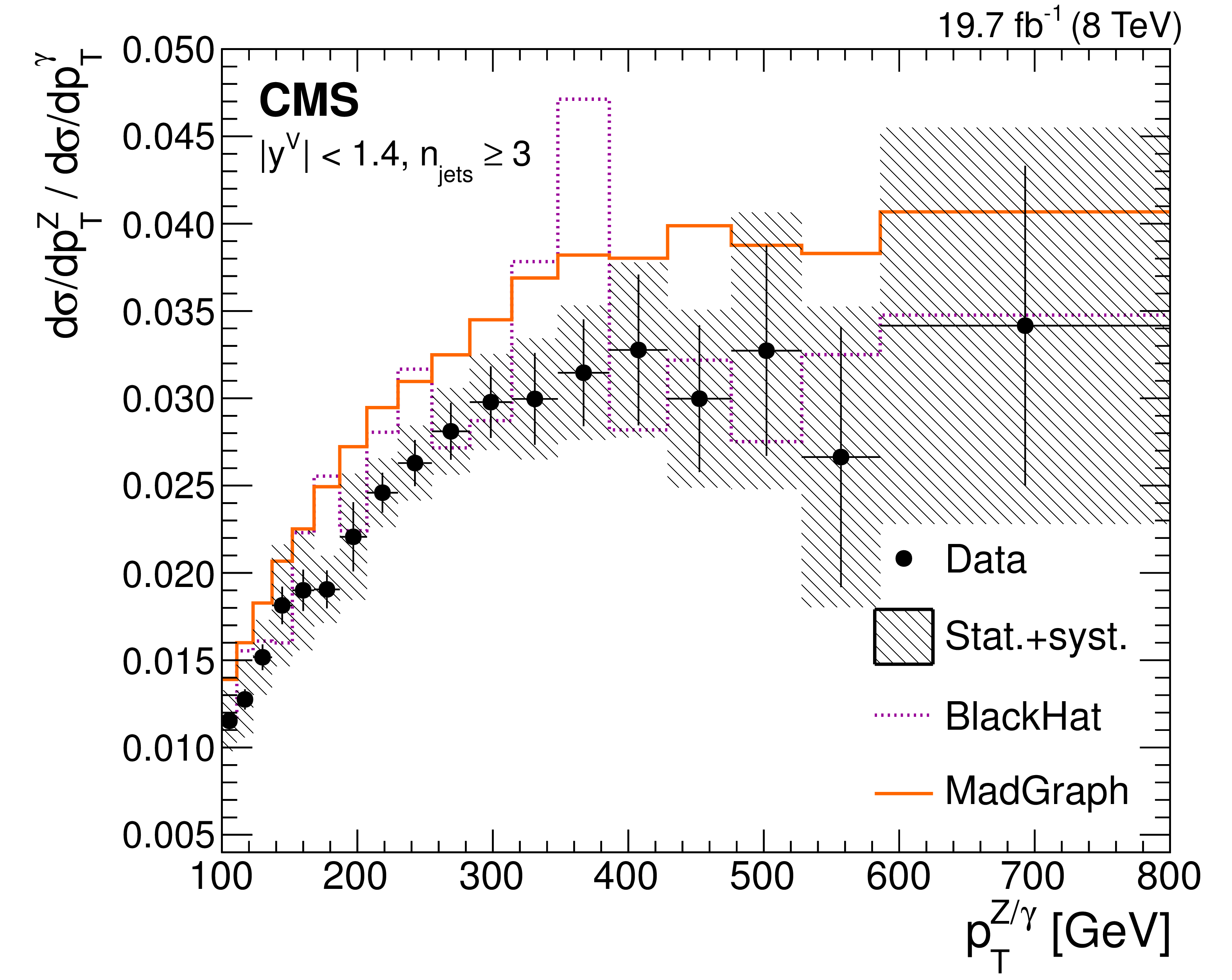
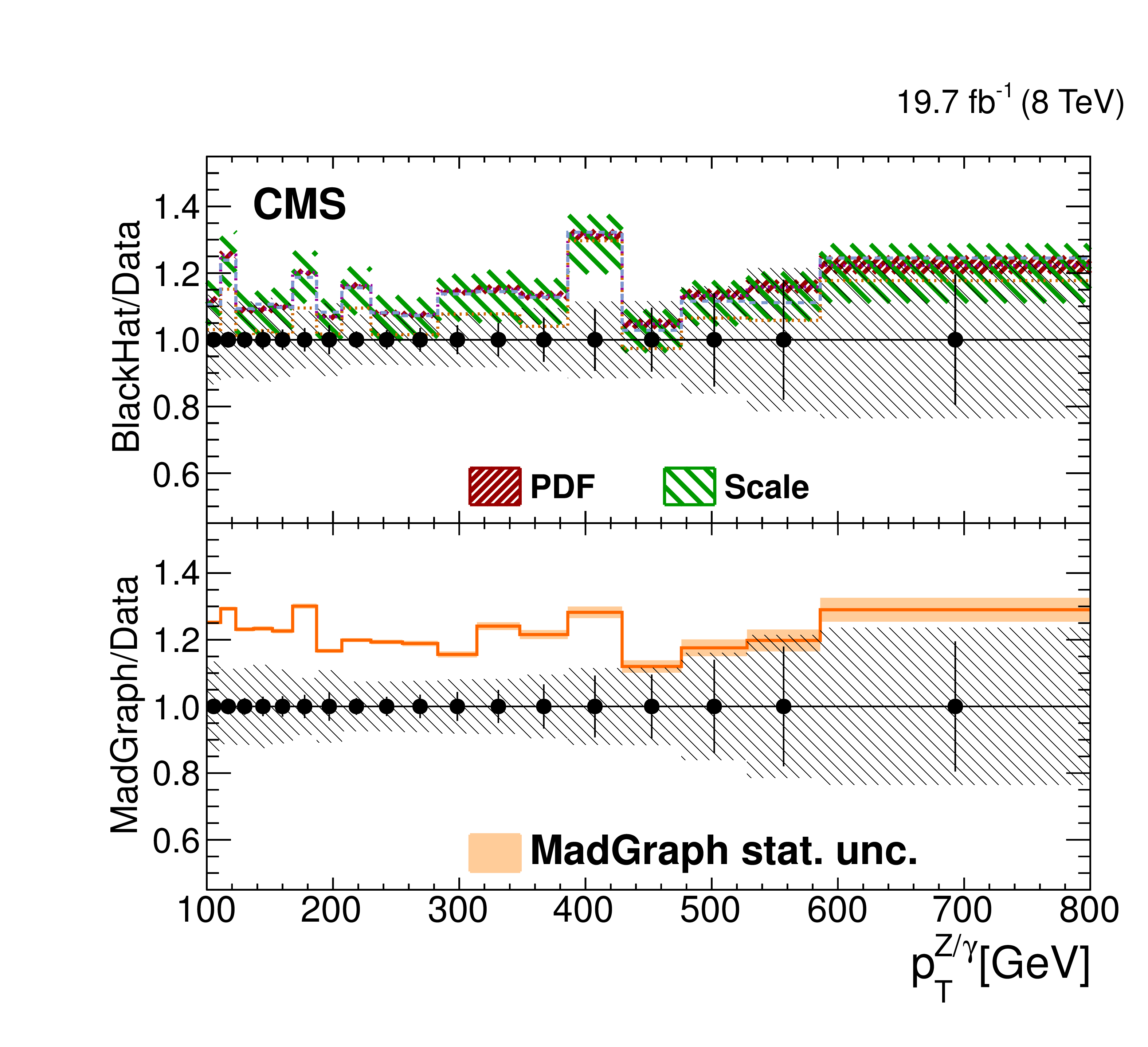
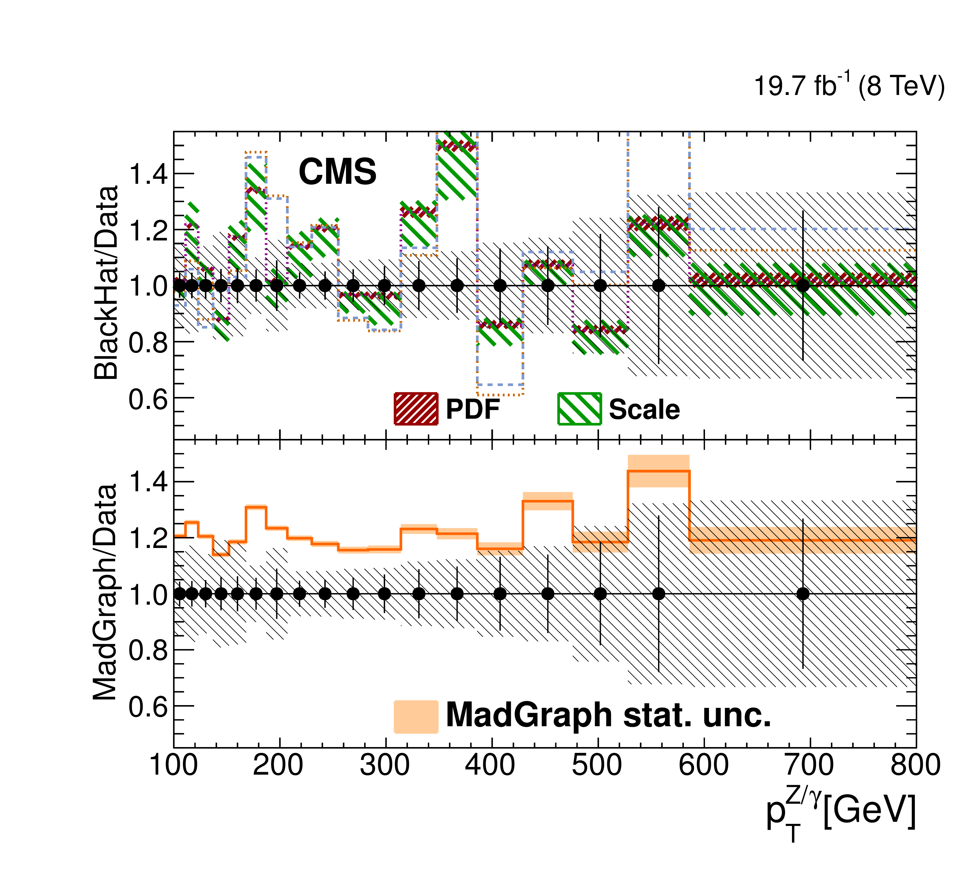
Figure 8:
Differential cross section ratio of $ {\mathrm {Z}}\to \left ( {\mathrm {e}^+} {\mathrm {e}^-}+ {\mu ^+} {\mu ^-} \right )$ over $\gamma $ as a function of the total transverse-momentum cross section and for central bosons ($ {| y^{V} | }<1.4$) at different kinematic selections in detector-corrected data. a: 2-jet ($ {n_{\text {jets}}} \ge 2$); b: 3-jet ($ {n_{\text {jets}}} \ge 3$). The black error bars reflect the statistical uncertainty in the ratio, the hatched (gray) band represents the total uncertainty in the measurement. The shaded band around the MadGraph+Pythia6 simulation to data ratio represents the statistical uncertainty in the MC estimation. The bottom plots give the ratio of the various theoretical estimations to the data in the $ {n_{\text {jets}}} \geq 2$ case (c) and $ {n_{\text {jets}}} \geq 3$ case (d). |
png pdf |
Figure 8-a:
Differential cross section ratio of $ {\mathrm {Z}}\to \left ( {\mathrm {e}^+} {\mathrm {e}^-}+ {\mu ^+} {\mu ^-} \right )$ over $\gamma $ as a function of the total transverse-momentum cross section and for central bosons ($ {| y^{V} | }<1.4$) at different kinematic selections in detector-corrected data. a: 2-jet ($ {n_{\text {jets}}} \ge 2$); b: 3-jet ($ {n_{\text {jets}}} \ge 3$). The black error bars reflect the statistical uncertainty in the ratio, the hatched (gray) band represents the total uncertainty in the measurement. The shaded band around the MadGraph+Pythia6 simulation to data ratio represents the statistical uncertainty in the MC estimation. The bottom plots give the ratio of the various theoretical estimations to the data in the $ {n_{\text {jets}}} \geq 2$ case (c) and $ {n_{\text {jets}}} \geq 3$ case (d). |
png pdf |
Figure 8-b:
Differential cross section ratio of $ {\mathrm {Z}}\to \left ( {\mathrm {e}^+} {\mathrm {e}^-}+ {\mu ^+} {\mu ^-} \right )$ over $\gamma $ as a function of the total transverse-momentum cross section and for central bosons ($ {| y^{V} | }<1.4$) at different kinematic selections in detector-corrected data. a: 2-jet ($ {n_{\text {jets}}} \ge 2$); b: 3-jet ($ {n_{\text {jets}}} \ge 3$). The black error bars reflect the statistical uncertainty in the ratio, the hatched (gray) band represents the total uncertainty in the measurement. The shaded band around the MadGraph+Pythia6 simulation to data ratio represents the statistical uncertainty in the MC estimation. The bottom plots give the ratio of the various theoretical estimations to the data in the $ {n_{\text {jets}}} \geq 2$ case (c) and $ {n_{\text {jets}}} \geq 3$ case (d). |
png pdf |
Figure 8-c:
Differential cross section ratio of $ {\mathrm {Z}}\to \left ( {\mathrm {e}^+} {\mathrm {e}^-}+ {\mu ^+} {\mu ^-} \right )$ over $\gamma $ as a function of the total transverse-momentum cross section and for central bosons ($ {| y^{V} | }<1.4$) at different kinematic selections in detector-corrected data. a: 2-jet ($ {n_{\text {jets}}} \ge 2$); b: 3-jet ($ {n_{\text {jets}}} \ge 3$). The black error bars reflect the statistical uncertainty in the ratio, the hatched (gray) band represents the total uncertainty in the measurement. The shaded band around the MadGraph+Pythia6 simulation to data ratio represents the statistical uncertainty in the MC estimation. The bottom plots give the ratio of the various theoretical estimations to the data in the $ {n_{\text {jets}}} \geq 2$ case (c) and $ {n_{\text {jets}}} \geq 3$ case (d). |
png pdf |
Figure 8-d:
Differential cross section ratio of $ {\mathrm {Z}}\to \left ( {\mathrm {e}^+} {\mathrm {e}^-}+ {\mu ^+} {\mu ^-} \right )$ over $\gamma $ as a function of the total transverse-momentum cross section and for central bosons ($ {| y^{V} | }<1.4$) at different kinematic selections in detector-corrected data. a: 2-jet ($ {n_{\text {jets}}} \ge 2$); b: 3-jet ($ {n_{\text {jets}}} \ge 3$). The black error bars reflect the statistical uncertainty in the ratio, the hatched (gray) band represents the total uncertainty in the measurement. The shaded band around the MadGraph+Pythia6 simulation to data ratio represents the statistical uncertainty in the MC estimation. The bottom plots give the ratio of the various theoretical estimations to the data in the $ {n_{\text {jets}}} \geq 2$ case (c) and $ {n_{\text {jets}}} \geq 3$ case (d). |
| Tables | |
png pdf |
Table 1:
Systematic uncertainties for the $ { {p_{\mathrm {T}}} ^{ {\mathrm {Z}}}} $ spectrum. |
png pdf |
Table 2:
Systematic uncertainties for the $ { {p_{\mathrm {T}}} ^{\gamma }} $ spectrum. |
| Summary |
| Differential cross sections have been measured for Z+jets (with Z $\to \ell^+\ell^-$) and isolated $\gamma$+jets as a function of the boson transverse momentum, using data collected by CMS at $\sqrt{s} =$ 8 TeV corresponding to an integrated luminosity of 19.7 fb$^{-1}$. The estimations from the MC multiparton LO+PS generators MADGRAPH+PYTHIA6 and SHERPA have been compared to the data. We find that the $p_{\mathrm{T}}$ spectra for Z+jets and $\gamma$+jets are not well reproduced by these MC models. We observe a monotonic increase of the MC simulation/data ratio with increasing vector boson $p_{\mathrm{T}}$. Using the NLO generator BLACKHAT simulation, we find a smaller discrepancy in shape between data and simulation, indicating that it is likely related to missing higher-order effects. We have also studied the distribution of the ratios of $p_{\mathrm{T}}^{\mathrm{Z}}$ and hadronic quantities ($H_{\mathrm{T}}$ and $p_{\mathrm{T}}^{j1}$) in Z+jets. We find that these agree with the LO+PS estimation over the whole range when an NNLO K-factor is applied. The NLO BLACKHAT estimation is accurate in a subrange where the NLO estimation is expected to perform well. In addition, we presented a measurement of the ratio of the Z+jets to $\gamma$+jets cross sections in four phase space regions: $n_{\text{jets}} \ge$ 1, 2, 3, and $H_{\mathrm{T}} >$ 300 GeV, $n_{\text{jets}} \ge$ 1. MADGRAPH+PYTHIA6 (LO+PS) overestimates the data by a factor 1.21 $\pm$ 0.08 (stat+syst), whereas BLACKHAT (NLO) overestimates the data by a factor 1.18 $\pm$ 0.14 (stat+syst). As a function of the vector boson transverse momentum, these factors are at similar values of around 1.2 for all the considered phase space selections. Thus, we find that simulations reproduce the shape of the ratio of $p_{\mathrm{T}}^{\mathrm{Z}}$ to $p_{\mathrm{T}}^{\gamma}$ distributions better than the individual $p_{\mathrm{T}}^{\mathrm{Z}}$ or $p_{\mathrm{T}}^{\gamma}$ distributions in all selections considered. These four selections mimic phase space regions of interest for searches of physics beyond the standard model. We emphasize that the agreement is similar for different jet multiplicities and $H_{\mathrm{T}}$ ranges because Z+jets and $\gamma$+jets events have been generated with the same level of accuracy for up to four partons in the final-state ME. In the comparison, we considered both processes at either LO or at NLO. It is clear from the differences observed between the NLO and LO+PS estimations in each process, the conclusions may not be true if the samples are generated with different orders of accuracies of the matrix element calculation. Our results show that properties of the Z $\to \nu\nu$ process can be predicted using the measured $\gamma$+jets final state and the simulated ratio between Z $\to \nu\nu$+jets and $\gamma$+jets. However, this simulated ratio must be corrected with the measured ratio of leptonic Z+jets and $\gamma$+jets. |
| Additional Figures | |
png pdf |
Additional Figure 4-a:
a,c: The Z boson differential transverse momentum cross-section in an inclusive $Z/\gamma^{*}+\mathrm{jets}$, $N_{\mathrm{jets}} \geq3$ selection in data compared with predictions from MadGraph5.1.3.30+Pythia6.4.26, Sherpa1.4.2 and BlackHat+Sherpa. b,d: the $\gamma$ differential transverse momentum cross-section in an inclusive $\gamma+\mathrm{jets}$, $N_{\mathrm{jets}} \geq3$ selection for central rapidities $| y_{\gamma} | < $ 1.4 in data compared with predictions from MadGraph5.1.3.30+Pythia6.4.26 and BlackHat+Sherpa. For the $Z/\gamma^{*}+\mathrm{jets}$, MadGraph and Sherpa are scaled by a global NNLO k-Factor, for $\gamma+\mathrm{jets}$, the LO cross-section from MadGraph is used. The hatched (grey) band represents the total uncertainty on the measurement, while the error bars show the statistical uncertainty. The shaded bands around MC/data ratios of MadGraph and Sherpa represent the statistical uncertainty of the MC prediction. The (green) hatched band around BlackHat/data ratio (using MSTW) represents the total uncertainty of the prediction due to PDF and scale variations, while the inner (dark red) hatched band the uncertainty due to PDF variations. Overlaid in dashed blue and orange are BlackHat predictions using the NNPDF2.3 and CT10 PDF sets, respectively. |

png pdf |
Additional Figure 4-b:
a,c: The Z boson differential transverse momentum cross-section in an inclusive $Z/\gamma^{*}+\mathrm{jets}$, $N_{\mathrm{jets}} \geq3$ selection in data compared with predictions from MadGraph5.1.3.30+Pythia6.4.26, Sherpa1.4.2 and BlackHat+Sherpa. b,d: the $\gamma$ differential transverse momentum cross-section in an inclusive $\gamma+\mathrm{jets}$, $N_{\mathrm{jets}} \geq3$ selection for central rapidities $| y_{\gamma} | < $ 1.4 in data compared with predictions from MadGraph5.1.3.30+Pythia6.4.26 and BlackHat+Sherpa. For the $Z/\gamma^{*}+\mathrm{jets}$, MadGraph and Sherpa are scaled by a global NNLO k-Factor, for $\gamma+\mathrm{jets}$, the LO cross-section from MadGraph is used. The hatched (grey) band represents the total uncertainty on the measurement, while the error bars show the statistical uncertainty. The shaded bands around MC/data ratios of MadGraph and Sherpa represent the statistical uncertainty of the MC prediction. The (green) hatched band around BlackHat/data ratio (using MSTW) represents the total uncertainty of the prediction due to PDF and scale variations, while the inner (dark red) hatched band the uncertainty due to PDF variations. Overlaid in dashed blue and orange are BlackHat predictions using the NNPDF2.3 and CT10 PDF sets, respectively. |

png pdf |
Additional Figure 4-c:
a,c: The Z boson differential transverse momentum cross-section in an inclusive $Z/\gamma^{*}+\mathrm{jets}$, $N_{\mathrm{jets}} \geq3$ selection in data compared with predictions from MadGraph5.1.3.30+Pythia6.4.26, Sherpa1.4.2 and BlackHat+Sherpa. b,d: the $\gamma$ differential transverse momentum cross-section in an inclusive $\gamma+\mathrm{jets}$, $N_{\mathrm{jets}} \geq3$ selection for central rapidities $| y_{\gamma} | < $ 1.4 in data compared with predictions from MadGraph5.1.3.30+Pythia6.4.26 and BlackHat+Sherpa. For the $Z/\gamma^{*}+\mathrm{jets}$, MadGraph and Sherpa are scaled by a global NNLO k-Factor, for $\gamma+\mathrm{jets}$, the LO cross-section from MadGraph is used. The hatched (grey) band represents the total uncertainty on the measurement, while the error bars show the statistical uncertainty. The shaded bands around MC/data ratios of MadGraph and Sherpa represent the statistical uncertainty of the MC prediction. The (green) hatched band around BlackHat/data ratio (using MSTW) represents the total uncertainty of the prediction due to PDF and scale variations, while the inner (dark red) hatched band the uncertainty due to PDF variations. Overlaid in dashed blue and orange are BlackHat predictions using the NNPDF2.3 and CT10 PDF sets, respectively. |
png pdf |
Additional Figure 4-d:
a,c: The Z boson differential transverse momentum cross-section in an inclusive $Z/\gamma^{*}+\mathrm{jets}$, $N_{\mathrm{jets}} \geq3$ selection in data compared with predictions from MadGraph5.1.3.30+Pythia6.4.26, Sherpa1.4.2 and BlackHat+Sherpa. b,d: the $\gamma$ differential transverse momentum cross-section in an inclusive $\gamma+\mathrm{jets}$, $N_{\mathrm{jets}} \geq3$ selection for central rapidities $| y_{\gamma} | < $ 1.4 in data compared with predictions from MadGraph5.1.3.30+Pythia6.4.26 and BlackHat+Sherpa. For the $Z/\gamma^{*}+\mathrm{jets}$, MadGraph and Sherpa are scaled by a global NNLO k-Factor, for $\gamma+\mathrm{jets}$, the LO cross-section from MadGraph is used. The hatched (grey) band represents the total uncertainty on the measurement, while the error bars show the statistical uncertainty. The shaded bands around MC/data ratios of MadGraph and Sherpa represent the statistical uncertainty of the MC prediction. The (green) hatched band around BlackHat/data ratio (using MSTW) represents the total uncertainty of the prediction due to PDF and scale variations, while the inner (dark red) hatched band the uncertainty due to PDF variations. Overlaid in dashed blue and orange are BlackHat predictions using the NNPDF2.3 and CT10 PDF sets, respectively. |

png pdf |
Additional Figure 5-a:
a,c: The Z boson differential transverse momentum cross-section in an inclusive $Z/\gamma^{*}+\mathrm{jets}$, $N_{\mathrm{jets}} \geq1$, $H_{\mathrm{T}} > $ 300 GeV selection in data compared with predictions from MadGraph5.1.3.30+Pythia6.4.26, Sherpa1.4.2 and BlackHat+Sherpa. b,d: the $\gamma$ differential transverse momentum cross-section in an inclusive $\gamma+\mathrm{jets}$, $N_{\mathrm{jets}} \geq1$, $H_{\mathrm{T}} >$ 300 GeV selection for central rapidities $| y_{\gamma} | <$ 1.4 in data compared with predictions from MadGraph5.1.3.30+Pythia6.4.26 and BlackHat+Sherpa. For the $Z/\gamma^{*}+\mathrm{jets}$, MadGraph and Sherpa are scaled by a global NNLO k-Factor, for $\gamma+\mathrm{jets}$, the LO cross-section from MadGraph is used. The hatched (grey) band represents the total uncertainty on the measurement, while the error bars show the statistical uncertainty. The shaded bands around MC/data ratios of MadGraph and Sherpa represent the statistical uncertainty of the MC prediction. The (green) hatched band around BlackHat/data ratio (using MSTW) represents the total uncertainty of the prediction due to PDF and scale variations, while the inner (dark red) hatched band the uncertainty due to PDF variations. Overlaid in dashed blue and orange are BlackHat predictions using the NNPDF2.3 and CT10 PDF sets, respectively. |
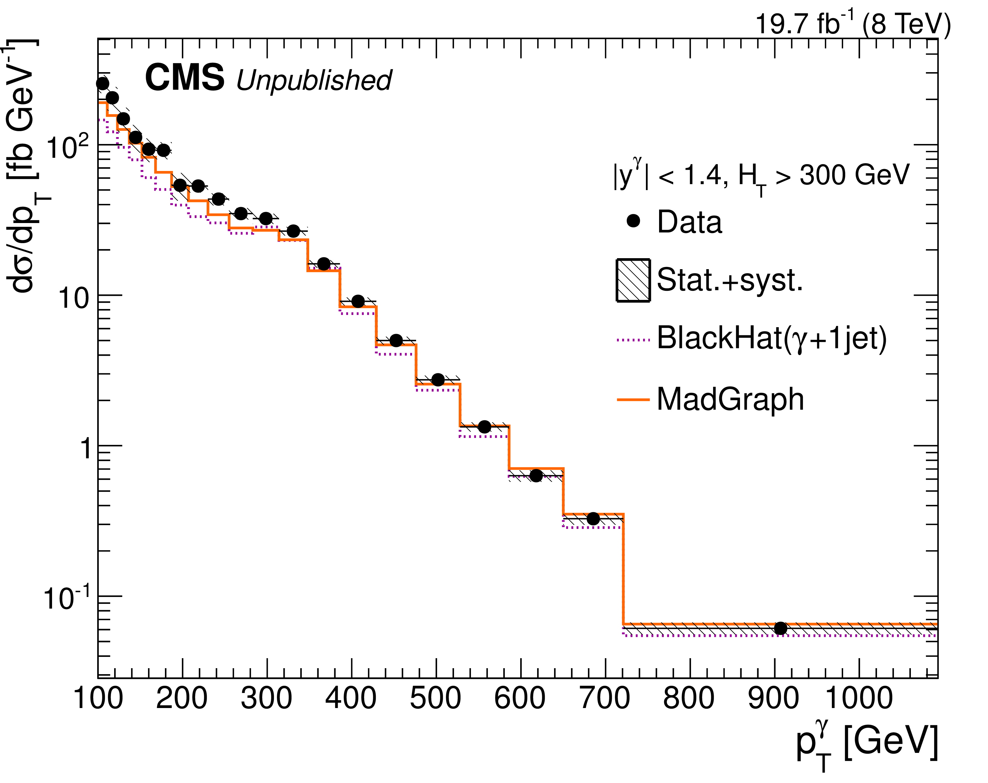
png pdf |
Additional Figure 5-b:
a,c: The Z boson differential transverse momentum cross-section in an inclusive $Z/\gamma^{*}+\mathrm{jets}$, $N_{\mathrm{jets}} \geq1$, $H_{\mathrm{T}} > $ 300 GeV selection in data compared with predictions from MadGraph5.1.3.30+Pythia6.4.26, Sherpa1.4.2 and BlackHat+Sherpa. b,d: the $\gamma$ differential transverse momentum cross-section in an inclusive $\gamma+\mathrm{jets}$, $N_{\mathrm{jets}} \geq1$, $H_{\mathrm{T}} >$ 300 GeV selection for central rapidities $| y_{\gamma} | <$ 1.4 in data compared with predictions from MadGraph5.1.3.30+Pythia6.4.26 and BlackHat+Sherpa. For the $Z/\gamma^{*}+\mathrm{jets}$, MadGraph and Sherpa are scaled by a global NNLO k-Factor, for $\gamma+\mathrm{jets}$, the LO cross-section from MadGraph is used. The hatched (grey) band represents the total uncertainty on the measurement, while the error bars show the statistical uncertainty. The shaded bands around MC/data ratios of MadGraph and Sherpa represent the statistical uncertainty of the MC prediction. The (green) hatched band around BlackHat/data ratio (using MSTW) represents the total uncertainty of the prediction due to PDF and scale variations, while the inner (dark red) hatched band the uncertainty due to PDF variations. Overlaid in dashed blue and orange are BlackHat predictions using the NNPDF2.3 and CT10 PDF sets, respectively. |

png pdf |
Additional Figure 5-c:
a,c: The Z boson differential transverse momentum cross-section in an inclusive $Z/\gamma^{*}+\mathrm{jets}$, $N_{\mathrm{jets}} \geq1$, $H_{\mathrm{T}} > $ 300 GeV selection in data compared with predictions from MadGraph5.1.3.30+Pythia6.4.26, Sherpa1.4.2 and BlackHat+Sherpa. b,d: the $\gamma$ differential transverse momentum cross-section in an inclusive $\gamma+\mathrm{jets}$, $N_{\mathrm{jets}} \geq1$, $H_{\mathrm{T}} >$ 300 GeV selection for central rapidities $| y_{\gamma} | <$ 1.4 in data compared with predictions from MadGraph5.1.3.30+Pythia6.4.26 and BlackHat+Sherpa. For the $Z/\gamma^{*}+\mathrm{jets}$, MadGraph and Sherpa are scaled by a global NNLO k-Factor, for $\gamma+\mathrm{jets}$, the LO cross-section from MadGraph is used. The hatched (grey) band represents the total uncertainty on the measurement, while the error bars show the statistical uncertainty. The shaded bands around MC/data ratios of MadGraph and Sherpa represent the statistical uncertainty of the MC prediction. The (green) hatched band around BlackHat/data ratio (using MSTW) represents the total uncertainty of the prediction due to PDF and scale variations, while the inner (dark red) hatched band the uncertainty due to PDF variations. Overlaid in dashed blue and orange are BlackHat predictions using the NNPDF2.3 and CT10 PDF sets, respectively. |
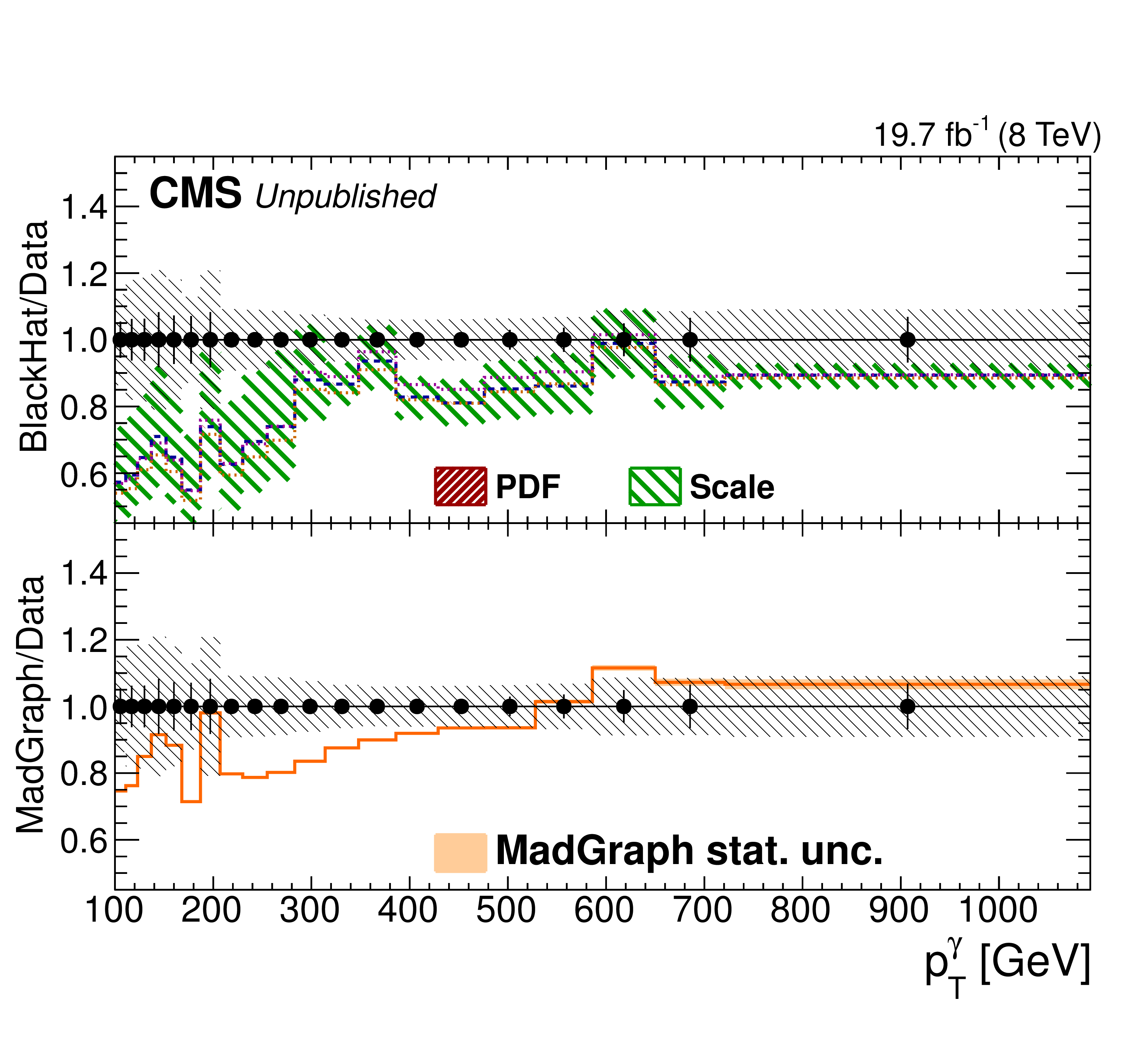
png pdf |
Additional Figure 5-d:
a,c: The Z boson differential transverse momentum cross-section in an inclusive $Z/\gamma^{*}+\mathrm{jets}$, $N_{\mathrm{jets}} \geq1$, $H_{\mathrm{T}} > $ 300 GeV selection in data compared with predictions from MadGraph5.1.3.30+Pythia6.4.26, Sherpa1.4.2 and BlackHat+Sherpa. b,d: the $\gamma$ differential transverse momentum cross-section in an inclusive $\gamma+\mathrm{jets}$, $N_{\mathrm{jets}} \geq1$, $H_{\mathrm{T}} >$ 300 GeV selection for central rapidities $| y_{\gamma} | <$ 1.4 in data compared with predictions from MadGraph5.1.3.30+Pythia6.4.26 and BlackHat+Sherpa. For the $Z/\gamma^{*}+\mathrm{jets}$, MadGraph and Sherpa are scaled by a global NNLO k-Factor, for $\gamma+\mathrm{jets}$, the LO cross-section from MadGraph is used. The hatched (grey) band represents the total uncertainty on the measurement, while the error bars show the statistical uncertainty. The shaded bands around MC/data ratios of MadGraph and Sherpa represent the statistical uncertainty of the MC prediction. The (green) hatched band around BlackHat/data ratio (using MSTW) represents the total uncertainty of the prediction due to PDF and scale variations, while the inner (dark red) hatched band the uncertainty due to PDF variations. Overlaid in dashed blue and orange are BlackHat predictions using the NNPDF2.3 and CT10 PDF sets, respectively. |
|
|
Compact Muon Solenoid LHC, CERN |
|

|

|

|

|

|