

Compact Muon Solenoid
LHC, CERN
| CMS-SUS-14-014 ; CERN-PH-EP-2015-033 | ||
| Search for physics beyond the standard model in events with two leptons, jets, and missing transverse momentum in pp collisions at $\sqrt{s}$ = 8 TeV | ||
| CMS Collaboration | ||
| 21 February 2015 | ||
| J. High Energy Phys. 04 (2015) 124 | ||
| Abstract: A search is presented for physics beyond the standard model in final states with two opposite-sign same-flavor leptons, jets, and missing transverse momentum. The data sample corresponds to an integrated luminosity of 19.4 fb$^{-1}$ of proton-proton collisions at $\sqrt{s}$ = 8 TeV collected with the CMS detector at the CERN LHC in 2012. The analysis focuses on searches for a kinematic edge in the invariant mass distribution of the opposite-sign same-flavor lepton pair and for final states with an on-shell Z boson. The observations are consistent with expectations from standard model processes and are interpreted in terms of upper limits on the production of supersymmetric particles. | ||
| Links: e-print arXiv:1502.06031 [hep-ex] (PDF) ; CDS record ; inSPIRE record ; Public twiki page ; CADI line (restricted) ; | ||
| Figures | |
png pdf |
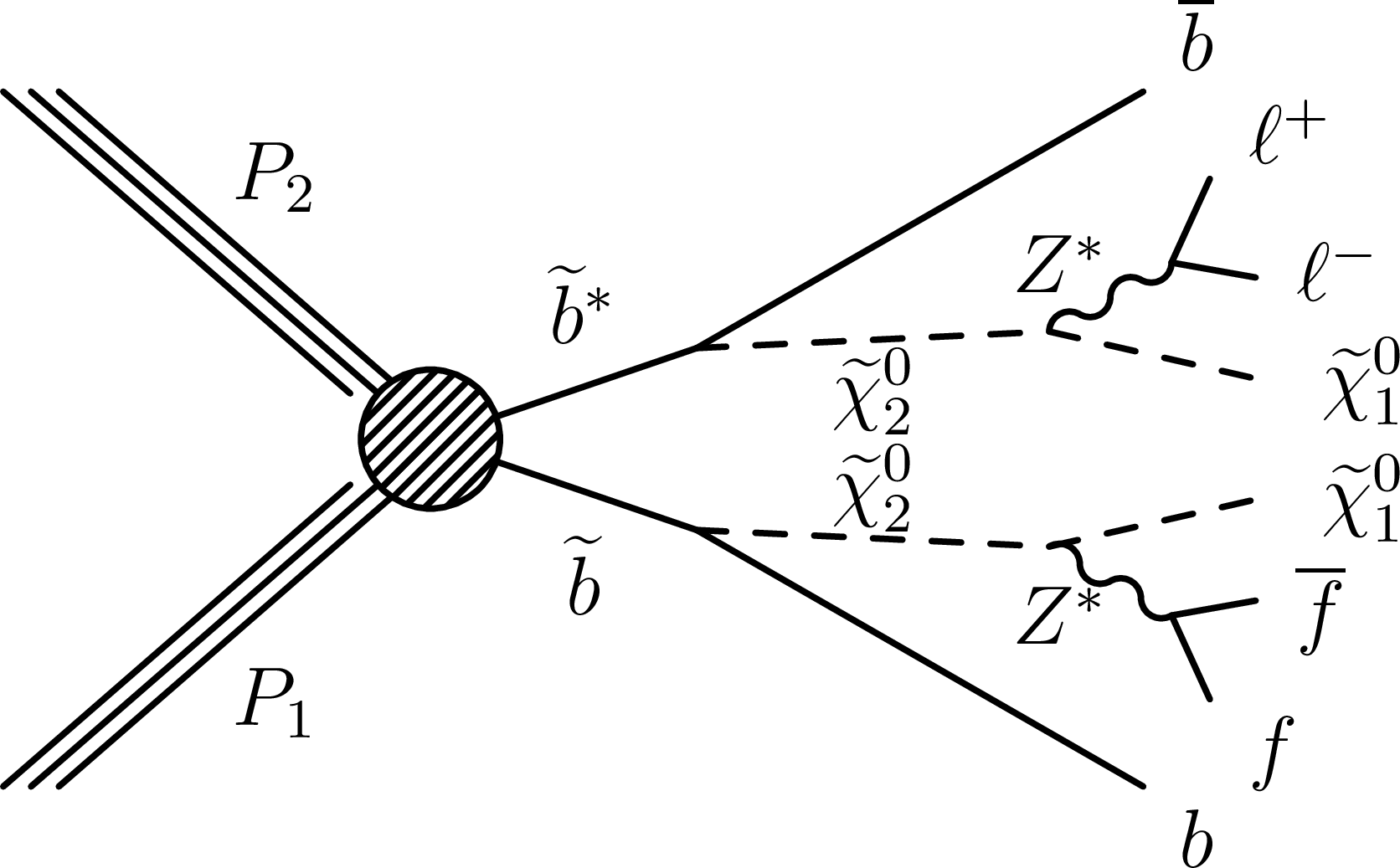
Figure 1-a:
Event diagrams for the (a) ``fixed-edge'', and (b) ``slepton-edge'' scenarios, with $ \mathrm{ \tilde{b} } $ a bottom squark, $ {\tilde{\chi}^{0}_{2}} $ the second lightest neutralino, $ {\tilde{\chi}^{0}_{1}} $ a massive neutralino LSP, and $ \tilde{ \ell } $ an electron- or muon-type slepton. For the slepton-edge scenario, the Z boson can be either on- or off-shell, while for the fixed-edge scenario it is off-shell. |

png pdf |
Figure 1-b:
Event diagrams for the (a) ``fixed-edge'', and (b) ``slepton-edge'' scenarios, with $ \mathrm{ \tilde{b} } $ a bottom squark, $ {\tilde{\chi}^{0}_{2}} $ the second lightest neutralino, $ {\tilde{\chi}^{0}_{1}} $ a massive neutralino LSP, and $ \tilde{ \ell } $ an electron- or muon-type slepton. For the slepton-edge scenario, the Z boson can be either on- or off-shell, while for the fixed-edge scenario it is off-shell. |
png pdf |
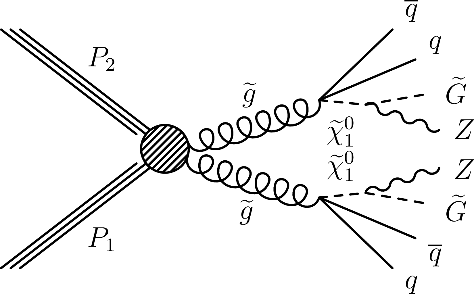
Figure 2:
Event diagram for the ``GMSB'' scenario, with $ \mathrm{ \tilde{g} }$ a gluino, $ {\tilde{\chi}^{0}_{1}} $ the lightest neutralino, and $ \mathrm{ \tilde {G } } $ a massless gravitino LSP. |
png pdf |
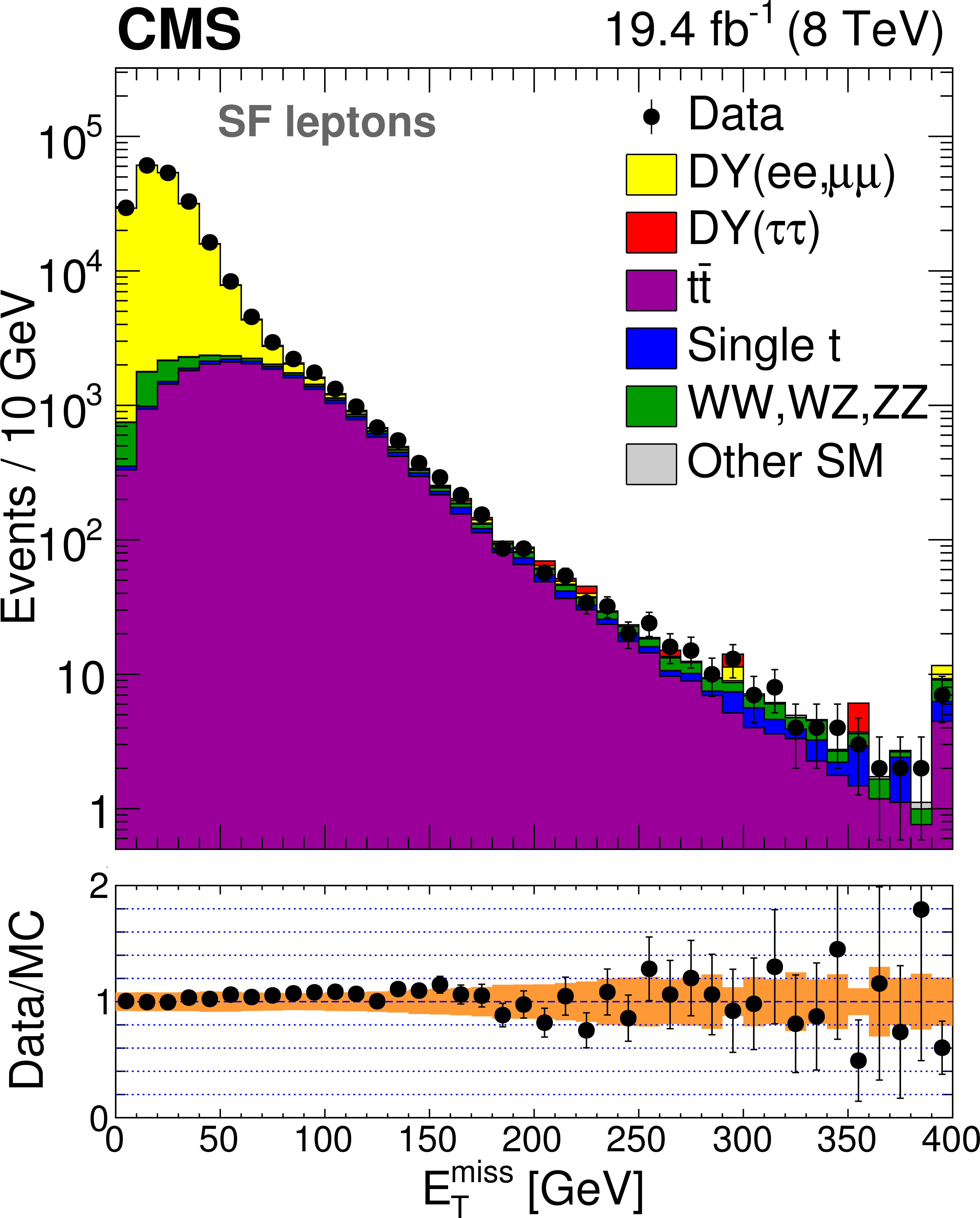
Figure 3-a:
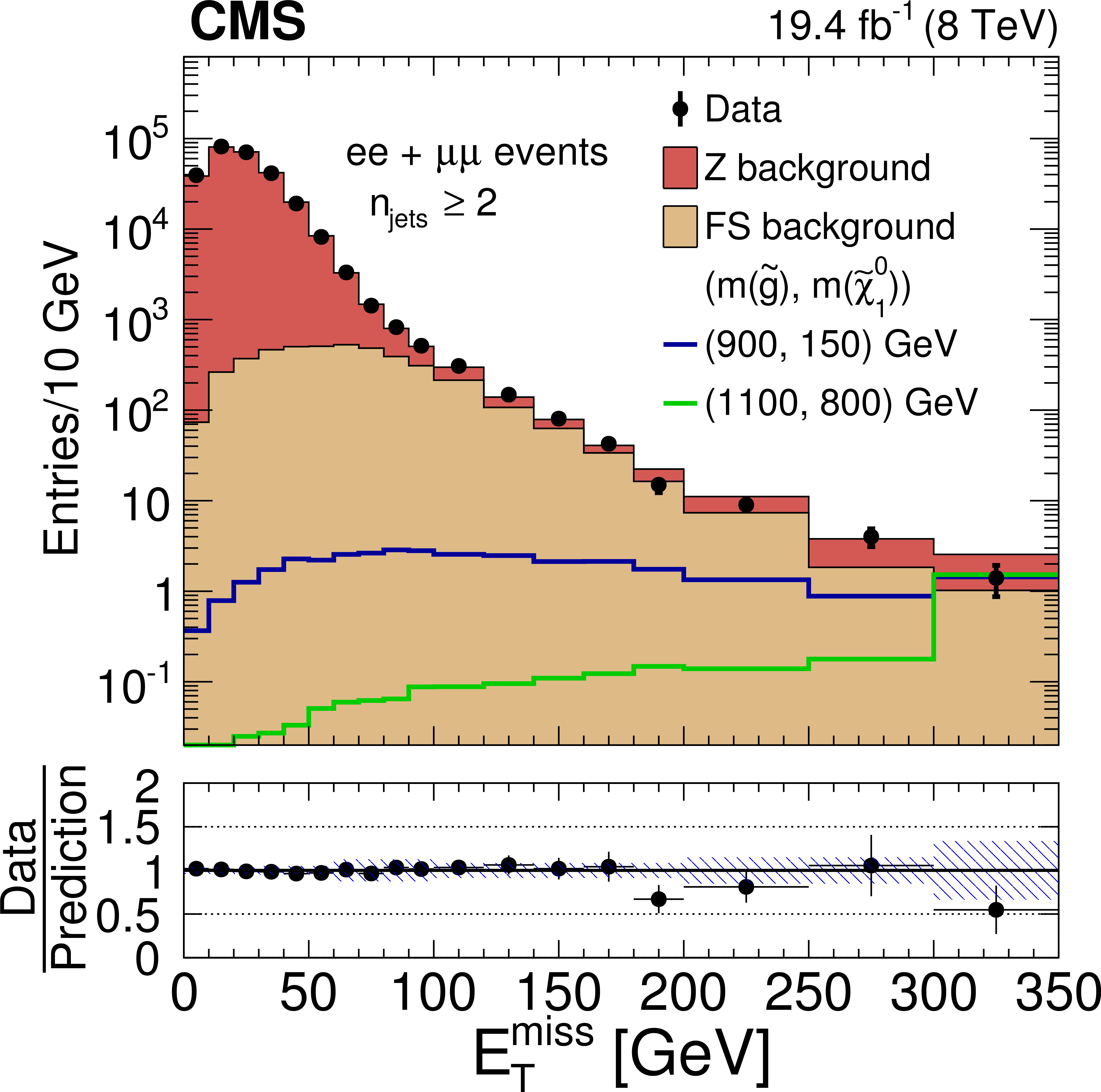
The $ {E_{\mathrm {T}}^{\text {miss}}} $ distributions of events in the SF (a) and OF (b) samples for $m_{\ell \ell }>$ 20 GeV and $N_\text {jets} \geq 2$ in comparison with predictions for the SM background from the MC generators described in Section Event Selection. In the ratio panel below each plot, the error bars on the black points show the statistical uncertainties of the data and MC samples, while the shaded band indicates the MC statistical and systematic uncertainties added in quadrature. The rightmost bins contain the overflow. |
png pdf |
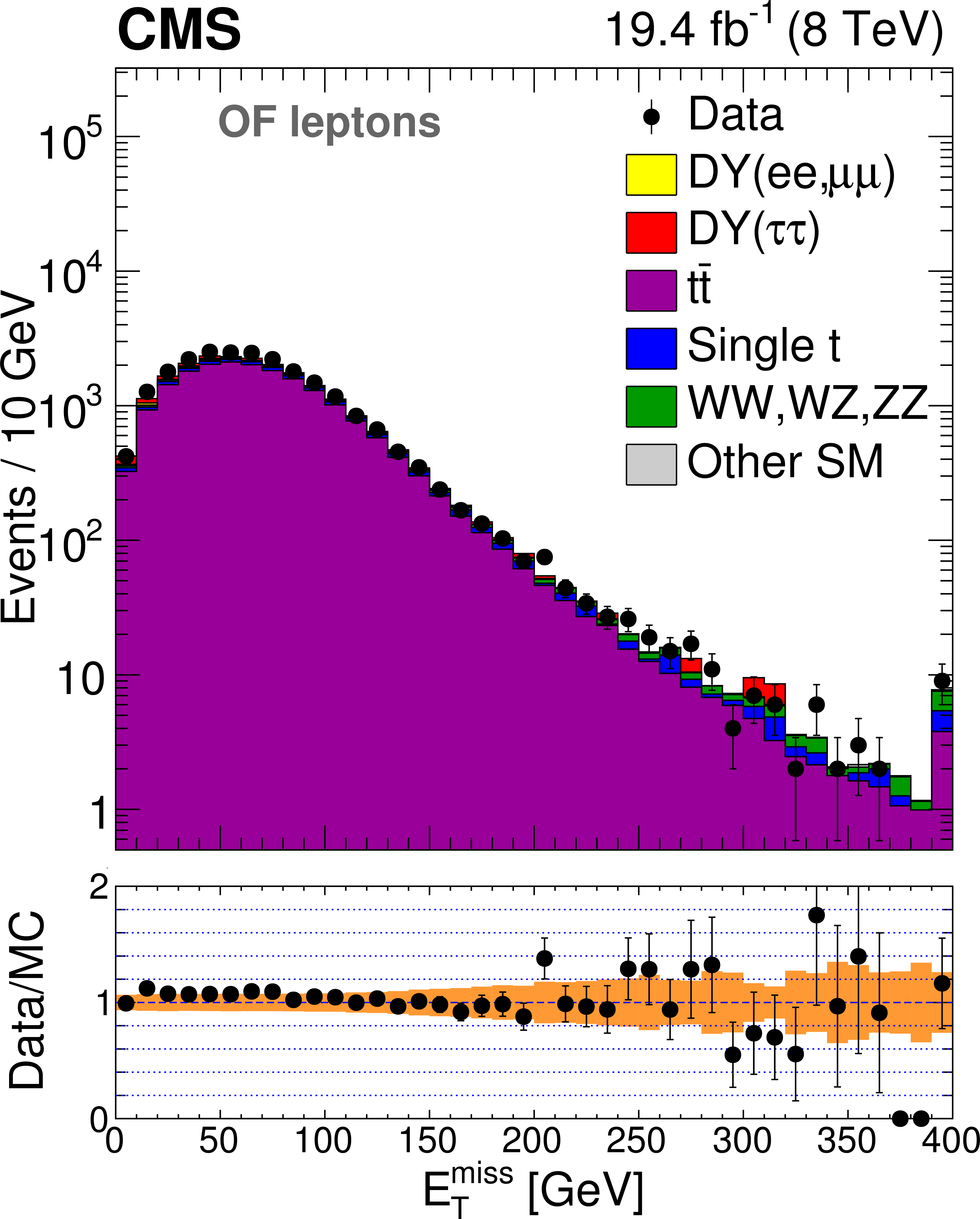
Figure 3-b:
The $ {E_{\mathrm {T}}^{\text {miss}}} $ distributions of events in the SF (a) and OF (b) samples for $m_{\ell \ell }>$ 20 GeV and $N_\text {jets} \geq 2$ in comparison with predictions for the SM background from the MC generators described in Section Event Selection. In the ratio panel below each plot, the error bars on the black points show the statistical uncertainties of the data and MC samples, while the shaded band indicates the MC statistical and systematic uncertainties added in quadrature. The rightmost bins contain the overflow. |
png pdf |
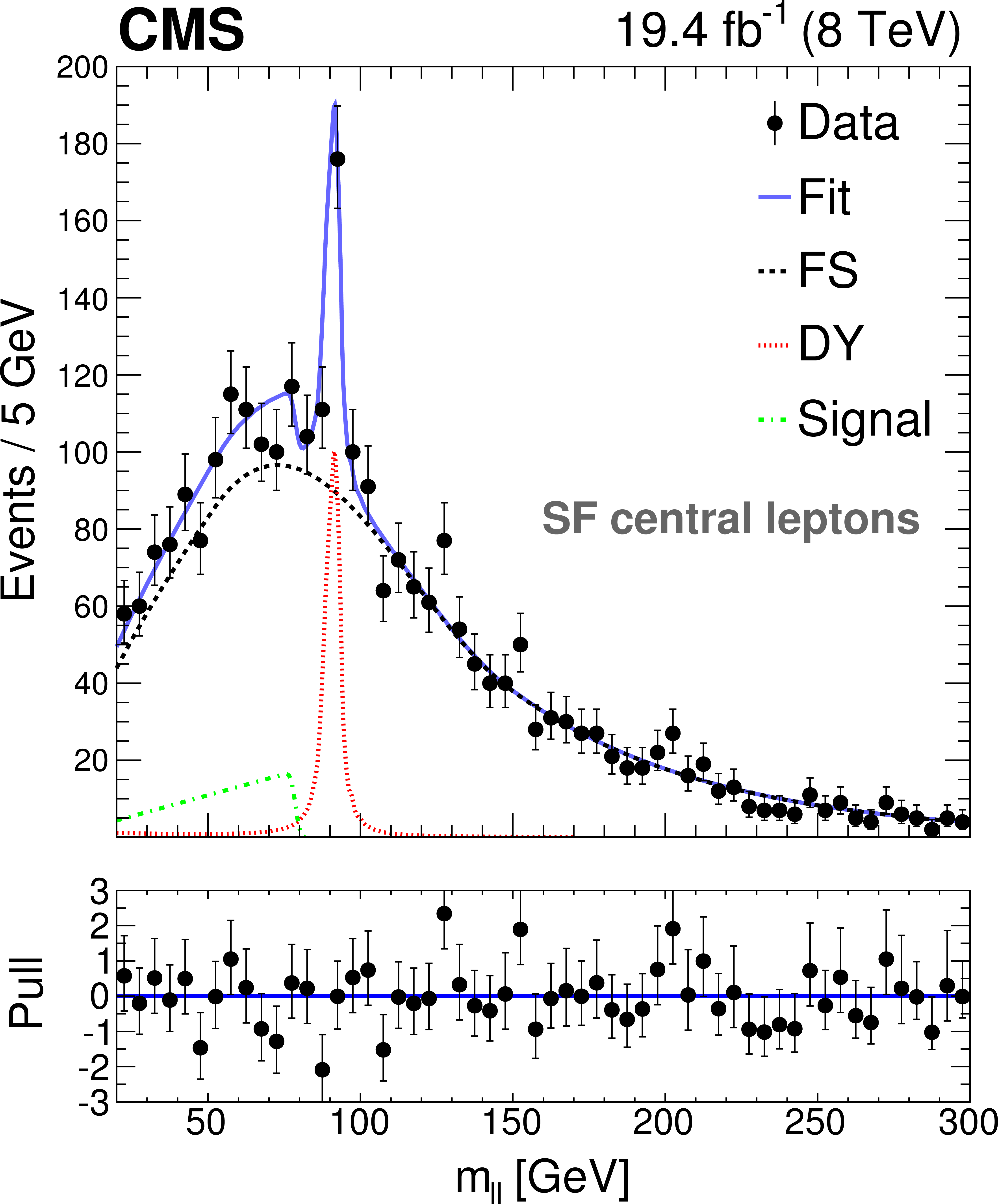
Figure 4-a:
Fit results for the signal-plus-background hypothesis in comparison with the measured dilepton mass distributions, in the central (a, b) and forward (c, d) regions, projected on the same-flavor (a, c) and opposite-flavor (b, d) event samples. The combined fit shape is shown as a blue, solid line. The individual fit components are indicated by dashed lines. The flavor-symmetric (FS) background is displayed with a black dashed line. The Drell--Yan (DY) background is displayed with a red dashed line. The extracted signal component is displayed with a green dashed line. The lower plots show the pull distributions, defined as $(N_\text {data} - N_\text {fit})/\sigma _\text {data}$. |
png pdf |
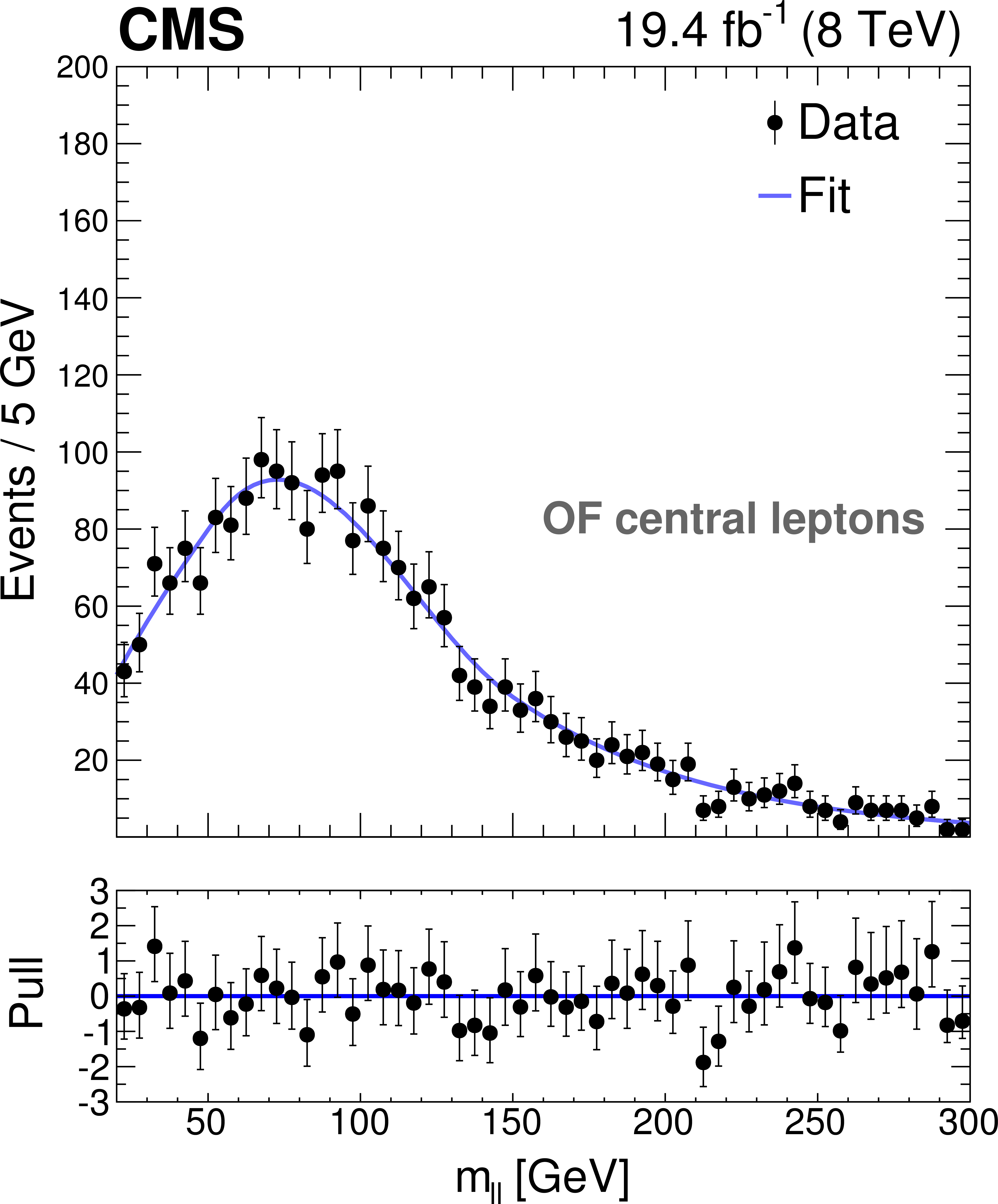
Figure 4-b:
Fit results for the signal-plus-background hypothesis in comparison with the measured dilepton mass distributions, in the central (a, b) and forward (c, d) regions, projected on the same-flavor (a, c) and opposite-flavor (b, d) event samples. The combined fit shape is shown as a blue, solid line. The individual fit components are indicated by dashed lines. The flavor-symmetric (FS) background is displayed with a black dashed line. The Drell--Yan (DY) background is displayed with a red dashed line. The extracted signal component is displayed with a green dashed line. The lower plots show the pull distributions, defined as $(N_\text {data} - N_\text {fit})/\sigma _\text {data}$. |
png pdf |
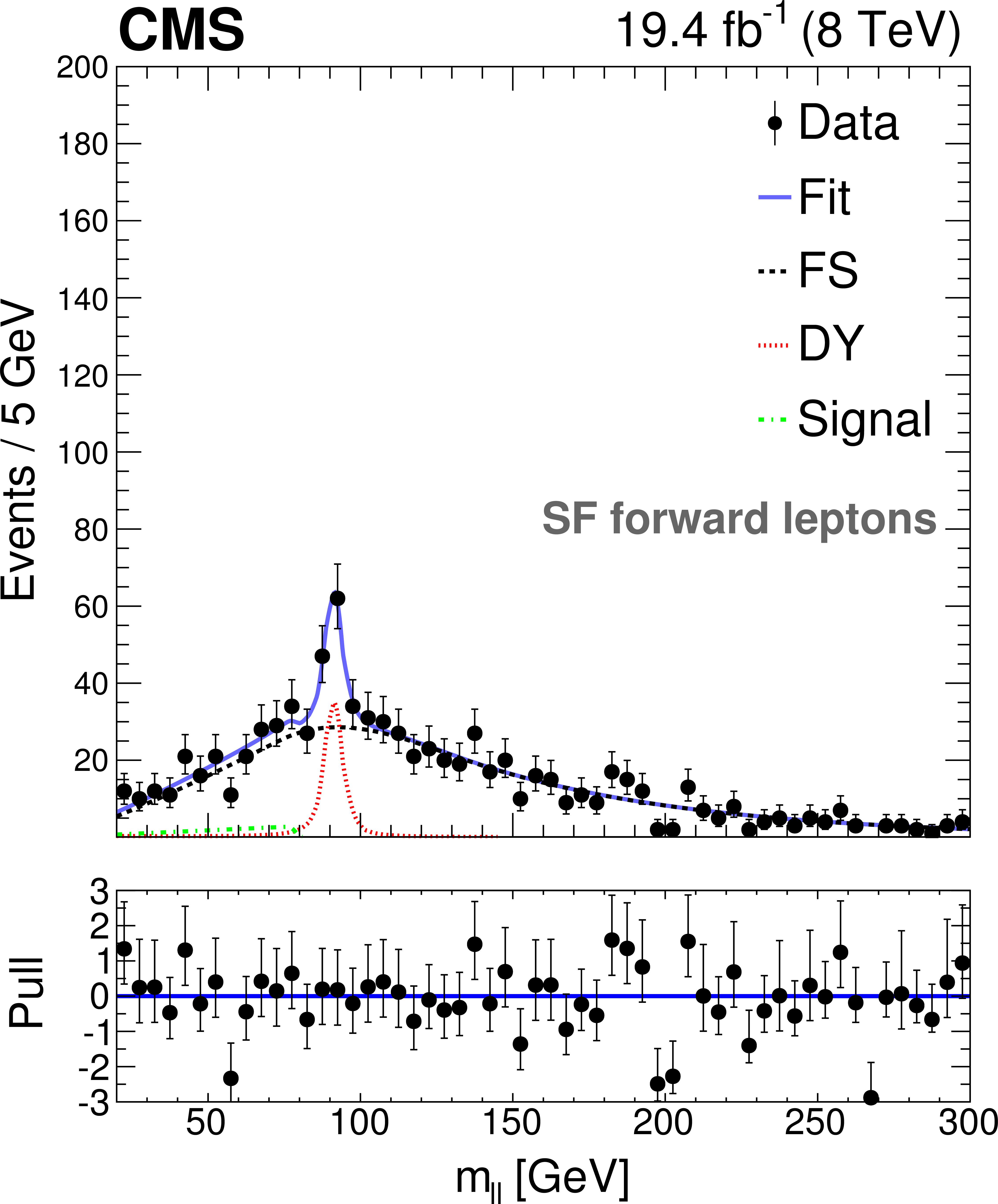
Figure 4-c:
Fit results for the signal-plus-background hypothesis in comparison with the measured dilepton mass distributions, in the central (a, b) and forward (c, d) regions, projected on the same-flavor (a, c) and opposite-flavor (b, d) event samples. The combined fit shape is shown as a blue, solid line. The individual fit components are indicated by dashed lines. The flavor-symmetric (FS) background is displayed with a black dashed line. The Drell--Yan (DY) background is displayed with a red dashed line. The extracted signal component is displayed with a green dashed line. The lower plots show the pull distributions, defined as $(N_\text {data} - N_\text {fit})/\sigma _\text {data}$. |
png pdf |
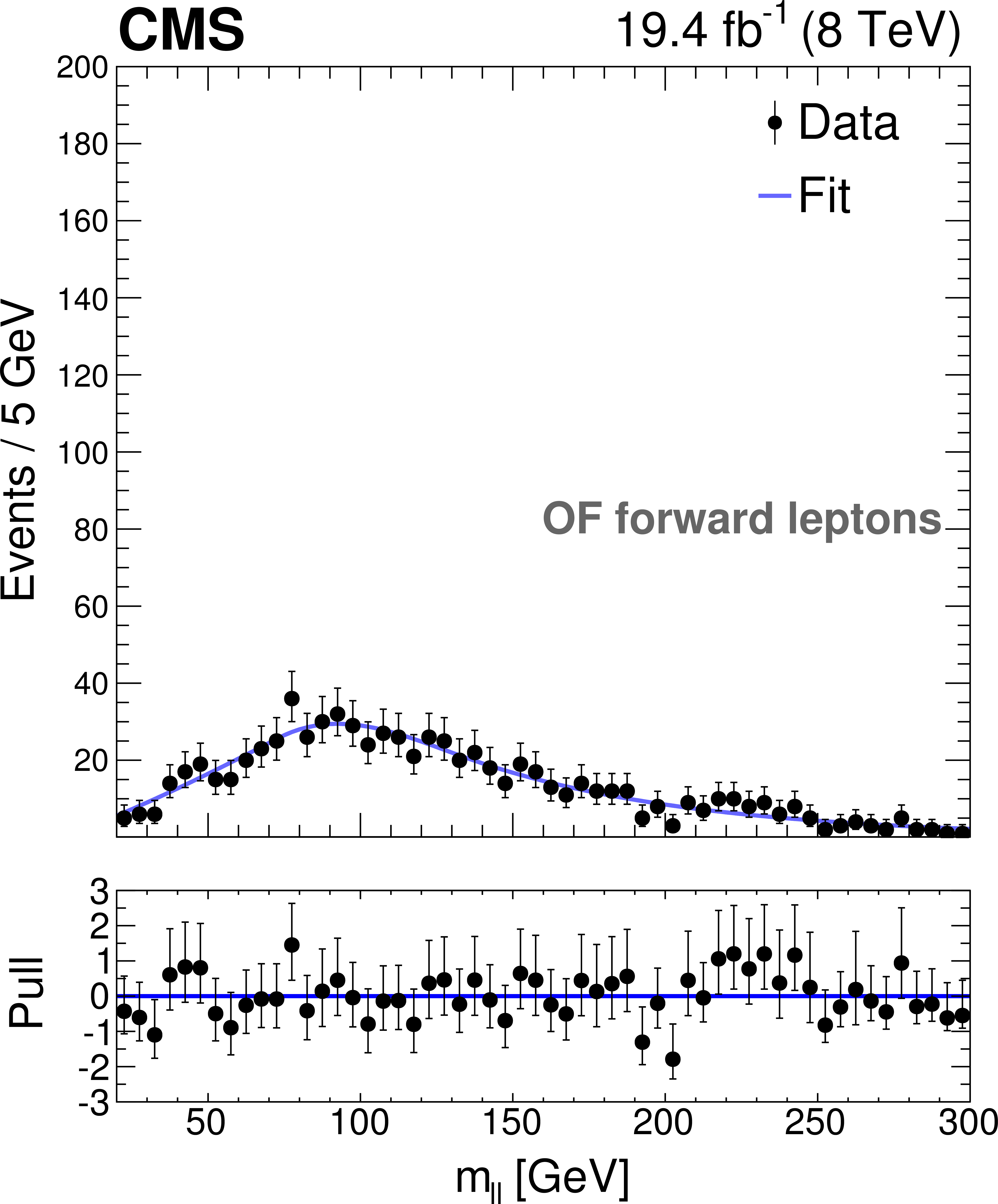
Figure 4-d:
Fit results for the signal-plus-background hypothesis in comparison with the measured dilepton mass distributions, in the central (a, b) and forward (c, d) regions, projected on the same-flavor (a, c) and opposite-flavor (b, d) event samples. The combined fit shape is shown as a blue, solid line. The individual fit components are indicated by dashed lines. The flavor-symmetric (FS) background is displayed with a black dashed line. The Drell--Yan (DY) background is displayed with a red dashed line. The extracted signal component is displayed with a green dashed line. The lower plots show the pull distributions, defined as $(N_\text {data} - N_\text {fit})/\sigma _\text {data}$. |
png pdf |
Figure 5-a:
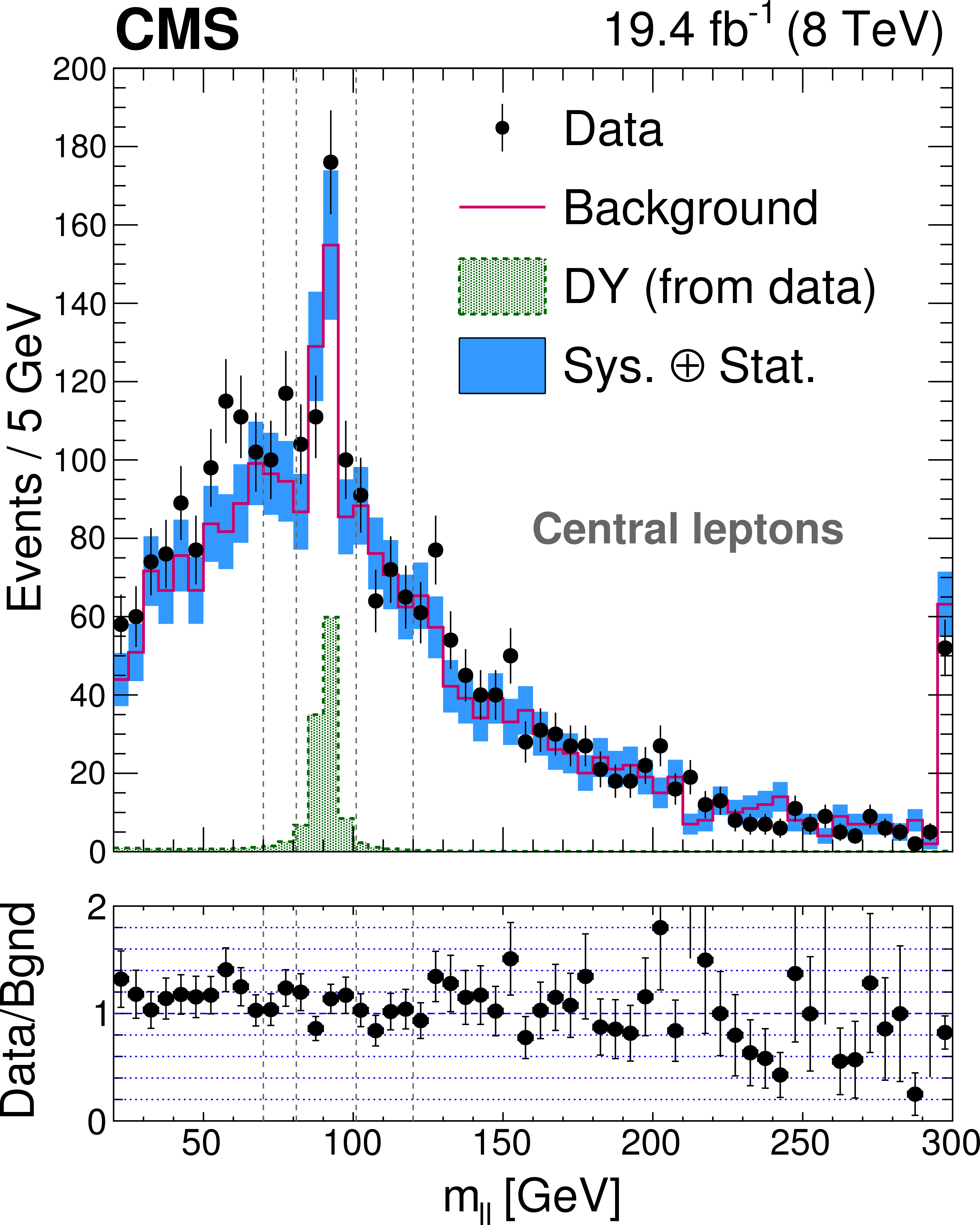
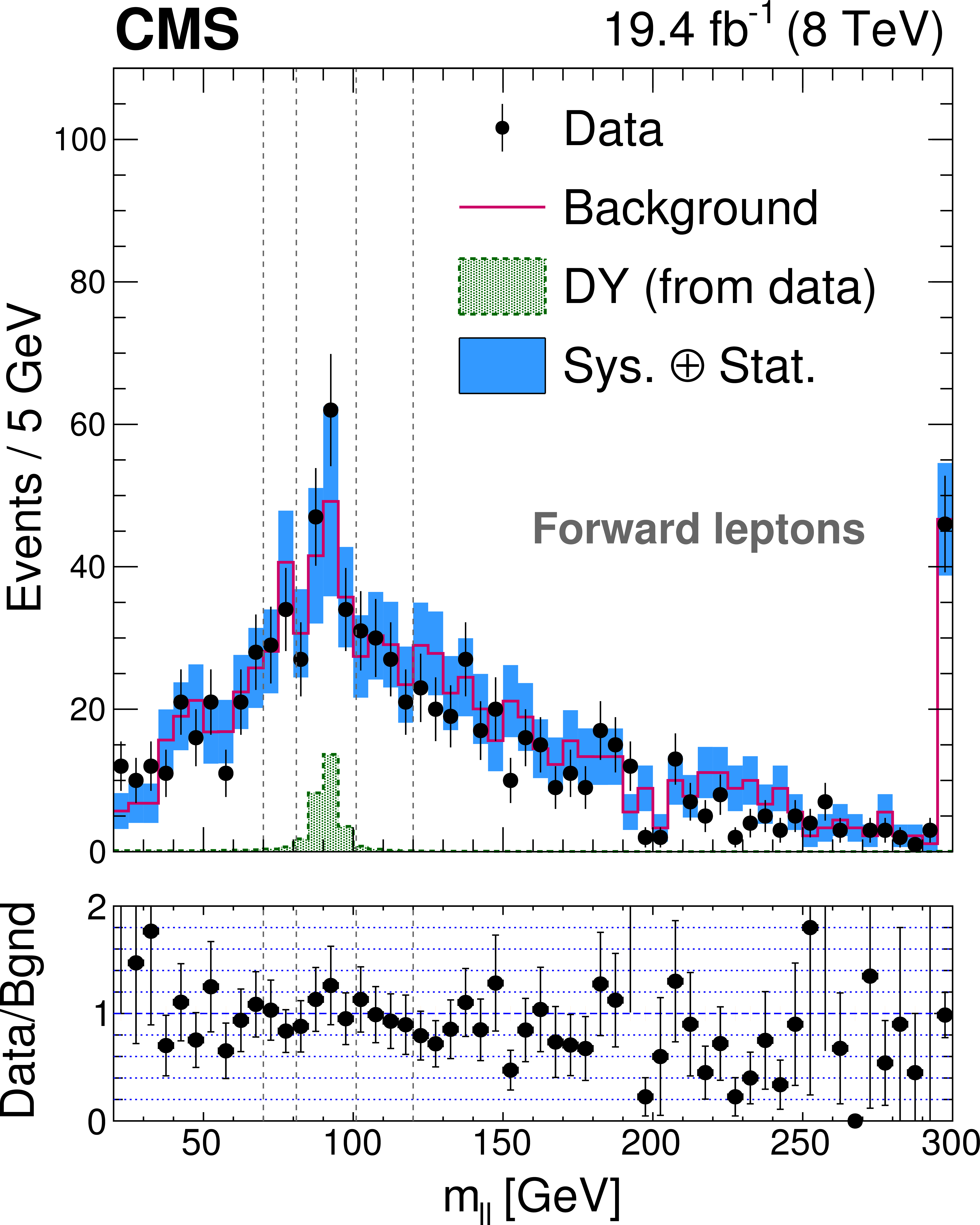
Comparison between the observed and estimated SM background dilepton mass distributions in the (a) central and (b) forward regions, where the SM backgrounds are evaluated from control samples (see text) rather than from a fit. The rightmost bins contain the overflow. The vertical dashed lines denote the boundaries of the low-mass, on-Z, and high-mass regions. The lower plots show the ratio of the data to the predicted background. The error bars for both the main and lower plots include both statistical and systematic uncertainties. |
png pdf |
Figure 5-b:
Comparison between the observed and estimated SM background dilepton mass distributions in the (a) central and (b) forward regions, where the SM backgrounds are evaluated from control samples (see text) rather than from a fit. The rightmost bins contain the overflow. The vertical dashed lines denote the boundaries of the low-mass, on-Z, and high-mass regions. The lower plots show the ratio of the data to the predicted background. The error bars for both the main and lower plots include both statistical and systematic uncertainties. |

png pdf |
Figure 6-a:
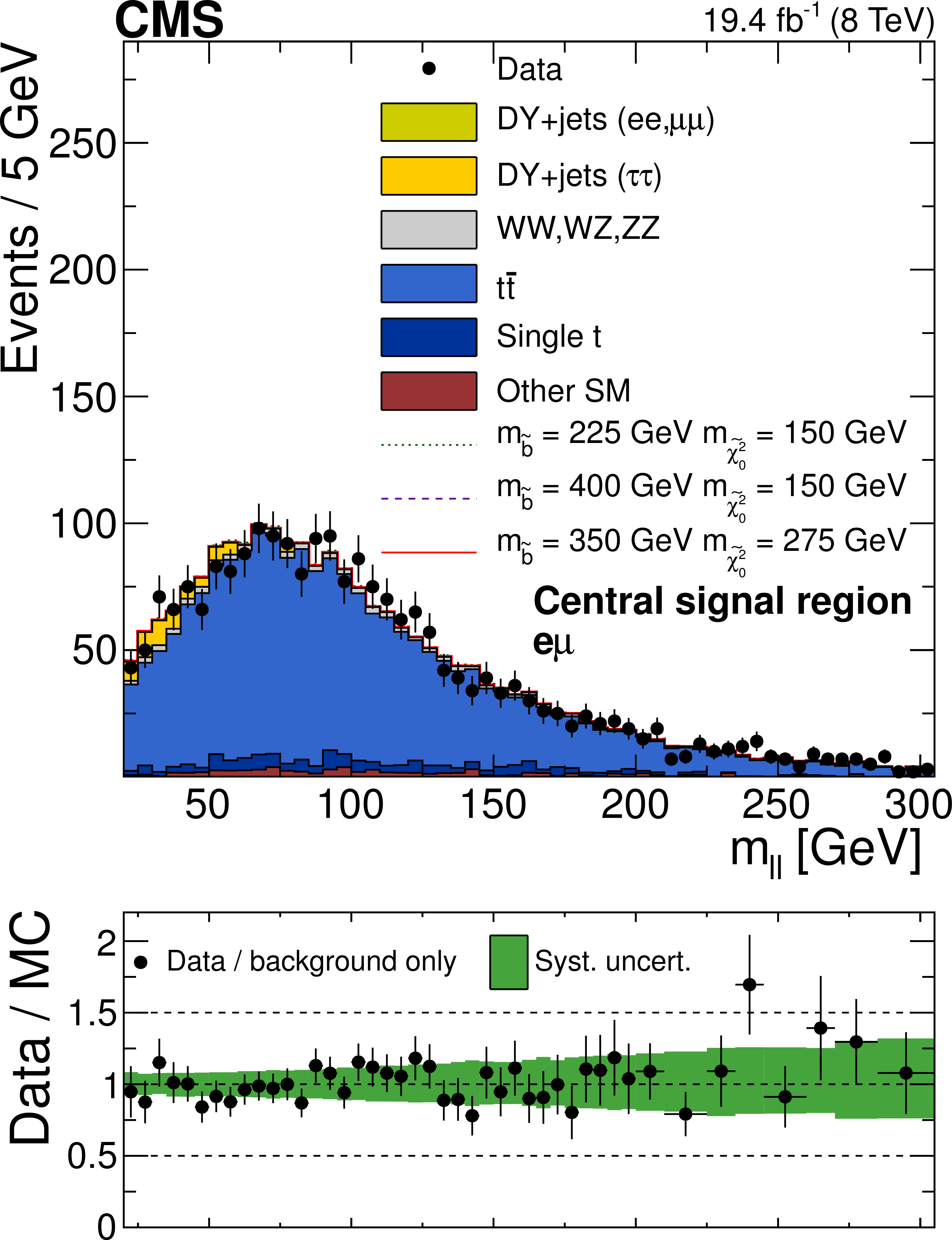
Data compared with SM simulation for the SF (a) and OF (b) event samples in the central region. Example signal scenarios based on the pair production of bottom squarks are shown (see text). In the ratio panel below each plot, the error bars on the points show the statistical uncertainties of the data and MC samples, while the shaded band indicates the MC systematic uncertainty. |
png pdf |
Figure 6-b:
Data compared with SM simulation for the SF (a) and OF (b) event samples in the central region. Example signal scenarios based on the pair production of bottom squarks are shown (see text). In the ratio panel below each plot, the error bars on the points show the statistical uncertainties of the data and MC samples, while the shaded band indicates the MC systematic uncertainty. |
png pdf |
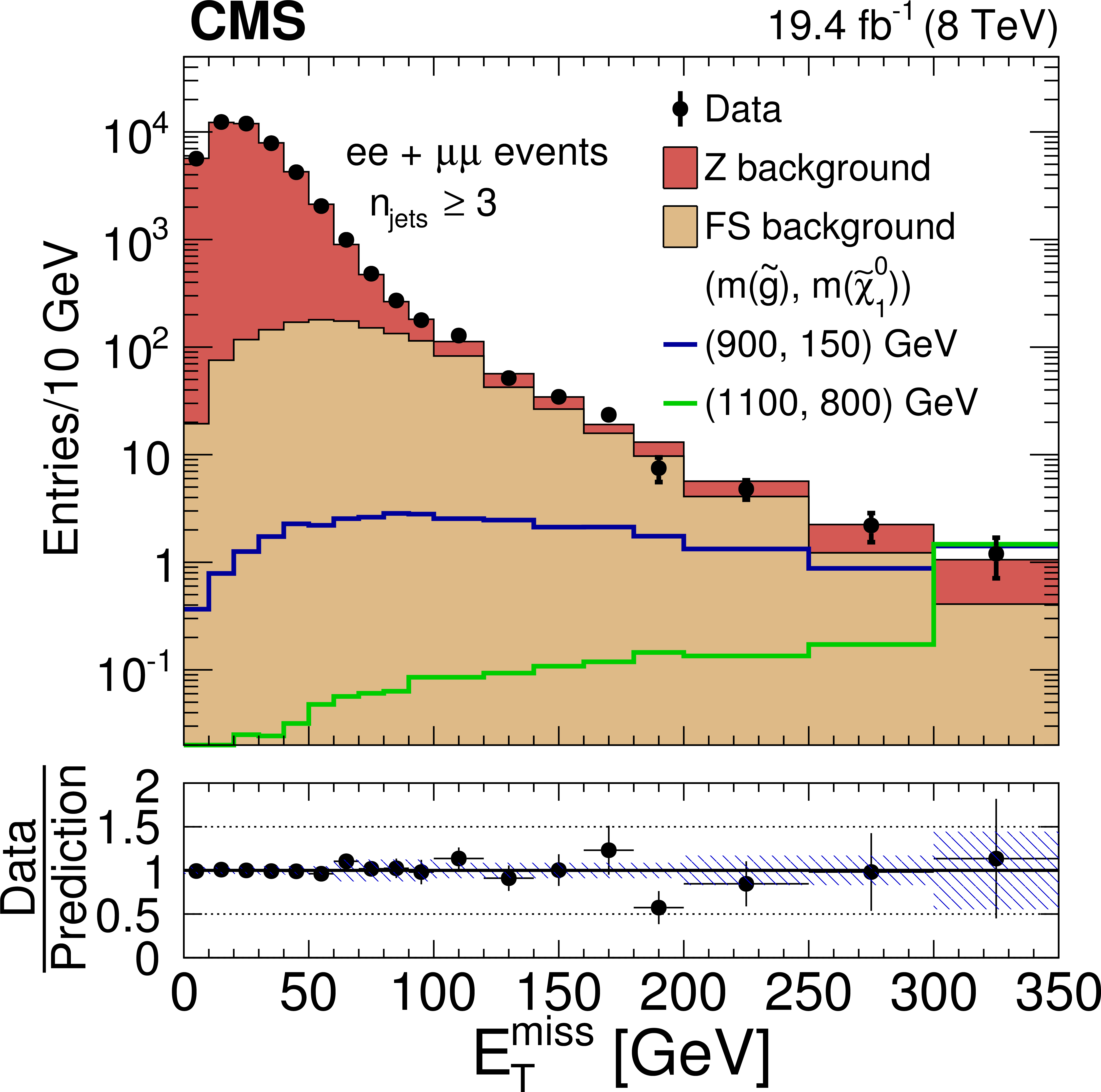
Figure 7-a:
The $ {E_{\mathrm {T}}^{\text {miss}}} $ distributions for the on- Z signal regions with (q) $\geq $2jets and (b) $\geq $3jets. The uncertainty band shown for the ratio includes both statistical and systematic uncertainties. Additionally, $ {E_{\mathrm {T}}^{\text {miss}}} $ distributions are drawn for two choices of masses in the GMSB scenario. The rightmost bins contain the overflow. |
png pdf |
Figure 7-b:
The $ {E_{\mathrm {T}}^{\text {miss}}} $ distributions for the on- Z signal regions with (q) $\geq $2jets and (b) $\geq $3jets. The uncertainty band shown for the ratio includes both statistical and systematic uncertainties. Additionally, $ {E_{\mathrm {T}}^{\text {miss}}} $ distributions are drawn for two choices of masses in the GMSB scenario. The rightmost bins contain the overflow. |
png pdf |
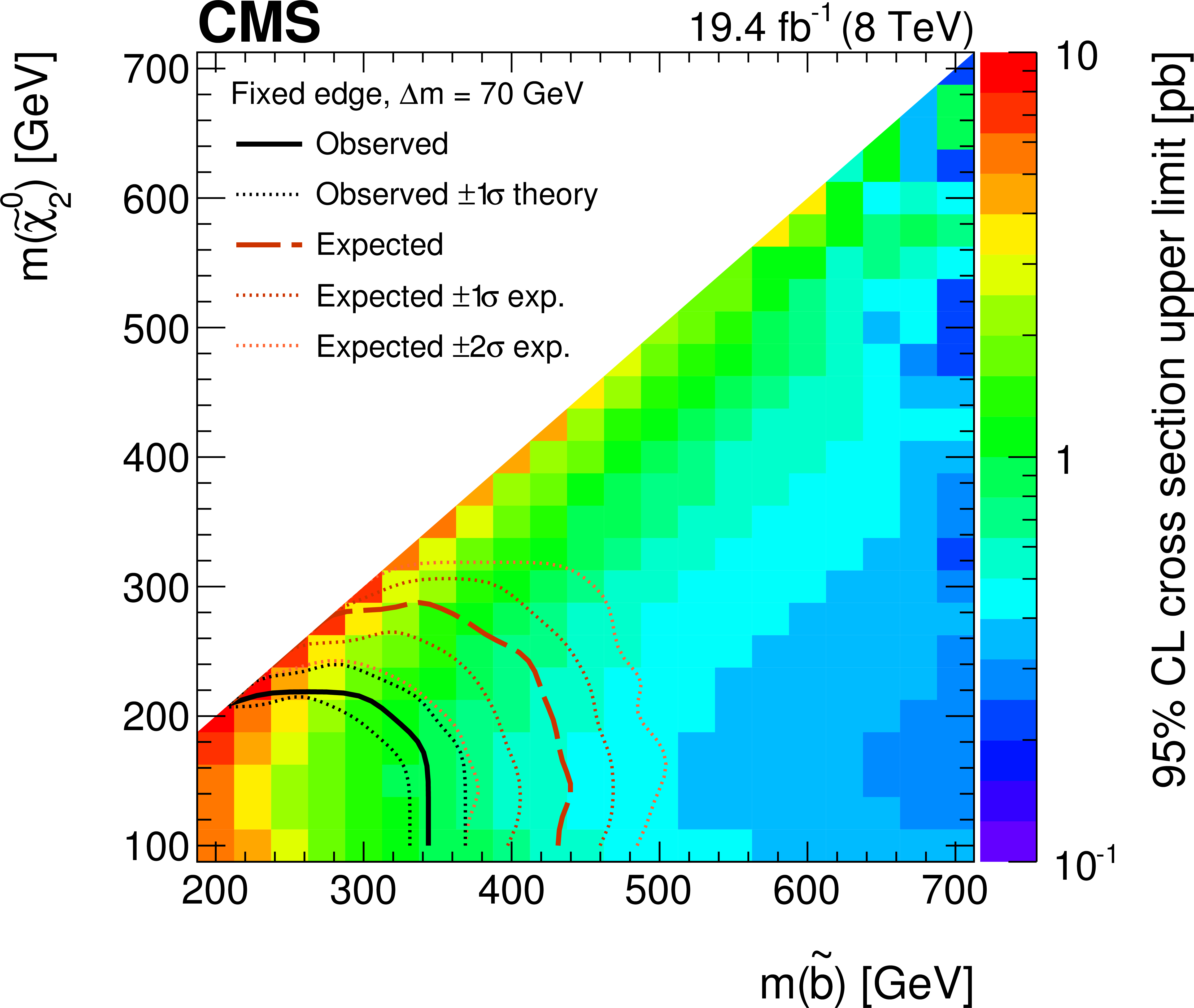
Figure 8-a:
Exclusion limits at 95% CL for the fixed- (a) and slepton-edge (b) scenarios in the $m_{ \mathrm{ \tilde{b} } }$-$m_{ {\tilde{\chi}^{0}_{2}} }$ plane. The color indicates the excluded cross section for each considered point in parameter space. The intersections of the theoretical cross section with the expected and observed limits are indicated by the solid and hatched lines. The 1 standard deviation ($\sigma $) experimental and theoretical uncertainty contours are shown as dotted lines. |
png pdf |
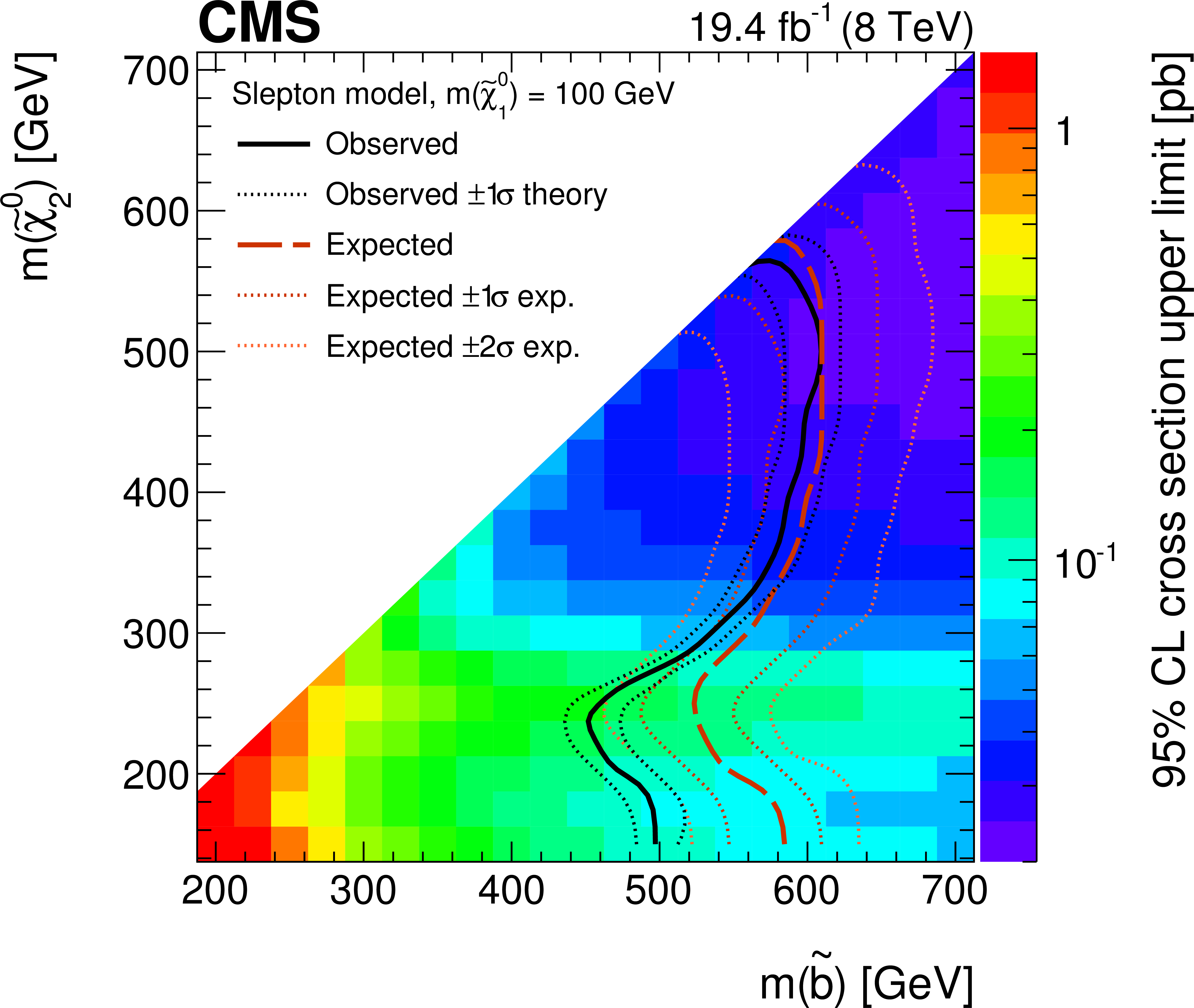
Figure 8-b:
Exclusion limits at 95% CL for the fixed- (a) and slepton-edge (b) scenarios in the $m_{ \mathrm{ \tilde{b} } }$-$m_{ {\tilde{\chi}^{0}_{2}} }$ plane. The color indicates the excluded cross section for each considered point in parameter space. The intersections of the theoretical cross section with the expected and observed limits are indicated by the solid and hatched lines. The 1 standard deviation ($\sigma $) experimental and theoretical uncertainty contours are shown as dotted lines. |
png pdf |
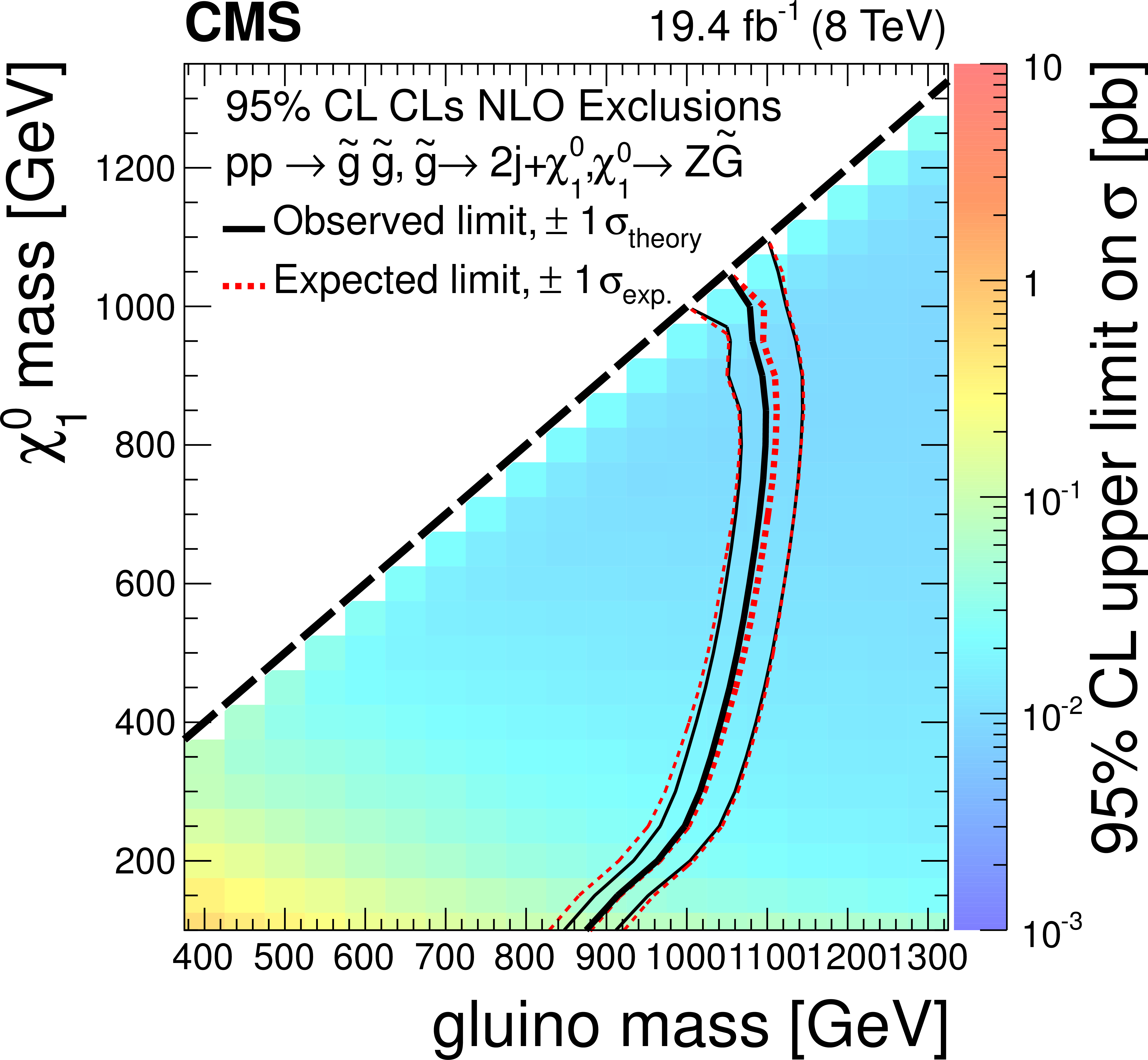
Figure 9:
Exclusion limits at 95% CL for the GMSB scenario in the $m_{ \mathrm{ \tilde{g} }}$-$m_{ {\tilde{\chi}^{0}_{1}} }$ plane. The color indicates the excluded cross section for each considered point in parameter space. The intersections of the theoretical cross section with the expected and observed limits are indicated by the solid and hatched lines. The 1 standard deviation ($\sigma $) experimental and theoretical uncertainty contours are shown as dotted lines. |
|
|
Compact Muon Solenoid LHC, CERN |
|

|

|

|

|

|