

Compact Muon Solenoid
LHC, CERN
| CMS-SUS-14-015 ; CERN-PH-EP-2016-004 | ||
| Search for direct pair production of scalar top quarks in the single- and dilepton channels in proton-proton collisions at $ \sqrt{s} = $ 8 TeV | ||
| CMS Collaboration | ||
| 10 February 2016 | ||
| JHEP 07 (2016) 027 [Erratum] | ||
| Abstract: Results are reported from a search for the top squark $ \tilde{ \mathrm{t} }_1 $, the lighter of the two supersymmetric partners of the top quark. The data sample corresponds to 19.7 fb$^{-1}$ of proton-proton collisions at $ \sqrt{s} = $ 8 TeV collected with the CMS detector at the LHC. The search targets $ \tilde{ \mathrm{t} }_1 \to \mathrm{b } \tilde{ \chi }^{\pm}_1$ and $ \tilde{ \mathrm{t} }_1 \to \mathrm{t }^{(*)} \tilde{\chi}^0_1$ decay modes, where $\tilde{ \chi }^{\pm}_1$ and $\tilde{\chi}^0_1$ are the lightest chargino and neutralino, respectively. The reconstructed final state consists of jets, b jets, missing transverse energy, and either one or two leptons. Leading backgrounds are determined from data. No significant excess in data is observed above the expectation from standard model processes. The results exclude a region of the two-dimensional plane of possible $ \tilde{ \mathrm{t} }_1 $ and ${\tilde{\chi}^0_1} $ masses. The highest excluded $ \tilde{ \mathrm{t} }_1 $ and ${\tilde{\chi}^0_1} $ masses are about 700 GeV and 250 GeV, respectively. | ||
| Links: e-print arXiv:1602.03169 [hep-ex] (PDF) ; CDS record ; inSPIRE record ; CADI line (restricted) ; | ||
| Figures | |
png pdf |
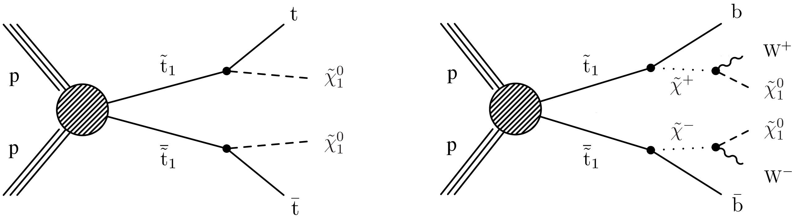
Figure 1:
Top squark direct pair production at the LHC. Left: tt decay mode. Right: bbWW decay mode. |

png pdf |
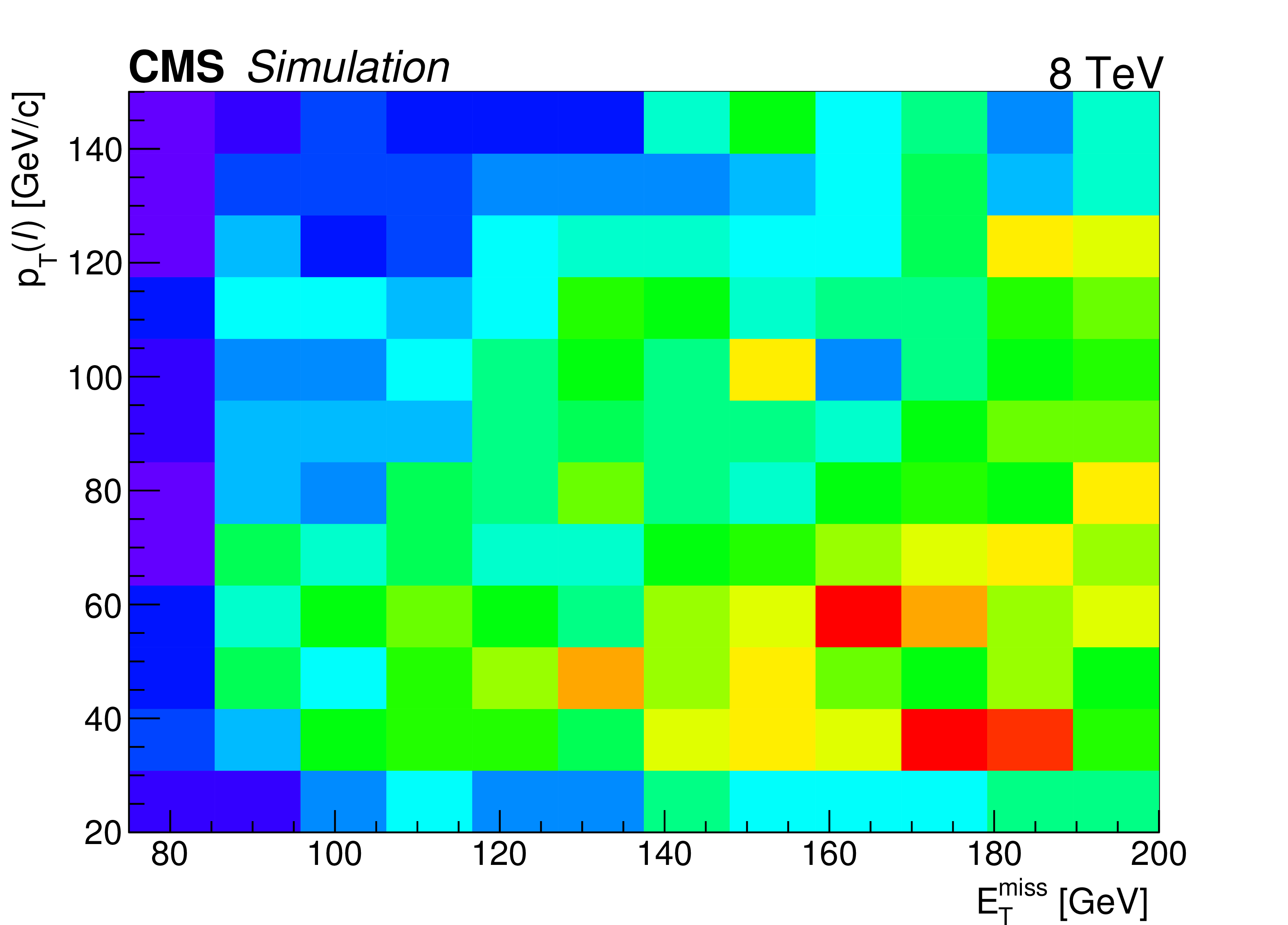
Figure 2-a:
Distribution of the transverse momentum of the lepton versus the missing transverse energy at the preselection, for the simulated ${\mathrm {t}\overline {\mathrm {t}}}$ background (a) and for the bbWW decay mode ($x=$ 0.50) of the signal with $ m( \tilde{ \mathrm{t} }_{1} )-m( { {\tilde{\chi}^{0}_{1}} } ) \geq $ 625 GeV (b). |
png pdf |
Figure 2-b:
Distribution of the transverse momentum of the lepton versus the missing transverse energy at the preselection, for the simulated ${\mathrm {t}\overline {\mathrm {t}}}$ background (a) and for the bbWW decay mode ($x=$ 0.50) of the signal with $ m( \tilde{ \mathrm{t} }_{1} )-m( { {\tilde{\chi}^{0}_{1}} } ) \geq $ 625 GeV (b). |
png |
Figure 2-c:
Distribution of the transverse momentum of the lepton versus the missing transverse energy at the preselection, for the simulated ${\mathrm {t}\overline {\mathrm {t}}}$ background (a) and for the bbWW decay mode ($x=$ 0.50) of the signal with $ m( \tilde{ \mathrm{t} }_{1} )-m( { {\tilde{\chi}^{0}_{1}} } ) \geq $ 625 GeV (b). |
png pdf |
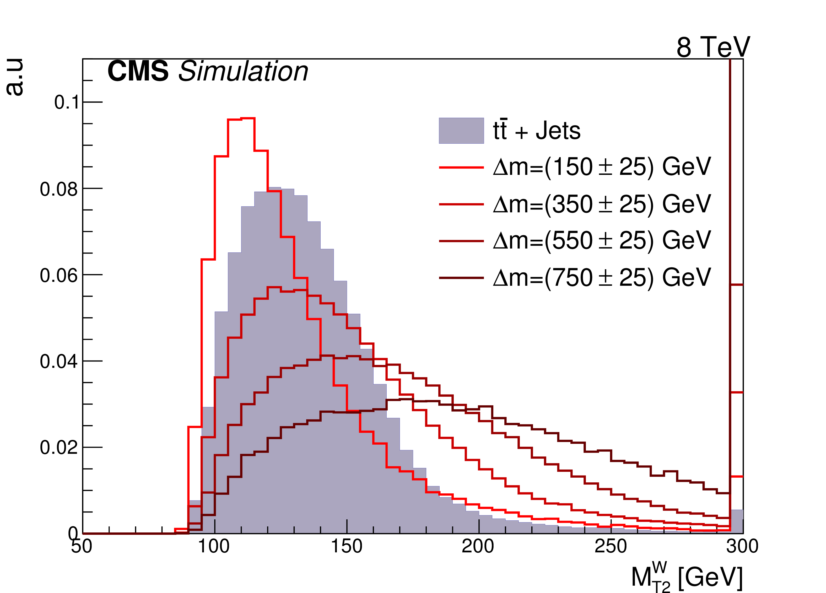
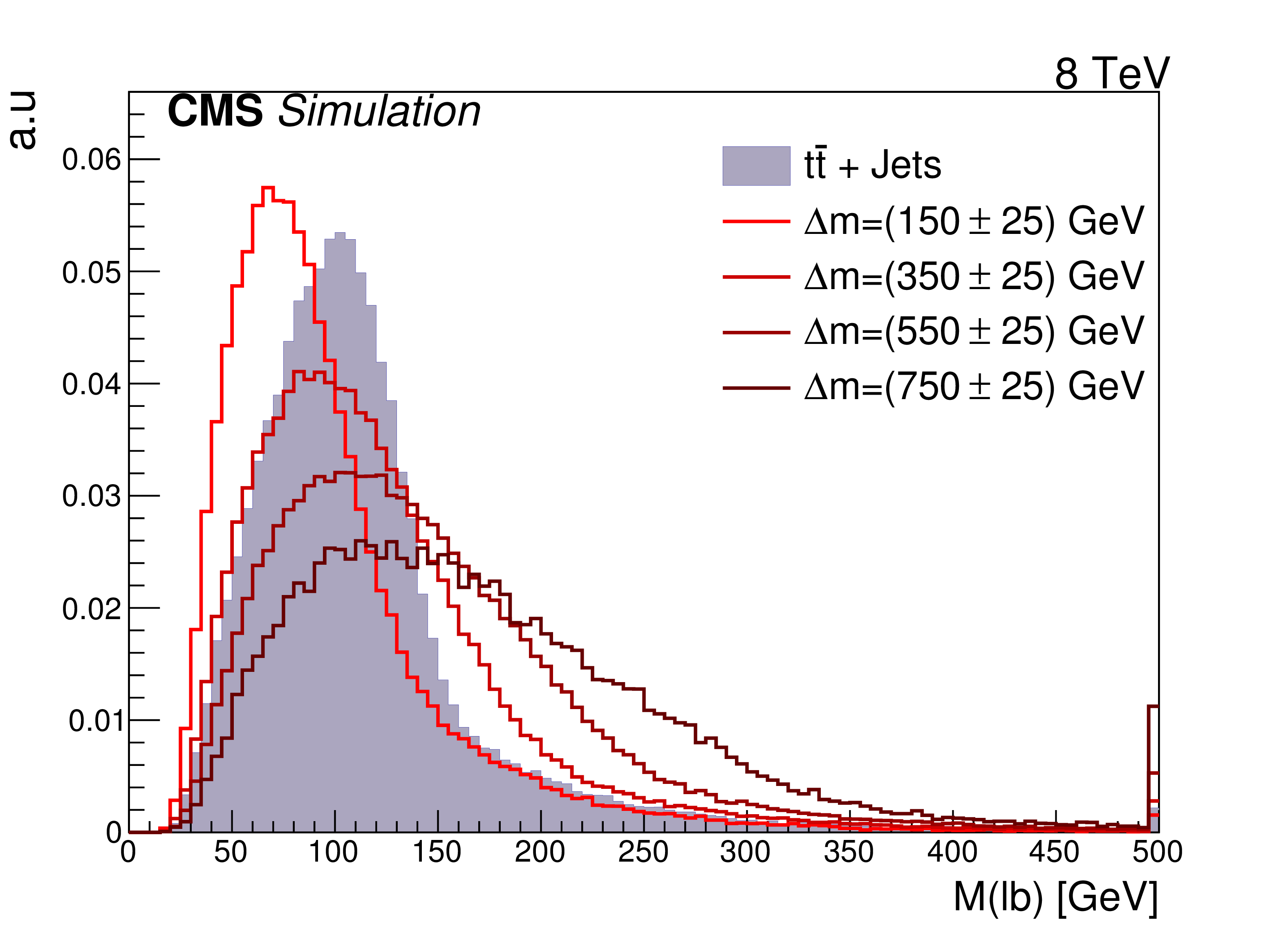
Figure 3-a:
Distribution of some discriminating variables for the bbWW ($x=$ 0.75) decay mode at the preselection level, for the main $ {\mathrm {t}\overline {\mathrm {t}}} $ background and benchmark signal mass points grouped in bands of constant width $ {\Delta m} =$ (150 $\pm$ 25 ), (350 $\pm$ 25 ), (550 $\pm$ 25 ), and (750 $\pm$ 25 ) GeV. Distributions are normalized to the same area. From (a) to (d): ${M_{{\mathrm T}2}^{ {\mathrm {W}}}} $, ${M(\text {3 jet})} $, ${M(\ell {\mathrm {b}})} and {N(\text {jets})} $. |

png pdf |
Figure 3-b:
Distribution of some discriminating variables for the bbWW ($x=$ 0.75) decay mode at the preselection level, for the main $ {\mathrm {t}\overline {\mathrm {t}}} $ background and benchmark signal mass points grouped in bands of constant width $ {\Delta m} =$ (150 $\pm$ 25 ), (350 $\pm$ 25 ), (550 $\pm$ 25 ), and (750 $\pm$ 25 ) GeV. Distributions are normalized to the same area. From (a) to (d): ${M_{{\mathrm T}2}^{ {\mathrm {W}}}} $, ${M(\text {3 jet})} $, ${M(\ell {\mathrm {b}})} and {N(\text {jets})} $. |
png pdf |
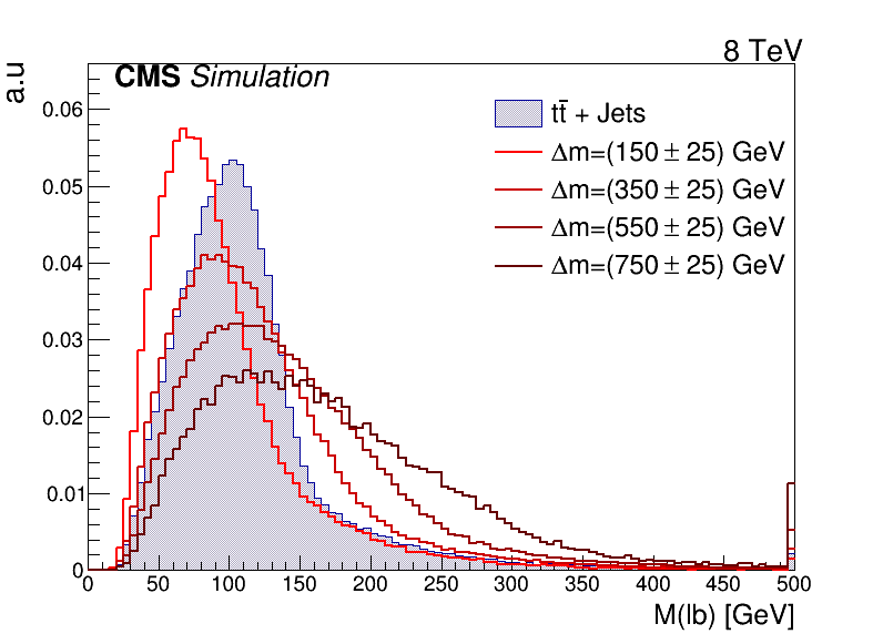
Figure 3-c:
Distribution of some discriminating variables for the bbWW ($x=$ 0.75) decay mode at the preselection level, for the main $ {\mathrm {t}\overline {\mathrm {t}}} $ background and benchmark signal mass points grouped in bands of constant width $ {\Delta m} =$ (150 $\pm$ 25 ), (350 $\pm$ 25 ), (550 $\pm$ 25 ), and (750 $\pm$ 25 ) GeV. Distributions are normalized to the same area. From (a) to (d): ${M_{{\mathrm T}2}^{ {\mathrm {W}}}} $, ${M(\text {3 jet})} $, ${M(\ell {\mathrm {b}})} and {N(\text {jets})} $. |
png pdf |
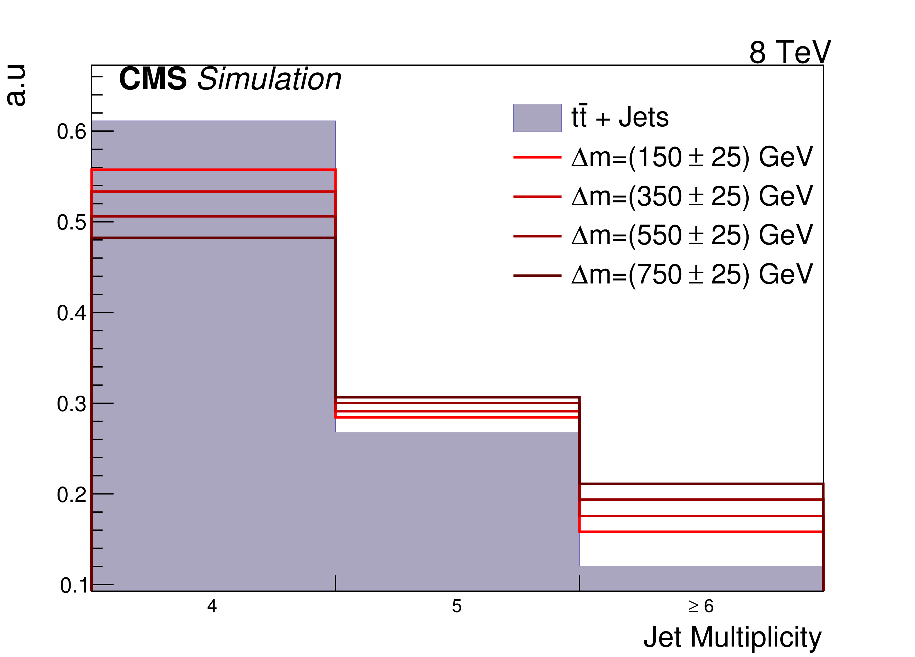
Figure 3-d:
Distribution of some discriminating variables for the bbWW ($x=$ 0.75) decay mode at the preselection level, for the main $ {\mathrm {t}\overline {\mathrm {t}}} $ background and benchmark signal mass points grouped in bands of constant width $ {\Delta m} =$ (150 $\pm$ 25 ), (350 $\pm$ 25 ), (550 $\pm$ 25 ), and (750 $\pm$ 25 ) GeV. Distributions are normalized to the same area. From (a) to (d): ${M_{{\mathrm T}2}^{ {\mathrm {W}}}} $, ${M(\text {3 jet})} $, ${M(\ell {\mathrm {b}})} and {N(\text {jets})} $. |
png pdf |
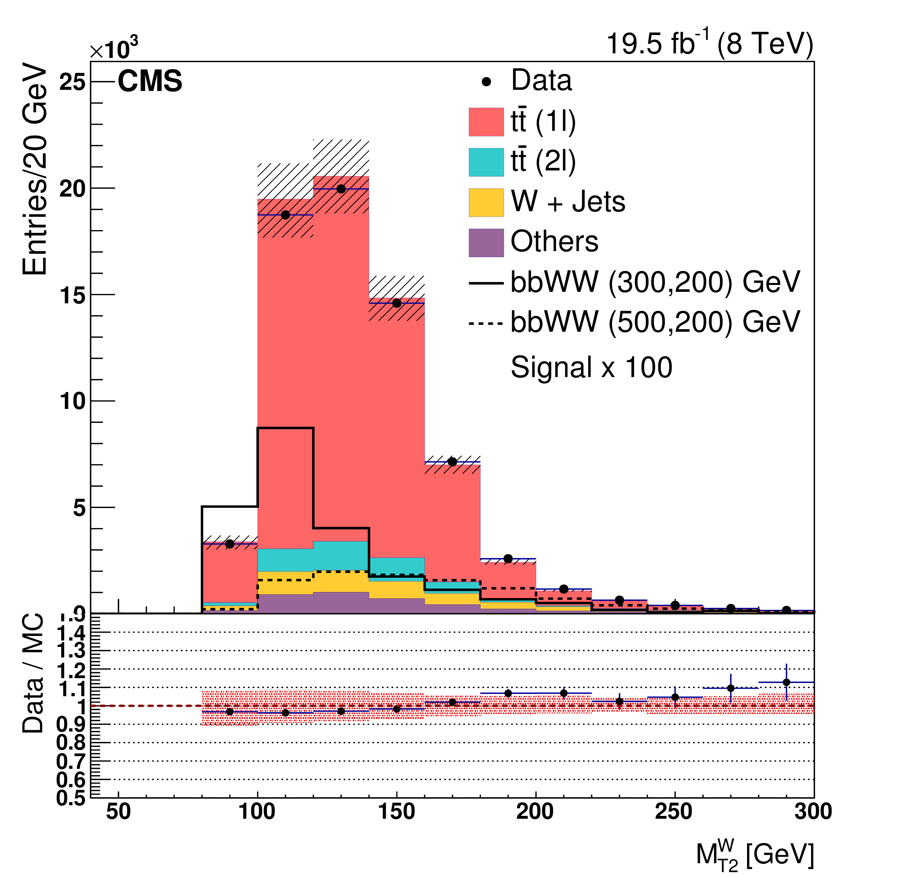
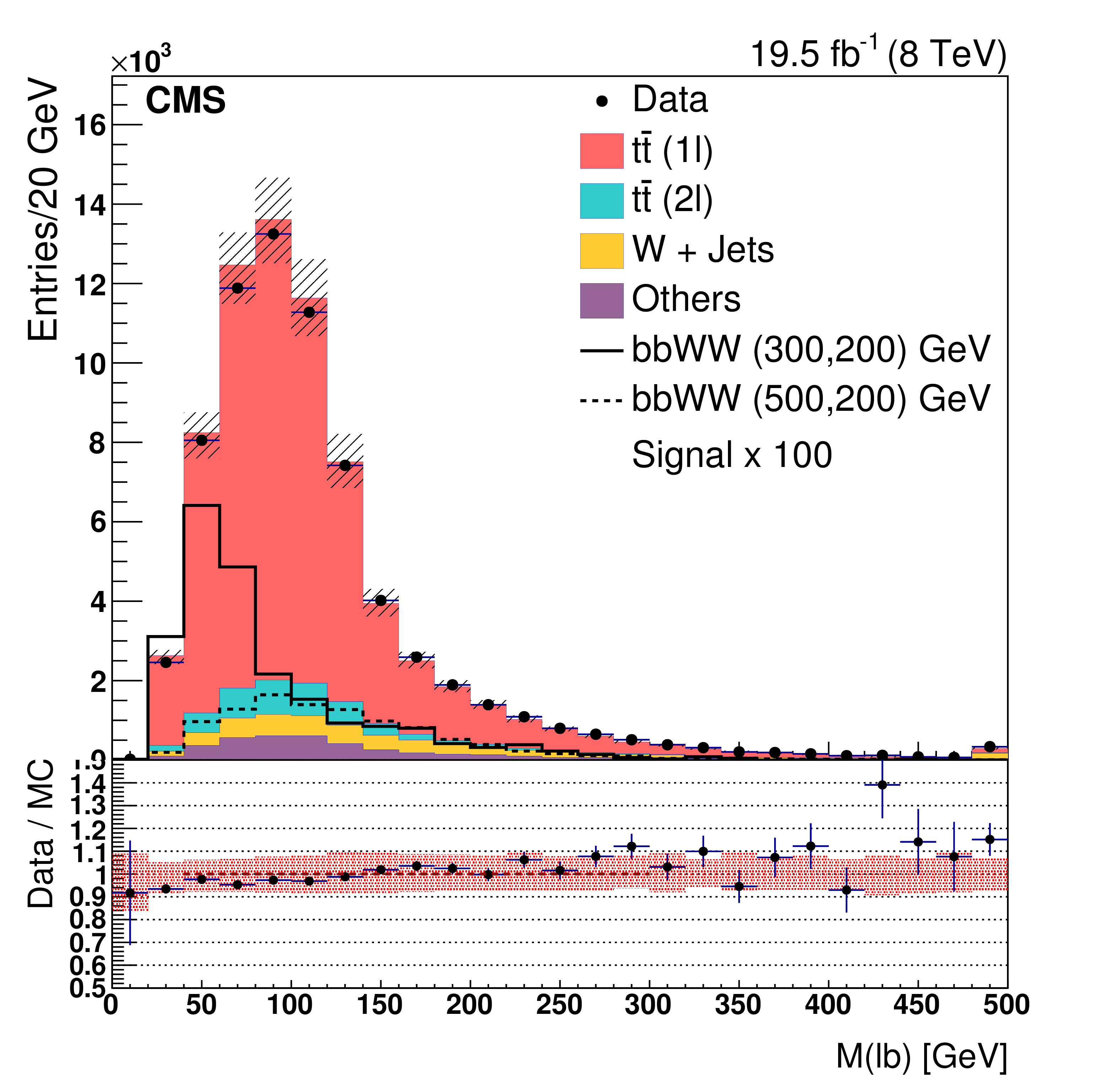
Figure 4-a:
Distributions of different variables in both data and simulation, for both e and $\mu $ final states at the preselection level without the ${M_{\mathrm {T}}}$ requirement. From (a,c) to (b,d): ${M_{{\mathrm T}2}^{ {\mathrm {W}}}} $, ${M(\text {3 jet})} $, ${M(\ell {\mathrm {b}})}$ and ${N(\text {jets})} $. The hatched region represents the quadratic sum of statistical and JES simulation uncertainties. The lower panel shows the ratio of data to total simulation background, with the red band representing the uncertainties mentioned in the text. Two signal mass points of the bbWW decay mode ($x=$ 0.75) are represented by open histograms, dashed and solid, with their cross sections scaled by 100; the two mass points ${ ( {{m}}( \tilde{ \mathrm{t} }_{1} ), {{m}}( { {\tilde{\chi}^{0}_{1}} } ) )}$ are (300, 200) and (500, 200) GeV. |
png pdf |
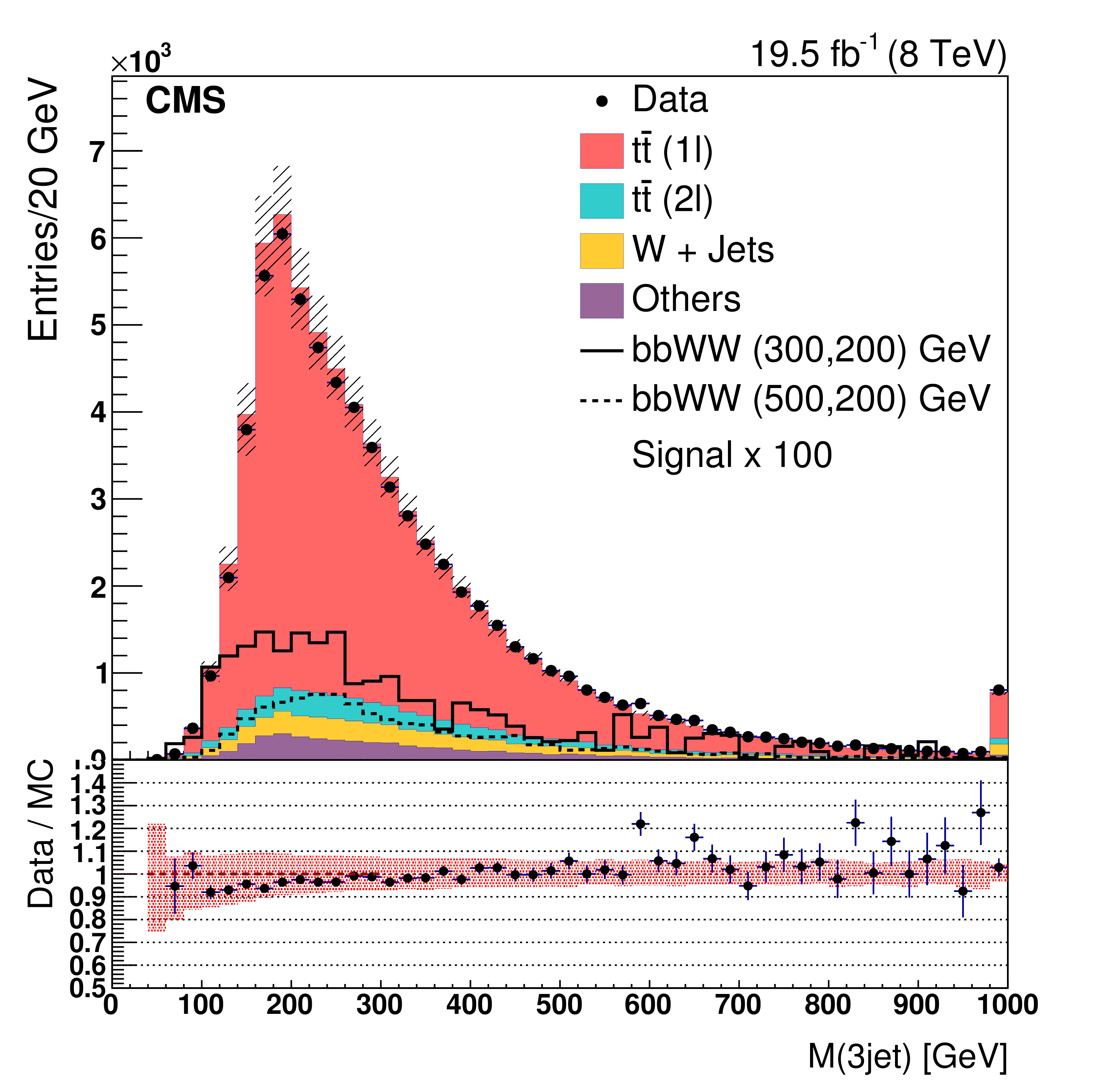
Figure 4-b:
Distributions of different variables in both data and simulation, for both e and $\mu $ final states at the preselection level without the ${M_{\mathrm {T}}}$ requirement. From (a,c) to (b,d): ${M_{{\mathrm T}2}^{ {\mathrm {W}}}} $, ${M(\text {3 jet})} $, ${M(\ell {\mathrm {b}})}$ and ${N(\text {jets})} $. The hatched region represents the quadratic sum of statistical and JES simulation uncertainties. The lower panel shows the ratio of data to total simulation background, with the red band representing the uncertainties mentioned in the text. Two signal mass points of the bbWW decay mode ($x=$ 0.75) are represented by open histograms, dashed and solid, with their cross sections scaled by 100; the two mass points ${ ( {{m}}( \tilde{ \mathrm{t} }_{1} ), {{m}}( { {\tilde{\chi}^{0}_{1}} } ) )}$ are (300, 200) and (500, 200) GeV. |
png pdf |
Figure 4-c:
Distributions of different variables in both data and simulation, for both e and $\mu $ final states at the preselection level without the ${M_{\mathrm {T}}}$ requirement. From (a,c) to (b,d): ${M_{{\mathrm T}2}^{ {\mathrm {W}}}} $, ${M(\text {3 jet})} $, ${M(\ell {\mathrm {b}})}$ and ${N(\text {jets})} $. The hatched region represents the quadratic sum of statistical and JES simulation uncertainties. The lower panel shows the ratio of data to total simulation background, with the red band representing the uncertainties mentioned in the text. Two signal mass points of the bbWW decay mode ($x=$ 0.75) are represented by open histograms, dashed and solid, with their cross sections scaled by 100; the two mass points ${ ( {{m}}( \tilde{ \mathrm{t} }_{1} ), {{m}}( { {\tilde{\chi}^{0}_{1}} } ) )}$ are (300, 200) and (500, 200) GeV. |
png pdf |
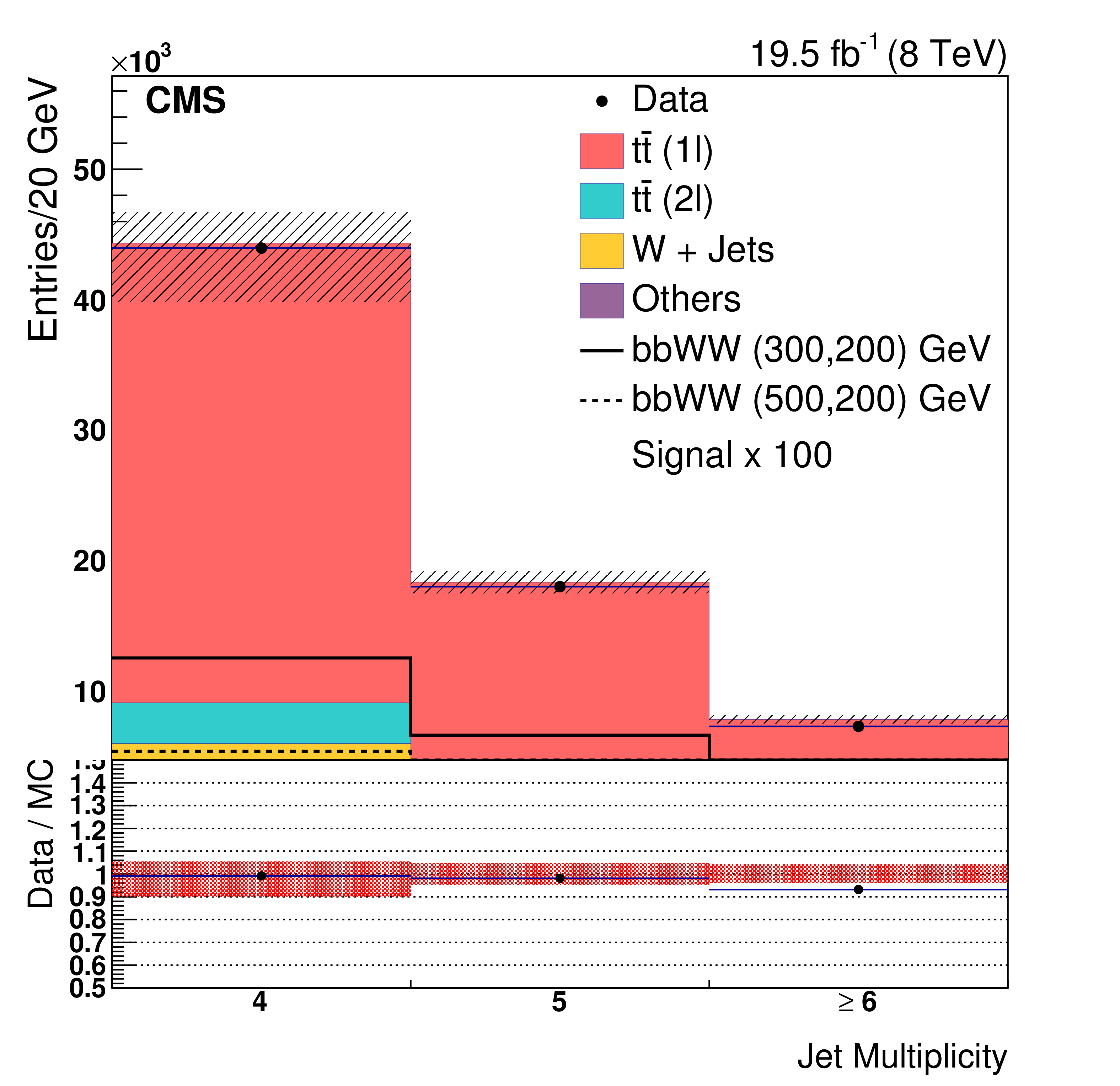
Figure 4-d:
Distributions of different variables in both data and simulation, for both e and $\mu $ final states at the preselection level without the ${M_{\mathrm {T}}}$ requirement. From (a,c) to (b,d): ${M_{{\mathrm T}2}^{ {\mathrm {W}}}} $, ${M(\text {3 jet})} $, ${M(\ell {\mathrm {b}})}$ and ${N(\text {jets})} $. The hatched region represents the quadratic sum of statistical and JES simulation uncertainties. The lower panel shows the ratio of data to total simulation background, with the red band representing the uncertainties mentioned in the text. Two signal mass points of the bbWW decay mode ($x=$ 0.75) are represented by open histograms, dashed and solid, with their cross sections scaled by 100; the two mass points ${ ( {{m}}( \tilde{ \mathrm{t} }_{1} ), {{m}}( { {\tilde{\chi}^{0}_{1}} } ) )}$ are (300, 200) and (500, 200) GeV. |
png pdf |
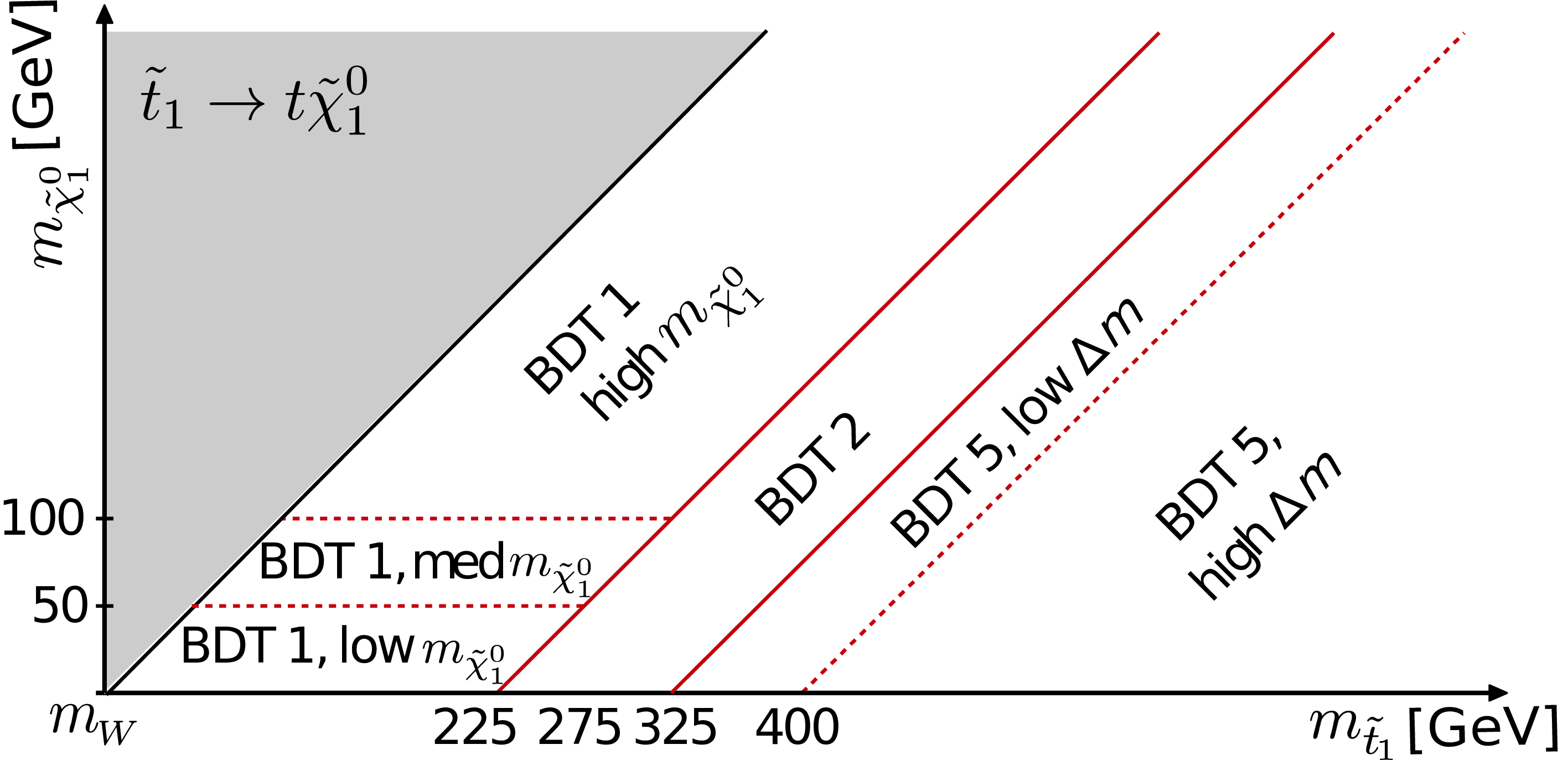
Figure 5-a:
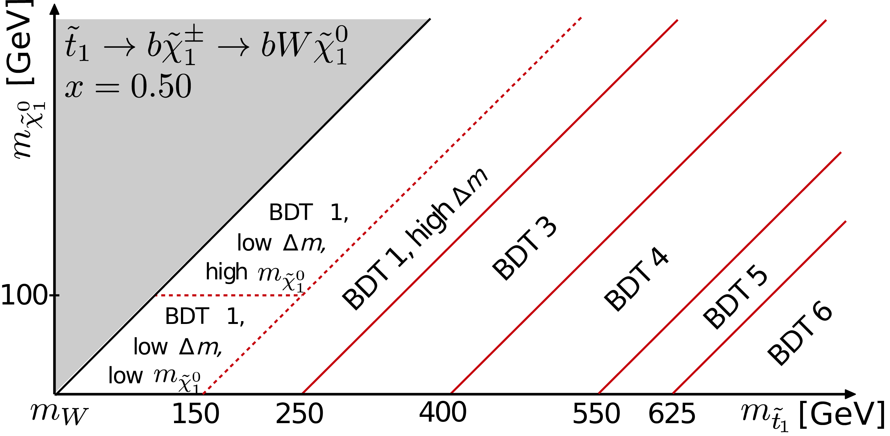
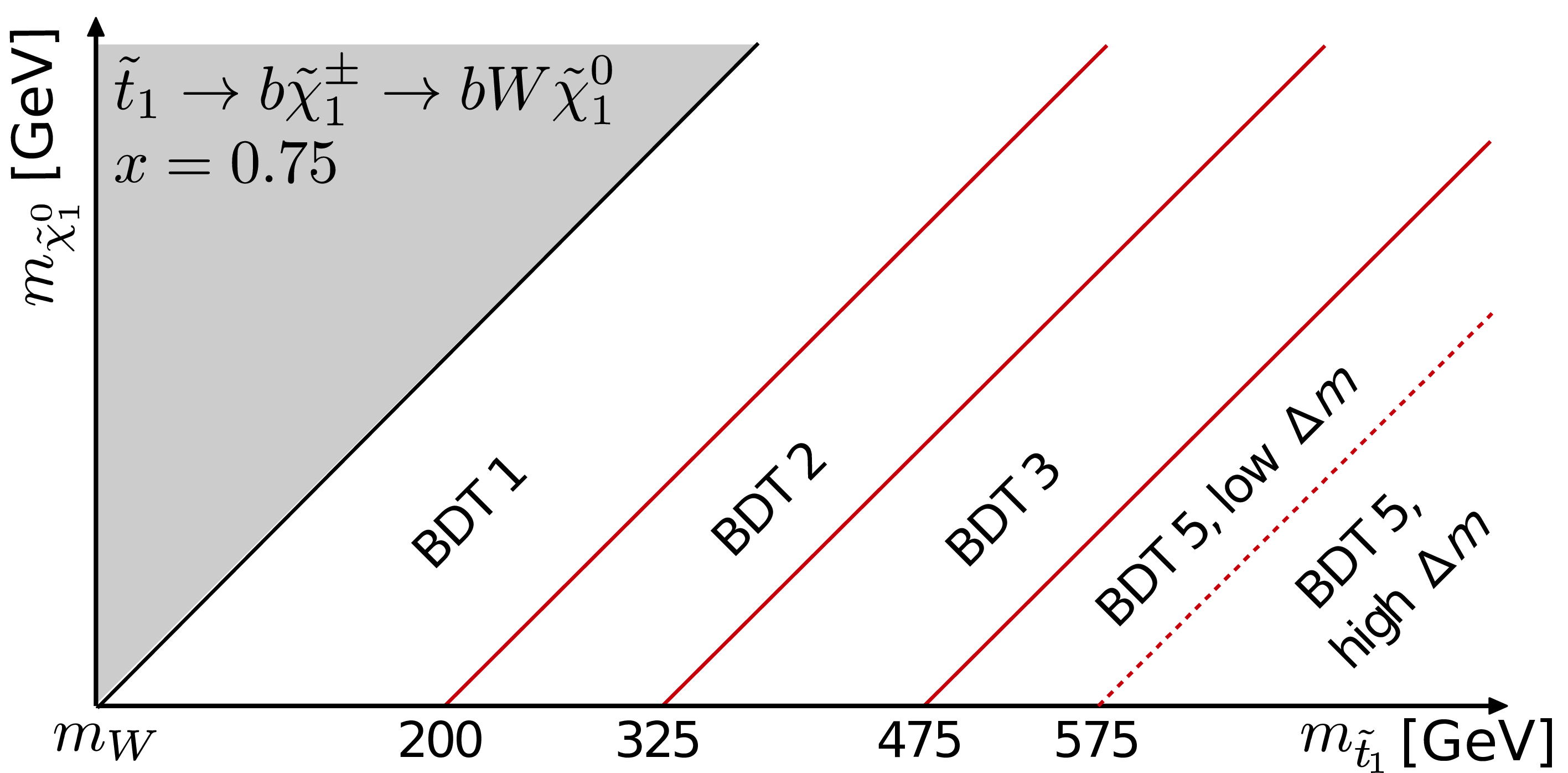
Signal regions (SRs) defined as functions of the chosen BDT trainings in the ${ ( {{m}}( \tilde{ \mathrm{t} }_{1} ), {{m}}( { {\tilde{\chi}^{0}_{1}} } ) )}$ plane for tt (a), bbWW $x=$ 0.25 (b), 0.50 (c), and 0.75 (d) decay modes. The SRs are delimited by continuous red lines, and the final selections within the different SRs are delimited by dashed red lines. The attributes ``low / high $m( { {\tilde{\chi}^{0}_{1}} } )$'' and ``low / high ${\Delta m} $'' indicate that in these regions different thresholds are applied for the same BDT training. |
png pdf |
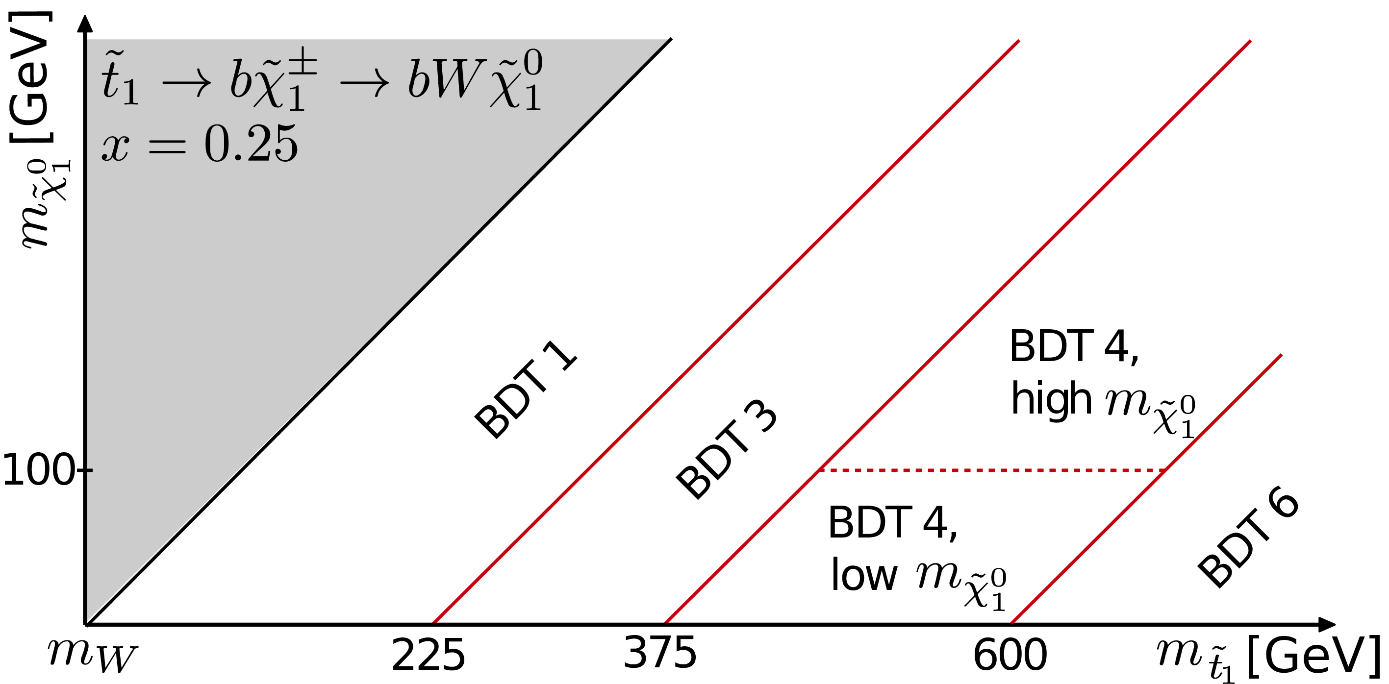
Figure 5-b:
Signal regions (SRs) defined as functions of the chosen BDT trainings in the ${ ( {{m}}( \tilde{ \mathrm{t} }_{1} ), {{m}}( { {\tilde{\chi}^{0}_{1}} } ) )}$ plane for tt (a), bbWW $x=$ 0.25 (b), 0.50 (c), and 0.75 (d) decay modes. The SRs are delimited by continuous red lines, and the final selections within the different SRs are delimited by dashed red lines. The attributes ``low / high $m( { {\tilde{\chi}^{0}_{1}} } )$'' and ``low / high ${\Delta m} $'' indicate that in these regions different thresholds are applied for the same BDT training. |
png pdf |
Figure 5-c:
Signal regions (SRs) defined as functions of the chosen BDT trainings in the ${ ( {{m}}( \tilde{ \mathrm{t} }_{1} ), {{m}}( { {\tilde{\chi}^{0}_{1}} } ) )}$ plane for tt (a), bbWW $x=$ 0.25 (b), 0.50 (c), and 0.75 (d) decay modes. The SRs are delimited by continuous red lines, and the final selections within the different SRs are delimited by dashed red lines. The attributes ``low / high $m( { {\tilde{\chi}^{0}_{1}} } )$'' and ``low / high ${\Delta m} $'' indicate that in these regions different thresholds are applied for the same BDT training. |
png pdf |
Figure 5-d:
Signal regions (SRs) defined as functions of the chosen BDT trainings in the ${ ( {{m}}( \tilde{ \mathrm{t} }_{1} ), {{m}}( { {\tilde{\chi}^{0}_{1}} } ) )}$ plane for tt (a), bbWW $x=$ 0.25 (b), 0.50 (c), and 0.75 (d) decay modes. The SRs are delimited by continuous red lines, and the final selections within the different SRs are delimited by dashed red lines. The attributes ``low / high $m( { {\tilde{\chi}^{0}_{1}} } )$'' and ``low / high ${\Delta m} $'' indicate that in these regions different thresholds are applied for the same BDT training. |
png pdf |
Figure 6-a:
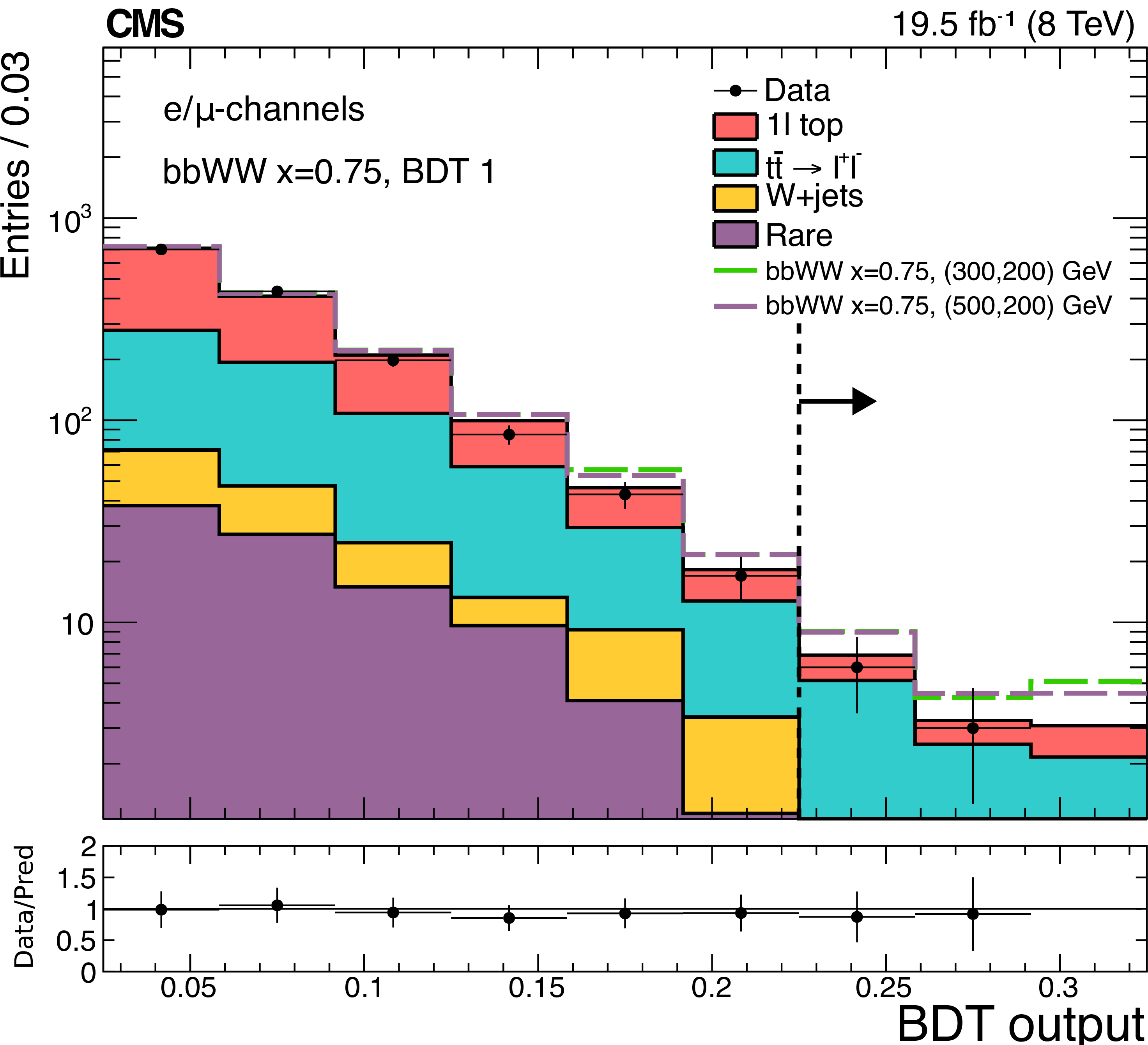
The BDT output distributions of the bbWW ($x=$ 0.75) decay mode in both final states at the preselection level for data and predicted background, with $\mathrm {BDT1} >$ 0.025 (a) and $\mathrm {BDT5}>$ 0 (b). Two representative signal mass points are shown: $ { ( {{m}}( \tilde{ \mathrm{t} }_{1} ), {{m}}( { {\tilde{\chi}^{0}_{1}} } ) )} =$ (300,200) and (500,200) GeV. In each panel the final selection is indicated by the vertical black dashed line. The normalization and $ {M_{\mathrm {T}}}$ correction (see Section 4.2.2), computed in the tail of the BDT output, i.e. to the right of the dashed line, are here propagated to the full distribution. The uncertainties are statistical. The plots on the bottom represent the ratio of Data over the predicted background, where we quadratically add statistical uncertainties with the uncertainties on the scale factors. |

png pdf |
Figure 6-b:
The BDT output distributions of the bbWW ($x=$ 0.75) decay mode in both final states at the preselection level for data and predicted background, with $\mathrm {BDT1} >$ 0.025 (a) and $\mathrm {BDT5}>$ 0 (b). Two representative signal mass points are shown: $ { ( {{m}}( \tilde{ \mathrm{t} }_{1} ), {{m}}( { {\tilde{\chi}^{0}_{1}} } ) )} =$ (300,200) and (500,200) GeV. In each panel the final selection is indicated by the vertical black dashed line. The normalization and $ {M_{\mathrm {T}}}$ correction (see Section 4.2.2), computed in the tail of the BDT output, i.e. to the right of the dashed line, are here propagated to the full distribution. The uncertainties are statistical. The plots on the bottom represent the ratio of Data over the predicted background, where we quadratically add statistical uncertainties with the uncertainties on the scale factors. |
png pdf |
Figure 7-a:
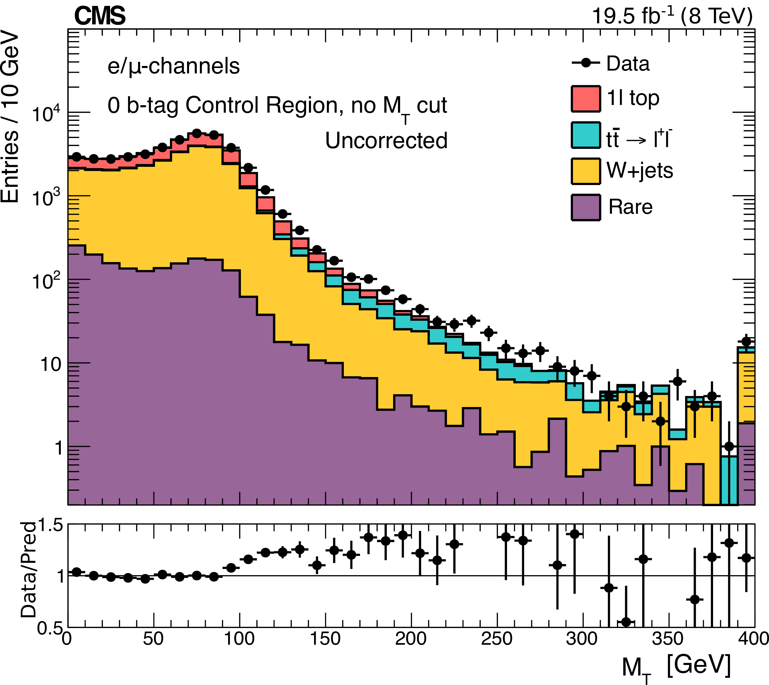
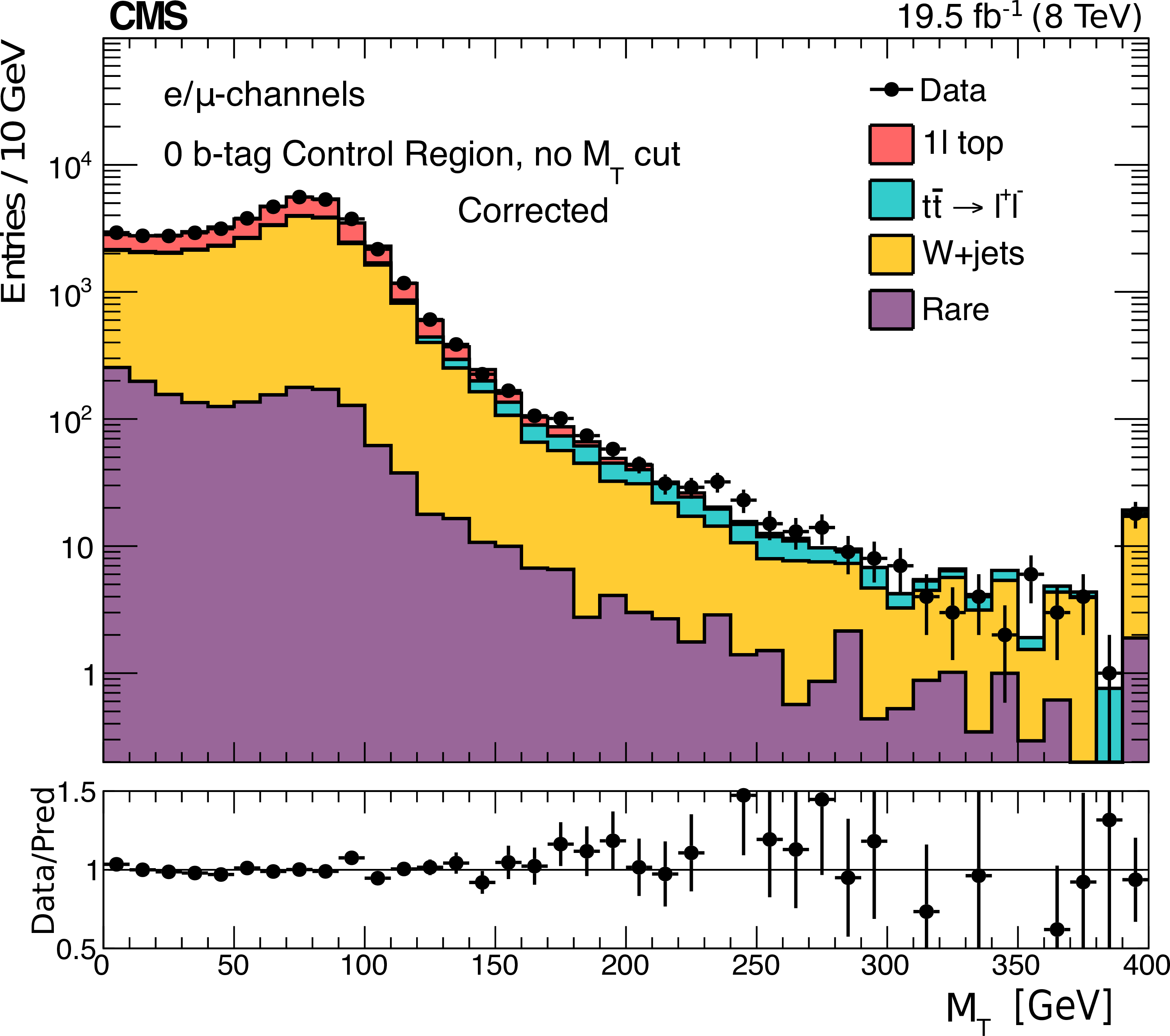
Full ${M_{\mathrm {T}}}$ distribution in the control region with zero b jets, without any extra signal selection. a: without the tail correction factors applied; b: with $SFR_{ {\mathrm {W}}}$ and $SFR_{\text {1$\ell $}}$ corrections applied. The plots on the bottom represent the ratio of Data over the predicted background. |
png pdf |
Figure 7-b:
Full ${M_{\mathrm {T}}}$ distribution in the control region with zero b jets, without any extra signal selection. a: without the tail correction factors applied; b: with $SFR_{ {\mathrm {W}}}$ and $SFR_{\text {1$\ell $}}$ corrections applied. The plots on the bottom represent the ratio of Data over the predicted background. |
png pdf |
Figure 8-a:
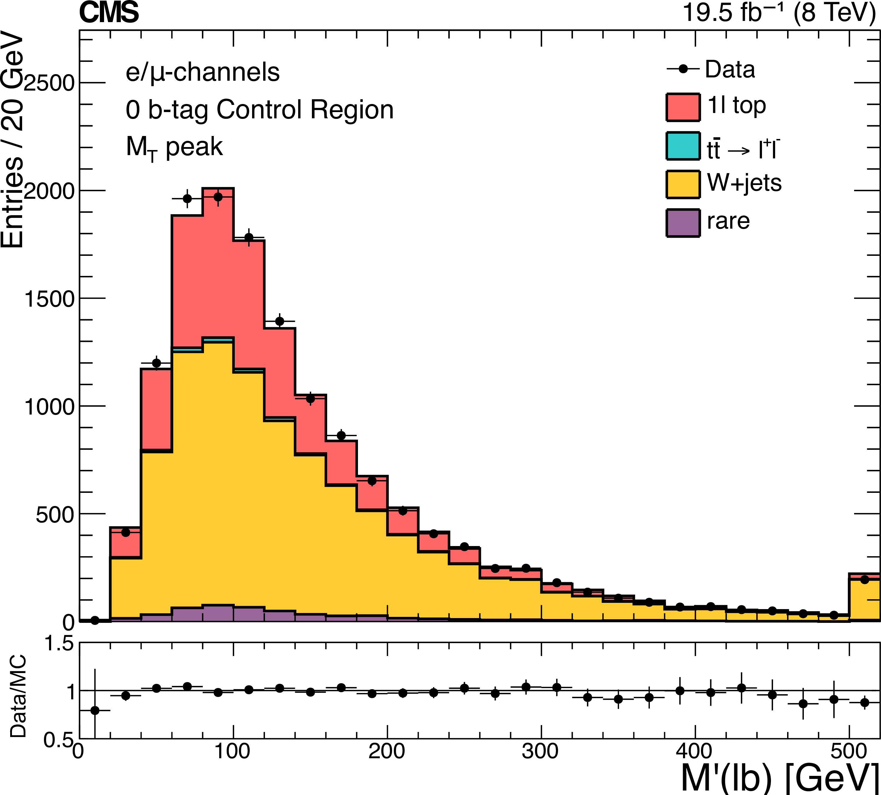
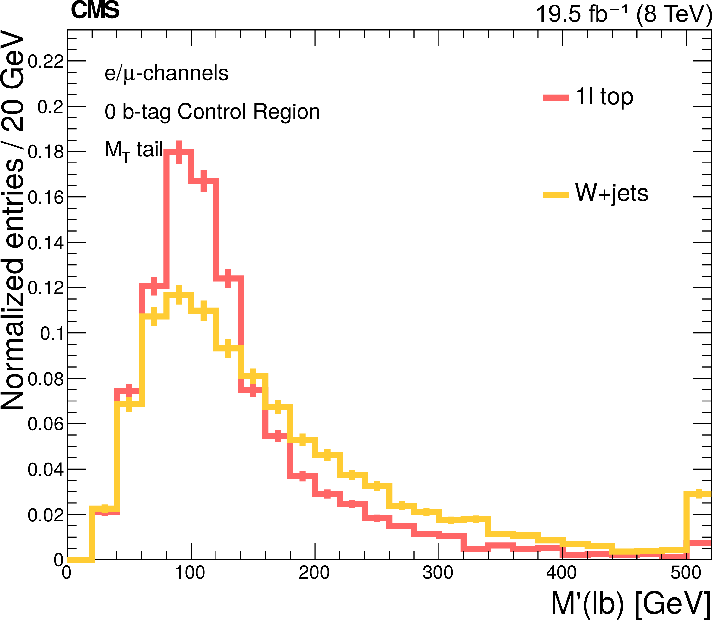
a: Comparison of data and simulation in the ${M^\prime _{\ell {\mathrm {b}}}}$ distributions for events with 50 $ < {M_{\mathrm {T}}} < $ 8 GeV and zero b jets. b: Shape comparison between ${ {\mathrm {t}\overline {\mathrm {t}}} \to 1\ell }$ and W+jets for $ {M_{\mathrm {T}}} > $ 100 GeV. |
png pdf |
Figure 8-b:
a: Comparison of data and simulation in the ${M^\prime _{\ell {\mathrm {b}}}}$ distributions for events with 50 $ < {M_{\mathrm {T}}} < $ 8 GeV and zero b jets. b: Shape comparison between ${ {\mathrm {t}\overline {\mathrm {t}}} \to 1\ell }$ and W+jets for $ {M_{\mathrm {T}}} > $ 100 GeV. |

png pdf |
Figure 9:
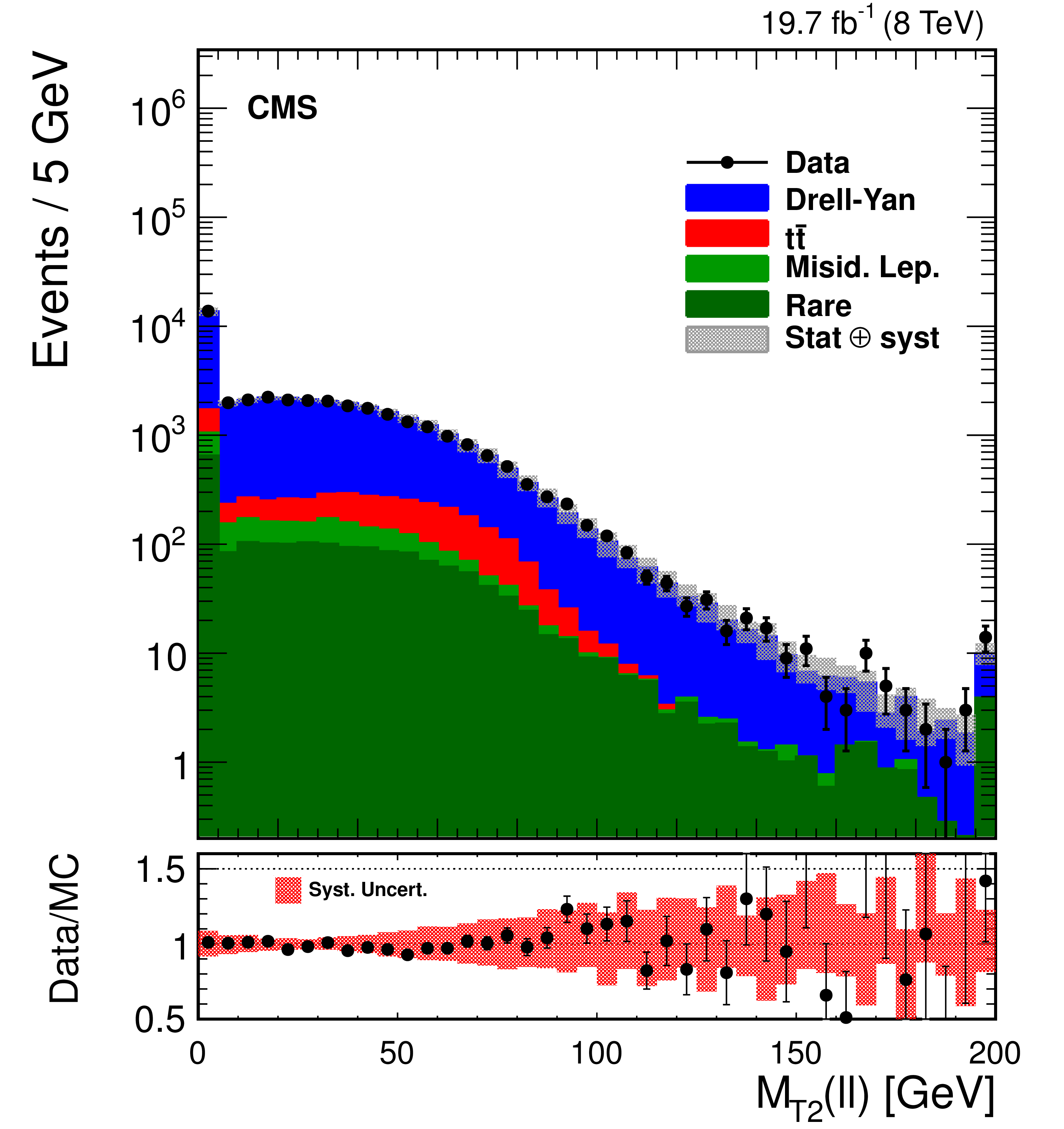
a: Data, expected background, and signal contributions in the ${M_{\mathrm {T2}}^{\ell \ell }}$ distribution at the preselection level. Background processes are estimated as in Section 5.2. The uncertainty bands are calculated from the full list of uncertainties discussed in Section 5.4. The same signal mass point $ { ( {{m}}( \tilde{ \mathrm{t} }_{1} ), {{m}}( { {\tilde{\chi}^{0}_{1}} } ) )} =$ (400,50) GeV is represented for the tt and bbWW ($x=$ 0.75) decay modes. b: ${M_{\mathrm {T2}}^{\ell \ell }}$ distribution for the $ {\mathrm {t}\overline {\mathrm {t}}} $ background and different signal mass points of the tt decay mode regrouped in constant $\Delta m$ bands; distributions are normalized to the same area. |
png pdf |
Figure 9-a:
a: Data, expected background, and signal contributions in the ${M_{\mathrm {T2}}^{\ell \ell }}$ distribution at the preselection level. Background processes are estimated as in Section 5.2. The uncertainty bands are calculated from the full list of uncertainties discussed in Section 5.4. The same signal mass point $ { ( {{m}}( \tilde{ \mathrm{t} }_{1} ), {{m}}( { {\tilde{\chi}^{0}_{1}} } ) )} =$ (400,50) GeV is represented for the tt and bbWW ($x=$ 0.75) decay modes. b: ${M_{\mathrm {T2}}^{\ell \ell }}$ distribution for the $ {\mathrm {t}\overline {\mathrm {t}}} $ background and different signal mass points of the tt decay mode regrouped in constant $\Delta m$ bands; distributions are normalized to the same area. |

png pdf |
Figure 9-b:
a: Data, expected background, and signal contributions in the ${M_{\mathrm {T2}}^{\ell \ell }}$ distribution at the preselection level. Background processes are estimated as in Section 5.2. The uncertainty bands are calculated from the full list of uncertainties discussed in Section 5.4. The same signal mass point $ { ( {{m}}( \tilde{ \mathrm{t} }_{1} ), {{m}}( { {\tilde{\chi}^{0}_{1}} } ) )} =$ (400,50) GeV is represented for the tt and bbWW ($x=$ 0.75) decay modes. b: ${M_{\mathrm {T2}}^{\ell \ell }}$ distribution for the $ {\mathrm {t}\overline {\mathrm {t}}} $ background and different signal mass points of the tt decay mode regrouped in constant $\Delta m$ bands; distributions are normalized to the same area. |
png pdf |
Figure 10:
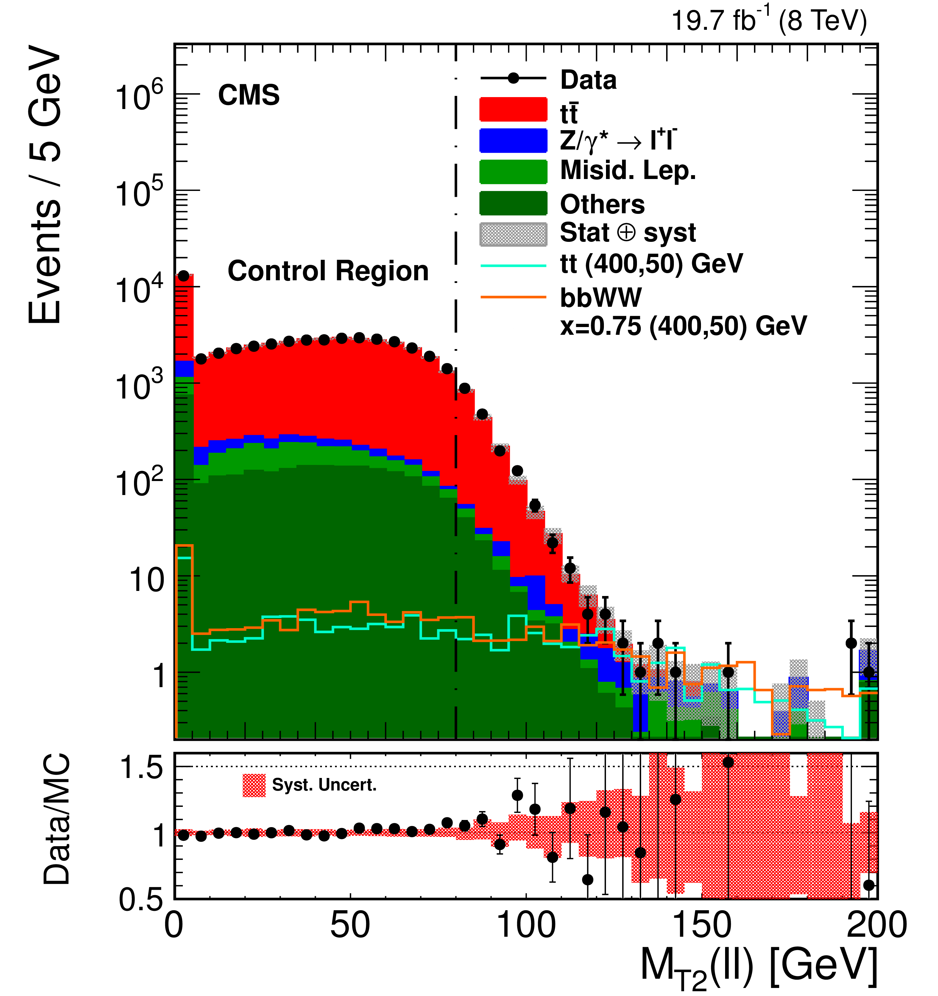
Data and expected background contributions for the ${M_{\mathrm {T2}}^{\ell \ell }}$ distribution in a control region enriched in $\mathrm{Z} \to \ell \ell $ events. This control region is similar to the preselection, except that the Z boson veto and b jet requirements have been inverted. Background processes are estimated as in Section 5.2. The uncertainty bands are calculated from the full list of uncertainties discussed in Section 5.4. |
png pdf |
Figure 10-a:
Data and expected background contributions for the ${M_{\mathrm {T2}}^{\ell \ell }}$ distribution in a control region enriched in $\mathrm{Z} \to \ell \ell $ events. This control region is similar to the preselection, except that the Z boson veto and b jet requirements have been inverted. Background processes are estimated as in Section 5.2. The uncertainty bands are calculated from the full list of uncertainties discussed in Section 5.4. |

png pdf |
Figure 10-b:
Data and expected background contributions for the ${M_{\mathrm {T2}}^{\ell \ell }}$ distribution in a control region enriched in $\mathrm{Z} \to \ell \ell $ events. This control region is similar to the preselection, except that the Z boson veto and b jet requirements have been inverted. Background processes are estimated as in Section 5.2. The uncertainty bands are calculated from the full list of uncertainties discussed in Section 5.4. |
png pdf |
Figure 10-c:
Data and expected background contributions for the ${M_{\mathrm {T2}}^{\ell \ell }}$ distribution in a control region enriched in $\mathrm{Z} \to \ell \ell $ events. This control region is similar to the preselection, except that the Z boson veto and b jet requirements have been inverted. Background processes are estimated as in Section 5.2. The uncertainty bands are calculated from the full list of uncertainties discussed in Section 5.4. |
png pdf |
Figure 10-d:
Data and expected background contributions for the ${M_{\mathrm {T2}}^{\ell \ell }}$ distribution in a control region enriched in $\mathrm{Z} \to \ell \ell $ events. This control region is similar to the preselection, except that the Z boson veto and b jet requirements have been inverted. Background processes are estimated as in Section 5.2. The uncertainty bands are calculated from the full list of uncertainties discussed in Section 5.4. |

png pdf |
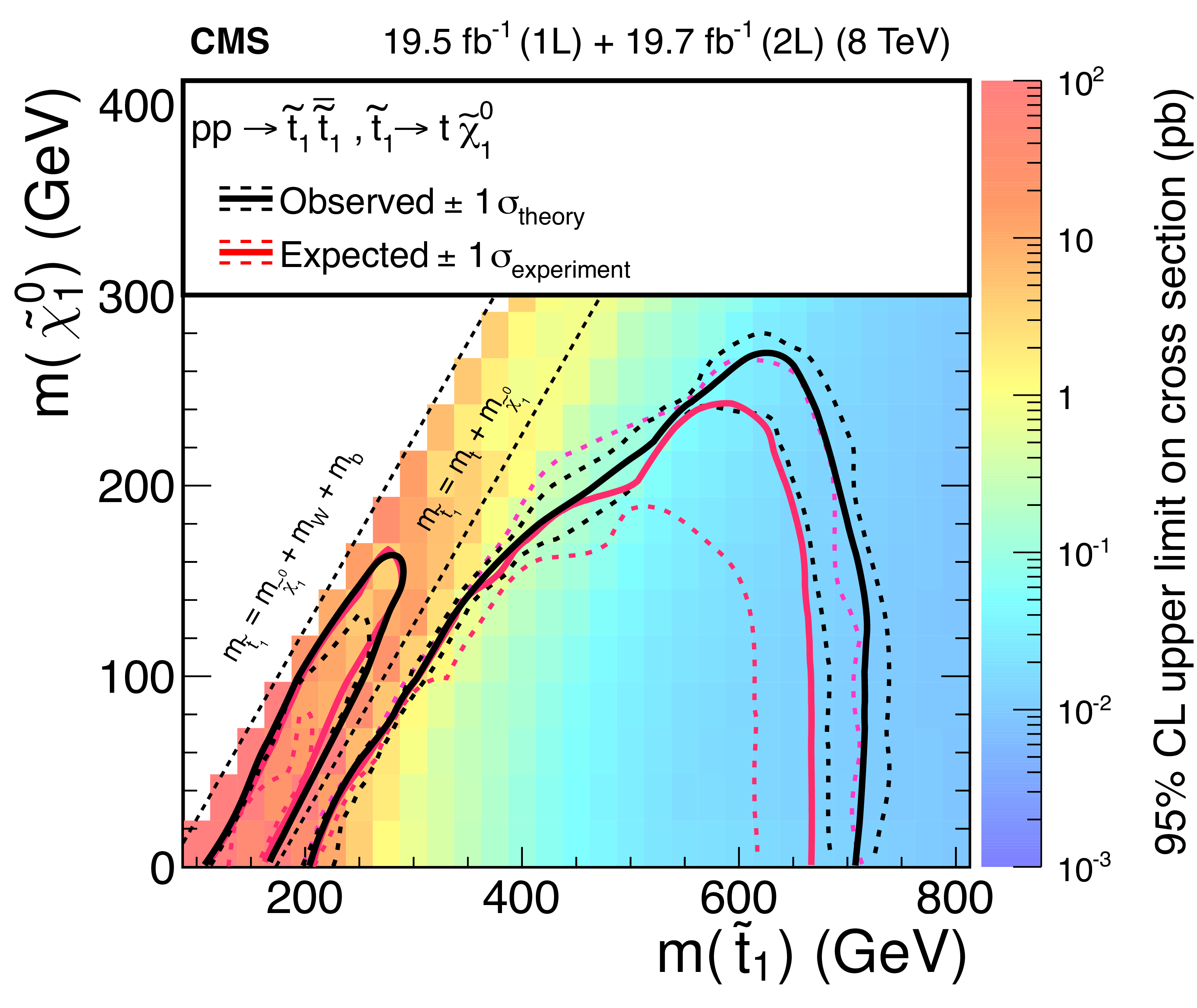
Figure 11-a:
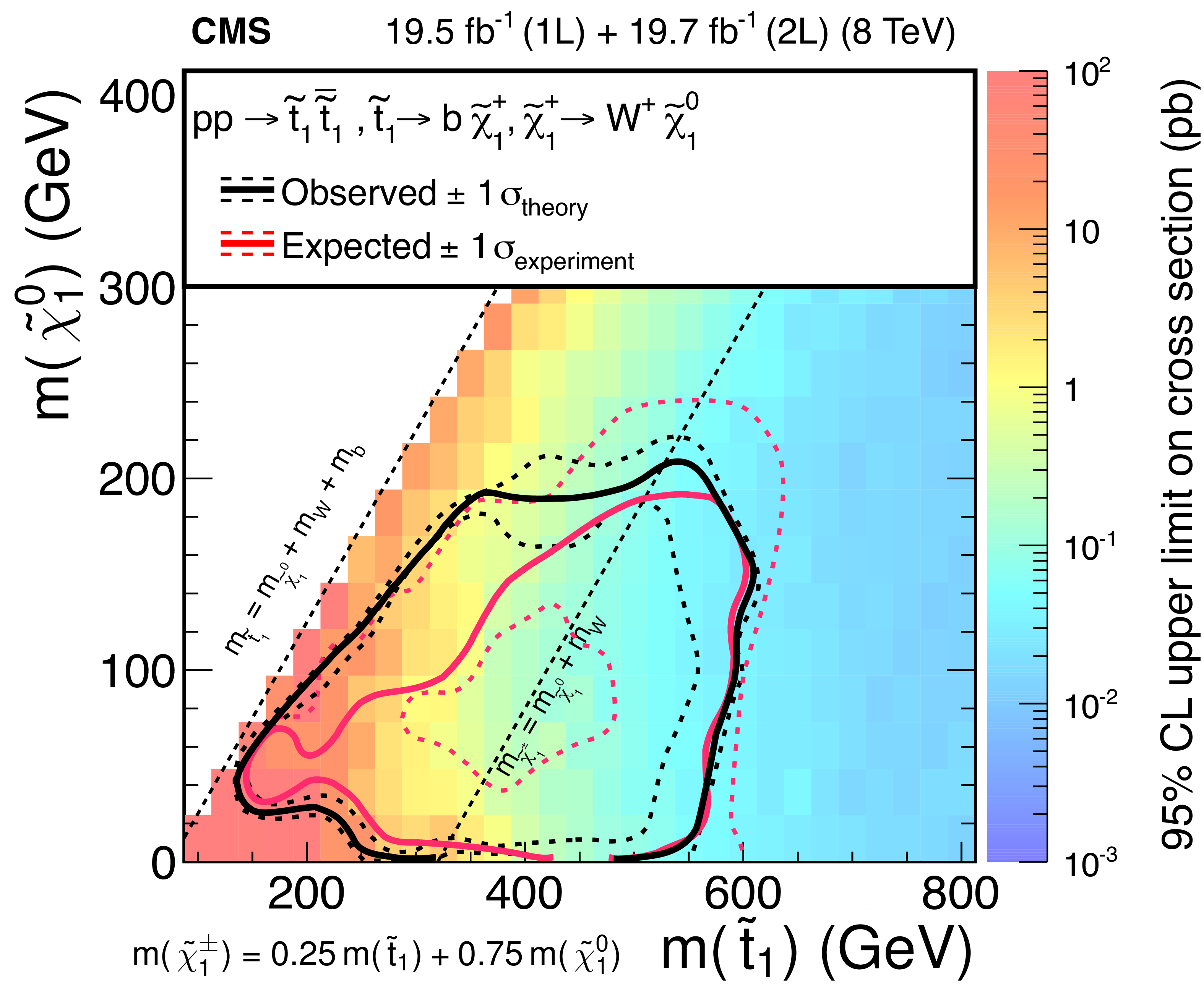
Exclusion limit at 95% CL obtained with a statistical combination of the results from the single-lepton and dilepton searches, for the tt (a), bbWW $x=$ 0.25 (b), bbWW $x=$ 0.50 (c) and bbWW $x=$ 0.75 (d) decay modes. The red and black lines represent the expected and observed limits, respectively; the dotted lines represent in each case the $\pm $1$\sigma $ variations of the contours. For all decay modes, we show the kinematic limit $m( \tilde{ \mathrm{t} }_{1} )=m( {\mathrm {b}})+m( {\mathrm {W}})+m( { {\tilde{\chi}^{0}_{1}} } )$ on the left side of the $(m( \tilde{ \mathrm{t} }_{1} ),m( { {\tilde{\chi}^{0}_{1}} } ))$ plane; for the tt decay mode, we show the $ {\Delta m} =m( {\mathrm {t}})$ line; and for the bbWW decay mode, we show the $m( {\tilde{\chi}^\pm _{1}} )-m( { {\tilde{\chi}^{0}_{1}} } )=m( {\mathrm {W}})$ line. |
png pdf |
Figure 11-b:
Exclusion limit at 95% CL obtained with a statistical combination of the results from the single-lepton and dilepton searches, for the tt (a), bbWW $x=$ 0.25 (b), bbWW $x=$ 0.50 (c) and bbWW $x=$ 0.75 (d) decay modes. The red and black lines represent the expected and observed limits, respectively; the dotted lines represent in each case the $\pm $1$\sigma $ variations of the contours. For all decay modes, we show the kinematic limit $m( \tilde{ \mathrm{t} }_{1} )=m( {\mathrm {b}})+m( {\mathrm {W}})+m( { {\tilde{\chi}^{0}_{1}} } )$ on the left side of the $(m( \tilde{ \mathrm{t} }_{1} ),m( { {\tilde{\chi}^{0}_{1}} } ))$ plane; for the tt decay mode, we show the $ {\Delta m} =m( {\mathrm {t}})$ line; and for the bbWW decay mode, we show the $m( {\tilde{\chi}^\pm _{1}} )-m( { {\tilde{\chi}^{0}_{1}} } )=m( {\mathrm {W}})$ line. |

png pdf |
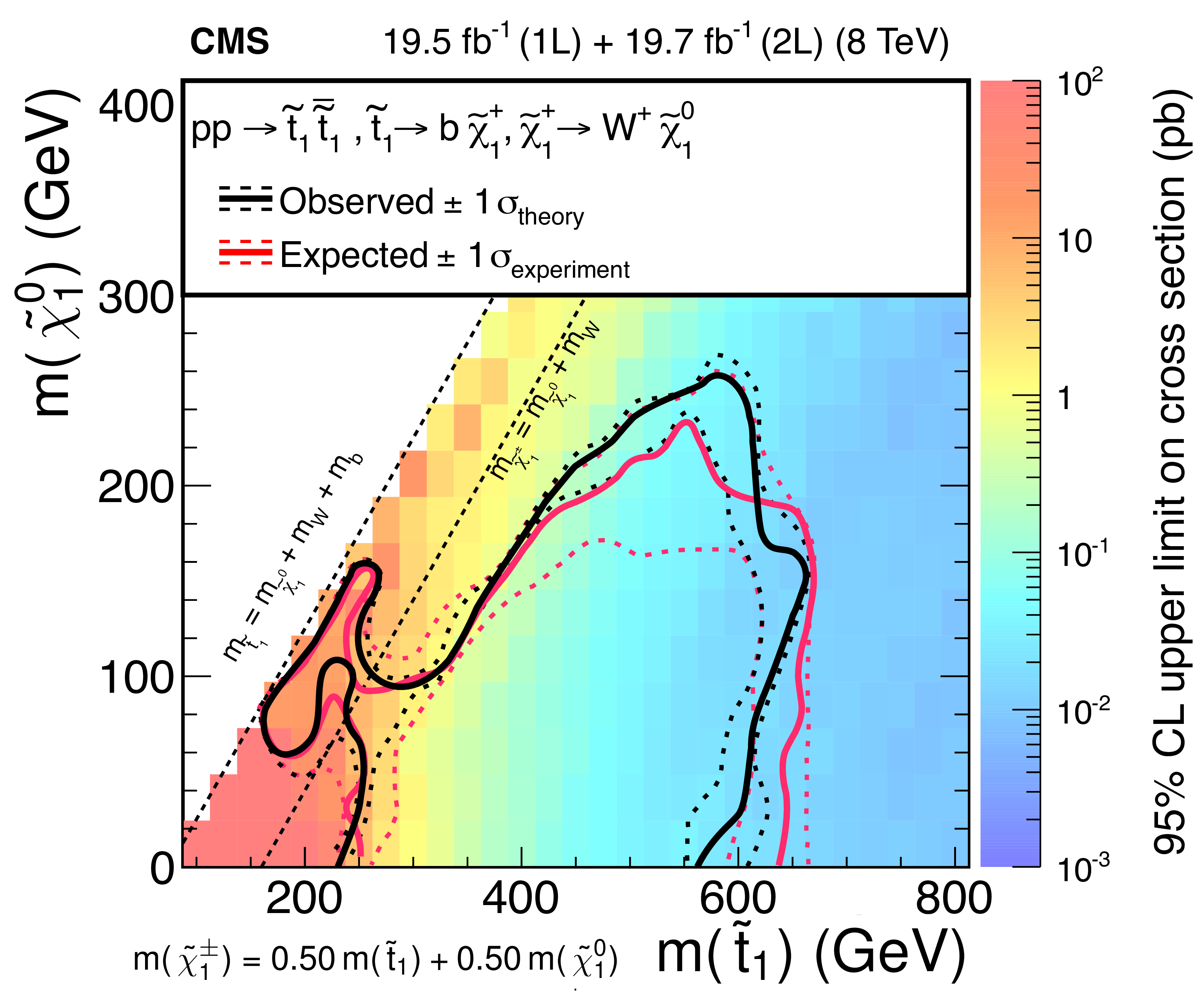
Figure 11-c:
Exclusion limit at 95% CL obtained with a statistical combination of the results from the single-lepton and dilepton searches, for the tt (a), bbWW $x=$ 0.25 (b), bbWW $x=$ 0.50 (c) and bbWW $x=$ 0.75 (d) decay modes. The red and black lines represent the expected and observed limits, respectively; the dotted lines represent in each case the $\pm $1$\sigma $ variations of the contours. For all decay modes, we show the kinematic limit $m( \tilde{ \mathrm{t} }_{1} )=m( {\mathrm {b}})+m( {\mathrm {W}})+m( { {\tilde{\chi}^{0}_{1}} } )$ on the left side of the $(m( \tilde{ \mathrm{t} }_{1} ),m( { {\tilde{\chi}^{0}_{1}} } ))$ plane; for the tt decay mode, we show the $ {\Delta m} =m( {\mathrm {t}})$ line; and for the bbWW decay mode, we show the $m( {\tilde{\chi}^\pm _{1}} )-m( { {\tilde{\chi}^{0}_{1}} } )=m( {\mathrm {W}})$ line. |

png pdf |
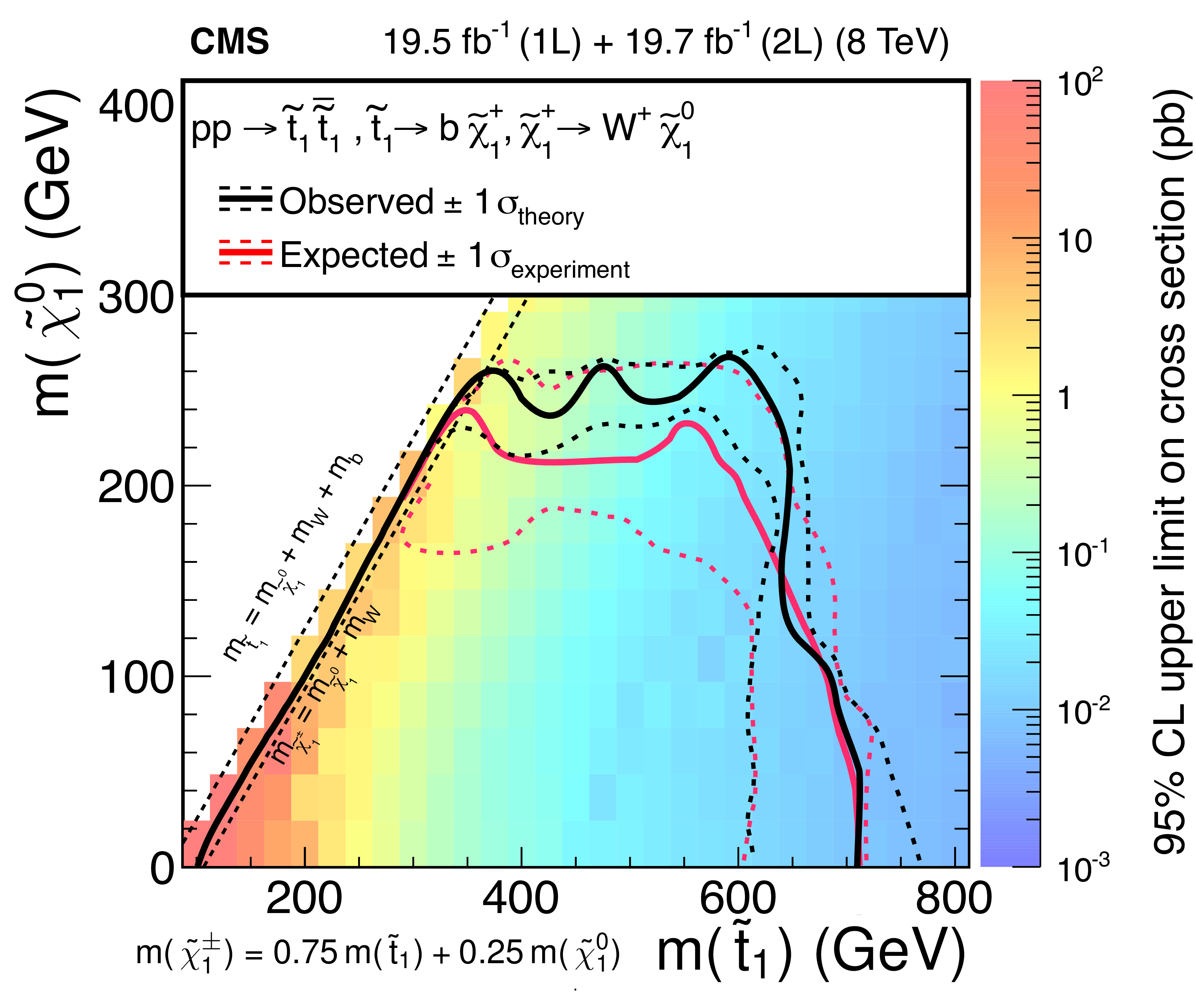
Figure 11-d:
Exclusion limit at 95% CL obtained with a statistical combination of the results from the single-lepton and dilepton searches, for the tt (a), bbWW $x=$ 0.25 (b), bbWW $x=$ 0.50 (c) and bbWW $x=$ 0.75 (d) decay modes. The red and black lines represent the expected and observed limits, respectively; the dotted lines represent in each case the $\pm $1$\sigma $ variations of the contours. For all decay modes, we show the kinematic limit $m( \tilde{ \mathrm{t} }_{1} )=m( {\mathrm {b}})+m( {\mathrm {W}})+m( { {\tilde{\chi}^{0}_{1}} } )$ on the left side of the $(m( \tilde{ \mathrm{t} }_{1} ),m( { {\tilde{\chi}^{0}_{1}} } ))$ plane; for the tt decay mode, we show the $ {\Delta m} =m( {\mathrm {t}})$ line; and for the bbWW decay mode, we show the $m( {\tilde{\chi}^\pm _{1}} )-m( { {\tilde{\chi}^{0}_{1}} } )=m( {\mathrm {W}})$ line. |
| Tables | |
png pdf |
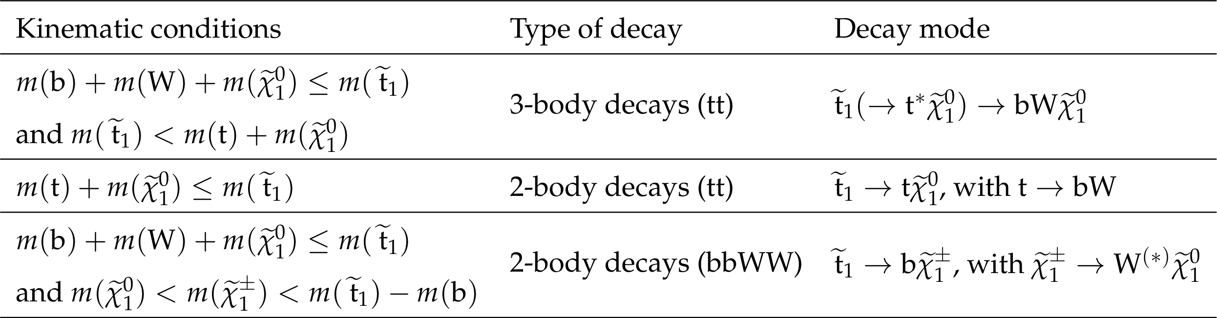
Table 1:
Kinematic conditions for the $ \tilde{ \mathrm{t} }_{1} $ decay modes explored in this paper. |
png pdf |
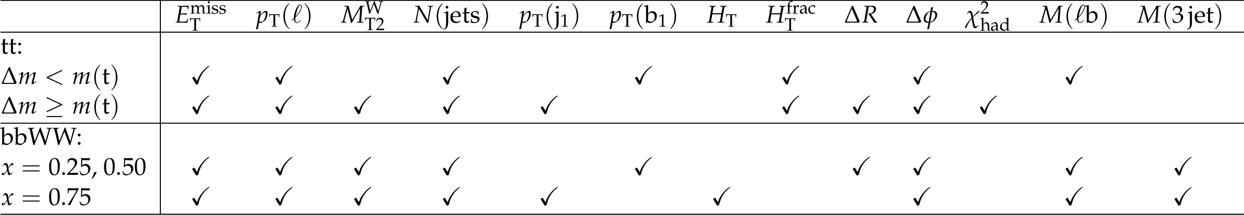
Table 2:
Final selection variables chosen as input for the BDT training, as functions of the decay modes bbWW and tt, and kinematic regions. Column headings ${\Delta R}$ and ${\Delta \phi }$ refer to ${\Delta R (\ell , {\mathrm {b}}_1)}$ and ${\Delta \phi (\mathrm {j}_{1,2}, {\vec{p}}_{\mathrm {T}}^{\text {miss}} )} $. |
png pdf |
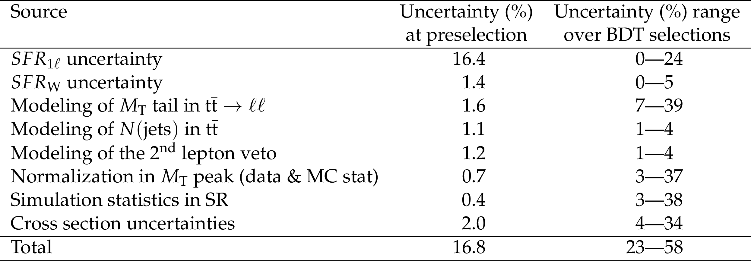
Table 3:
Summary of the relative systematic uncertainties in the total background, at the preselection level, and the range of variation over the BDT selections. |

png pdf |
Table 4:
Background prediction without signal contamination and observed data for the BDT selections. The total systematic uncertainties are reported for the predicted background. |
png pdf |
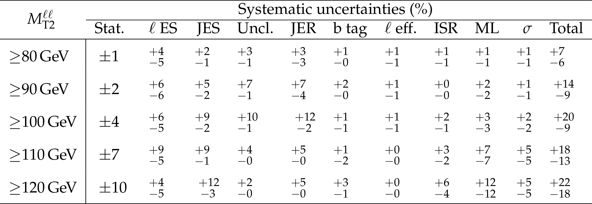
Table 5:
The relevant sources of systematic uncertainty in the background estimate for each signal region used in the limit setting. From left to right, the systematic uncertainty sources are: lepton energy scale ($\ell $ ES), jet energy scale (JES), unclustered energy scale (Uncl.), ${E_{\mathrm {T}}^{\text {miss}}}$ energy resolution from jets (JER), uncertainty in b tagging scale factors (b tag), lepton selection efficiency ($\ell $ eff.), ISR reweighting (ISR), the misidentified lepton estimate (ML), and the combined normalization uncertainty in the $ {\mathrm {t}\overline {\mathrm {t}}} $ , DY, and other electroweak backgrounds ($\sigma $). |
png pdf |
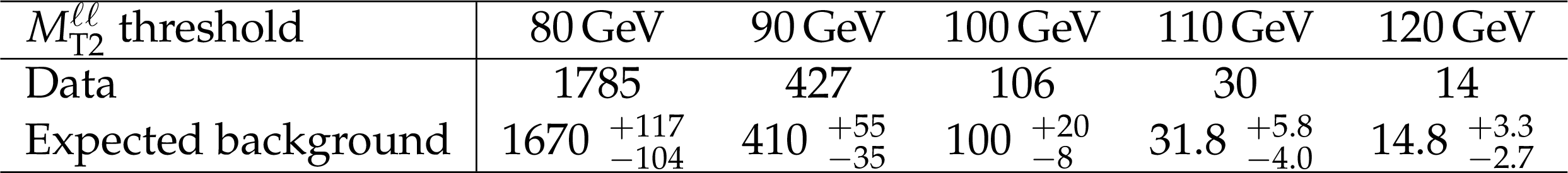
Table 6:
Data yields and background expectation for five different ${M_{\mathrm {T2}}^{\ell \ell }}$ threshold values. The asymmetric uncertainties quoted for the background indicate the total systematic uncertainty, including the statistical uncertainty in the background expectation. |
| Summary |
| Using up to 19.7 fb$^{-1}$ of pp collision data taken at $\sqrt{s}=$ 8 TeV, we search for direct top squark pair production in both single-lepton and dilepton final states. In both searches the standard model background, dominated by the $\mathrm{ t \bar{t} }$ process, is predicted using control samples in data. In this single-lepton search, we improve the results of Ref. [12] by employing an upgraded multivariate tool for signal selection, fed by both kinematic and topological variables and specifically trained for different decay modes and kinematic regions. This systematic approach to the signal selection, where the discriminating power of each selection variable is quantitatively assessed, is a key feature of the single-lepton search. The background determination method has also been improved compared to Ref. [12]. In the dilepton search the signal selection is based on the ${M_{\mathrm{T2}}}$ $S{\ell}{\ell}$ variable. In both searches, the effect of the signal contamination is accounted for. No excess above the predicted background is observed in either search. Simplified models (Fig. 1) are used to interpret the results in terms of a region in the ${ ( {{m}}( \tilde{ \mathrm{t} }_1), {{m}}({\tilde{\chi}^0_1} ) )}$ plane, excluded at 95% CL. We combine the results of both searches for maximal sensitivity; the sensitivity depends on the decay mode, and on the ${ ( {{m}}( \tilde{ \mathrm{t} }_1 ), {{m}}({\tilde{\chi}^0_1} ) )}$ signal point. The highest excluded $ \tilde{ \mathrm{t} }_1 $ and ${\tilde{\chi}^0_1} $ masses are about 700 GeV and 250 GeV, respectively. |
| References | ||||
| 1 | ATLAS Collaboration | Observation of a new particle in the search for the Standard Model Higgs boson with the ATLAS detector at the LHC | PLB 716 (2012) 1 | 1207.7214 |
| 2 | CMS Collaboration | Observation of a new boson at a mass of 125 GeV with the CMS experiment at the LHC | PLB 716 (2012) 30 | CMS-HIG-12-028 1207.7235 |
| 3 | CMS Collaboration | Combined results of searches for the standard model Higgs boson in $ pp $ collisions at $ \sqrt{s}=7 $ TeV | PLB 710 (2012) 26 | CMS-HIG-11-032 1202.1488 |
| 4 | C. Boehm, A. Djouadi, and M. Drees | Light scalar top quarks and supersymmetric dark matter | PRD 62 (2000) 035012 | hep-ph/9911496 |
| 5 | C. Bal\'azs, M. Carena, and C. E. M. Wagner | Dark matter, light stops and electroweak baryogenesis | PRD 70 (2004) 015007 | hep-ph/403224 |
| 6 | D0 Collaboration | Search for 3- and 4-body decays of the scalar top quark in $ \text{p}\bar{\text{p}} $ collisions at $ \sqrt{s} = 1.8 $ TeV | PLB 581 (2004) 147 | |
| 7 | D0 Collaboration | Search for pair production of the scalar top quark in muon+tau final states | PLB 710 (2012) 578 | 1202.1978 |
| 8 | D0 Collaboration | Search for the lightest scalar top quark in events with two leptons in $ \text{p}\bar{\text{p}} $ collisions at $ \sqrt{s} $ = 1.96-TeV | PLB 659 (2008) 500 | 0707.2864 |
| 9 | CDF Collaboration | Search for the supersymmetric partner of the top quark in $ \mathrm{p}\bar{\mathrm{p}} $ collisions at $ \sqrt{s} $ = 1.96 TeV | PRD 82 (2010) 092001 | 1009.0266 |
| 10 | CDF Collaboration | Search for the supersymmetric partner of the top quark in dilepton events from $ \mathrm{p}\bar{\mathrm{p}} $ collisions at $ \sqrt{s} = 1.8 $ TeV | PRL 90 (2003) 251801 | hep-ex/0302009 |
| 11 | ATLAS Collaboration | ATLAS Run 1 searches for direct pair production of third-generation squarks at the Large Hadron Collider | EPJC 75 (2015) 510 | 1506.08616 |
| 12 | CMS Collaboration | Search for top-squark pair production in the single-lepton final state in pp collisions at $ \sqrt{s} = 8 $ TeV | EPJC 73 (2013) 2677 | CMS-SUS-13-011 1308.1586 |
| 13 | M. Burns, K. Kong, K. T. Matchev, and M. Park | Using Subsystem MT2 for Complete Mass Determinations in Decay Chains with Missing Energy at Hadron Colliders | JHEP 03 (2009) 143 | 0810.5576 |
| 14 | CMS Collaboration | CMS. The TriDAS project. Technical design report, vol. 1: The trigger systems | CDS | |
| 15 | CMS Collaboration | The CMS experiment at the CERN LHC | JINST 3 (2008) S08004 | CMS-00-001 |
| 16 | CMS Collaboration | CMS Luminosity Based on Pixel Cluster Counting -- Summer 2013 Update | CMS-PAS-LUM-13-001 | CMS-PAS-LUM-13-001 |
| 17 | J. Alwall et al. | MadGraph 5: going beyond | JHEP 06 (2011) 128 | 1106.0522 |
| 18 | S. Frixione, P. Nason, and G. Ridolfi | A Positive-weight next-to-leading-order Monte Carlo for heavy flavour hadroproduction | JHEP 09 (2007) 126 | 0707.3088 |
| 19 | J. Pumplin et al. | New generation of parton distributions with uncertainties from global QCD analysis | JHEP 07 (2002) 012 | hep-ph/0201195 |
| 20 | H.-L. Lai et al. | New parton distributions for collider physics | PRD 82 (2010) 074024 | 1007.2241 |
| 21 | T. Sj\"ostrand, S. Mrenna, and P. Skands | PYTHIA 6.4 physics and manual | JHEP 05 (2006) 026 | hep-ph/0603175 |
| 22 | CMS Collaboration | Study of the underlying event at forward rapidity in pp collisions at $ \sqrt{s} = 0.9 $, 2.76, and 7$ TeV $ | JHEP 04 (2013) 072 | |
| 23 | GEANT4 Collaboration | GEANT4---a simulation toolkit | NIMA 506 (2003) 250 | |
| 24 | S. Abdullin et al. | The fast simulation of the CMS detector at LHC | in Intl. Conf. on Computing in High Energy and Nuclear Physics (CHEP 2010) 2012 J. Phys.: Conf. Ser. 331 (2012) 032049 | |
| 25 | W. Beenakker, R. Hopker, and M. Spira | PROSPINO: A Program for the production of supersymmetric particles in next-to-leading order QCD | hep-ph/9611232 | |
| 26 | W. Beenakker, R. H\"opker, M. Spira, and P. M. Zerwas | Squark and gluino production at hadron colliders | Nucl. Phys. B 492 (1997) 51 | hep-ph/9610490 |
| 27 | A. Kulesza and L. Motyka | Threshold resummation for squark-antisquark and gluino-pair production at the LHC | PRL 102 (2009) 111802 | hep-ph/0807.2405 |
| 28 | A. Kulesza and L. Motyka | Soft gluon resummation for the production of gluino-gluino and squark-antisquark pairs at the LHC | PRD 80 (2009) 095004 | hep-ph/0905.4749 |
| 29 | W. Beenakker et al. | Soft-gluon resummation for squark and gluino hadroproduction | JHEP 12 (2009) 41 | hep-ph/0909.4418 |
| 30 | W. Beenakker et al. | Squark and gluino production | Int. J. Mod. Phys. A 26 (2011) 2637 | hep-ph/1105.1110 |
| 31 | CMS Collaboration | Particle--Flow Event Reconstruction in CMS and Performance for Jets, Taus, and $ E_{\mathrm{T}}^{\text{miss}} $ | CDS | |
| 32 | CMS Collaboration | Commissioning of the Particle-flow Event Reconstruction with the first LHC collisions recorded in the CMS detector | CDS | |
| 33 | CMS Collaboration | Performance of CMS muon reconstruction in pp collision events at $ \sqrt{s}=7 $ TeV | JINST 7 (2012) P10002 | CMS-MUO-10-004 1206.4071 |
| 34 | CMS Collaboration | Performance of electron reconstruction and selection with the CMS detector in proton-proton collisions at $ \sqrt{s} = 8 $$ TeV $ | JINST 10 (2015) P06005 | |
| 35 | M. Cacciari, G. P. Salam, and G. Soyez | The anti-$ k_t $ jet clustering algorithm | JHEP 04 (2008) 063, ,%%CITATION = ARXIV:0802.1189 | 0802.1189 |
| 36 | M. Cacciari and G. P. Salam | Pileup subtraction using jet area | PLB 659 (2008) 119 | 0707.1378 |
| 37 | M. Cacciari, G. P. Salam, and G. Soyez | The catchment area of jets | JHEP 04 (2008) 005 | 0802.1188 |
| 38 | CMS Collaboration | Identification of b-quark jets with the CMS experiment | JINST 8 (2013) P04013 | CMS-BTV-12-001 1211.4462 |
| 39 | CMS Collaboration | Performance of the CMS missing transverse momentum reconstruction in pp data at $ \sqrt{s}=8 $$ TeV $ | JINST 10 (2015) P02006 | |
| 40 | L. Rokach and O. Maimon | Data mining with decision trees: theory and applications | World Scientific Pub Co Inc., 2008 ISBN: 978-981-277-171-1 | |
| 41 | CMS Collaboration | Determination of jet energy calibration and transverse momentum resolution in CMS | JINST 6 (2011) P11002 | |
| 42 | M. Botje et al. | The PDF4LHC Working Group Interim Recommendations | 1101.0538 | |
| 43 | S. Alekhin et al. | The PDF4LHC Working Group Interim Report | 1101.0536 | |
| 44 | NNPDF Collaboration | Parton distributions for the LHC Run II | JHEP 04 (2015) 040 | 1410.8849 |
| 45 | C. G. Lester and D. J. Summers | Measuring masses of semiinvisibly decaying particles pair produced at hadron colliders | PLB 463 (1999) 99 | hep-ph/9906349 |
| 46 | T. Junk | Confidence level computation for combining searches with small statistics | NIMA 434 (1999) 435 | hep-ex/9902006 |
| 47 | A. L. Read | Presentation of search results: the $ CL_s $ technique | JPG 28 (2002) 2693 | |
| 48 | ATLAS and CMS Collaborations | Procedure for the LHC Higgs boson search combination in summer 2011 | CMS-NOTE-2011-005 | |
|
|
Compact Muon Solenoid LHC, CERN |
|

|

|

|

|

|