

Compact Muon Solenoid
LHC, CERN
| CMS-TOP-12-022 ; CERN-PH-EP-2013-121 | ||
| Determination of the top-quark pole mass and strong coupling constant from the $ \mathrm{ t \bar{t} } $ production cross section in pp collisions at $ \sqrt{s} $ = 7 TeV | ||
| CMS Collaboration | ||
| 21 August 2014 | ||
| Phys. Lett. B 728 (2014) 496 [Corrigendum] | ||
|
Abstract:
The inclusive cross section for top-quark pair production measured by the CMS experiment in proton-proton collisions at a center-of-mass energy of 7 TeV is compared to the QCD prediction at next-to-next-to-leading order with various parton distribution functions to determine the top-quark pole mass, $ m_{\mathrm{t}}^{\text{pole}} $, or the strong coupling constant, $ \alpha_s $. With the parton distribution function set NNPDF2.3, a pole mass of 176.7 $ ^{+3.0}_{-2.8} $ GeV is obtained when constraining $ \alpha_s $ at the scale of the Z boson mass, $ m_{\mathrm{Z}} $, to the current world average. Alternatively, by constraining mpolet $ m_{\mathrm{t}}^{\text{pole}} $ to the latest average from direct mass measurements, a value of $ \alpha_s ( m_{\mathrm{Z}} ) $ = 0.1151 $ ^{+0.0028}_{-0.0027} $ is extracted. This is the first determination of $ \alpha_s $ using events from top-quark production. The corrected version includes corrections that take into account the correct relative uncertainty the measured top-quark pair cross section of 4.1%. The general conclusions of the paper are unchanged. The present abstract to have correct uncertainties. | ||
| Links: e-print arXiv:1307.1907 [hep-ex] (PDF) ; CDS record ; inSPIRE record ; Public twiki page ; CADI line (restricted) ; | ||
| Figures | |
png pdf |
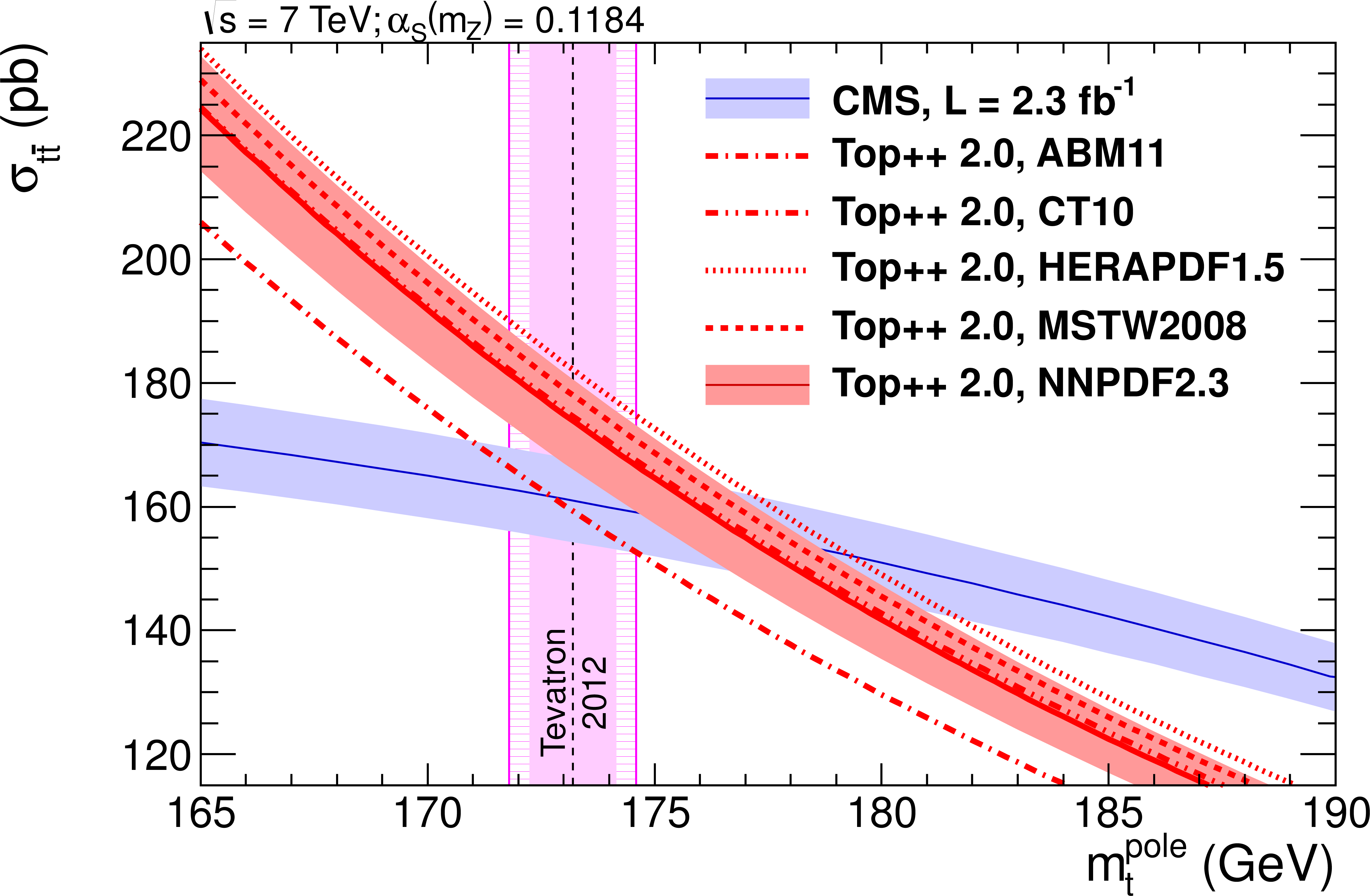
Figure 1-a:
Predicted $ {\mathrm {t}\overline {\mathrm {t}}}$ cross section at NNLO+NNLL, as a function of the top-quark pole mass (a) and of the strong coupling constant (b), using five different NNLO PDF sets, compared to the cross section measured by CMS assuming $ {m_ {\mathrm {t}}} = {m_ {\mathrm {t}}^{\scriptscriptstyle {\text {pole}}}} $. The uncertainties on the measured $\sigma _{ {\mathrm {t}\overline {\mathrm {t}}} }$ as well as the renormalization and factorization scale and PDF uncertainties on the prediction with NNPDF2.3 are illustrated with filled bands. The uncertainties on the $\sigma _{ {\mathrm {t}\overline {\mathrm {t}}} }$ predictions using the other PDF sets are indicated only in the right panel at the corresponding default $\alpha _S ( {m_ {\mathrm {Z}}} )$ values. The $ {m_ {\mathrm {t}}^{\scriptscriptstyle {\text {pole}}}} $ and $\alpha _S ( {m_ {\mathrm {Z}}} )$ regions favored by the direct measurements at the Tevatron and by the latest world average, respectively, are shown as hatched areas. In the left panel, the inner (solid) area of the vertical band corresponds to the original uncertainty of the direct $ {m_ {\mathrm {t}}} $ average, while the outer (hatched) area additionally accounts for the possible difference between this mass and $ {m_ {\mathrm {t}}^{\scriptscriptstyle {\text {pole}}}} $. |
png pdf |
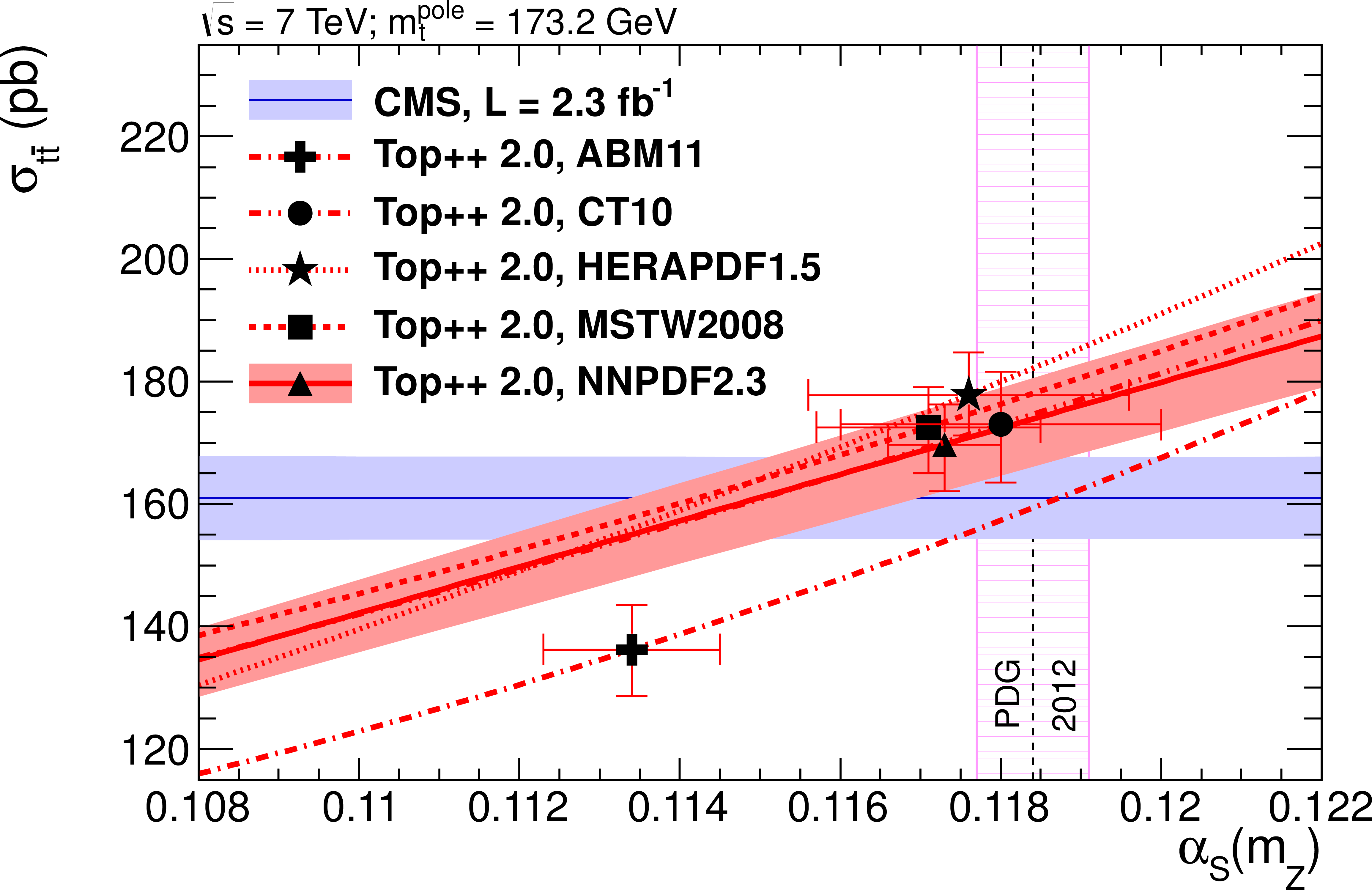
Figure 1-b:
Predicted $ {\mathrm {t}\overline {\mathrm {t}}}$ cross section at NNLO+NNLL, as a function of the top-quark pole mass (a) and of the strong coupling constant (b), using five different NNLO PDF sets, compared to the cross section measured by CMS assuming $ {m_ {\mathrm {t}}} = {m_ {\mathrm {t}}^{\scriptscriptstyle {\text {pole}}}} $. The uncertainties on the measured $\sigma _{ {\mathrm {t}\overline {\mathrm {t}}} }$ as well as the renormalization and factorization scale and PDF uncertainties on the prediction with NNPDF2.3 are illustrated with filled bands. The uncertainties on the $\sigma _{ {\mathrm {t}\overline {\mathrm {t}}} }$ predictions using the other PDF sets are indicated only in the right panel at the corresponding default $\alpha _S ( {m_ {\mathrm {Z}}} )$ values. The $ {m_ {\mathrm {t}}^{\scriptscriptstyle {\text {pole}}}} $ and $\alpha _S ( {m_ {\mathrm {Z}}} )$ regions favored by the direct measurements at the Tevatron and by the latest world average, respectively, are shown as hatched areas. In the left panel, the inner (solid) area of the vertical band corresponds to the original uncertainty of the direct $ {m_ {\mathrm {t}}} $ average, while the outer (hatched) area additionally accounts for the possible difference between this mass and $ {m_ {\mathrm {t}}^{\scriptscriptstyle {\text {pole}}}} $. |
png pdf |
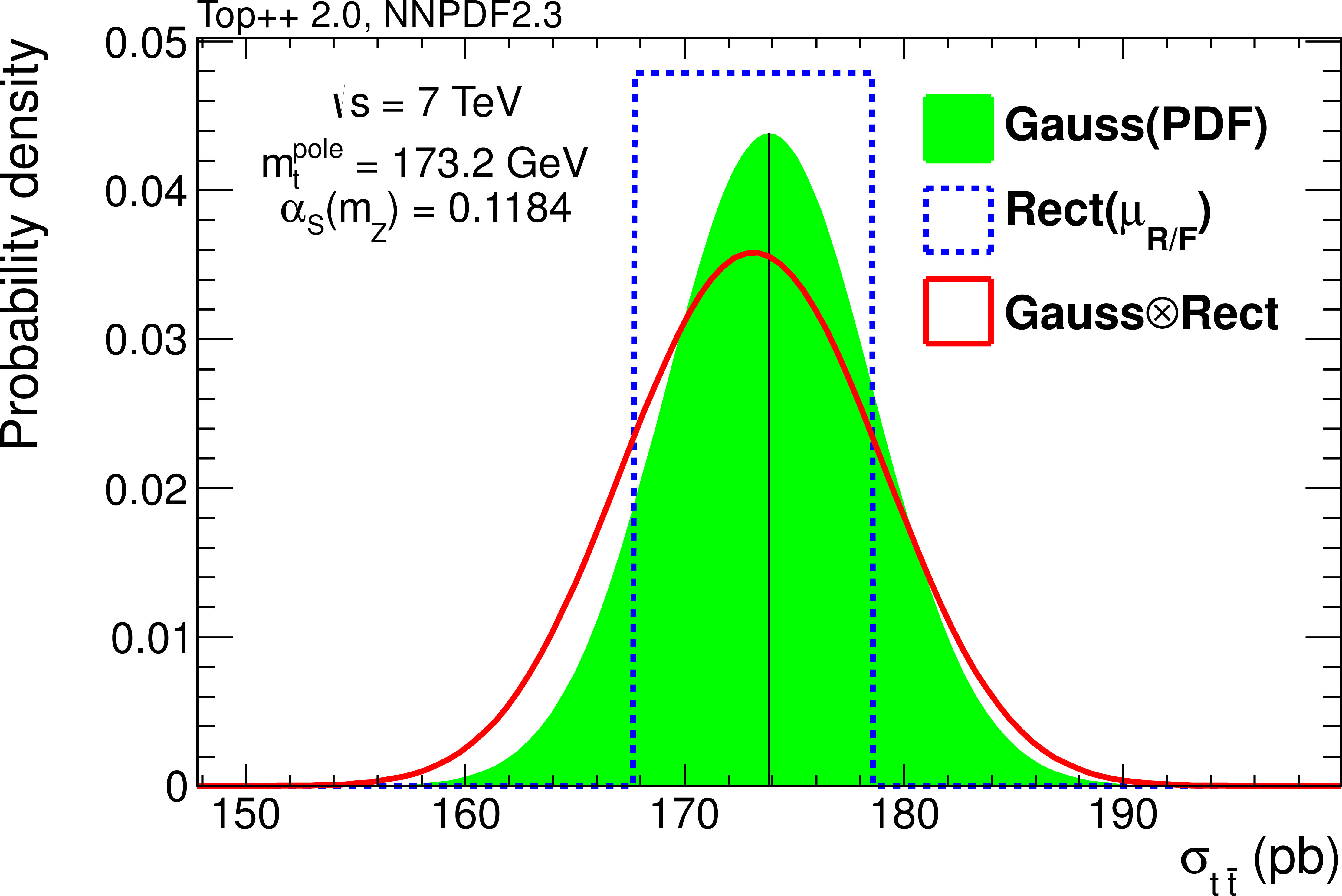
Figure 2:
Probability distributions for the predicted $ {\mathrm {t}\overline {\mathrm {t}}} $ cross section at NNLO+NNLL with $ {m_ {\mathrm {t}}^{\scriptscriptstyle {\text {pole}}}}$ = 173.2 GeV, $\alpha _S ( {m_ {\mathrm {Z}}} )$ = 0.1184 and the NNLO parton distributions from NNPDF2.3. The resulting probability, $f_{\text {th}} (\sigma _{ {\mathrm {t}\overline {\mathrm {t}}} })$, represented by a solid line, is obtained by convolving a Gaussian distribution (filled area) that accounts for the PDF uncertainty with a rectangular function (dashed line) that covers the scale variation uncertainty. |

png pdf |
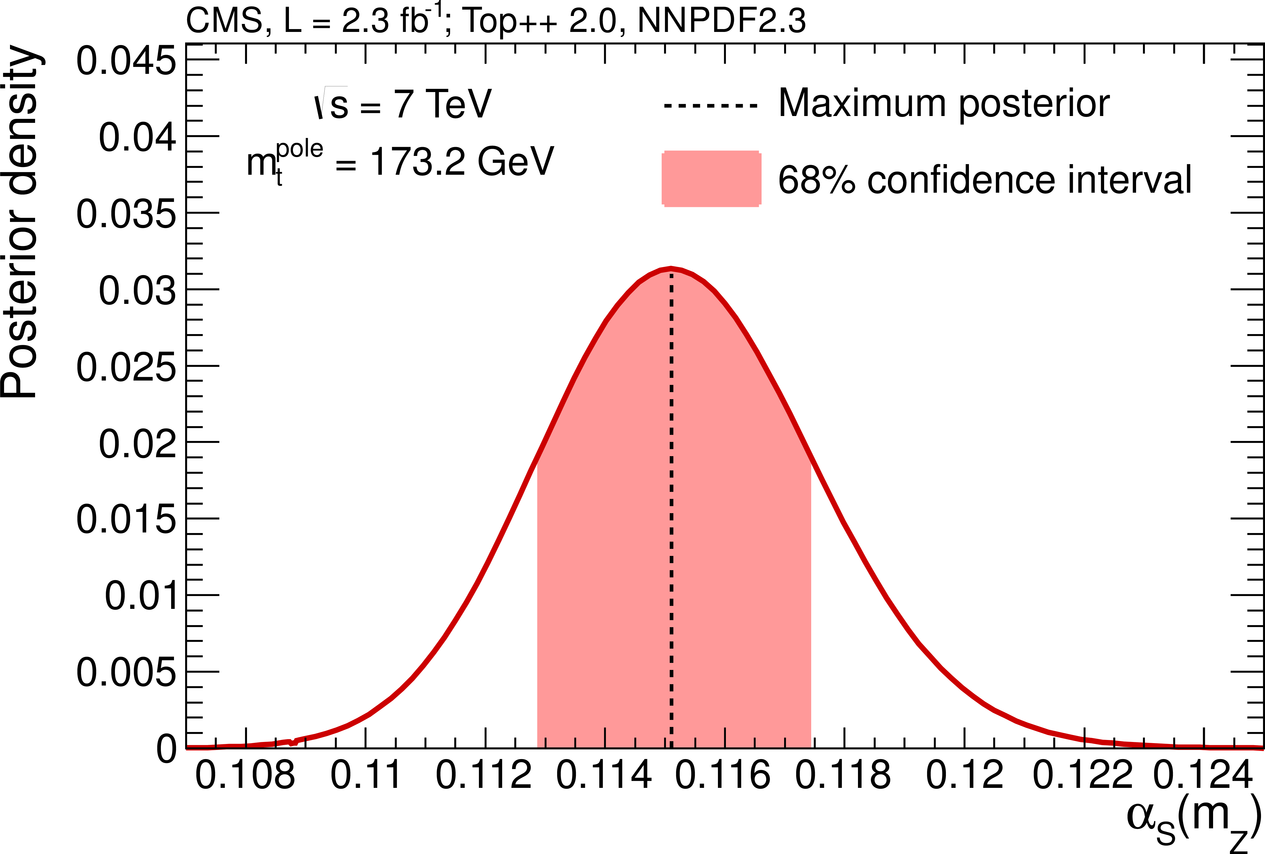
Figure 3-a:
Marginal posteriors $P ( {m_ {\mathrm {t}}^{\scriptscriptstyle {\text {pole}}}} )$ (a) and $P (\alpha _S)$ (b) based on the cross section prediction at NNLO+NNLL with the NNLO parton distributions from NNPDF2.3. The posteriors are constructed as described in the text. Here, $P ( {m_ {\mathrm {t}}^{\scriptscriptstyle {\text {pole}}}} )$ is shown for $\alpha _S ( {m_ {\mathrm {Z}}} )$ = 0.1184 and $P (\alpha _S)$ for $ {m_ {\mathrm {t}}^{\scriptscriptstyle {\text {pole}}}} $ = 173.2 GeV. |
png pdf |
Figure 3-b:
Marginal posteriors $P ( {m_ {\mathrm {t}}^{\scriptscriptstyle {\text {pole}}}} )$ (a) and $P (\alpha _S)$ (b) based on the cross section prediction at NNLO+NNLL with the NNLO parton distributions from NNPDF2.3. The posteriors are constructed as described in the text. Here, $P ( {m_ {\mathrm {t}}^{\scriptscriptstyle {\text {pole}}}} )$ is shown for $\alpha _S ( {m_ {\mathrm {Z}}} )$ = 0.1184 and $P (\alpha _S)$ for $ {m_ {\mathrm {t}}^{\scriptscriptstyle {\text {pole}}}} $ = 173.2 GeV. |
png pdf |
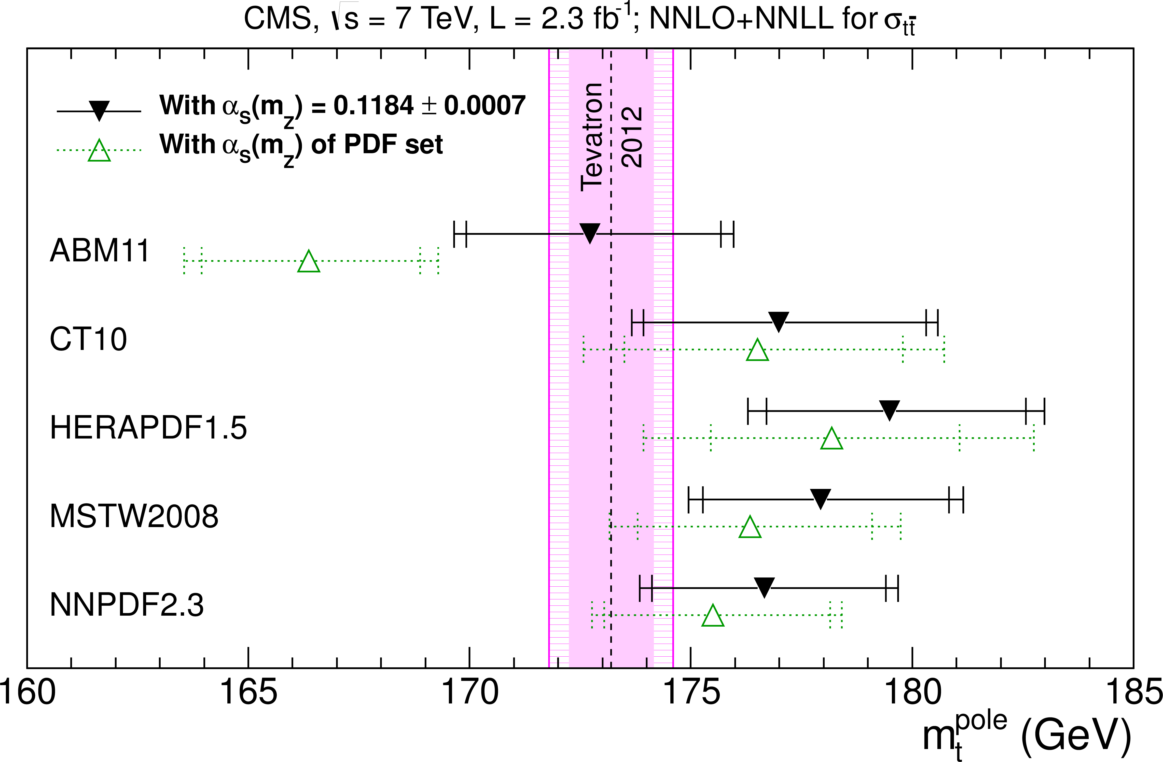
Figure 4:
Results obtained for $ {m_ {\mathrm {t}}^{\scriptscriptstyle {\text {pole}}}} $ from the measured $ {\mathrm {t}\overline {\mathrm {t}}} $ cross section together with the prediction at NNLO+NNLL using different NNLO PDF sets. The filled symbols represent the results obtained when using the $\alpha _S ( {m_ {\mathrm {Z}}} )$ world average, while the open symbols indicate the results obtained with the default $\alpha _S ( {m_ {\mathrm {Z}}} )$ value of the respective PDF set. The inner error bars include the uncertainties on the measured cross section and on the LHC beam energy as well as the PDF and scale uncertainties on the predicted cross section. The outer error bars additionally account for the uncertainty on the $\alpha _S ( {m_ {\mathrm {Z}}} )$ value used for a specific prediction. For comparison, the latest average of direct $ {m_ {\mathrm {t}}} $ measurements is shown as vertical band, where the inner (solid) area corresponds to the original uncertainty of the direct $ {m_ {\mathrm {t}}} $ average, while the outer (hatched) area additionally accounts for the possible difference between this mass and $ {m_ {\mathrm {t}}^{\scriptscriptstyle {\text {pole}}}} $. |

png pdf |
Figure 5:
Results obtained for $\alpha _S ( {m_ {\mathrm {Z}}} )$ from the measured $ {\mathrm {t}\overline {\mathrm {t}}}$ cross section together with the prediction at NNLO+NNLL using different NNLO PDF sets. The inner error bars include the uncertainties on the measured cross section and on the LHC beam energy as well as the PDF and scale uncertainties on the predicted cross section. The outer error bars additionally account for the uncertainty on $ {m_ {\mathrm {t}}^{\scriptscriptstyle {\text {pole}}}} $. For comparison, the latest $\alpha _S ( {m_ {\mathrm {Z}}} )$ world average with its uncertainty is shown as a hatched band. For each PDF set, the default $\alpha _S ( {m_ {\mathrm {Z}}} )$ value and its uncertainty are indicated using a dotted line and a shaded band. |
|
|
Compact Muon Solenoid LHC, CERN |
|

|

|

|

|

|