

Compact Muon Solenoid
LHC, CERN
| CMS-TOP-14-022 ; CERN-PH-EP/2015-234 | ||
| Measurement of the top quark mass using proton-proton data at $\sqrt{s} =$ 7 and 8 TeV | ||
| CMS Collaboration | ||
| 15 September 2015 | ||
| Phys. Rev. D 93 (2016) 072004 | ||
| Abstract: A new set of measurements of the top quark mass are presented, based on the proton-proton data recorded by the CMS experiment at the LHC at $\sqrt{s} =$ 8 TeV corresponding to a luminosity of 19.7 fb$^{-1}$. The top quark mass is measured using the lepton+jets, all-jets and dilepton decay channels, giving values of 172.35 $\pm$ 0.16 (stat) $\pm$ 0.48 (syst) GeV, 172.32 $\pm$ 0.25 (stat) $\pm$ 0.59 (syst) GeV, and 172.82 $\pm$ 0.19 (stat) $\pm$ 1.22 (syst) GeV, respectively. When combined with the published CMS results at $\sqrt{s} =$ 7 TeV, they provide a top quark mass measurement of 172.44 $\pm$ 0.13 (stat) $\pm$ 0.47 (syst) GeV. The top quark mass is also studied as a function of the event kinematical properties in the lepton+jets decay channel. No indications of a kinematic bias are observed and the collision data are consistent with a range of predictions from current theoretical models of $ \mathrm{ t \bar{t} } $ production. | ||
| Links: e-print arXiv:1509.04044 [hep-ex] (PDF) ; CDS record ; inSPIRE record ; HepData record ; CADI line (restricted) ; | ||
| Figures | |
png pdf |
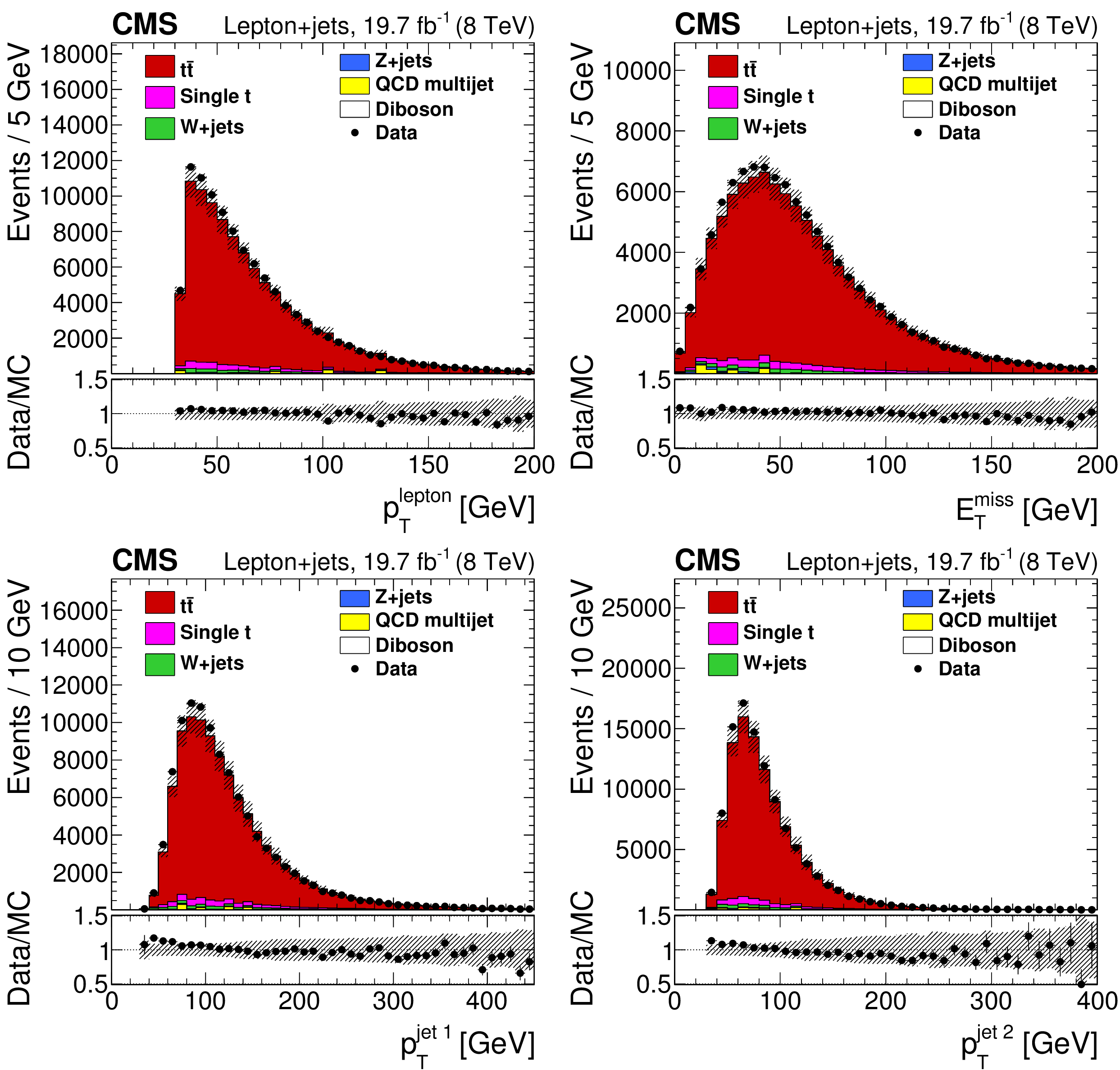
Figure 1:
Distributions for the lepton+jets channel of (top left) lepton $ {p_{\mathrm {T}}} $, (top right) missing transverse energy, (bottom left) leading jet $ {p_{\mathrm {T}}} $, (bottom right) second-leading jet $ {p_{\mathrm {T}}} $ for data and simulation, summed over all channels and normalized by luminosity. The vertical bars show the statistical uncertainty and the hatched bands show the statistical and systematic uncertainties added in quadrature. The lower portion of each panel shows the ratio of the yields between the collision data and the simulation. |
png pdf |
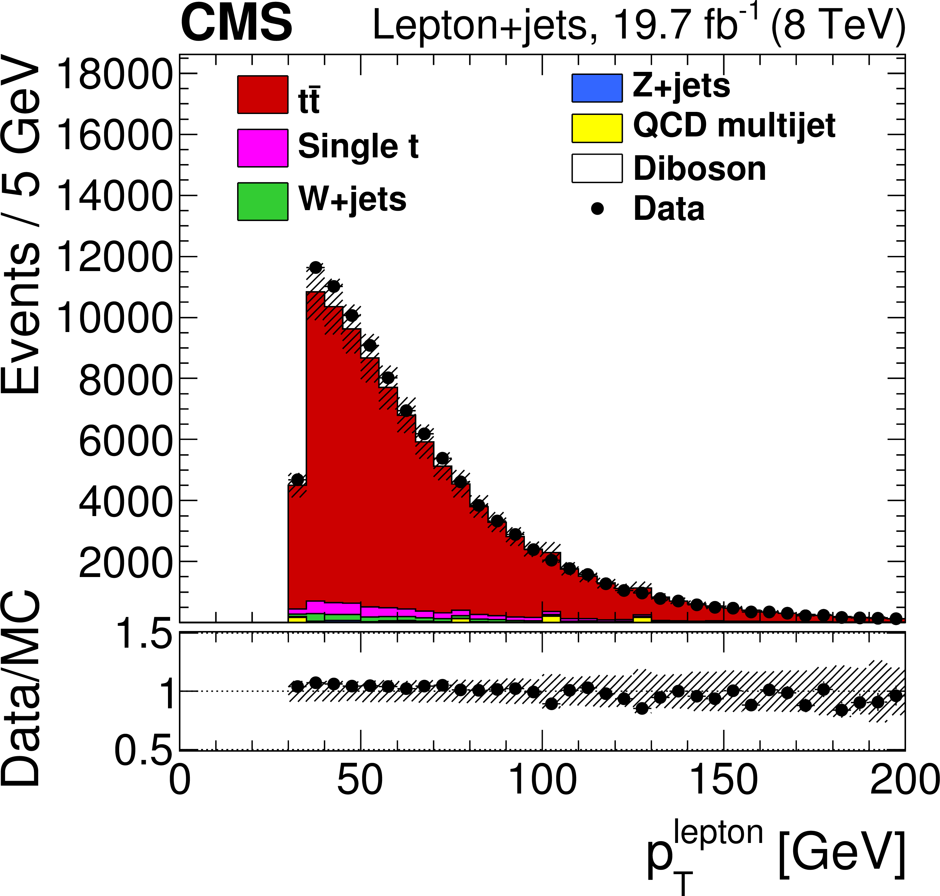
Figure 1-a:
Distribution for the lepton+jets channel of lepton $ {p_{\mathrm {T}}} $ for data and simulation, summed over all channels and normalized by luminosity. The vertical bars show the statistical uncertainty and the hatched bands show the statistical and systematic uncertainties added in quadrature. The lower portion of each panel shows the ratio of the yields between the collision data and the simulation. |

png pdf |
Figure 1-b:
Distribution for the lepton+jets channel of missing transverse energy for data and simulation, summed over all channels and normalized by luminosity. The vertical bars show the statistical uncertainty and the hatched bands show the statistical and systematic uncertainties added in quadrature. The lower portion of each panel shows the ratio of the yields between the collision data and the simulation. |
png pdf |
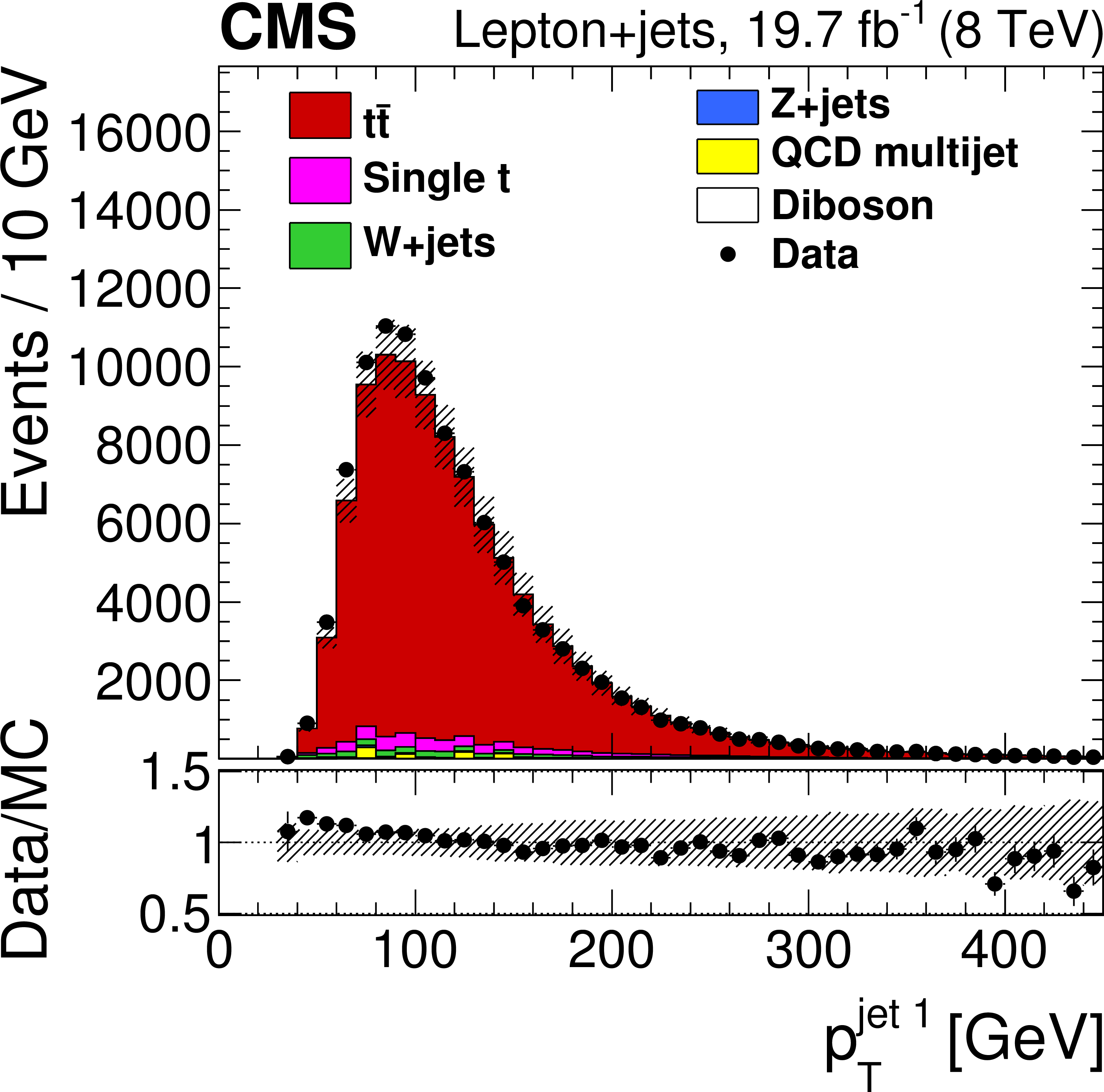
Figure 1-c:
Distribution for the lepton+jets channel of leading jet $ {p_{\mathrm {T}}} $ for data and simulation, summed over all channels and normalized by luminosity. The vertical bars show the statistical uncertainty and the hatched bands show the statistical and systematic uncertainties added in quadrature. The lower portion of each panel shows the ratio of the yields between the collision data and the simulation. |
png pdf |
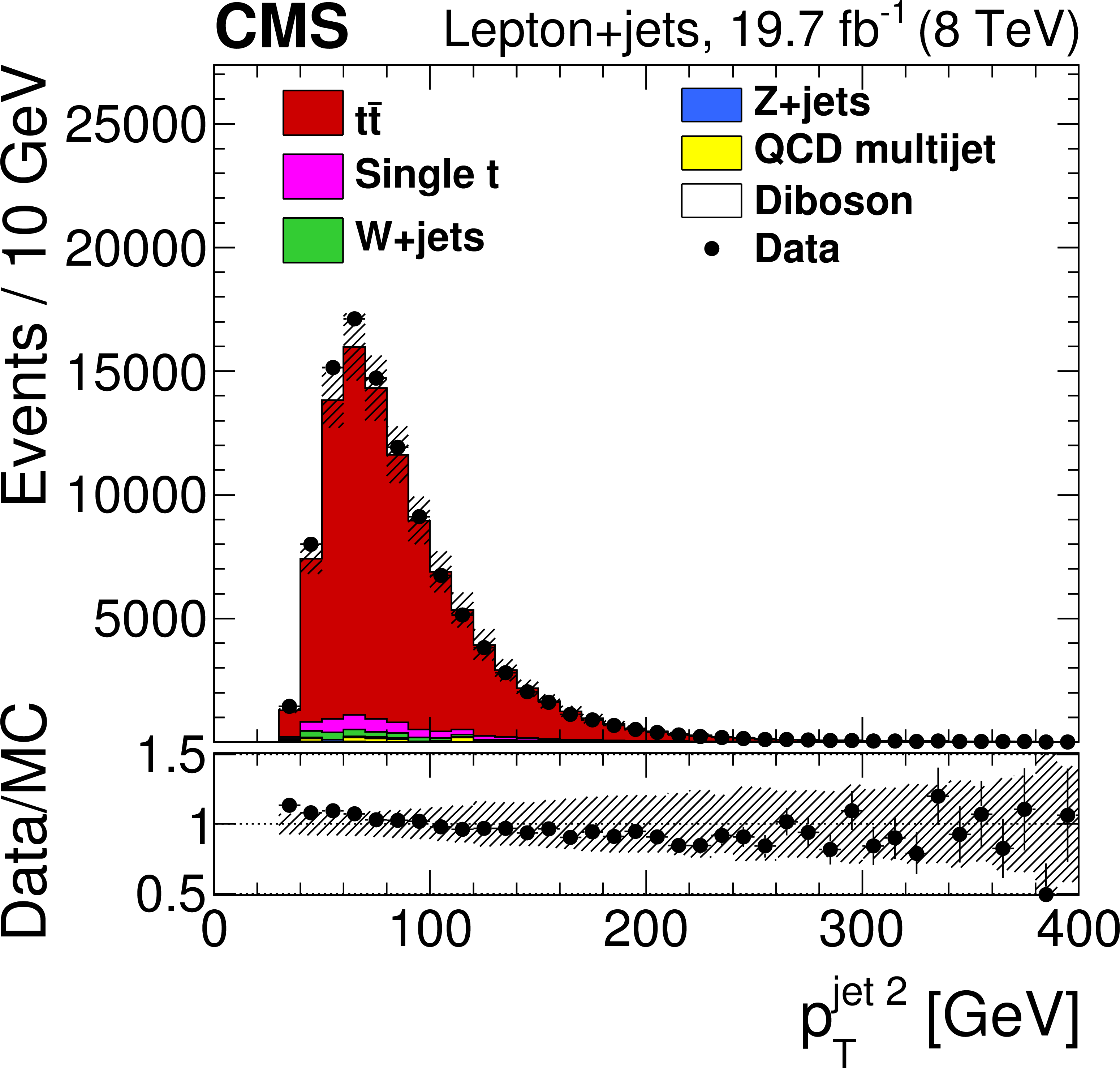
Figure 1-d:
Distribution for the lepton+jets channel of second-leading jet $ {p_{\mathrm {T}}} $ for data and simulation, summed over all channels and normalized by luminosity. The vertical bars show the statistical uncertainty and the hatched bands show the statistical and systematic uncertainties added in quadrature. The lower portion of each panel shows the ratio of the yields between the collision data and the simulation. |

png pdf |
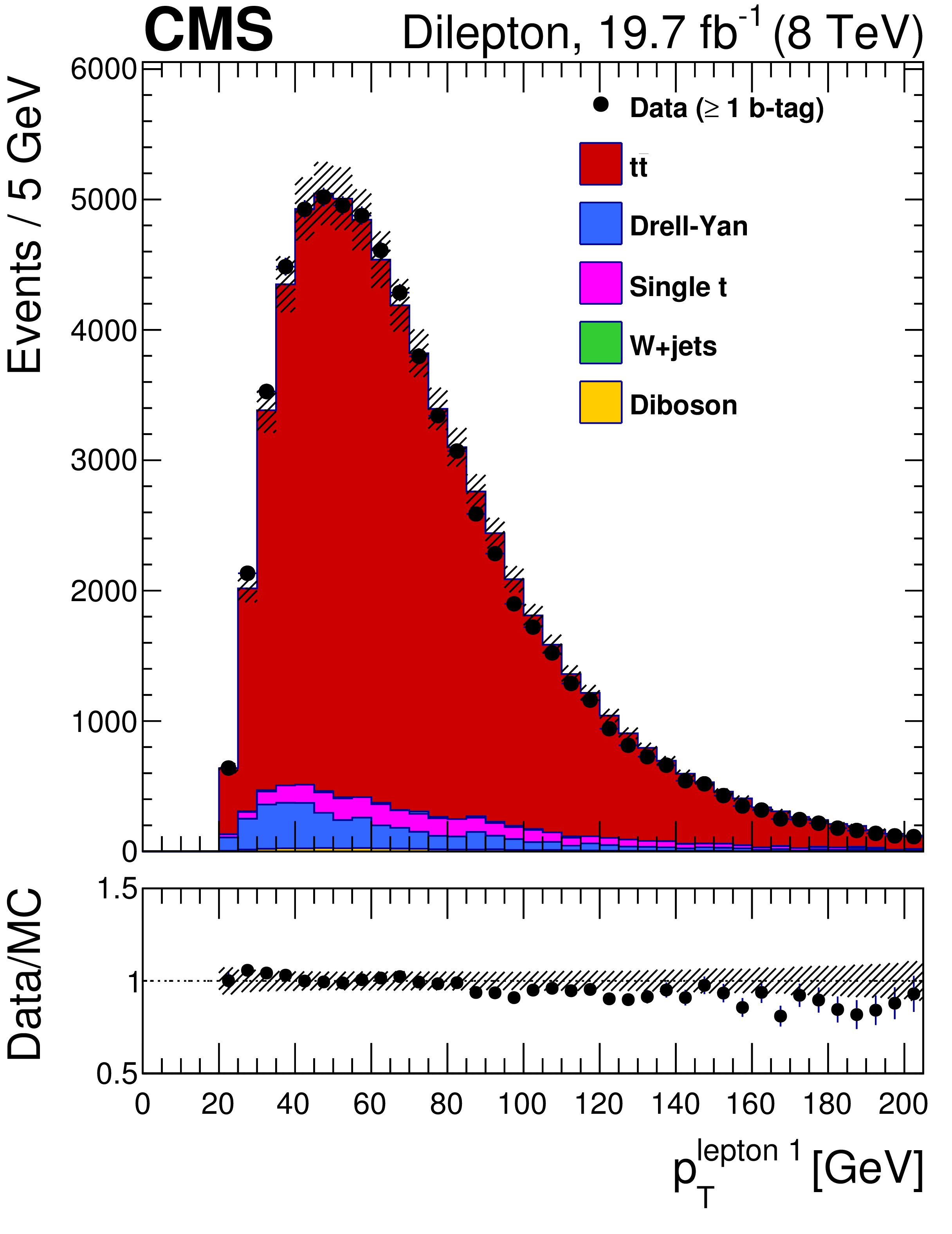
Figure 2:
Distributions for the dilepton channel: (top left) leading lepton $ {p_{\mathrm {T}}} $, (top right) second-leading lepton $ {p_{\mathrm {T}}} $, (bottom left) leading jet $ {p_{\mathrm {T}}} $, (bottom right) second-leading jet $ {p_{\mathrm {T}}} $ for data and simulation, summed over all channels and normalized by luminosity. The vertical bars show the statistical uncertainty and the hatched bands show the statistical and systematic uncertainties added in quadrature. The lower portion of each panel shows the ratio of the yields between the collision data and the simulation. |
png pdf |
Figure 2-a:
Dilepton channel: leading lepton $ {p_{\mathrm {T}}} $ for data and simulation, summed over all channels and normalized by luminosity. The vertical bars show the statistical uncertainty and the hatched bands show the statistical and systematic uncertainties added in quadrature. The lower portion of each panel shows the ratio of the yields between the collision data and the simulation. |

png pdf |
Figure 2-b:
Dilepton channel: second-leading lepton $ {p_{\mathrm {T}}} $ for data and simulation, summed over all channels and normalized by luminosity. The vertical bars show the statistical uncertainty and the hatched bands show the statistical and systematic uncertainties added in quadrature. The lower portion of each panel shows the ratio of the yields between the collision data and the simulation. |

png pdf |
Figure 2-c:
Dilepton channel: leading jet $ {p_{\mathrm {T}}} $ for data and simulation, summed over all channels and normalized by luminosity. The vertical bars show the statistical uncertainty and the hatched bands show the statistical and systematic uncertainties added in quadrature. The lower portion of each panel shows the ratio of the yields between the collision data and the simulation. |

png pdf |
Figure 2-d:
Dilepton channel: second-leading jet $ {p_{\mathrm {T}}} $ for data and simulation, summed over all channels and normalized by luminosity. The vertical bars show the statistical uncertainty and the hatched bands show the statistical and systematic uncertainties added in quadrature. The lower portion of each panel shows the ratio of the yields between the collision data and the simulation. |
png pdf |
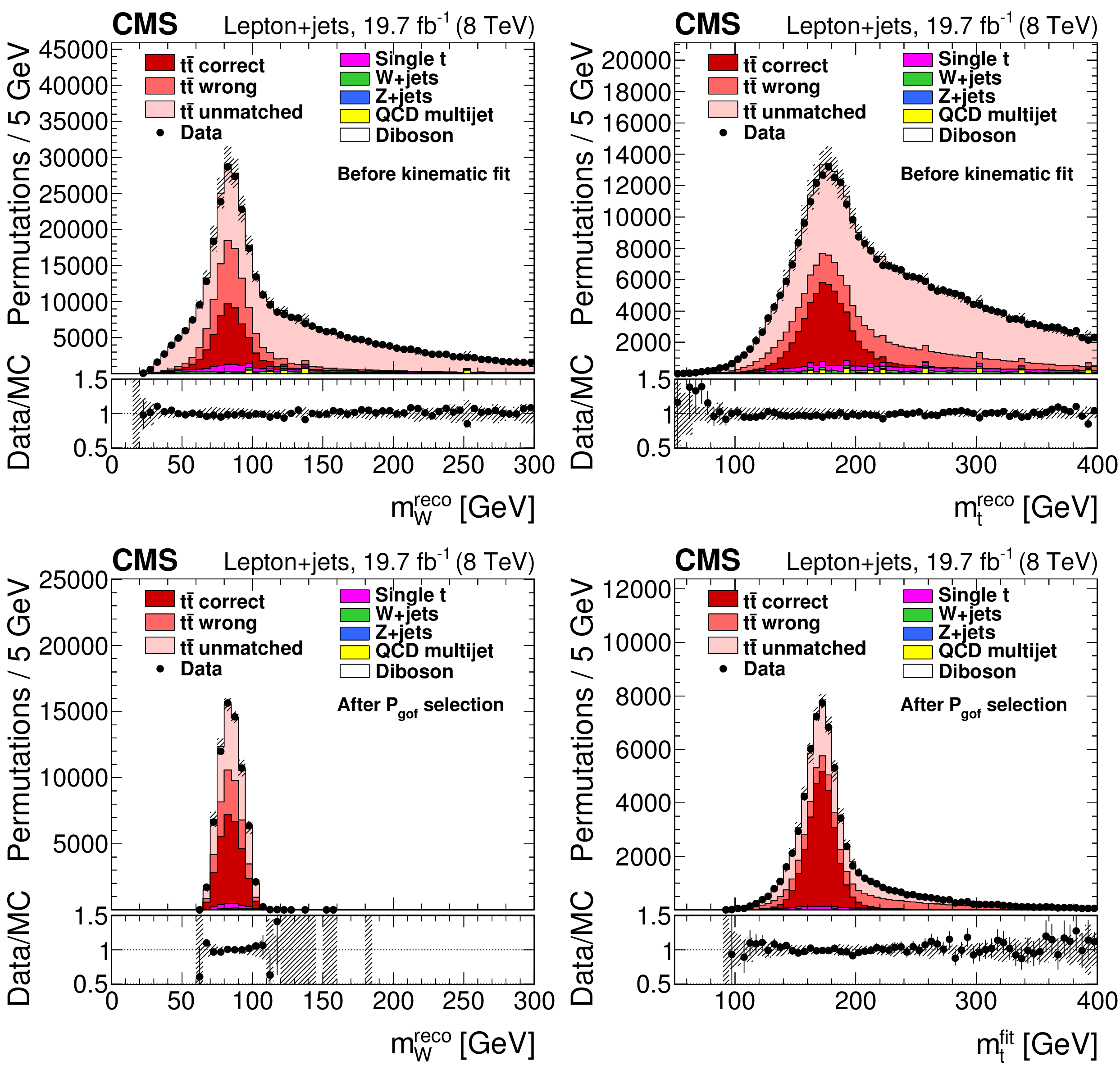
Figure 3:
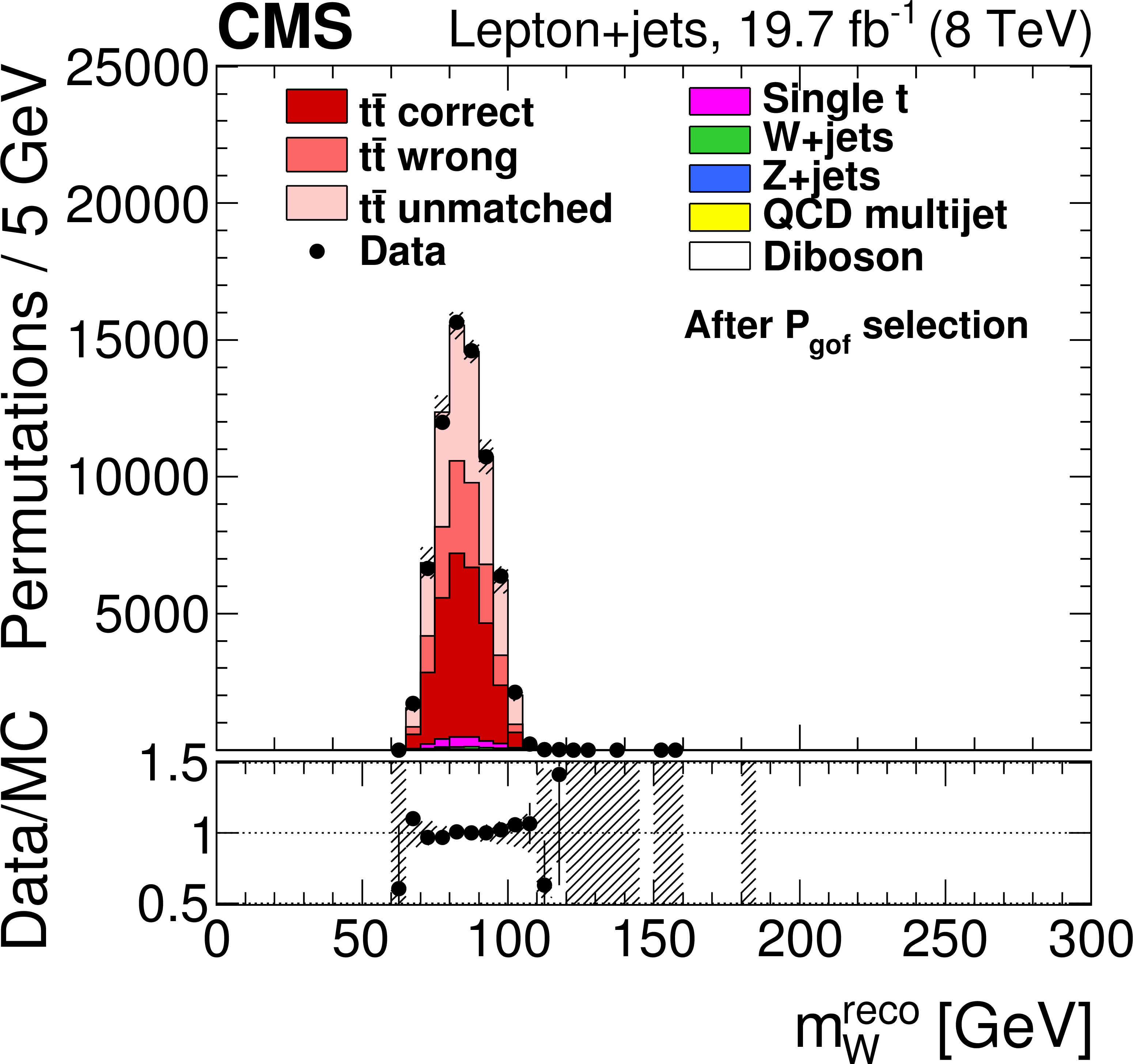
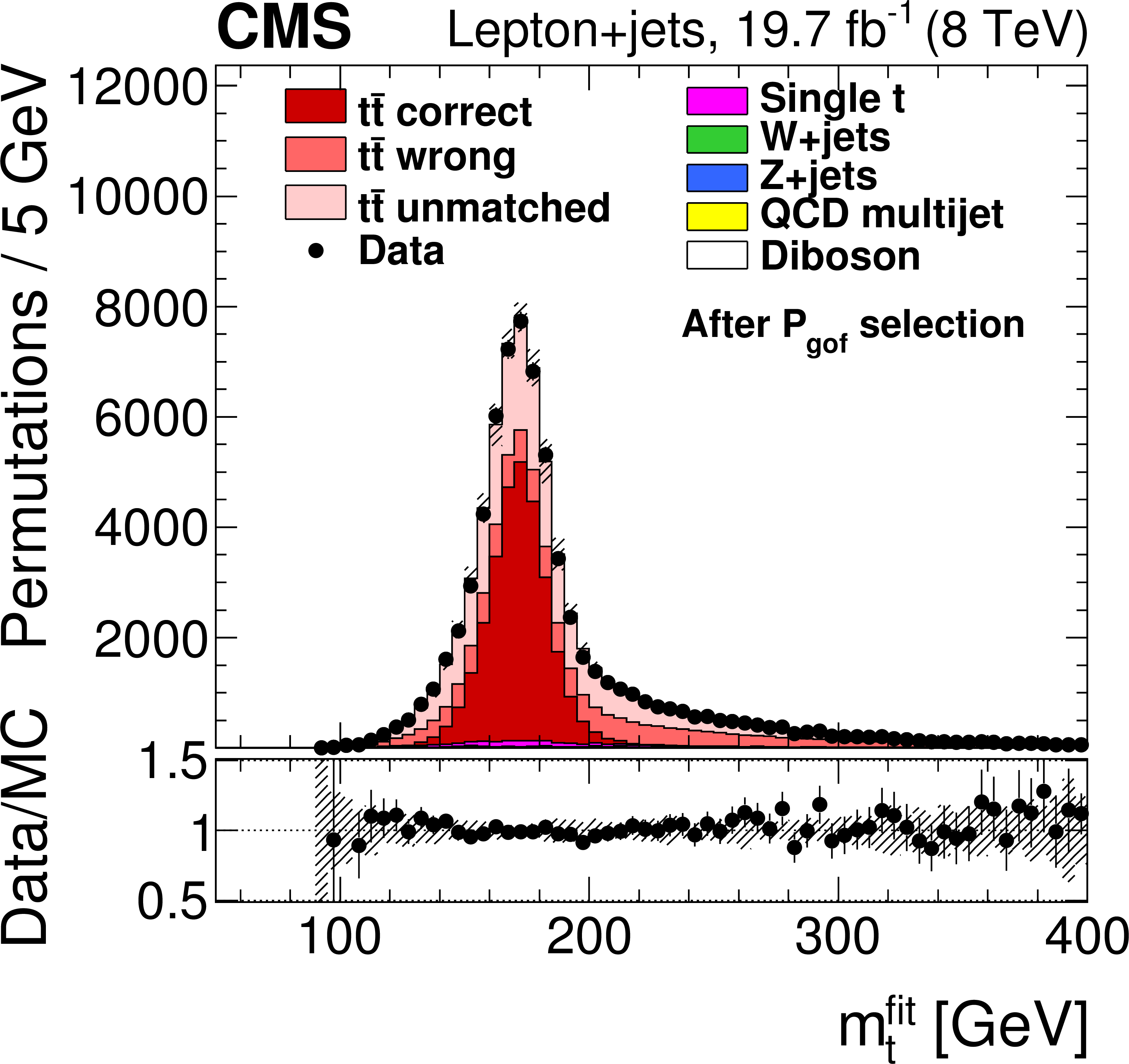
Reconstructed masses of (top left) the W bosons decaying to $ {\mathrm {q}} {\overline {\mathrm {q}}} $ pairs and (top right) the corresponding top quarks, prior to the kinematic fitting to the $ {\mathrm {t}\overline {\mathrm {t}}} $ hypothesis. Panels (bottom left) and (bottom right) show, respectively, the reconstructed W boson masses and the fitted top quark masses after the goodness-of-fit selection and the weighting by $P_{\mathrm {gof} }$. The total number of permutations found in simulation is normalized to be the same as the total number of permutations observed in data. The vertical bars show the statistical uncertainty and the hatched bands show the statistical and systematic uncertainties added in quadrature. The lower portion of each panel shown the ratio of the yields between the collision data and the simulation. |
png pdf |
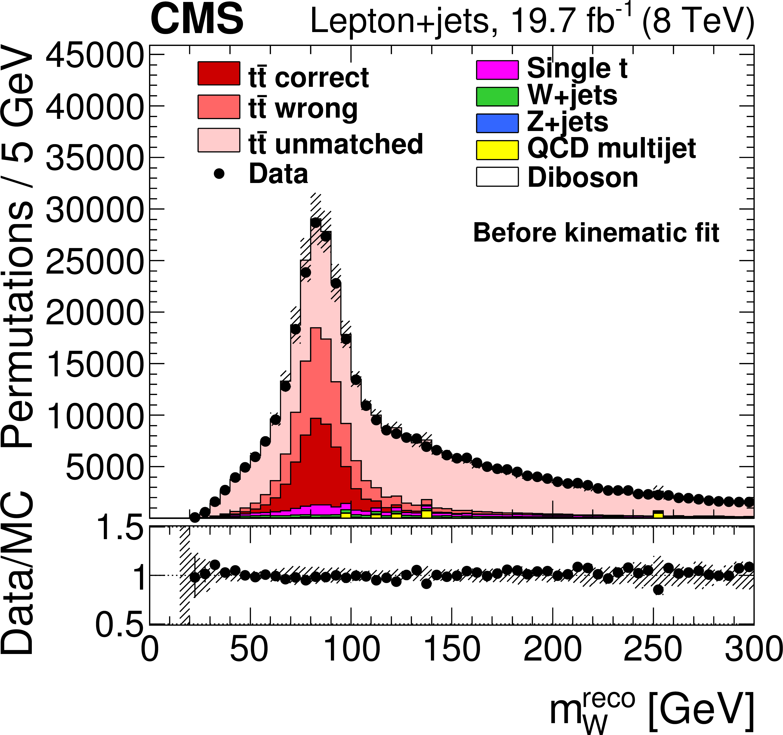
Figure 3-a:
Reconstructed mass of the W bosons decaying to $ {\mathrm {q}} {\overline {\mathrm {q}}} $ pairs, prior to the kinematic fitting to the $ {\mathrm {t}\overline {\mathrm {t}}} $ hypothesis. The total number of permutations found in simulation is normalized to be the same as the total number of permutations observed in data. The vertical bars show the statistical uncertainty and the hatched bands show the statistical and systematic uncertainties added in quadrature. The lower portion of the panel shows the ratio of the yields between the collision data and the simulation. |
png pdf |
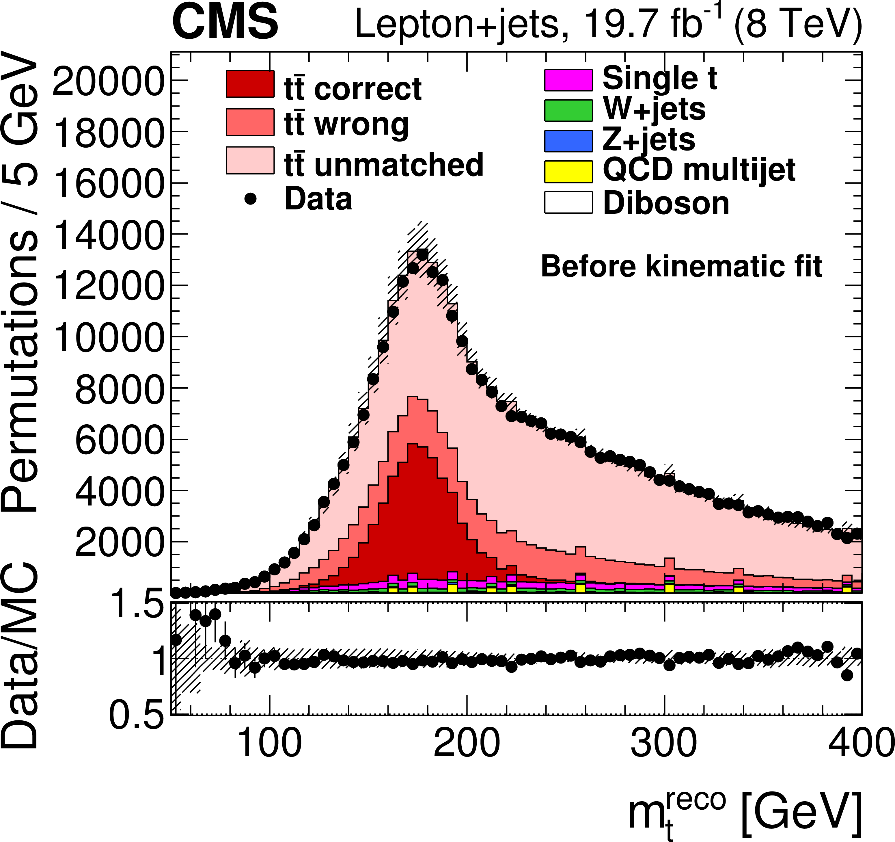
Figure 3-b:
Reconstructed mass of the top quarks corresponding to the W bosons decaying to $ {\mathrm {q}} {\overline {\mathrm {q}}} $ pairs, prior to the kinematic fitting to the $ {\mathrm {t}\overline {\mathrm {t}}} $ hypothesis. The total number of permutations found in simulation is normalized to be the same as the total number of permutations observed in data. The vertical bars show the statistical uncertainty and the hatched bands show the statistical and systematic uncertainties added in quadrature. The lower portion of the panel shows the ratio of the yields between the collision data and the simulation. |
png pdf |
Figure 3-c:
Reconstructed W boson masses after the goodness-of-fit selection and the weighting by $P_{\mathrm {gof} }$. The total number of permutations found in simulation is normalized to be the same as the total number of permutations observed in data. The vertical bars show the statistical uncertainty and the hatched bands show the statistical and systematic uncertainties added in quadrature. The lower portion of the panel shows the ratio of the yields between the collision data and the simulation. |
png pdf |
Figure 3-d:
Fitted top quark masses after the goodness-of-fit selection and the weighting by $P_{\mathrm {gof} }$. The total number of permutations found in simulation is normalized to be the same as the total number of permutations observed in data. The vertical bars show the statistical uncertainty and the hatched bands show the statistical and systematic uncertainties added in quadrature. The lower portion of the panel shows the ratio of the yields between the collision data and the simulation. |

png pdf |
Figure 4:
The two-dimensional likelihood ($-2 \Delta \log\left (\mathcal {L}\right )$) for the lepton+jets channel for the 2D, hybrid, and 1D fits. The thick (thin) ellipses correspond to contours of $-2 \Delta \log\left (\mathcal {L}\right ) =$ 1 (4) allowing the construction of the one (two) $\sigma $ statistical intervals of $ {m_{ {\mathrm {t}} }} $. For the 1D fit, the thick and thin lines correspond to the one and two $\sigma $ statistical uncertainties, respectively. |
png pdf |
Figure 5:
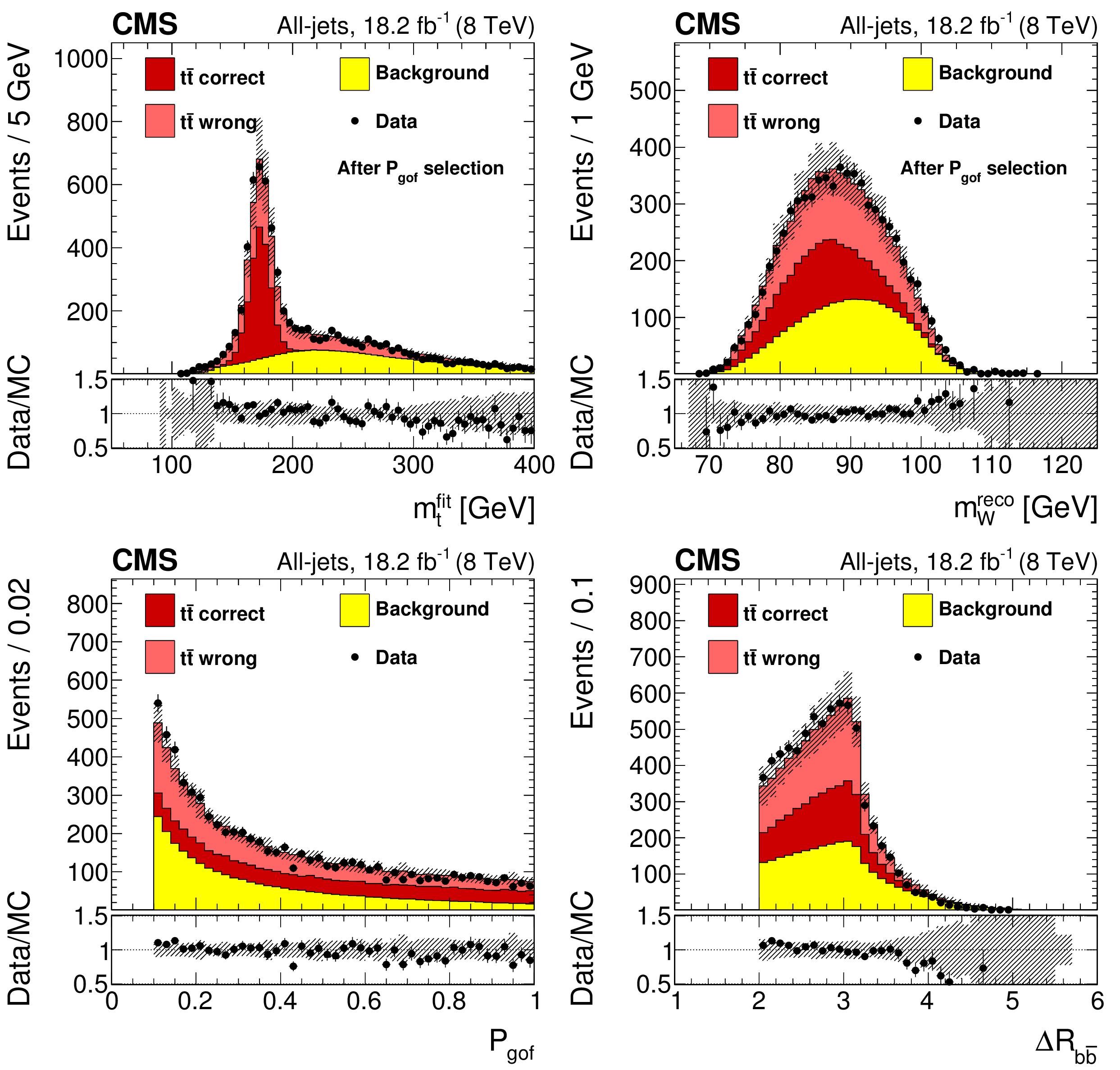
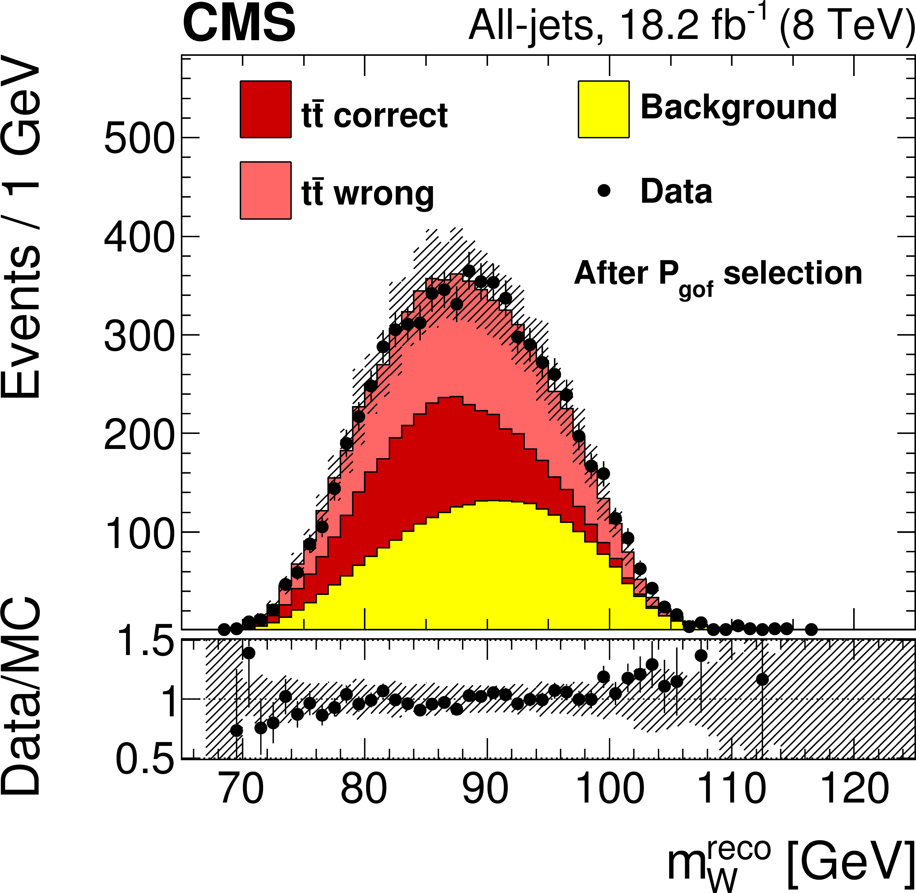
Distributions of (top left) the reconstructed top quark mass from the kinematic fit, (top right) the average reconstructed W boson mass, (bottom left) the goodness-of-fit probability, and (bottom right) the separation of the two b quark jets for the all-jets channel. The simulated $ {\mathrm {t}\overline {\mathrm {t}}} $ signal and the background from the control sample are normalized to data. The value of $ {m_{ {\mathrm {t}} }} $ used in the simulation is 172.5 GeV and the nominal jet energy scale is applied. The vertical bars show the statistical uncertainty and the hatched bands show the statistical and systematic uncertainties added in quadrature. The lower portion of each panel shows the ratio of the yields between the collision data and the simulation. |

png pdf |
Figure 5-a:
Distribution of the reconstructed top quark mass from the kinematic fit for the all-jets channel. The simulated $ {\mathrm {t}\overline {\mathrm {t}}} $ signal and the background from the control sample are normalized to data. The value of $ {m_{ {\mathrm {t}} }} $ used in the simulation is 172.5 GeV and the nominal jet energy scale is applied. The vertical bars show the statistical uncertainty and the hatched bands show the statistical and systematic uncertainties added in quadrature. The lower portion of each panel shows the ratio of the yields between the collision data and the simulation. |
png pdf |
Figure 5-b:
Distribution of the average reconstructed W boson mass for the all-jets channel. The simulated $ {\mathrm {t}\overline {\mathrm {t}}} $ signal and the background from the control sample are normalized to data. The value of $ {m_{ {\mathrm {t}} }} $ used in the simulation is 172.5 GeV and the nominal jet energy scale is applied. The vertical bars show the statistical uncertainty and the hatched bands show the statistical and systematic uncertainties added in quadrature. The lower portion of each panel shows the ratio of the yields between the collision data and the simulation. |
png pdf |
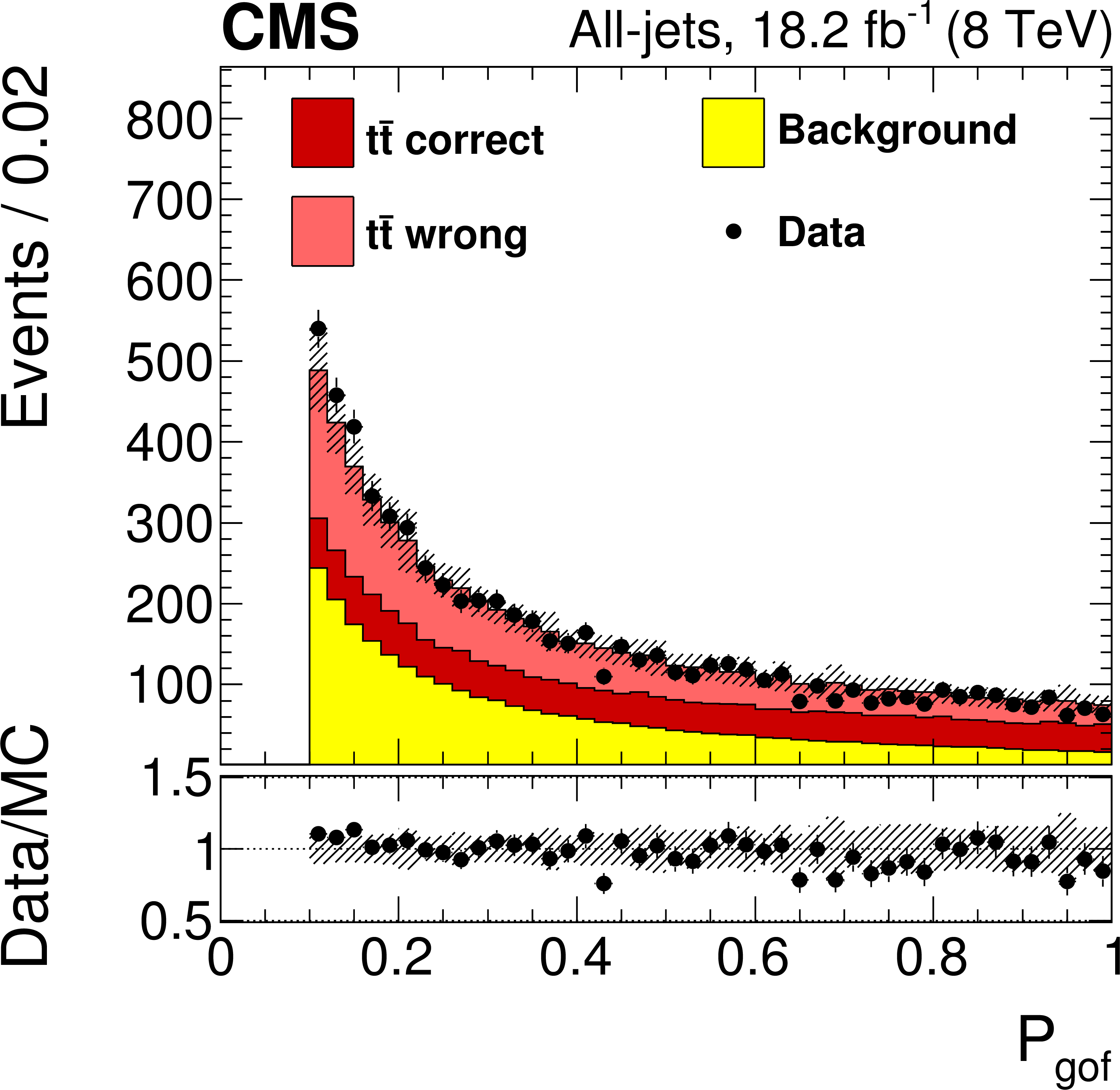
Figure 5-c:
Distribution of the goodness-of-fit probability for the all-jets channel. The simulated $ {\mathrm {t}\overline {\mathrm {t}}} $ signal and the background from the control sample are normalized to data. The value of $ {m_{ {\mathrm {t}} }} $ used in the simulation is 172.5 GeV and the nominal jet energy scale is applied. The vertical bars show the statistical uncertainty and the hatched bands show the statistical and systematic uncertainties added in quadrature. The lower portion of each panel shows the ratio of the yields between the collision data and the simulation. |

png pdf |
Figure 5-d:
Distribution of the separation of the two b quark jets for the all-jets channel. The simulated $ {\mathrm {t}\overline {\mathrm {t}}} $ signal and the background from the control sample are normalized to data. The value of $ {m_{ {\mathrm {t}} }} $ used in the simulation is 172.5 GeV and the nominal jet energy scale is applied. The vertical bars show the statistical uncertainty and the hatched bands show the statistical and systematic uncertainties added in quadrature. The lower portion of each panel shows the ratio of the yields between the collision data and the simulation. |
png pdf |
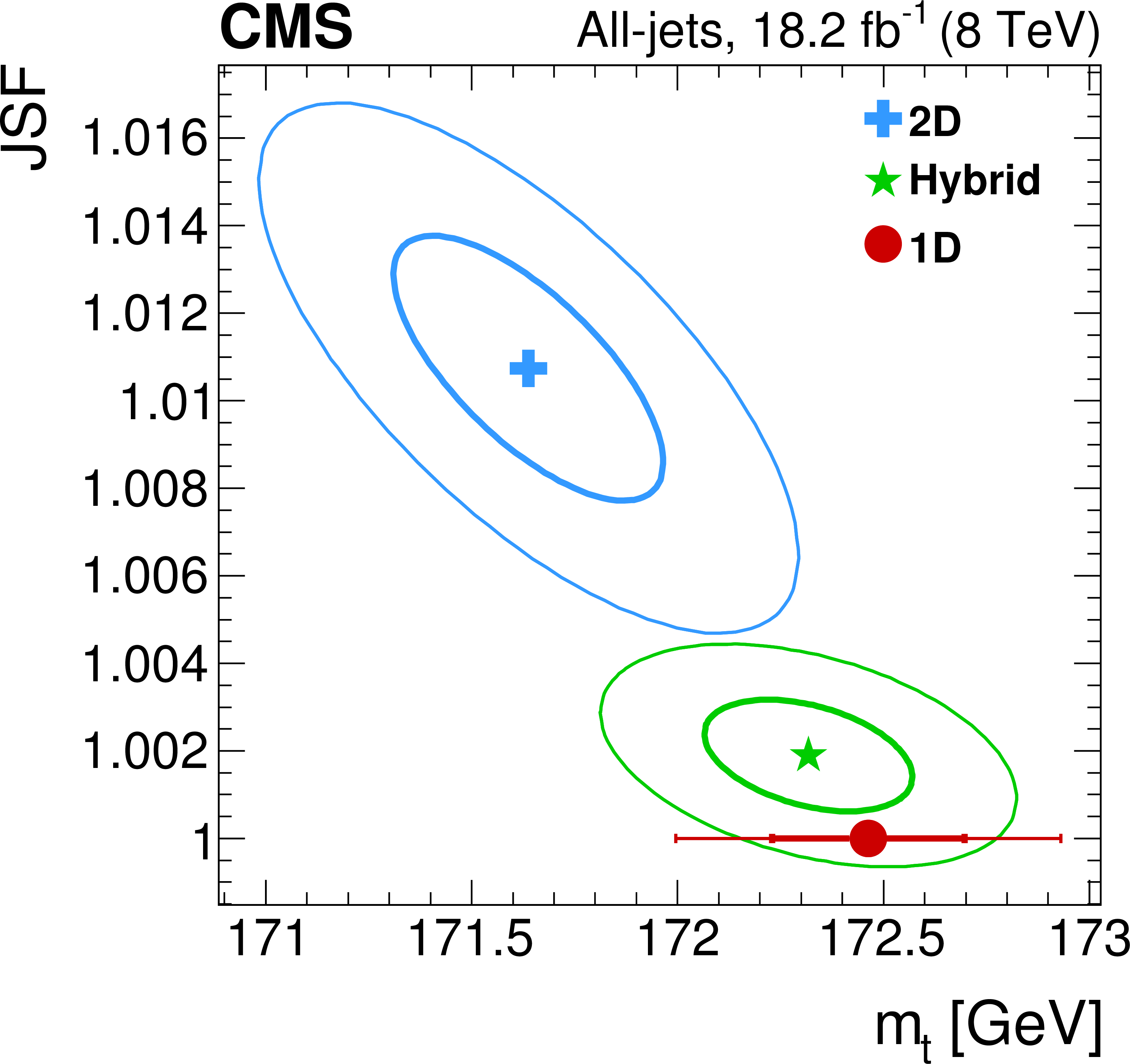
Figure 6:
The two-dimensional likelihood ($-2 \Delta \log\left (\mathcal {L}\right )$) for the all-jets channel for the 2D, hybrid, and 1D fits. The thick (thin) ellipses correspond to contours of $-2 \Delta \log\left (\mathcal {L}\right ) =$ 1 (4) allowing the construction of the one (two) $\sigma $ statistical intervals of $ {m_{ {\mathrm {t}} }} $. For the 1D fit, the thick and thin lines correspond to the one and two $\sigma $ statistical uncertainties, respectively. |
png pdf |
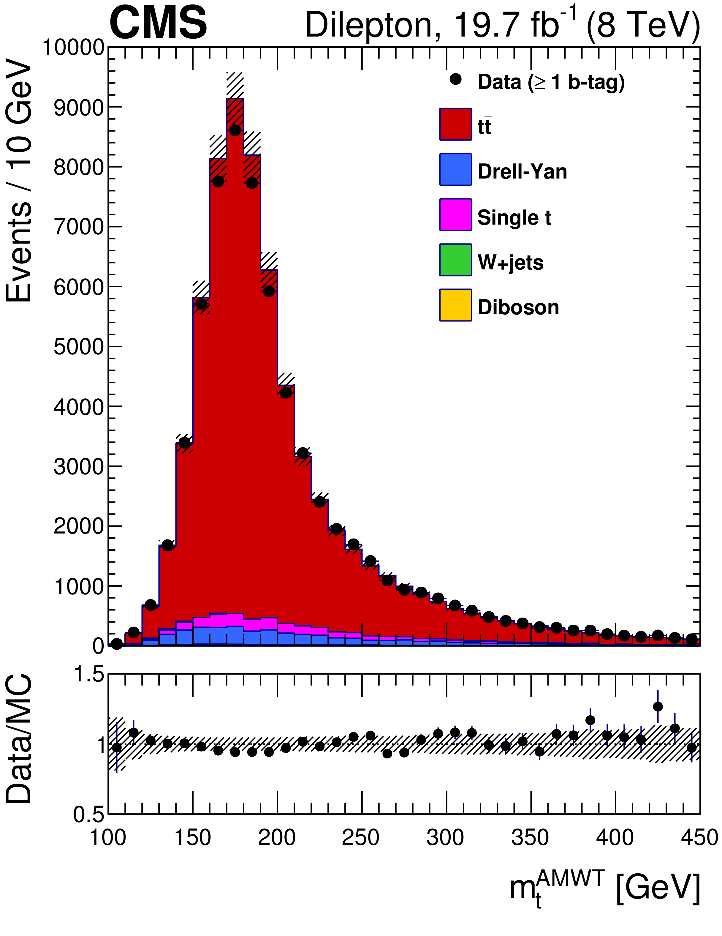
Figure 7:
Distribution of $m_{ {\mathrm {t}} }^{\mathrm {AMWT}}$ for the collision and simulated data with $ {m_{ {\mathrm {t}} }} =$ 172.5 GeV. The vertical bars show the statistical uncertainty and the hatched bands show the statistical and systematic uncertainties added in quadrature. The lower section of the plot shows the ratio of the yields between the collision data and the simulation. |

png pdf |
Figure 8:
Plot of the negative log-likelihood for data for the dilepton analysis. The continuous line represents a parabolic fit to the points. |

png pdf |
Figure 9:
Measurements of $ {m_{ {\mathrm {t}} }} $ as a function of the transverse momentum of the hadronically decaying top quark ($ {p_{\mathrm {T}}} ^{\rm {t,had}}$), the invariant mass of the $ {\mathrm {t}\overline {\mathrm {t}}} $ system ($m_{ {\mathrm {t}\overline {\mathrm {t}}} }$), the transverse momentum of the $ {\mathrm {t}\overline {\mathrm {t}}} $ system ($ {p_{\mathrm {T}}} ^{ {\mathrm {t}\overline {\mathrm {t}}} }$), and the number of jets with $ {p_{\mathrm {T}}} >$ 30 GeV. The filled circles represent the data, and the other symbols are for the simulations. For reasons of clarity the horizontal error bars are shown only for the data points and each of the simulations is shown as a single offset point with a vertical error bar representing its statistical uncertainty. The statistical uncertainty of the data is displayed by the inner error bars. For the outer error bars, the systematic uncertainties are added in quadrature. The open circles correspond to MadGraph with the PYTHIA Z2* tune, the open squares to MadGraph with the PYTHIA Perugia 2011 tune, and the open triangles represent MadGraph with the PYTHIA Perugia 2011 noCR tune. The open diamonds correspond to POWHEG with the PYTHIA Z2* tune and the open crosses correspond to POWHEG with HERWIG 6. The filled stars are for MC@NLO with HERWIG 6 and the open stars are for SHERPA. |

png pdf |
Figure 9-a:
Measurement of $ {m_{ {\mathrm {t}} }} $ as a function of the transverse momentum of the hadronically decaying top quark ($ {p_{\mathrm {T}}} ^{\rm {t,had}}$). The filled circles represent the data, and the other symbols are for the simulations. For reasons of clarity the horizontal error bars are shown only for the data points and each of the simulations is shown as a single offset point with a vertical error bar representing its statistical uncertainty. The statistical uncertainty of the data is displayed by the inner error bars. For the outer error bars, the systematic uncertainties are added in quadrature. The open circles correspond to MadGraph with the PYTHIA Z2* tune, the open squares to MadGraph with the PYTHIA Perugia 2011 tune, and the open triangles represent MadGraph with the PYTHIA Perugia 2011 noCR tune. The open diamonds correspond to POWHEG with the PYTHIA Z2* tune and the open crosses correspond to POWHEG with HERWIG 6. The filled stars are for MC@NLO with HERWIG 6 and the open stars are for SHERPA. |

png pdf |
Figure 9-b:
Measurement of the invariant mass of the $ {\mathrm {t}\overline {\mathrm {t}}} $ system ($m_{ {\mathrm {t}\overline {\mathrm {t}}} }$). The filled circles represent the data, and the other symbols are for the simulations. For reasons of clarity the horizontal error bars are shown only for the data points and each of the simulations is shown as a single offset point with a vertical error bar representing its statistical uncertainty. The statistical uncertainty of the data is displayed by the inner error bars. For the outer error bars, the systematic uncertainties are added in quadrature. The open circles correspond to MadGraph with the PYTHIA Z2* tune, the open squares to MadGraph with the PYTHIA Perugia 2011 tune, and the open triangles represent MadGraph with the PYTHIA Perugia 2011 noCR tune. The open diamonds correspond to POWHEG with the PYTHIA Z2* tune and the open crosses correspond to POWHEG with HERWIG 6. The filled stars are for MC@NLO with HERWIG 6 and the open stars are for SHERPA. |

png pdf |
Figure 9-c:
Measurement of the transverse momentum of the $ {\mathrm {t}\overline {\mathrm {t}}} $ system ($ {p_{\mathrm {T}}} ^{ {\mathrm {t}\overline {\mathrm {t}}} }$). The filled circles represent the data, and the other symbols are for the simulations. For reasons of clarity the horizontal error bars are shown only for the data points and each of the simulations is shown as a single offset point with a vertical error bar representing its statistical uncertainty. The statistical uncertainty of the data is displayed by the inner error bars. For the outer error bars, the systematic uncertainties are added in quadrature. The open circles correspond to MadGraph with the PYTHIA Z2* tune, the open squares to MadGraph with the PYTHIA Perugia 2011 tune, and the open triangles represent MadGraph with the PYTHIA Perugia 2011 noCR tune. The open diamonds correspond to POWHEG with the PYTHIA Z2* tune and the open crosses correspond to POWHEG with HERWIG 6. The filled stars are for MC@NLO with HERWIG 6 and the open stars are for SHERPA. |
png pdf |
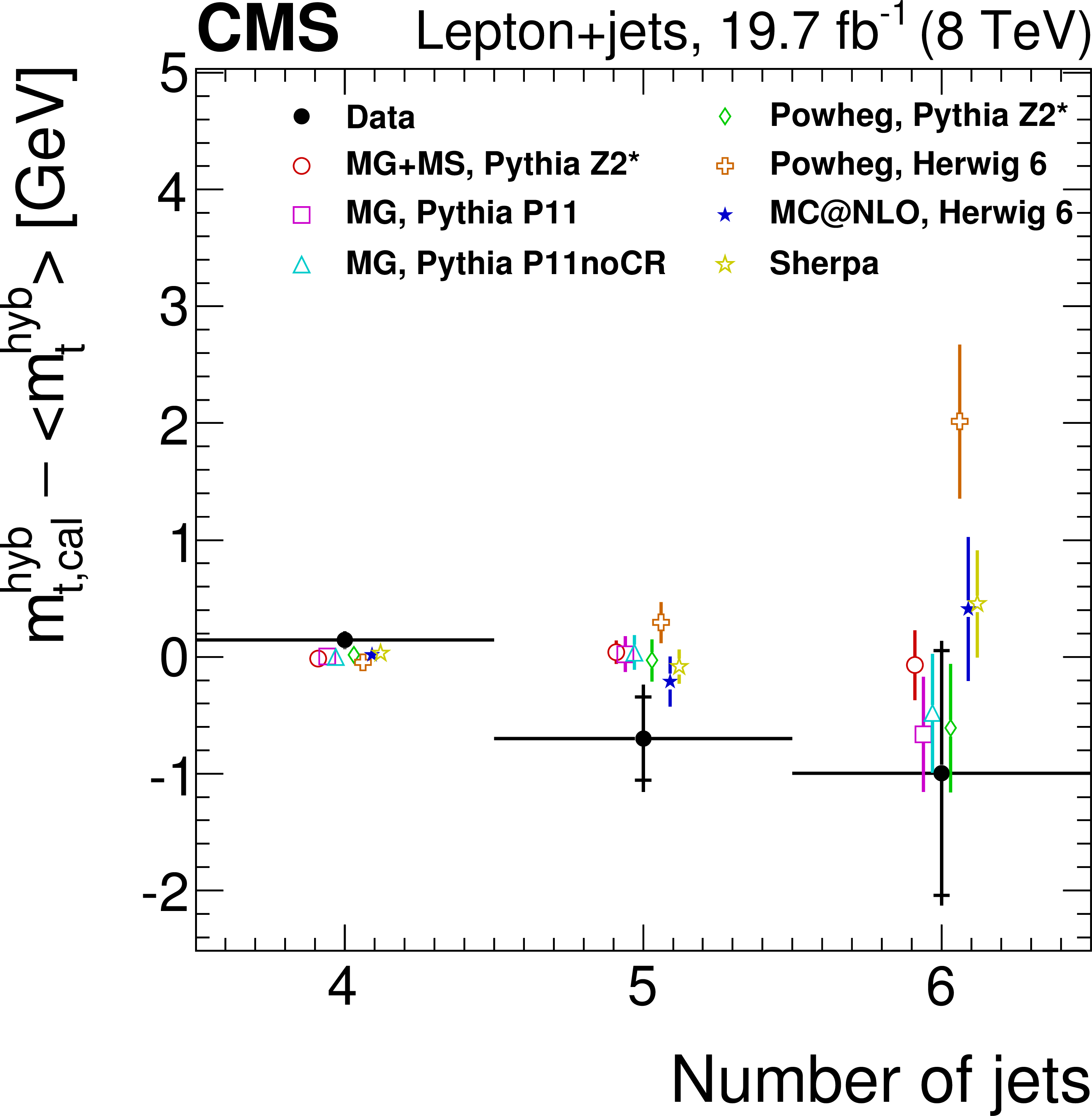
Figure 9-d:
Measurement of the number of jets with $ {p_{\mathrm {T}}} >$ 30 GeV. The filled circles represent the data, and the other symbols are for the simulations. For reasons of clarity the horizontal error bars are shown only for the data points and each of the simulations is shown as a single offset point with a vertical error bar representing its statistical uncertainty. The statistical uncertainty of the data is displayed by the inner error bars. For the outer error bars, the systematic uncertainties are added in quadrature. The open circles correspond to MadGraph with the PYTHIA Z2* tune, the open squares to MadGraph with the PYTHIA Perugia 2011 tune, and the open triangles represent MadGraph with the PYTHIA Perugia 2011 noCR tune. The open diamonds correspond to POWHEG with the PYTHIA Z2* tune and the open crosses correspond to POWHEG with HERWIG 6. The filled stars are for MC@NLO with HERWIG 6 and the open stars are for SHERPA. |
png pdf |
Figure 10:
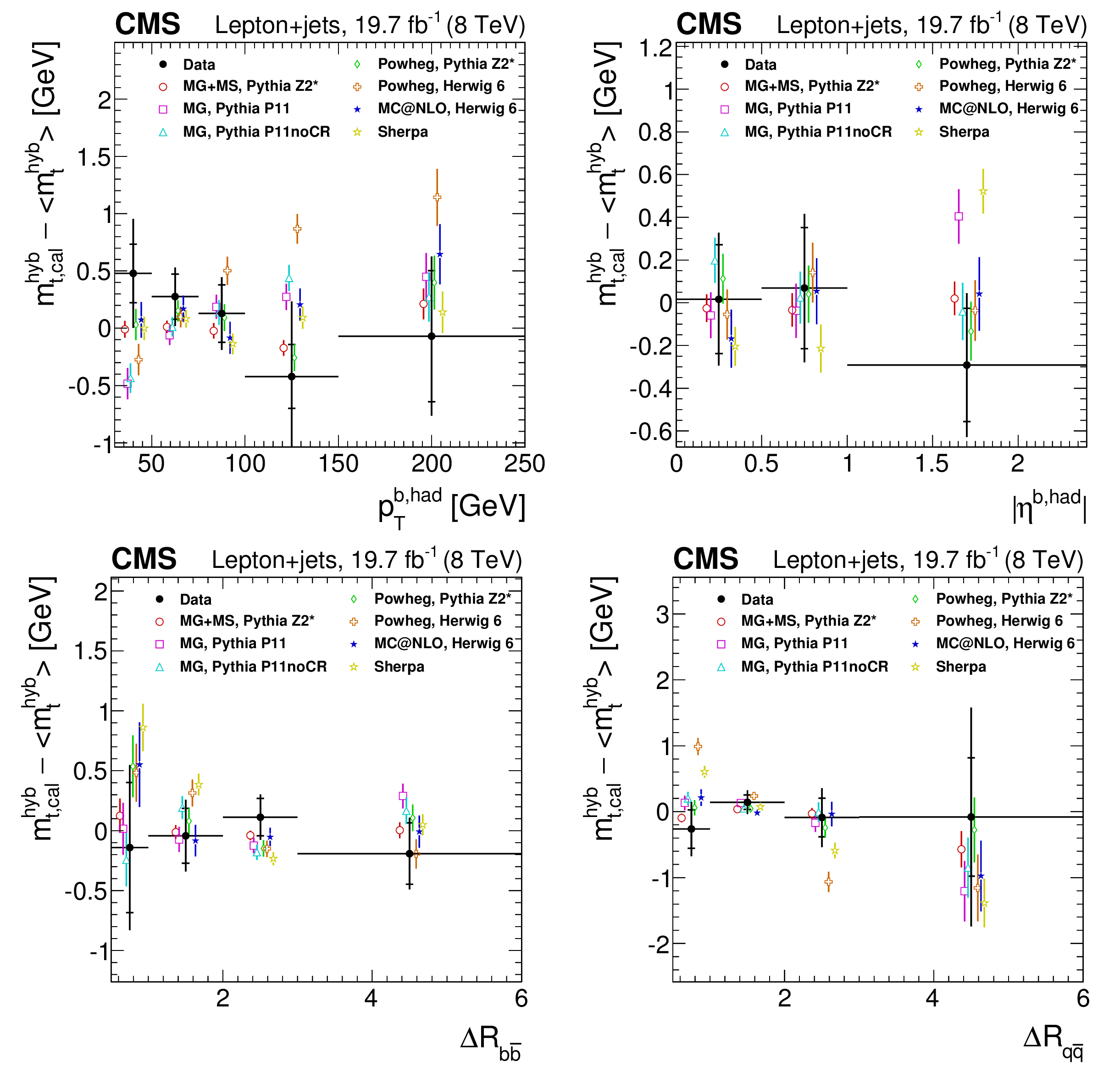
Measurements of $ {m_{ {\mathrm {t}} }} $ as a function of the $ {p_{\mathrm {T}}} $ of the b jet assigned to the hadronic decay branch ($ {p_{\mathrm {T}}} ^{\rm {b,had}}$), the pseudorapidity of the b jet assigned to the hadronic decay branch ($\left |\eta ^{\rm b,had}\right |$), the $\Delta R$ between the b jets ($\Delta R_{ { {\mathrm {b}} {\overline {\mathrm {b}}} } }$), and the $\Delta R$ between the light-quark jets ($\Delta R_{ { {\mathrm {q}} {\overline {\mathrm {q}}} } }$). The filled circles represent the data, and the other symbols are for the simulations. For reasons of clarity the horizontal error bars are shown only for the data points and each of the simulations is shown as a single offset point with a vertical error bar representing its statistical uncertainty. The statistical uncertainty of the data is displayed by the inner error bars. For the outer error bars, the systematic uncertainties are added in quadrature.The open circles correspond to MadGraph with the PYTHIA Z2* tune, the open squares to MadGraph with the PYTHIA Perugia 2011 tune, and the open triangles represent MadGraph with the PYTHIA Perugia 2011 noCR tune. The open diamonds correspond to POWHEG with the PYTHIA Z2* tune and the open crosses correspond to POWHEG with HERWIG 6. The filled stars are for MC@NLO with HERWIG 6 and the open stars are for SHERPA. |

png pdf |
Figure 10-a:
Measurement of $ {m_{ {\mathrm {t}} }} $ as a function of the $ {p_{\mathrm {T}}} $ of the b jet assigned to the hadronic decay branch ($ {p_{\mathrm {T}}} ^{\rm {b,had}}$). The filled circles represent the data, and the other symbols are for the simulations. For reasons of clarity the horizontal error bars are shown only for the data points and each of the simulations is shown as a single offset point with a vertical error bar representing its statistical uncertainty. The statistical uncertainty of the data is displayed by the inner error bars. For the outer error bars, the systematic uncertainties are added in quadrature.The open circles correspond to MadGraph with the PYTHIA Z2* tune, the open squares to MadGraph with the PYTHIA Perugia 2011 tune, and the open triangles represent MadGraph with the PYTHIA Perugia 2011 noCR tune. The open diamonds correspond to POWHEG with the PYTHIA Z2* tune and the open crosses correspond to POWHEG with HERWIG 6. The filled stars are for MC@NLO with HERWIG 6 and the open stars are for SHERPA. |
png pdf |
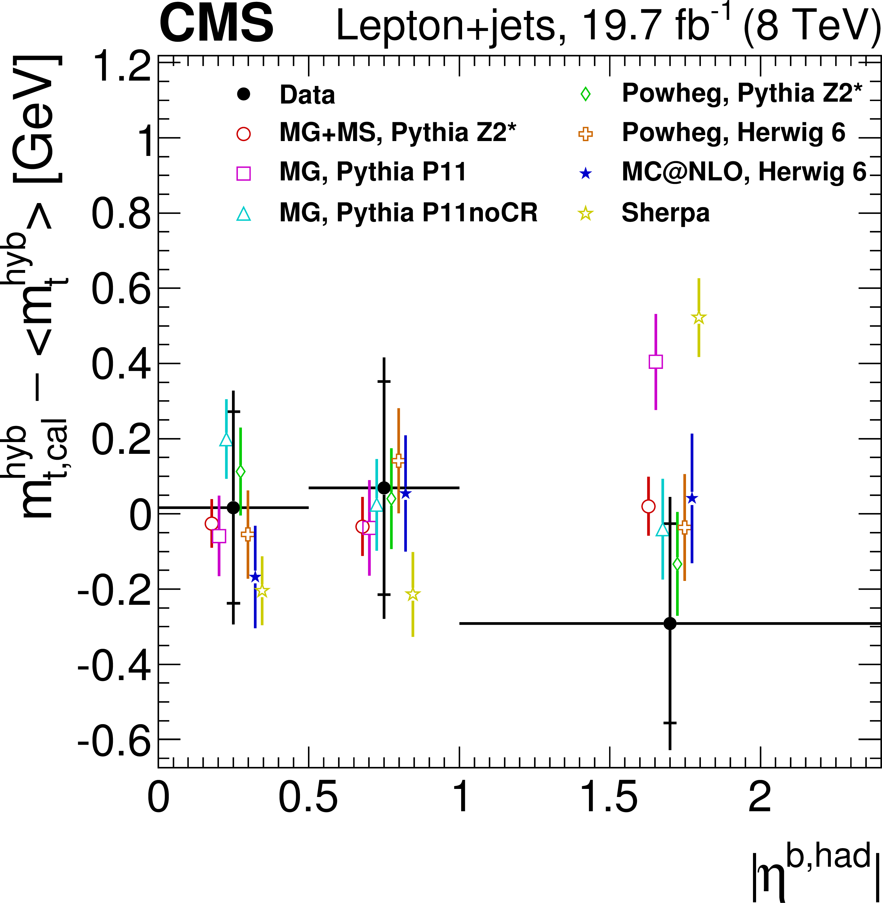
Figure 10-b:
Measurement of $ {m_{ {\mathrm {t}} }} $ as a function of the pseudorapidity of the b jet assigned to the hadronic decay branch ($\left |\eta ^{\rm b,had}\right |$). The filled circles represent the data, and the other symbols are for the simulations. For reasons of clarity the horizontal error bars are shown only for the data points and each of the simulations is shown as a single offset point with a vertical error bar representing its statistical uncertainty. The statistical uncertainty of the data is displayed by the inner error bars. For the outer error bars, the systematic uncertainties are added in quadrature.The open circles correspond to MadGraph with the PYTHIA Z2* tune, the open squares to MadGraph with the PYTHIA Perugia 2011 tune, and the open triangles represent MadGraph with the PYTHIA Perugia 2011 noCR tune. The open diamonds correspond to POWHEG with the PYTHIA Z2* tune and the open crosses correspond to POWHEG with HERWIG 6. The filled stars are for MC@NLO with HERWIG 6 and the open stars are for SHERPA. |

png pdf |
Figure 10-c:
Measurement of $ {m_{ {\mathrm {t}} }} $ as a function of the $\Delta R$ between the b jets ($\Delta R_{ { {\mathrm {b}} {\overline {\mathrm {b}}} } }$). The filled circles represent the data, and the other symbols are for the simulations. For reasons of clarity the horizontal error bars are shown only for the data points and each of the simulations is shown as a single offset point with a vertical error bar representing its statistical uncertainty. The statistical uncertainty of the data is displayed by the inner error bars. For the outer error bars, the systematic uncertainties are added in quadrature.The open circles correspond to MadGraph with the PYTHIA Z2* tune, the open squares to MadGraph with the PYTHIA Perugia 2011 tune, and the open triangles represent MadGraph with the PYTHIA Perugia 2011 noCR tune. The open diamonds correspond to POWHEG with the PYTHIA Z2* tune and the open crosses correspond to POWHEG with HERWIG 6. The filled stars are for MC@NLO with HERWIG 6 and the open stars are for SHERPA. |

png pdf |
Figure 10-d:
Measurement of $ {m_{ {\mathrm {t}} }} $ as a function of the $\Delta R$ between the light-quark jets ($\Delta R_{ { {\mathrm {q}} {\overline {\mathrm {q}}} } }$). The filled circles represent the data, and the other symbols are for the simulations. For reasons of clarity the horizontal error bars are shown only for the data points and each of the simulations is shown as a single offset point with a vertical error bar representing its statistical uncertainty. The statistical uncertainty of the data is displayed by the inner error bars. For the outer error bars, the systematic uncertainties are added in quadrature.The open circles correspond to MadGraph with the PYTHIA Z2* tune, the open squares to MadGraph with the PYTHIA Perugia 2011 tune, and the open triangles represent MadGraph with the PYTHIA Perugia 2011 noCR tune. The open diamonds correspond to POWHEG with the PYTHIA Z2* tune and the open crosses correspond to POWHEG with HERWIG 6. The filled stars are for MC@NLO with HERWIG 6 and the open stars are for SHERPA. |

png pdf |
Figure 11:
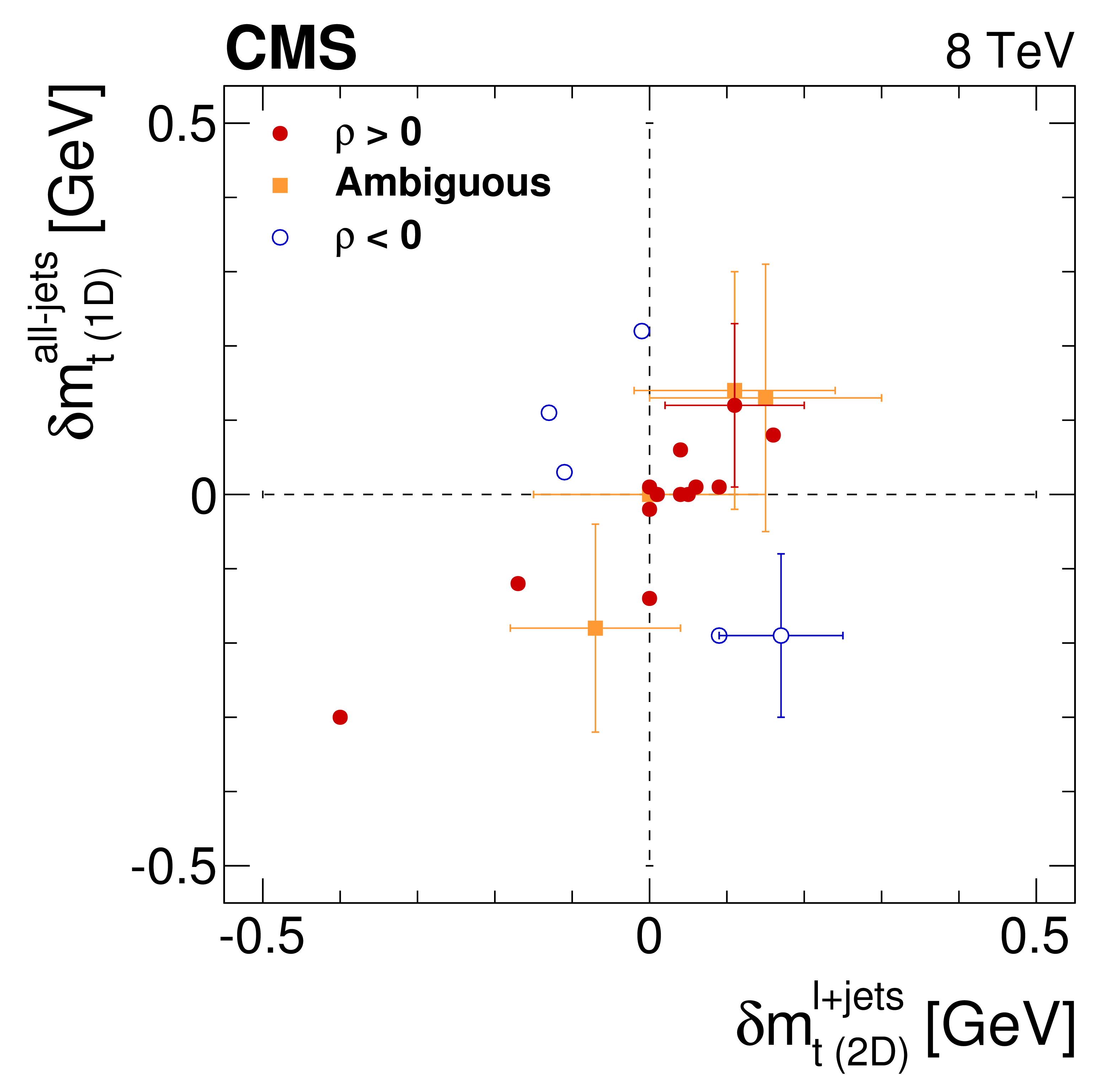
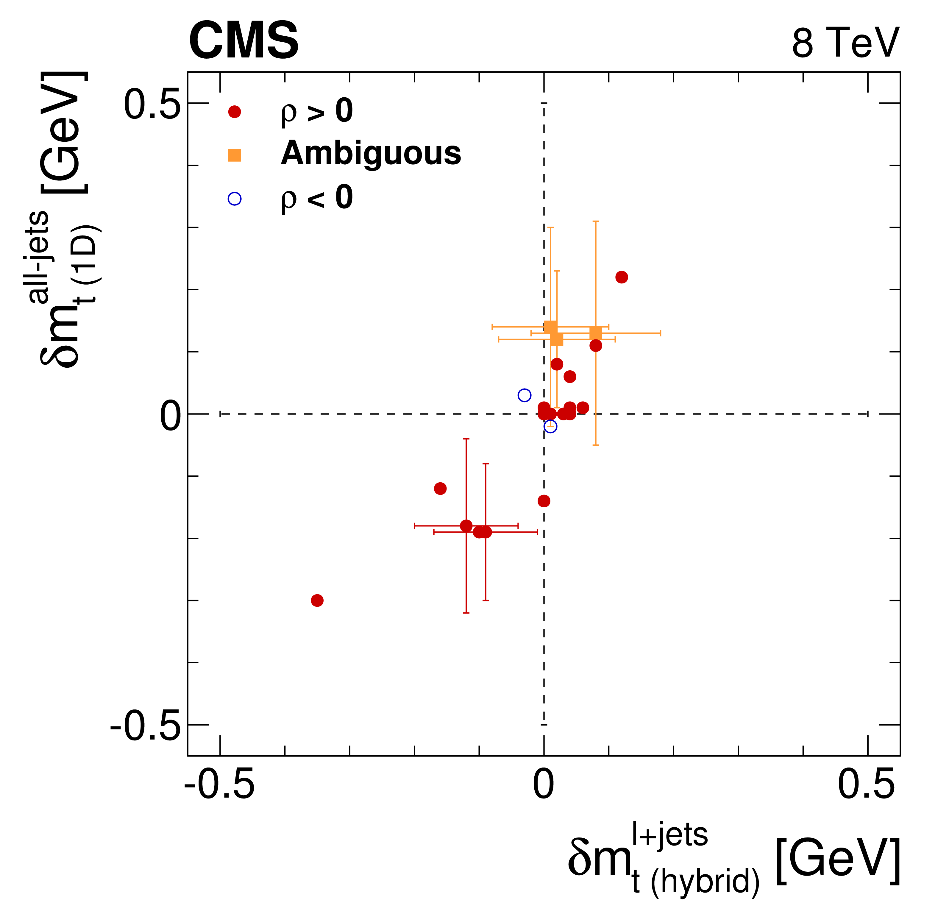
Systematic uncertainty correlations for mass measurements in the lepton+jets and all-jets channels. Each point represents a single systematic uncertainty taken from Tables 1 and 2. Left panel: for the 2D lepton+jets and 1D all-jets measurements; Right panel: for the hybrid lepton+jets and the 1D all-jets measurements. The filled circles correspond to the systematic uncertainties which show a positive correlation between the two fit methods and the open circles to the systematic terms which show a negative correlation. The points shown as filled squares are those for which the systematic estimation is dominated by a statistical uncertainty, so no clear categorization is possible. The vertical and horizontal error bars correspond to the statistical uncertainties in the systematic uncertainties. |
png pdf |
Figure 11-a:
Systematic uncertainty correlations for mass measurements in the lepton+jets and all-jets channels. Each point represents a single systematic uncertainty taken from Tables 1 and 2 for the 2D lepton+jets and 1D all-jets measurements. The filled circles correspond to the systematic uncertainties which show a positive correlation between the two fit methods and the open circles to the systematic terms which show a negative correlation. The points shown as filled squares are those for which the systematic estimation is dominated by a statistical uncertainty, so no clear categorization is possible. The vertical and horizontal error bars correspond to the statistical uncertainties in the systematic uncertainties. |
png pdf |
Figure 11-b:
Systematic uncertainty correlations for mass measurements in the lepton+jets and all-jets channels. Each point represents a single systematic uncertainty taken from Tables 1 and 2 for the hybrid lepton+jets and the 1D all-jets measurements. The filled circles correspond to the systematic uncertainties which show a positive correlation between the two fit methods and the open circles to the systematic terms which show a negative correlation. The points shown as filled squares are those for which the systematic estimation is dominated by a statistical uncertainty, so no clear categorization is possible. The vertical and horizontal error bars correspond to the statistical uncertainties in the systematic uncertainties. |

png pdf |
Figure 12:
Summary of the CMS $ {m_{ {\mathrm {t}} }} $ measurements and their combination. The thick error bars show the statistical uncertainty and the thin error bars show the total uncertainty. Also shown are the current Tevatron [8] and world average [7] combinations. |

png pdf |
Figure 13:
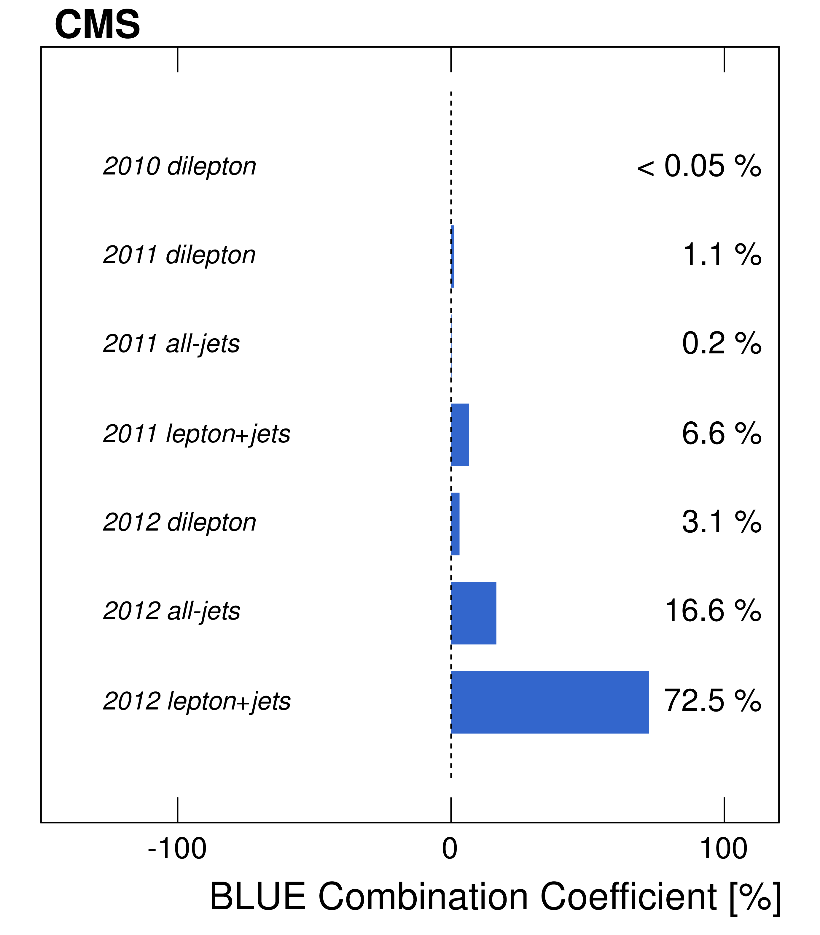
Results of the BLUE combining procedure on the CMS measurements showing (left) the combination coefficients, and (right) the pulls for each contribution. |
png pdf |
Figure 13-a:
Results of the BLUE combining procedure on the CMS measurements showing the combination coefficients for each contribution. |

png pdf |
Figure 13-b:
Results of the BLUE combining procedure on the CMS measurements showing the pulls for each contribution. |
png pdf |
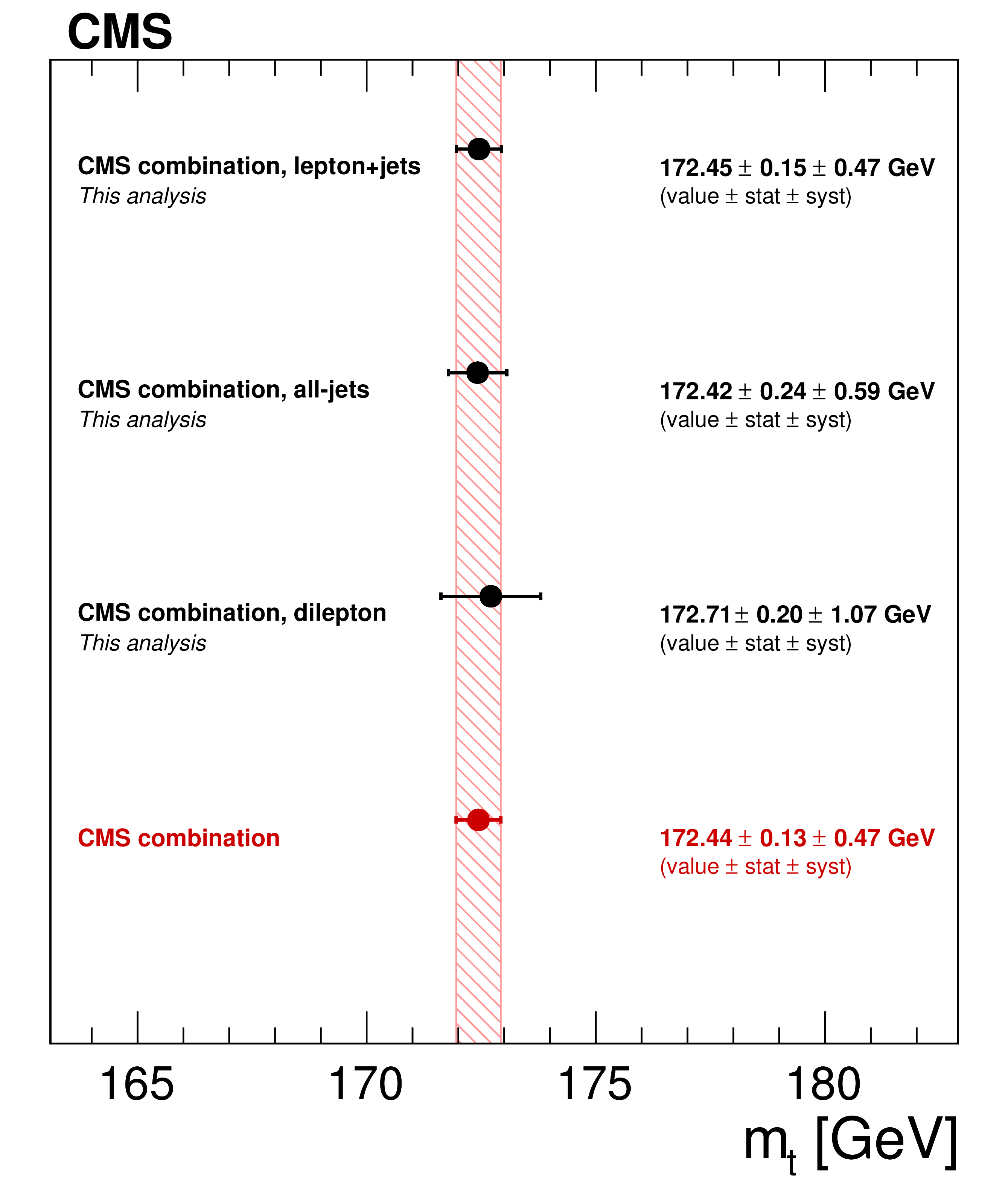
Figure 14:
The combined $\sqrt {s} =$ 7 and 8 TeV measurements of $ {m_{ {\mathrm {t}} }} $ for each of the $ {\mathrm {t}\overline {\mathrm {t}}} $ decay channels. |
| Tables | |

png pdf |
Table 1:
Category breakdown of the systematic uncertainties for the 2D, 1D, and hybrid measurements in the lepton+jets channel. Each term has been estimated using the procedures described in Section 6. The uncertainties are expressed in GeV and the signs are taken from the $+1\sigma $ shift in the value of the quantity. Thus a positive sign indicates an increase in the value of $m_{ {\mathrm {t}} }$ or the JSF and a negative sign indicates a decrease. With the exception of the flavor-dependent JEC terms (see Section 6), the total systematic uncertainty is obtained from the sum in quadrature of the individual systematic uncertainties. |

png pdf |
Table 2:
Category breakdown of the systematic uncertainties for the 2D, 1D and hybrid measurements in the all-jets channel. Each term has been estimated using the procedures described in Section 6. The uncertainties are expressed in GeV and the signs are taken from the $+1\sigma $ shift in the value of the quantity. Thus a positive sign indicates an increase in the value of $m_{ {\mathrm {t}} }$ or the JSF and a negative sign indicates a decrease. With the exception of the flavor-dependent JEC terms (see Section 6), the total systematic uncertainty is obtained from the sum in quadrature of the individual systematic uncertainties. |
png pdf |
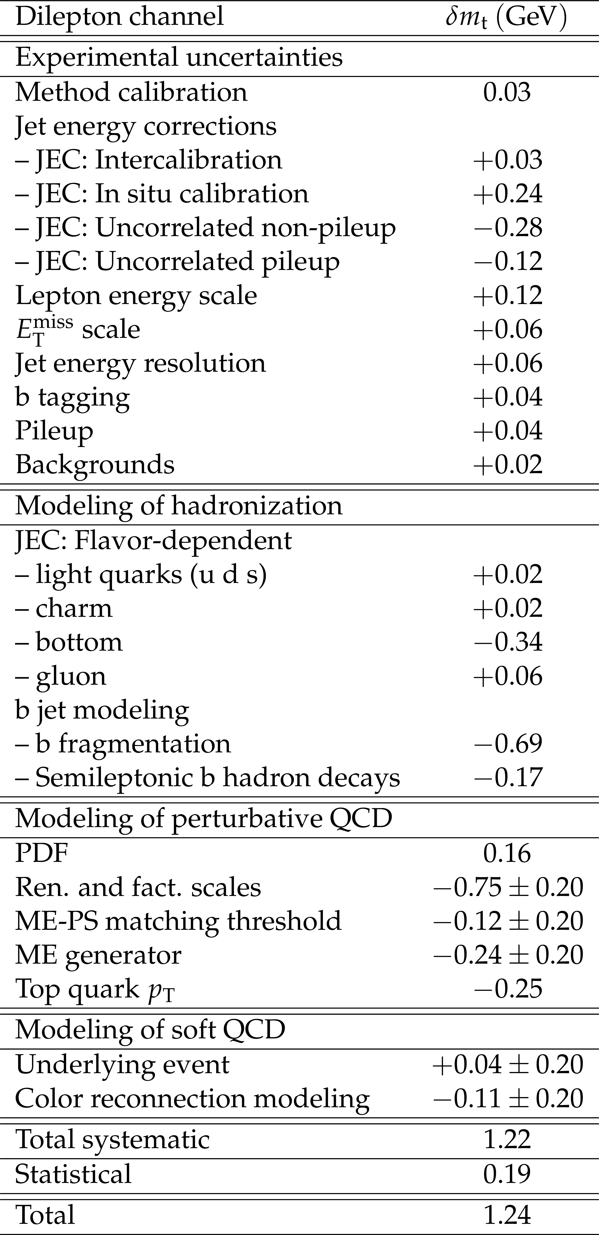
Table 3:
Category breakdown of the systematic uncertainties for the AMWT measurement in the dilepton channel. Each term has been estimated using the procedures described in Section 6. The uncertainties are expressed in GeV and the signs are taken from the $+1\sigma $ shift in the value of the quantity. Thus a positive sign indicates an increase in the value of $m_{ {\mathrm {t}} }$ and a negative sign indicates a decrease. With the exception of the flavor-dependent JEC terms (see Section 6), the total systematic uncertainty is obtained from the sum in quadrature of the individual systematic uncertainties. |
png pdf |
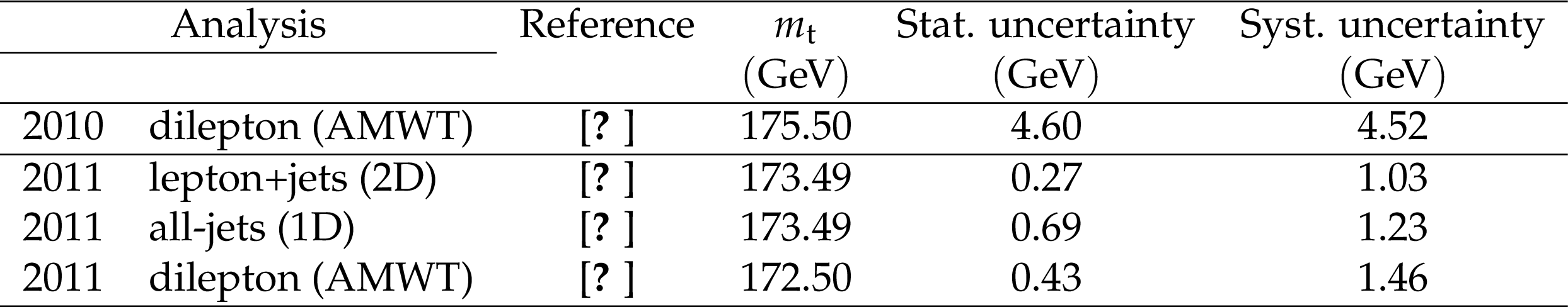
Table 4:
CMS measurements of the top quark mass using the data recorded at $\sqrt {s} =$ 7 TeV. |

png pdf |
Table 5:
Comparison of different simulations and the data. The summed $\chi ^{2}$ values and number of standard deviations are computed for the 27 points entering Figs. 9 and 10 assuming two-sided Gaussian statistics. |

png pdf |
Table 6:
Nominal correlation coefficients for the systematic uncertainties. The term $\rho _{\rm chan}$ is the correlation factor for measurements in the same top quark decay channel, but different years and the term $\rho _{\rm year}$ is the correlation between measurements in different channels from the same year. |

png pdf |
Table 7:
Combination results for the permutations of the 2D, 1D, and hybrid measurements. The permutation order is defined to be lepton+jets:all-jets:dilepton, thus 211 corresponds to the 2D lepton+jets:1D all-jets:AMWT dilepton combination. |
png pdf |
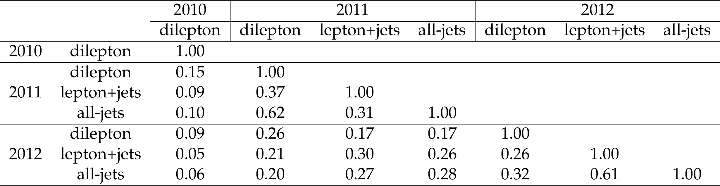
Table 8:
Correlations between input measurements. The elements in the table are labelled according to the analysis they correspond to (rows and columns read as 2010, 2011, 2012 followed by the $ {\mathrm {t}\overline {\mathrm {t}}} $ decay channel name). |

png pdf |
Table 9:
Category breakdown of systematic uncertainties for the combined mass result. The uncertainties are expressed in GeV. |
| Summary |
|
A new set of measurements of the top quark mass has been presented, based on the data recorded by the CMS experiment at the LHC at $\sqrt{s} =$ 8 TeV during 2012, and corresponding to a luminosity of 19.7 fb$^{-1}$. The top quark mass has been measured in the lepton+jets, all-jets and dilepton decay channels, giving values of 172.32 $\pm$ 0.25 (stat) $\pm$ 0.59 (syst) GeV, and 172.82 $\pm$ 0.19 (stat) $\pm$ 1.22 (syst) GeV, respectively. Individually, these constitute the most precise measurements in each of the decay channels studied. When combined with the published CMS results at $\sqrt{s} =$ 7 TeV, a top quark mass measurement of is obtained. This is the most precise measurement of $m_{\text{top}}$ to date, with a total uncertainty of 0.48 GeV, and it supersedes all of the previous CMS measurements of the top quark mass. The top quark mass has also been studied as a function of the event kinematical properties in the lepton+jets channel. No indications of a kinematical bias in the measurements is observed and the data are consistent with a range of predictions from current theoretical models of $ \mathrm{ t \bar{t} } $ production. |
| References | ||||
| 1 | ALEPH, CDF, D0, DELPHI, L3, OPAL and SLD Collaborations, the LEP Electroweak Working Group, the Tevatron Electroweak Working Group and the SLD Electroweak and Heavy Flavour Groups | Precision electroweak measurements and constraints on the Standard Model | 1012.2367 | |
| 2 | M. Baak et al. | The electroweak fit of the standard model after the discovery of a new boson at the LHC | EPJC 72 (2012) 2205, , Updates available from http://gfitter.desy.de | 1209.2716 |
| 3 | G. Degrassi et al. | Higgs mass and vacuum stability in the Standard Model at NNLO | JHEP 08 (2012) 1 | 1205.6497 |
| 4 | F. Bezrukov, M. Y. Kalmykov, B. A. Kniehl, and M. Shaposhnikov | Higgs boson mass and new physics | JHEP 10 (2012) 140 | 1205.2893 |
| 5 | F. Bezrukov and M. Shaposhnikov | The Standard Model Higgs boson as the inflaton | PLB 659 (2008) 703 | 0710.3755 |
| 6 | A. D. Simone, M. P. Herzberg, and F. Wilczek | Running inflation in the Standard Model | PLB 678 (2009) 1 | 0812.4946 |
| 7 | ATLAS, CDF, CMS and D0 Collaborations | First combination of Tevatron and LHC measurements of the top quark mass | 1403.4427 | |
| 8 | The Tevatron Electroweak Working Group | Combination of the CDF and D0 results on the mass of the top quark using up to $ 9.7\,\text{fb}^{-1} $ at the Tevatron | 1407.2682 | |
| 9 | ATLAS Collaboration | Measurement of the top quark mass in the $ t\bar{t}\rightarrow \text{ lepton+jets } $ and $ t\bar{t}\rightarrow \text{ dilepton } $ channels using $ \sqrt{s}=7 $ $ {\mathrm { TeV}} $ ATLAS data | EPJC 75 (2015) 330 | 1503.05427 |
| 10 | A. H. Hoang and I. W. Stewart | Top Mass Measurements from Jets and the Tevatron Top Quark Mass | NPPS 185 (2008) 220 | 0808.0222 |
| 11 | V. Ahrens et al. | Precision predictions for the $ t \bar{t} $ production cross section at hadron colliders | PLB 703 (2011) 135 | 1105.5824 |
| 12 | A. Buckley et al. | General-purpose event generators for LHC physics | PR 504 (2011) 145 | 1101.2599 |
| 13 | CMS Collaboration | The CMS experiment at the CERN LHC | JINST 3 (2008) S08004 | CMS-00-001 |
| 14 | J. Alwall et al. | MadGraph 5: going beyond | JHEP 06 (2011) 128 | 1106.0522 |
| 15 | P. Artoisenet, R. Frederix, O. Mattelaer, and R. Rietkerk | Automatic spin-entangled decays of heavy resonances in Monte Carlo simulations | JHEP 03 (2013) 015 | 1212.3460 |
| 16 | T. Sj\"ostrand, S. Mrenna, and P. Skands | PYTHIA 6.4 physics and manual | JHEP 05 (2006) 026 | hep-ph/0603175 |
| 17 | S. Jadach, Z. W\cas, R. Decker, and J. H. K\"uhn | The tau decay library TAUOLA: Version 2.4 | CPC 76 (1993) 361 | |
| 18 | R. Field | Early LHC Underlying Event Data - Findings and Surprises | 1010.3558 | |
| 19 | J. Pumplin et al. | New generation of parton distributions with uncertainties from global QCD analysis | JHEP 07 (2002) 012 | hep-ph/0201195 |
| 20 | GEANT4 Collaboration | GEANT4---a simulation toolkit | NIMA 506 (2003) 250 | |
| 21 | S. Alioli, P. Nason, C. Oleari, and E. Re | NLO single-top production matched with shower in POWHEG: $ s $- and $ t $-channel contributions | JHEP 09 (2009) 111 | 0907.4076 |
| 22 | E. Re | Single-top $ W $ $ t $-channel production matched with parton showers using the POWHEG method | EPJC 71 (2011) 1547 | 1009.2450 |
| 23 | P. Nason | A new method for combining NLO QCD with shower Monte Carlo algorithms | JHEP 11 (2004) 040 | hep-ph/0409146 |
| 24 | S. Frixione, P. Nason, and C. Oleari | Matching NLO QCD computations with parton shower simulations: the POWHEG method | JHEP 11 (2007) 070 | 0709.2092 |
| 25 | S. Alioli, P. Nason, C. Oleari, and E. Re | A general framework for implementing NLO calculations in shower Monte Carlo programs: the POWHEG BOX | JHEP 06 (2010) 043 | 1002.2581 |
| 26 | N. Kidonakis | Next-to-next-to-leading soft-gluon corrections for the top quark cross section and transverse momentum distribution | PRD 82 (2010) 114030 | 1009.4935 |
| 27 | N. Kidonakis | Differential and total cross sections for top pair and single top production | 1205.3453 | |
| 28 | K. Melnikov and F. Petriello | Electroweak gauge boson production at hadron colliders through $ O(\alpha_s^2) $ | PRD 74 (2006) 114017 | hep-ph/0609070 |
| 29 | J. M. Campbell and R. K. Ellis | MCFM for the Tevatron and the LHC | NPPS 205-206 (2010) 10 | 1007.3492 |
| 30 | M. Czakon, P. Fiedler, and A. Mitov | The total top quark pair production cross-section at hadron colliders through O($ \alpha_S^4 $) | PRL 110 (2013) 252004 | 1303.6254 |
| 31 | CMS Collaboration | Particle--Flow Event Reconstruction in CMS and Performance for Jets, Taus, and $ E_{\mathrm{T}}^{\text{miss}} $ | CDS | |
| 32 | CMS Collaboration | Commissioning of the Particle-flow Event Reconstruction with the first LHC collisions recorded in the CMS detector | CDS | |
| 33 | CMS Collaboration | Performance of electron reconstruction and selection with the CMS detector in proton-proton collisions at $ \sqrt{s} = 8 $$ TeV $ | JINST 6 (2015) P06005 | CMS-EGM-13-001 1502.02701 |
| 34 | CMS Collaboration | Performance of CMS muon reconstruction in pp collision events at $ \sqrt{s} = 7 $$ TeV $ | JINST 7 (2012) P10002 | |
| 35 | M. Cacciari, G. P. Salam, and G. Soyez | The anti-$ k_t $ jet clustering algorithm | JHEP 04 (2008) 063 | 0802.1189 |
| 36 | M. Cacciari, G. P. Salam, and G. Soyez | FastJet user manual | EPJC 72 (2012) 1896 | 1111.6097 |
| 37 | CMS Collaboration | Determination of jet energy calibration and transverse momentum resolution in CMS | JINST 6 (2011) P11002 | CMS-JME-10-011 1107.4277 |
| 38 | CMS Collaboration | Performance of b tagging at $ \sqrt{s}=8 $ TeV in multijet, $ \rm{t}\overline{\rm t} $ and boosted topology events | CMS-PAS-BTV-13-001 | CMS-PAS-BTV-13-001 |
| 39 | CMS Collaboration | Measurement of the differential cross section for top quark pair production in pp collisions at $ \sqrt{s} = 8 $ TeV | Submitted to EPJC | CMS-TOP-12-028 1505.04480 |
| 40 | D0 Collaboration | Direct measurement of the top quark mass at D0 | PRD 58 (1998) 052001 | hep-ex/9801025 |
| 41 | Particle Data Group, K. A. Olive et al. | Review of Particle Physics | CPC 38 (2014) 090001 | |
| 42 | D0 Collaboration | Measurement of the top quark mass using dilepton events | PRL 80 (1998) 2063 | hep-ex/9706014 |
| 43 | CMS Collaboration | Measurement of the top-quark mass in $ \mathrm{ t \bar{t} }\ $ events with dilepton final states in pp collisions at $ \sqrt{s} = $ 7 TeV | EPJC 72 (2012) 2202 | |
| 44 | L. Sonnenschein | Algebraic approach to solve $ \mathrm{ t \bar{t} } $ dilepton equations | PRD 72 (2005) 095020 | hep-ph/0510100 |
| 45 | L. Sonnenschein | Analytical solution of $ \mathrm{ t \bar{t} } $ dilepton equations | PRD 73 (2006) 054015, , [Erratum: \DOI10.1103/PhysRevD.73.054015] | hep-ph/060311 |
| 46 | R. H. Dalitz and G. R. Goldstein | Decay and polarization properties of the top quark | PRD 45 (1992) 1531 | |
| 47 | J. D'Hondt et al. | Fitting of Event Topologies with External Kinematic Constraints in CMS | CMS-NOTE-2006-023 | |
| 48 | CMS Collaboration | Measurement of the top-quark mass in all-jets $ \mathrm{t}\overline{\mathrm{t}} $ events in pp collisions at $ \sqrt{s}=7 $$ TeV $ | EPJC 74 (2014) 2758 | |
| 49 | M. Botje et al. | The PDF4LHC Working Group Interim Recommendations | 1101.0538 | |
| 50 | P. Z. Skands | Tuning Monte Carlo generators: The Perugia tunes | PRD 82 (2010) 074018 | 1005.3457 |
| 51 | M. B\"ahr et al. | Herwig++ physics and manual | EPJC 58 (2008) 639 | 0803.0883 |
| 52 | ALEPH Collaboration | Study of the fragmentation of b quarks into B mesons at the Z peak | PLB 512 (2001) 30 | hep-ex/0106051 |
| 53 | DELPHI Collaboration | A study of the b-quark fragmentation function with the DELPHI detector at LEP I and an averaged distribution obtained at the Z pole | EPJC 71 (2011) 1557 | 1102.4748 |
| 54 | CMS Collaboration | Measurement of the top-quark pair-production cross section and the top-quark mass in the dilepton channel at $ \sqrt{s} =7 $ TeV | JHEP 07 (2011) 049 | |
| 55 | CMS Collaboration | Measurement of the top-quark mass in $ \mathrm{t}\overline{\mathrm{t}} $ events with lepton+jets final states in pp collisions at $ \sqrt{s}=7 $$ TeV $ | JHEP 12 (2012) 105 | |
| 56 | CMS Collaboration | Measurement of the underlying event activity at the LHC with $ \sqrt{s}= 7 $ TeV and comparison with $ \sqrt{s} = 0.9 $ TeV | JHEP 09 (2011) 109 | CMS-QCD-10-010 1107.0330 |
| 57 | T. Gleisberg et al. | Event generation with SHERPA 1.1 | JHEP 02 (2009) 007 | 0811.4622 |
| 58 | S. Hoeche, F. Krauss, S. Schumann, and F. Siegert | QCD matrix elements and truncated showers | JHEP 05 (2009) 053 | 0903.1219 |
| 59 | G. Corcella et al. | HERWIG 6: an event generator for hadron emission reactions with interfering gluons (including supersymmetric processes) | JHEP 01 (2001) 010 | hep-ph/0011363 |
| 60 | S. Frixione and B. R. Webber | Matching NLO QCD computations and parton shower simulations | JHEP 06 (2002) 029 | hep-ph/0204244 |
| 61 | S. Frixione, P. Nason, and B. R. Webber | Matching NLO QCD and parton showers in heavy flavor production | JHEP 08 (2003) 007 | hep-ph/0305252 |
| 62 | L. Lyons, D. Gibaut, and P. Clifford | How to combine correlated estimates of a single physical quantity | NIMA 270 (1988) 110 | |
|
|
Compact Muon Solenoid LHC, CERN |
|

|

|

|

|

|