Information
LHCb-DP-2022-002
arXiv:2305.10515 [PDF]
(Submitted on 17 May 2023)
Inspire 2660905
Tools
Abstract
The LHCb upgrade represents a major change of the experiment. The detectors have been almost completely renewed to allow running at an instantaneous luminosity five times larger than that of the previous running periods. Readout of all detectors into an all-software trigger is central to the new design, facilitating the reconstruction of events at the maximum LHC interaction rate, and their selection in real time. The experiment's tracking system has been completely upgraded with a new pixel vertex detector, a silicon tracker upstream of the dipole magnet and three scintillating fibre tracking stations downstream of the magnet. The whole photon detection system of the RICH detectors has been renewed and the readout electronics of the calorimeter and muon systems have been fully overhauled. The first stage of the all-software trigger is implemented on a GPU farm. The output of the trigger provides a combination of totally reconstructed physics objects, such as tracks and vertices, ready for final analysis, and of entire events which need further offline reprocessing. This scheme required a complete revision of the computing model and rewriting of the experiment's software.
Figures and captions
|
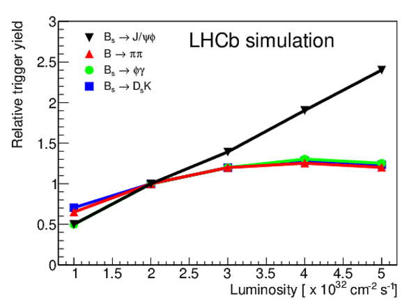
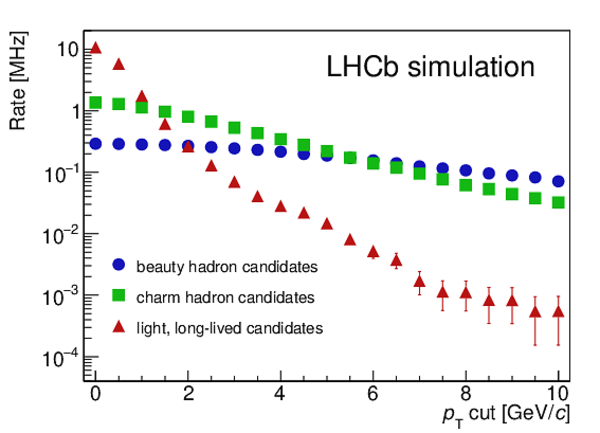
Left: relative trigger yields as a function of instantaneous luminosity, normalised to $\mathcal{L} = 2\times 10^{32}\text{ cm} ^{-2} \text{ s} ^{-1} $. Right: rate of decays reconstructed in the LHCb acceptance as a function of the cut in $ p_{\mathrm{T}}$ of the decaying particle, for decay time $\tau > 0.2\text{ ps} $. |
plot-hans.pdf [14 KiB] HiDef png [159 KiB] Thumbnail [143 KiB] |
|
|
ratesptGP.pdf [15 KiB] HiDef png [189 KiB] Thumbnail [158 KiB] |
|
|
|
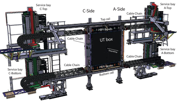
Layout of the upgraded LHCb detector. |
LHCb-u[..].jpg [195 KiB] HiDef png [539 KiB] Thumbnail [161 KiB] |

|
|
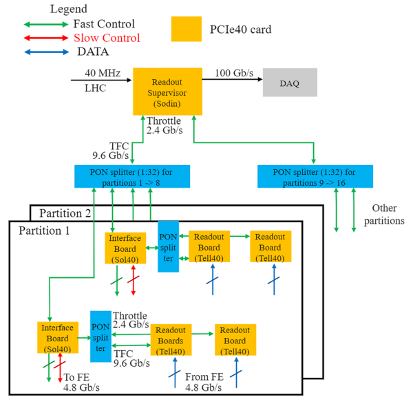
Electronics architecture of the upgraded LHCb experiment. |
electr[..].jpg [313 KiB] HiDef png [370 KiB] Thumbnail [98 KiB] |

|
|
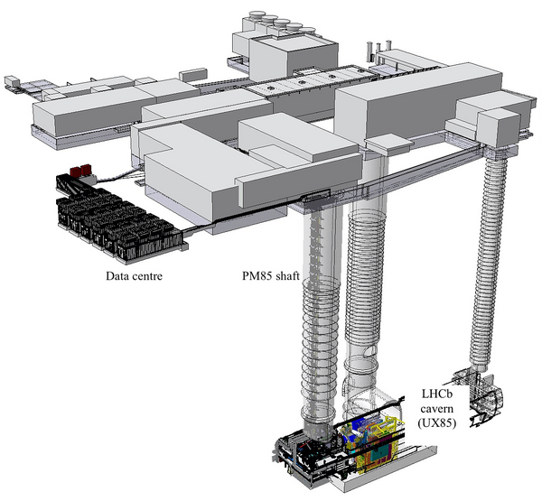
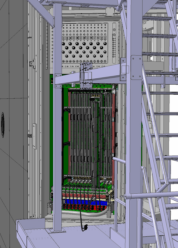
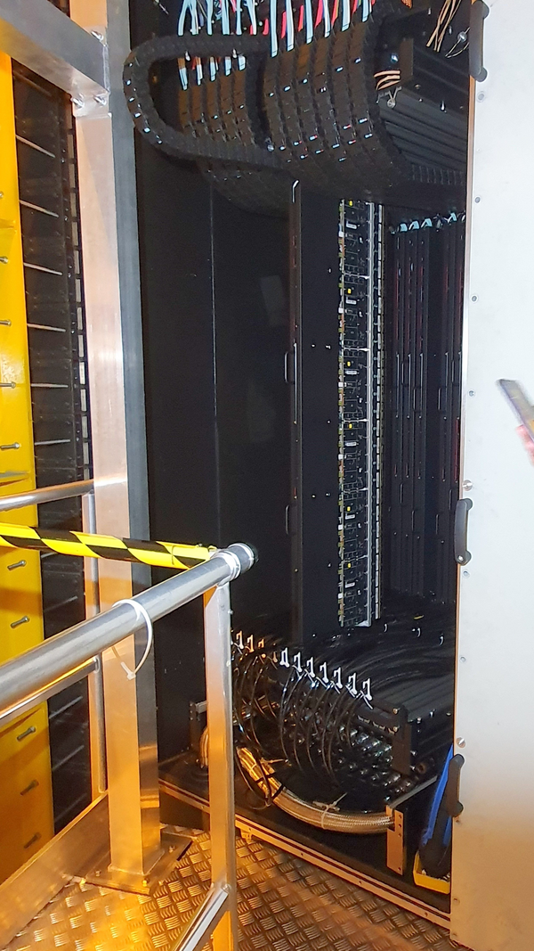
The readout system located in the modular data centre and the front-end electronics in the underground cavern are connected through long-distance optical fibres installed in the PM85 shaft. |
Cavern[..].jpg [307 KiB] HiDef png [784 KiB] Thumbnail [244 KiB] |
|
|
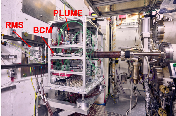
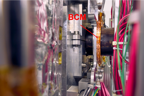
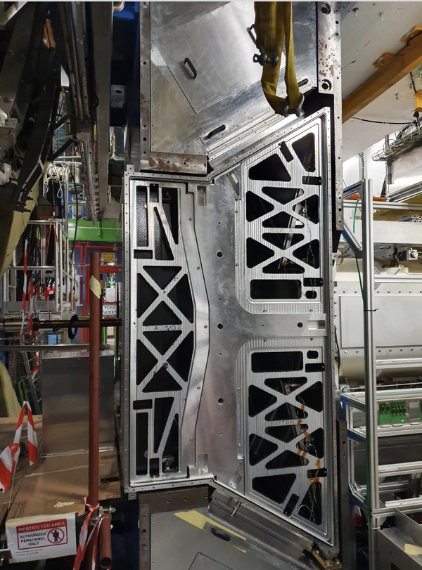
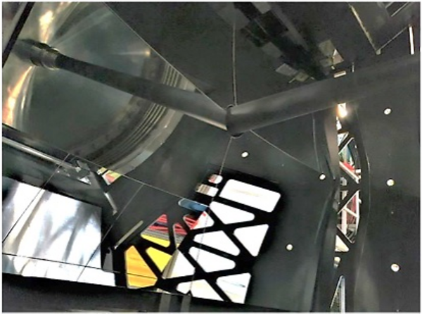
Left: {\gls*{rms}} (under the mylar protection foil at the left side) and {\gls*{plume}} (inside the scaffolding). The arrow indicates the position of {\gls*{bcm}} which is hidden behind the {\gls*{plume}} scaffolding. Right: upstream {\gls*{bcm}} detectors inside their kapton-insulated support surrounding the beam pipe. |
plume-bm.jpg [475 KiB] HiDef png [2 MiB] Thumbnail [452 KiB] |
|
|
BCM.jpg [369 KiB] HiDef png [2 MiB] Thumbnail [350 KiB] |
|
|
|
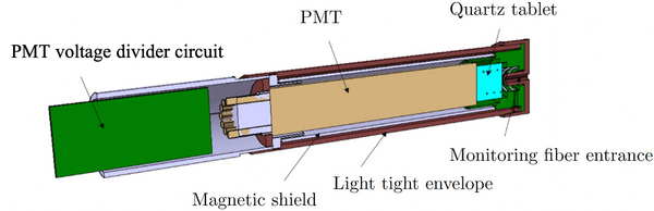
Schematic view of a {\gls*{plume}} elementary detection module. The module is 153 $\text{ mm}$ long and has a diameter of 24 $\text{ mm}$ . |
elem_det_a.jpg [176 KiB] HiDef png [263 KiB] Thumbnail [72 KiB] |
|
|
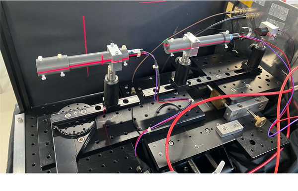
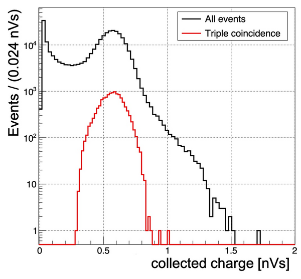
Left: {\gls*{plume}} test beam setup. Right: charge collected by the first {\gls*{pmt}} in the test beam for all events (black line) and events producing a simultaneous signal in the two {\gls*{pmt}} {s} and the trigger (red line). The scale is in nVs where 1 $\text{ nVs}$ = 20 $\text{ pC}$ . |
IMG-TB-new.jpg [402 KiB] HiDef png [1 MiB] Thumbnail [343 KiB] |
|
|
RunID_[..].jpg [145 KiB] HiDef png [291 KiB] Thumbnail [101 KiB] |
|
|
|
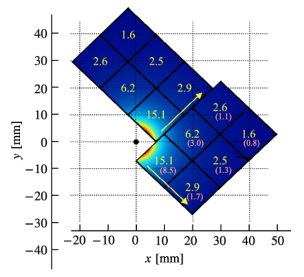
Left: a 3D view of the upgraded {\gls*{velo}} , with cut-out. Some of the new items are highlighted, such as the Side C pixel modules and readout electronics (brown), the Side A RF box (red), the internal gas target system with a storage cell (green), the upstream beam pipe with a sector valve (cyan). Right: data rate per pixel {\gls*{asic}} in $\text{ Gbit/s}$ for the most active module. The numbers in parenthesis are the number of traversing tracks per {\gls*{lhc}} bunch crossing for an average number of interactions per crossing equal to 7.6. Arrows indicate the readout direction. |
dataRa[..].pdf [222 KiB] HiDef png [1 MiB] Thumbnail [564 KiB] |
|
|
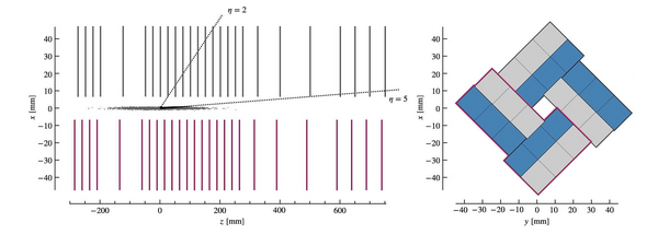
Left: schematic top view of the $z-x$ plane at $y = 0$ (left) with an illustration of the $z$-extent of the luminous region and the nominal LHCb pseudorapidity acceptance, $2<\eta<5$. Right: sketch showing the nominal layout of the {\gls*{asic}} {s} around the $z$ axis in the closed {\gls*{velo}} configuration. Half the {\gls*{asic}} {s} are placed on the upstream module face (grey) and half on the downstream face (blue). The modules on the Side C are highlighted in purple on both sketches. |
zlayou[..].jpg [96 KiB] HiDef png [149 KiB] Thumbnail [48 KiB] |
|
|
Top left: microscope image showing the elongated sensor pixels above the inter- {\gls*{asic}} region. Top right: image highlighting the ion-etched round corner of the sensor. Bottom: schematic of the sensor tile, showing the overall dimensions of the sensor and {\gls*{asic}} . The pixel layout is shown only under {\gls*{asic}} 2. There are $256 \times 256$ active bonded pixels (only every fourth pixel is shown in the figure). An additional row of pixels identified in dark red provides a connection between the {\gls*{asic}} ground and the innermost guard ring of the sensor. Three corners, encircled in red, are shown in detail on the left (A, B, C). |
Schema[..].jpg [129 KiB] HiDef png [1 MiB] Thumbnail [221 KiB] |
|
|
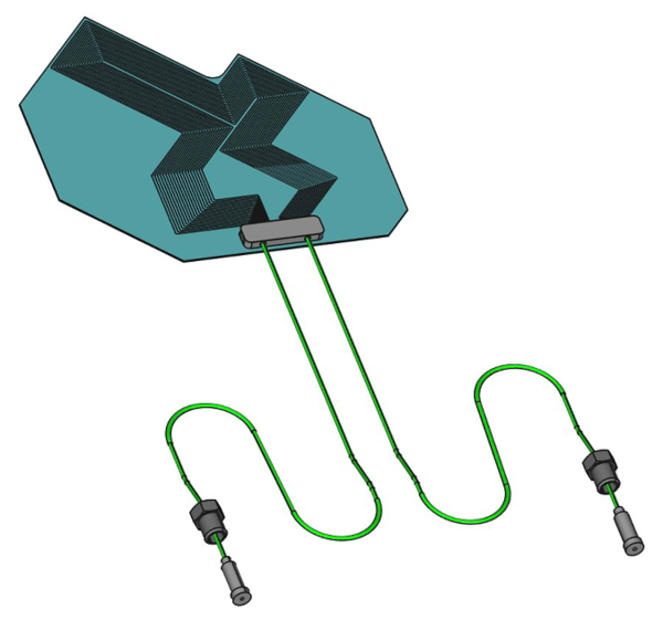
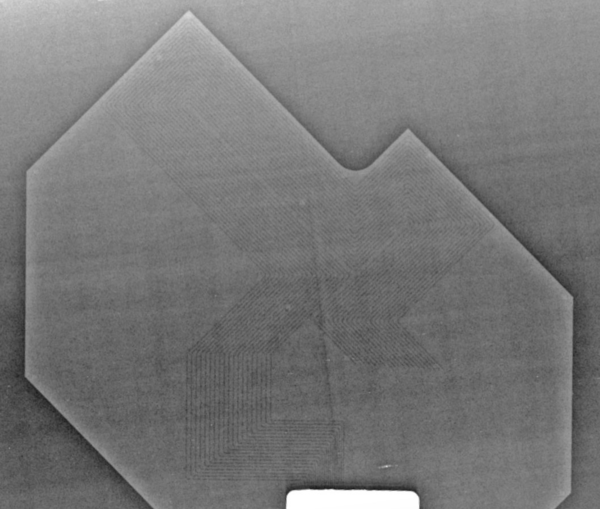
Left: illustration of the silicon microchannel coolers and fluidic connector. Right: the parallel lines represent the etched microchannels, which can be seen in the X-ray image. |
Coolin[..].pdf [71 KiB] HiDef png [1 MiB] Thumbnail [409 KiB] |
|
|
microc[..].pdf [136 KiB] HiDef png [2 MiB] Thumbnail [608 KiB] |
|
|
|
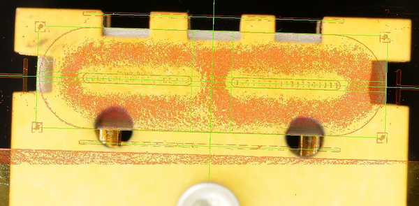
Left: Image of a fluidic connector aligned in the horizontal plane with the corresponding solder layer on the silicon cooler, indicated with the red shadow. Right: X-ray of the solder joint attaching the fluidic connector to the microchannel cooler. No solder has entered the two inlet regions, and no large voids are seen in the solder layer. |
Coolin[..].jpg [205 KiB] HiDef png [1 MiB] Thumbnail [292 KiB] |
|
|
Coolin[..].jpg [219 KiB] HiDef png [196 KiB] Thumbnail [51 KiB] |

|
|
|
Photo of the (left) upstream and (right) downstream faces of a fully-assembled {\gls*{velo}} module. |
module[..].jpg [178 KiB] HiDef png [1 MiB] Thumbnail [269 KiB] |

|
|
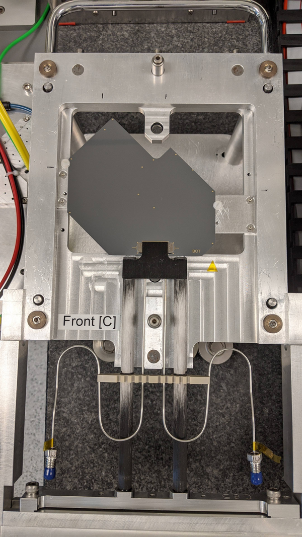
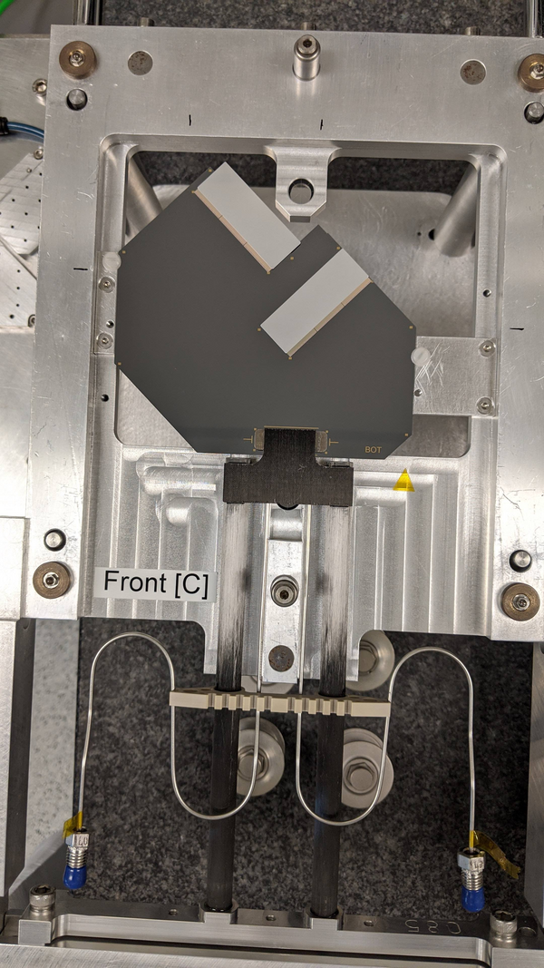
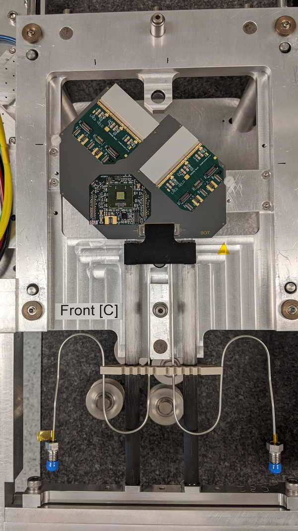
From left to right: bare module; module with tiles; then with hybrids too. |
BareMo[..].jpg [756 KiB] HiDef png [4 MiB] Thumbnail [910 KiB] |
|
|
TilesM[..].jpg [735 KiB] HiDef png [4 MiB] Thumbnail [876 KiB] |
|
|
|
Hybrid[..].jpg [724 KiB] HiDef png [4 MiB] Thumbnail [941 KiB] |
|
|
|
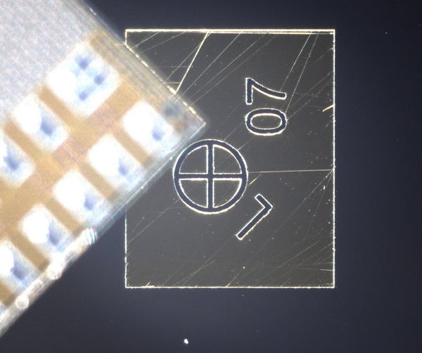
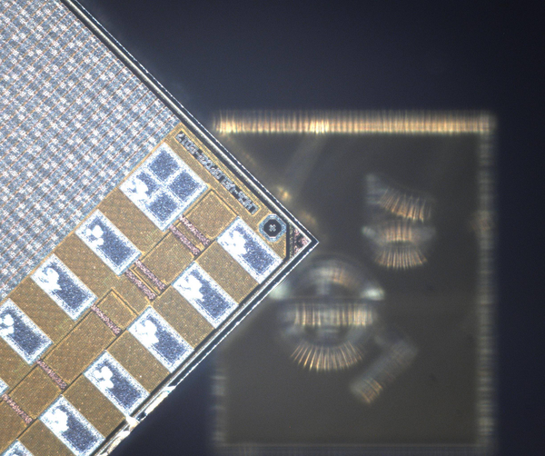
Cross-shaped markers used for module metrology. Left: on the microchannel cooler; centre: on the {\gls*{velopix}} {\gls*{asic}} ; right: on the {\gls*{asic}} -side of the sensor. |
202112[..].jpg [508 KiB] HiDef png [2 MiB] Thumbnail [425 KiB] |
|
|
202112[..].jpg [611 KiB] HiDef png [2 MiB] Thumbnail [499 KiB] |
|
|
|
202112[..].jpg [1 MiB] HiDef png [2 MiB] Thumbnail [573 KiB] |

|
|
|
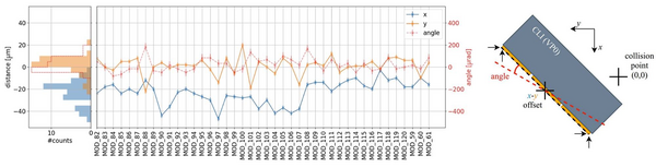
Tile metrology results showing $x$ and $y$ positions and angles for each module. |
TileMe[..].jpg [102 KiB] HiDef png [220 KiB] Thumbnail [74 KiB] |
|
|
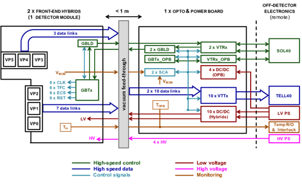
Block diagram showing the main parts of the {\gls*{velo}} electronics system. |
VELOEl[..].pdf [22 KiB] HiDef png [213 KiB] Thumbnail [179 KiB] |
|
|
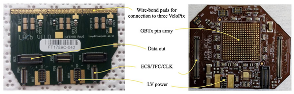
The {\gls*{fend}} (left) and {\gls*{gbtx}} (right) hybrids. |
hybrid[..].jpg [118 KiB] HiDef png [809 KiB] Thumbnail [184 KiB] |
|
|
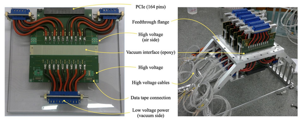
Left: custom-made vacuum feedthrough board. Right: a populated vacuum flange. |
Vacuum[..].jpg [144 KiB] HiDef png [882 KiB] Thumbnail [200 KiB] |
|
|
The Side C half, with 26 modules, ready for the installation into the vacuum vessel. |
halfas[..].jpg [123 KiB] HiDef png [2 MiB] Thumbnail [515 KiB] |

|
|
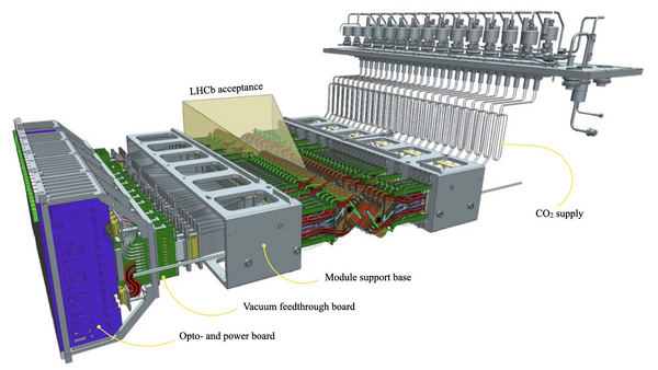
Illustration of the {\gls*{velo}} halves showing modules on the module support bases and the LHCb acceptance as a transparent pyramid. On the left, the flexible electronic cables are shown leading to the vacuum feedthrough boards and {\gls*{opb}} boards in their custom frame. On the right, the flexible construction of long cooling loops is shown as well as the interface between the secondary and isolation vacua, in which sits an array of valves. |
CAD_wh[..].jpg [366 KiB] HiDef png [810 KiB] Thumbnail [191 KiB] |
|
|
Left: the open {\gls*{velo}} vessel (seen from upstream) during the installation of the RF boxes. Right: view inside the Side A RF box showing the module slot structure. |
RFboxI[..].jpg [111 KiB] HiDef png [783 KiB] Thumbnail [159 KiB] |

|
|
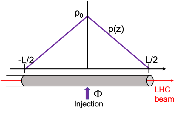
Sketch of a tubular storage cell of length $L$ and inner diameter $D$. Gas is injected at the centre with flow rate $\Phi$, giving a triangular density distribution $\rho (z)$ with maximum $\rho_0$ at the centre. |
PrincS[..].png [69 KiB] HiDef png [57 KiB] Thumbnail [30 KiB] |
|
|
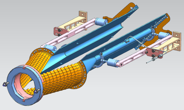
Left: view of the storage cell (blue) supported from the {\gls*{velo}} RF box flanges (in green) in the closed {\gls*{velo}} position. Two flexible wakefield suppressors (orange) provide the electrical continuity. Right: storage cell in the open position (without showing {\gls*{velo}} elements). |
overal[..].png [230 KiB] HiDef png [890 KiB] Thumbnail [262 KiB] |
|
|
cell_o[..].png [214 KiB] HiDef png [596 KiB] Thumbnail [172 KiB] |
|
|
|
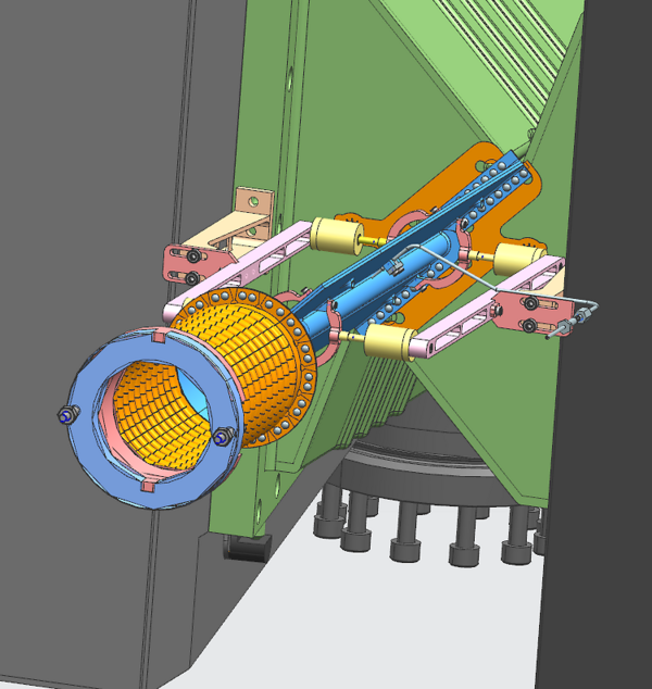
Picture of the {\gls*{smog}} storage cell system installed into the {\gls*{velo}} vessel. |
photo-[..].jpg [956 KiB] HiDef png [2 MiB] Thumbnail [414 KiB] |

|
|
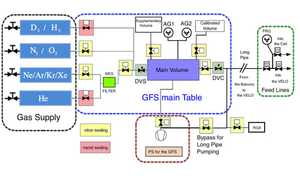
The four assembly groups of the {\gls*{smog}} {\gls*{gfs}} are the gas supply (with 4 reservoirs), the main table, the pumping station (PS) and the feed lines to the {\gls*{velo}} vacuum vessel. The various components are described in the text. |
2018_1[..].png [271 KiB] HiDef png [309 KiB] Thumbnail [114 KiB] |
|
|
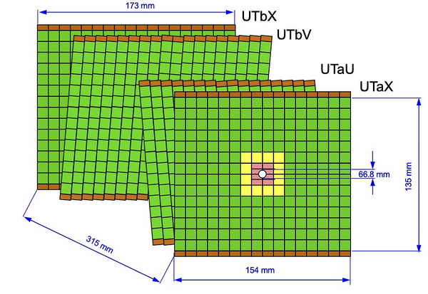
Drawing of the four {\gls*{ut}} silicon planes with indicative dimensions. Different colours designate different types of sensors: Type-A (green), Type-B (yellow), Type-C and Type-D (pink), as described in the text. |
UT_planes.jpg [131 KiB] HiDef png [997 KiB] Thumbnail [227 KiB] |
|
|
A 3D view of the {\gls*{ut}} system. |
ut_gen[..].pdf [1 MiB] HiDef png [2 MiB] Thumbnail [711 KiB] |
|
|
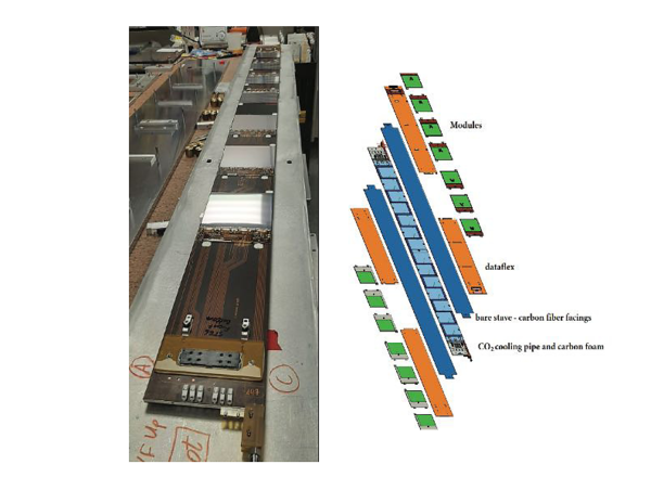
Left: a completed stave. At the bottom, the end of the cooling tube is visible with the high voltage and signal connections. In orange are the dataflex cables and in brown the hybrids. The reflective areas are the silicon detectors. Right: an exploded view of an instrumented stave showing the individual components described in the text. |
stave-[..].pdf [1 MiB] HiDef png [2 MiB] Thumbnail [614 KiB] |
|
|
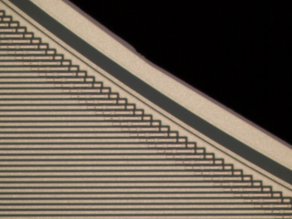
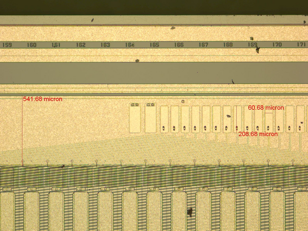
Design features of the {\gls*{ut}} silicon sensors (see text). Left: Type-D sensor cut-out region. Right: Embedded pitch adapter. |
typed_[..].jpg [75 KiB] HiDef png [1 MiB] Thumbnail [288 KiB] |
|
|
pa_photo.jpg [287 KiB] HiDef png [2 MiB] Thumbnail [459 KiB] |
|
|
|
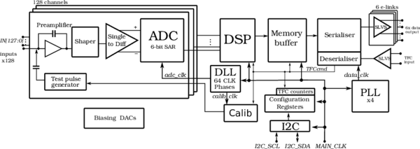
Block diagram of the 128-channel {\gls*{salt}} {\gls*{asic}} . |
salt_block.pdf [40 KiB] HiDef png [110 KiB] Thumbnail [49 KiB] |
|
|
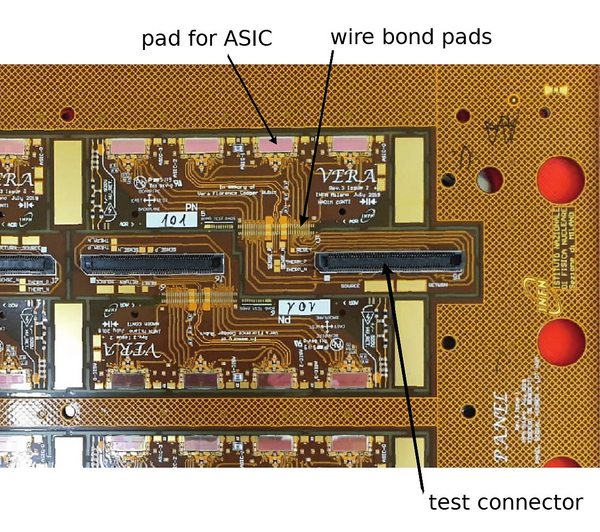
Left: Two fully visible VERA hybrids, not yet equipped with {\gls*{asic}} {s}, embedded in a carrier 8-hybrid panel before cutting. Right: SUSI hybrid mounted in a final {\gls*{ut}} Type-D module. |
veraHybrid.jpg [521 KiB] HiDef png [2 MiB] Thumbnail [585 KiB] |
|
|
module[..].jpg [198 KiB] HiDef png [1 MiB] Thumbnail [315 KiB] |

|
|
|
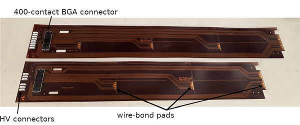
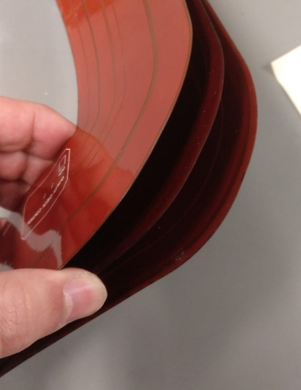
Picture of one Short and one Medium dataflex cable. |
Flex1.jpg [141 KiB] HiDef png [623 KiB] Thumbnail [146 KiB] |
|
|
Left: pigtails in two different shapes; middle: pigtail section showing the 3 subcables; right: installed pigtails. |
pigtails.jpg [1 MiB] HiDef png [2 MiB] Thumbnail [405 KiB] |

|
|
ptribbons.jpg [76 KiB] HiDef png [1 MiB] Thumbnail [296 KiB] |
|
|
|
instal[..].jpg [156 KiB] HiDef png [1 MiB] Thumbnail [294 KiB] |

|
|
|
Schematic of LV, HV, data, fast and slow control signal distribution to {\gls*{ut}} {\gls*{fend}} electronics. |
Data_C[..].jpg [610 KiB] HiDef png [683 KiB] Thumbnail [216 KiB] |

|
|
Left: Illustration of the usage of dataflex cables on the different stave variants. Short cable shaded in blue, Medium in orange and Long in red. The modules hosted by the cable are highlighted with a coloured contour. The numbers 3, 4, 5 indicated the number of wire-bonded e-ports per chip on the given module. Right: Arrangement of a single plane of the {\gls*{ut}} hybrids into power groups sharing a common {\gls*{lv}} output channel. Only one quadrant of the plane is shown. Boxes represent hybrids and the numbers (1 to 4) the power group. |
Flex2.jpg [267 KiB] HiDef png [1 MiB] Thumbnail [436 KiB] |

|
|
hybrid[..].jpg [54 KiB] HiDef png [544 KiB] Thumbnail [132 KiB] |

|
|
|
Simulation of the thermal behaviour of a central stave (variant C) at an inlet $\mathrm{ CO_2}$ temperature of \SI{-25}{ $ ^\circ$ {\text{C}} }. |
utcooling1.jpg [398 KiB] HiDef png [277 KiB] Thumbnail [79 KiB] |

|
|
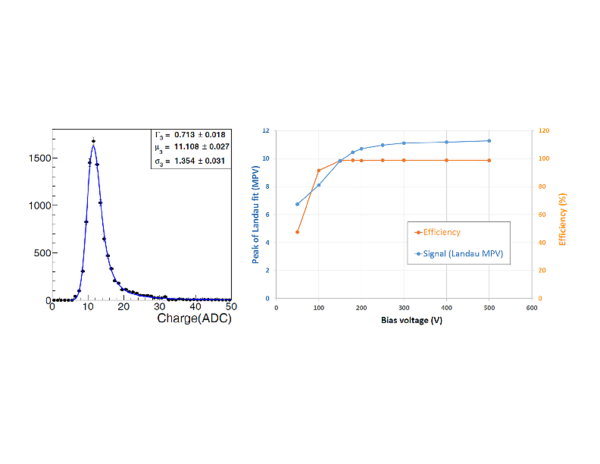
Test beam results for a Type-A unirradiated sensor for tracks with normal incidence. Left: Distribution of collected charge (in ADC counts) at 300 $\text{ V}$ bias. The data are fitted with a Landau distribution convoluted with a Gaussian function. Right: Most probable value of the Landau fit result and hit efficiency versus the applied bias voltage. |
Fermil[..].pdf [216 KiB] HiDef png [377 KiB] Thumbnail [110 KiB] |
|
|
The raw and common mode subtracted noise measured in a single hybrid with only that hybrid powered and configured (blue and red curves, respectively) compared with the noise measured in the same hybrid when all hybrids in the stave were operating (black and cyan). |
ut_sli[..].pdf [31 KiB] HiDef png [395 KiB] Thumbnail [277 KiB] |

|
|
Material scan through the {\gls*{ut}} detector, with thickness given as a fraction of a radiation length. Left: thickness map in $xy$ plane for normal track incidence. Right: thickness as a function of pseudorapidity ($\eta$) as seen from the interaction point. |
matthi[..].pdf [17 KiB] HiDef png [84 KiB] Thumbnail [42 KiB] |

|
|
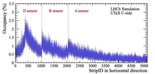
Expected {\gls*{ut}} strip occupancies for minimum bias events in the sensors near the detector midline ($y=0$). |
ut_occ[..].jpg [123 KiB] HiDef png [387 KiB] Thumbnail [117 KiB] |
|
|
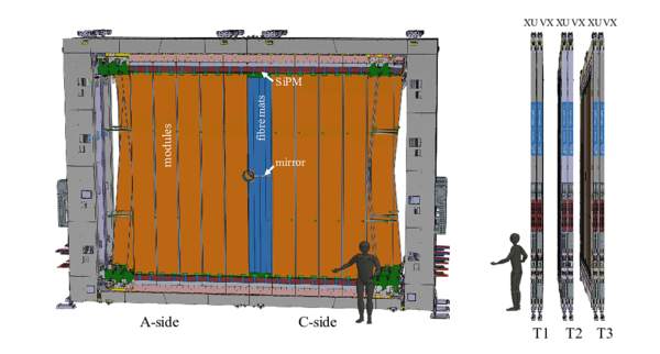
Front and side views of the 3D model of the {\gls*{sft}} detector. |
3stati[..].pdf [255 KiB] HiDef png [1 MiB] Thumbnail [469 KiB] |
|
|
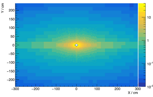
Map of the total expected ionising dose in $\text{ kGy}$ for an integrated luminosity of 50 $\text{ fb} ^{-1}$ at the T1 station of the {\gls*{sft}} from Fluka simulations of the LHCb detector. |
dosemap_T1.jpg [173 KiB] HiDef png [204 KiB] Thumbnail [74 KiB] |
|
|
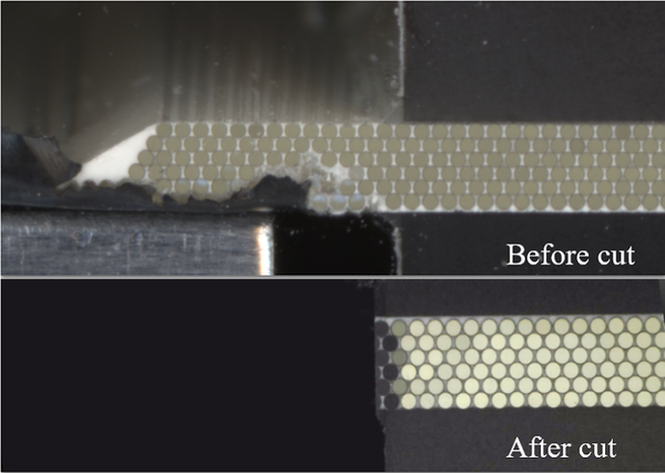
Left: view of a fibre mat with a microscope before and after the side fibres are cut away. Right: a photo of a fibre mat with the polycarbonate end-pieces and {\gls*{sipm}} alignment holes. Figures from Ref. [84]. |
fibree[..].jpg [279 KiB] HiDef png [1 MiB] Thumbnail [268 KiB] |
|
|
fibremat.jpg [160 KiB] HiDef png [1 MiB] Thumbnail [276 KiB] |

|
|
|
A cross-section and projections with dimensions (in $\text{ mm}$ ) of a scintillating fibre module and its components. The outlines of the fibre mats and light injection system (LIS) are shown with dashed lines. The nominal gap between fibre mats is shown in a zoomed inset on the left. |
SCIFI-[..].jpg [142 KiB] HiDef png [441 KiB] Thumbnail [127 KiB] |

|
|
The traversed amount of material, averaged over azimuthal angle $\phi$, in units of (left) hadronic interaction length and (right) radiation length as a function of $\eta$ for a sample of simulated $ B ^0_ s \rightarrow \phi\phi$ decays. The total average is also shown for $\eta$ between 2.2 and 4.5 (range limited to the acceptance of the {\gls*{sft}} shown with dashed lines) |
radlen[..].pdf [56 KiB] HiDef png [63 KiB] Thumbnail [31 KiB] |

|
|
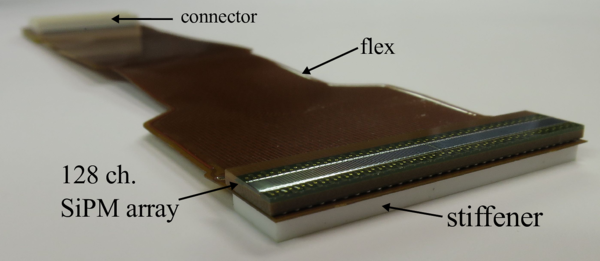
An H2017 {\gls*{sipm}} array bonded to a flex cable. The white stiffener is visible on the lower side of the flex cable. |
h2017_[..].pdf [214 KiB] HiDef png [3 MiB] Thumbnail [703 KiB] |
|
|
Left: correlated noise probabilities for an H2017 detector as a function of $\rm \Delta V$ . Right: dark-count rate for an irradiated {\gls*{sipm}} as a function of temperature for three overvoltages. |
dcr_6e11.pdf [24 KiB] HiDef png [375 KiB] Thumbnail [321 KiB] |

|
|
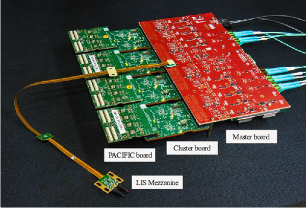
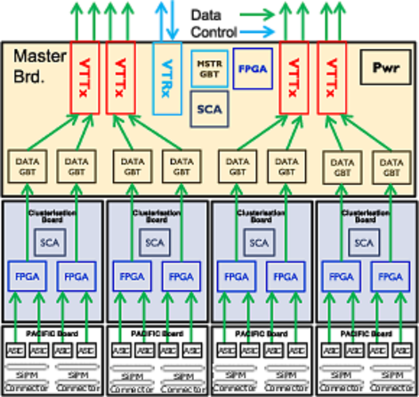
Left: picture of assembled Master, Clusterisation and PACIFIC boards. Right: corresponding schematics of signal data routing. |
HALFROB.pdf [110 KiB] HiDef png [5 MiB] Thumbnail [1 MiB] |
|
|
BlockS[..].pdf [86 KiB] HiDef png [833 KiB] Thumbnail [760 KiB] |
|
|
|
PACIFICr5q Channel block diagram. |
pacifi[..].pdf [31 KiB] HiDef png [57 KiB] Thumbnail [27 KiB] |

|
|
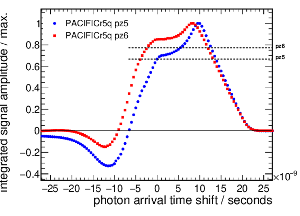
Left: the simulated shaper amplitude as a function of time for a single 10 photoelectron signal at \SI{4}{ $\text{ V}$ } above breakdown. Right: the track-and-hold output values as a function of signal arrival time. The dashed lines indicate the nominal threshold value with respect to the maximum value for two settings (pz5 and pz6, see text). |
shaper[..].pdf [15 KiB] HiDef png [168 KiB] Thumbnail [144 KiB] |

|
|
p5q_pz[..].pdf [19 KiB] HiDef png [206 KiB] Thumbnail [201 KiB] |
|
|
|
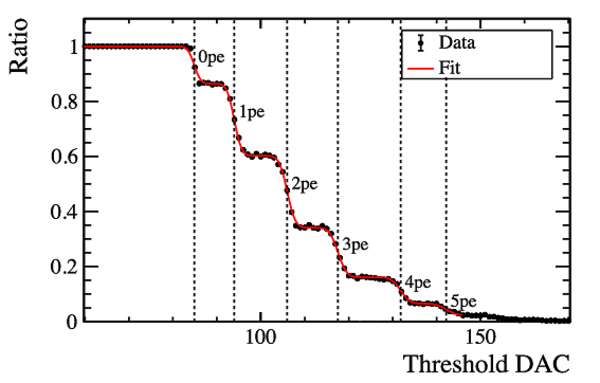
Left: an example threshold calibration for one comparator of one channel, showing the ratio (number of data above threshold to the total number of data) as a function of the threshold value. The red curve is the result of a fit. The vertical dashed lines through the steps highlight the discrete photoelectron amplitudes. Right: a diagram of the clustering algorithm. |
ScurveFit.pdf [39 KiB] HiDef png [152 KiB] Thumbnail [154 KiB] |
|
|
cluste[..].pdf [26 KiB] HiDef png [149 KiB] Thumbnail [127 KiB] |

|
|
|
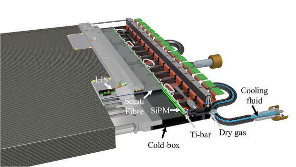
A cutaway view of the cold-box fixed to the fibre module. |
coldbox.pdf [201 KiB] HiDef png [2 MiB] Thumbnail [622 KiB] |
|
|
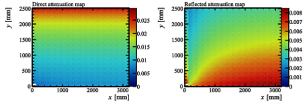
The survival probability (attenuation) map of direct and reflected photons in the {\gls*{sft}} after 50 $\text{ fb} ^{-1}$ from simulation. |
attenmap.pdf [239 KiB] HiDef png [1 MiB] Thumbnail [398 KiB] |
|
|
Simulated number of thermal-noise clusters per 25 $\text{ ns}$ clock cycle as a function of the {\gls*{dcr}} . The curves stem from a power law fit to the data points. The comparison is made for two different models of the PACIFIC settings (in blue the pz5 settings, in red the pz6). The three threshold values used are 1.5, 2.5 and 4.5 photoelectrons. |
toy_fi[..].pdf [40 KiB] HiDef png [145 KiB] Thumbnail [89 KiB] |

|
|
Left: the single hit inefficiency of the five most efficient fine time bins of all channels measured at several positions across the module. The distribution is fit to a log-normal distribution. The mean and standard deviation of the log-normal distribution is also shown. Right: an example hit position residual distribution fitted with a single (dashed curve) and double (solid curve) Gaussian function. Gap regions have been excluded. |
hondie_5ns.pdf [58 KiB] HiDef png [56 KiB] Thumbnail [27 KiB] |

|
|
double[..].pdf [21 KiB] HiDef png [454 KiB] Thumbnail [417 KiB] |
|
|
|
Schematic view of the (left) RICH1 and (right) RICH2 detectors. |
rich1l[..].jpg [341 KiB] HiDef png [3 MiB] Thumbnail [887 KiB] |

|
|
rich2l[..].jpg [881 KiB] HiDef png [1 MiB] Thumbnail [386 KiB] |
|
|
|
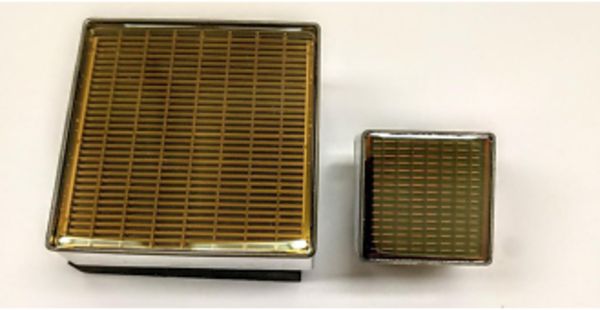
Left: the {\gls*{mapmt}} {s} selected for the upgraded RICH detectors with the 2-inch model on the left and the 1-inch model on the right. Right: scheme of the internal structure of the {\gls*{mapmt}} {}. |
MaPMTs.pdf [192 KiB] HiDef png [3 MiB] Thumbnail [839 KiB] |
|
|
multia[..].jpg [235 KiB] HiDef png [368 KiB] Thumbnail [113 KiB] |

|
|
|
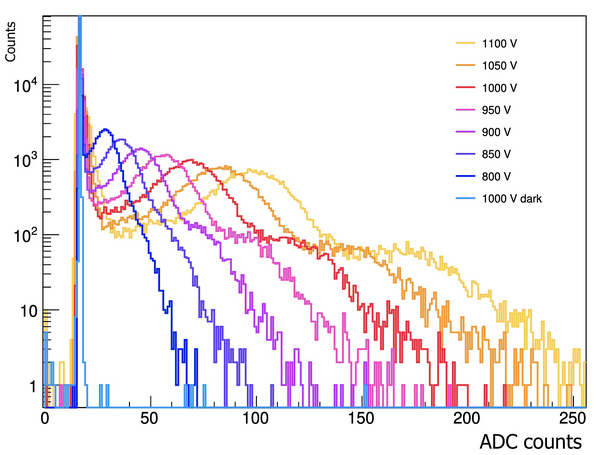
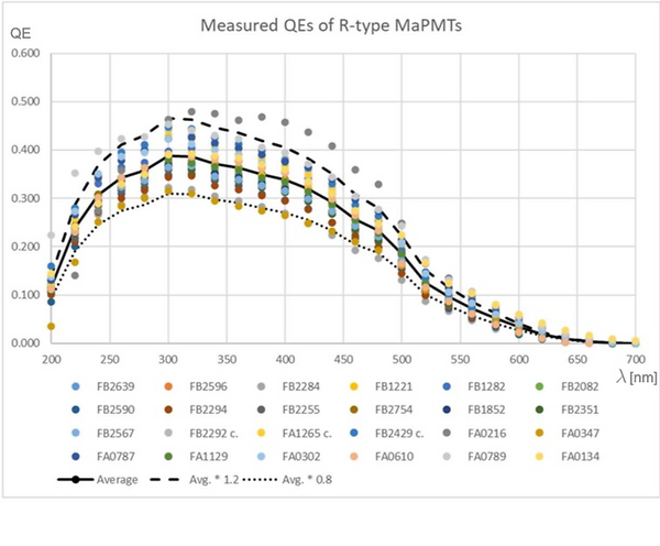
Left: typical signal amplitude spectra for a pixel as a function of the {\gls*{hv}} value. Right: {\gls*{qe}} curves for a batch of 1-inch {\gls*{mapmt}} {s} from the production: the ultra bi-alkali photocathode allows to reach excellent {\gls*{qe}} values. |
MaPMTs[..].jpg [345 KiB] HiDef png [399 KiB] Thumbnail [113 KiB] |
|
|
MaPMT_[..].jpg [85 KiB] HiDef png [464 KiB] Thumbnail [141 KiB] |
|
|
|
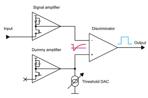
Left: CLARO {\gls*{asic}} with its packaging. Right: block schematic of a CLARO channel. The purpose of the dummy amplifier is to give each channel a differential structure, improving the power supply rejection ratio and allowing DC-coupled input to the discriminator. |
claroChip.jpg [329 KiB] HiDef png [2 MiB] Thumbnail [515 KiB] |

|
|
claroS[..].jpg [104 KiB] HiDef png [148 KiB] Thumbnail [47 KiB] |
|
|
|
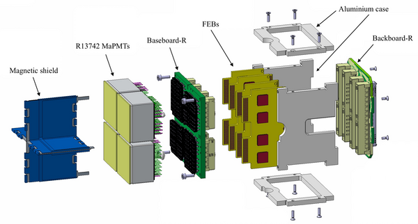
Exploded view of the {\gls*{ecr}} . |
ECRexp[..].jpg [497 KiB] HiDef png [347 KiB] Thumbnail [105 KiB] |
|
|
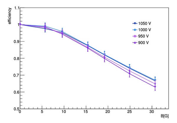
Counting efficiency as a function of the longitudinal magnetic field for an edge pixel, at different values of {\gls*{hv}} , for an {\gls*{ecr}} (left) without and (right) with the magnetic shield. |
withoutMS.jpg [90 KiB] HiDef png [177 KiB] Thumbnail [58 KiB] |
|
|
withMS.jpg [81 KiB] HiDef png [160 KiB] Thumbnail [51 KiB] |

|
|
|
Schematic view of the {\gls*{ech}} |
ECHexp[..].jpg [241 KiB] HiDef png [267 KiB] Thumbnail [78 KiB] |

|
|
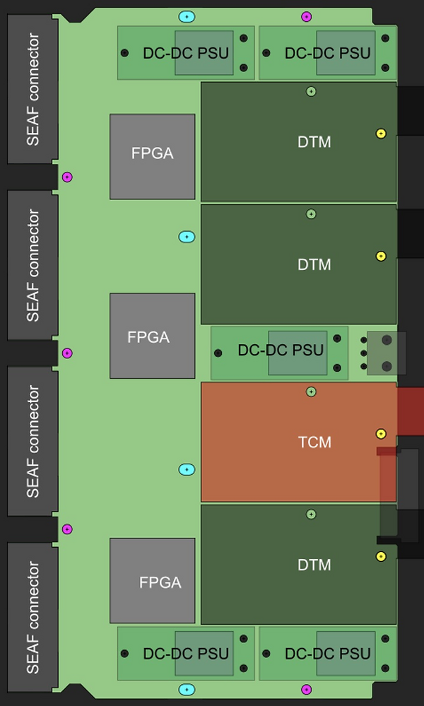
Left: picture of a fully populated {\gls*{pdmdb}} -R board. Right: schematic view of the {\gls*{pdmdb}} -R board main components. The {\gls*{pdmdb}} -H differs by having one less {\gls*{fpga}} and {\gls*{dtm}} with respect to the {\gls*{pdmdb}} -R. |
pdmdbr.jpg [499 KiB] HiDef png [2 MiB] Thumbnail [694 KiB] |

|
|
pdmdbr[..].jpg [115 KiB] HiDef png [719 KiB] Thumbnail [187 KiB] |
|
|
|
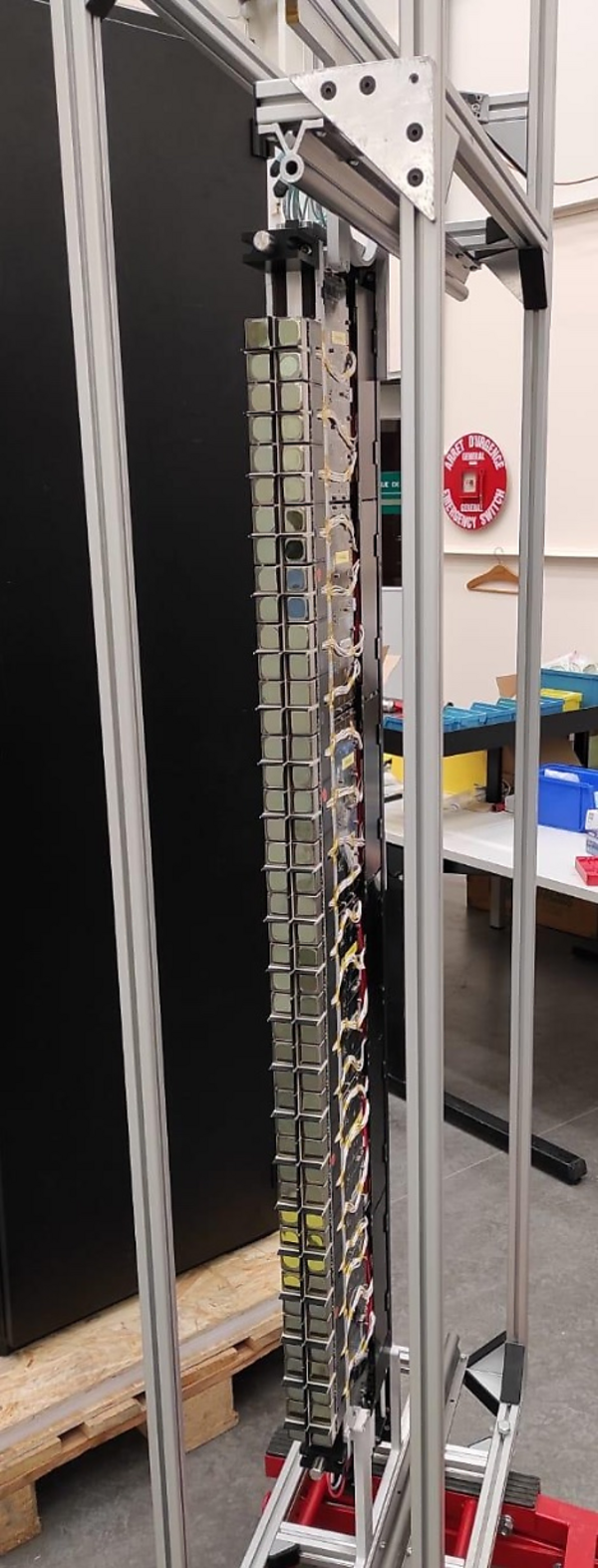
Pictures of (left) a completed RICH1 column (front view) and (right) a RICH2 column (side view, {\gls*{ec}} {s} on the left), with the photon detector chain and the complete set of services. |
R1col.jpg [186 KiB] HiDef png [4 MiB] Thumbnail [930 KiB] |
|
|
202007[..].jpg [811 KiB] HiDef png [4 MiB] Thumbnail [952 KiB] |

|
|
|
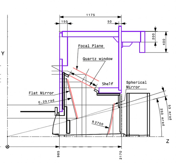
The optical geometries of (left) the original and (right) the upgraded RICH1 . |
RICH1-[..].jpg [95 KiB] HiDef png [367 KiB] Thumbnail [115 KiB] |
|
|
RICH1-[..].jpg [99 KiB] HiDef png [371 KiB] Thumbnail [122 KiB] |

|
|
|
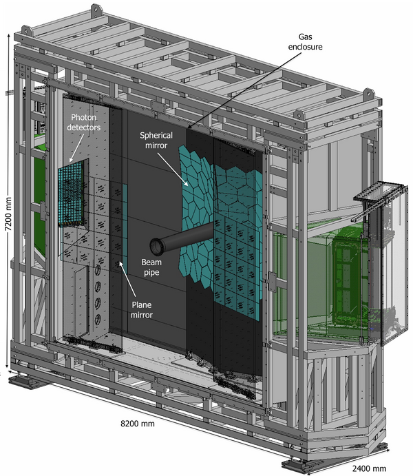
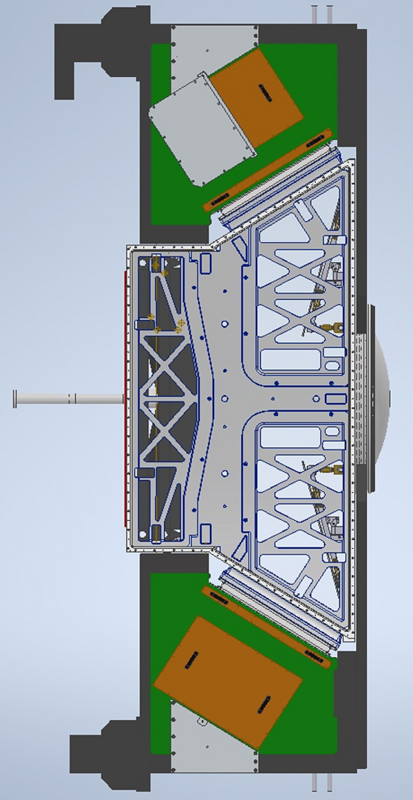
Left: Side view CAD layout of the RICH1 gas enclosure. Right: photo of the RICH1 gas enclosure after its installation in the LHCb cavern. |
gas-en[..].jpg [155 KiB] HiDef png [2 MiB] Thumbnail [512 KiB] |
|
|
gasEnc[..].jpg [543 KiB] HiDef png [3 MiB] Thumbnail [754 KiB] |
|
|
|
Pictures of (left) the spherical and (right) the bottom flat mirror assemblies. |
rich1s[..].jpg [51 KiB] HiDef png [1 MiB] Thumbnail [326 KiB] |
|
|
rich1flat.jpg [169 KiB] HiDef png [2 MiB] Thumbnail [584 KiB] |

|
|
|
Picture of RICH1 columns while being inserted into their support structure, the lower {\gls*{mapmt}} {} chassis. The rails and alignment structures are visible on the left side. The chassis is mounted to the soft-iron magnetic shielding that surrounds the {\gls*{mapmt}} {} region. The push connector for the copper-carried services is visible as well in the left-most column. |
rich1box.jpg [301 KiB] HiDef png [2 MiB] Thumbnail [483 KiB] |

|
|
Fully assembled and commissioned RICH2 photon detector array. Left: CAD view; right: photograph taken in the assembly area |
RICH2-[..].jpg [404 KiB] HiDef png [2 MiB] Thumbnail [542 KiB] |

|
|
rich2_[..].jpg [159 KiB] HiDef png [3 MiB] Thumbnail [651 KiB] |

|
|
|
RICH2 photon detection system inside its enclosure. Left: CAD view; right: photograph |
RICH2-[..].jpg [417 KiB] HiDef png [1 MiB] Thumbnail [463 KiB] |
|
|
RICH2-[..].jpg [1 MiB] HiDef png [5 MiB] Thumbnail [998 KiB] |
|
|
|
Typical output of the DAC scans procedure. On the left, the calibration of a single CLARO channel with offset bit enabled and no attenuation is shown. The charge (in units of electron charge) corresponding to a threshold DAC code (th) is determined by the linear relation $Q=Q_0 + Q_\text{th}\cdot\text{th}$. On the right, the distribution of the charges (in units of electron charge) corresponding to one threshold step ($Q_\text{th}$) for a RICH2 column is shown. The linearity of the threshold setting as a function of the injected charge is found to be excellent for all attenuation and offset values. |
single[..].jpg [222 KiB] HiDef png [172 KiB] Thumbnail [72 KiB] |

|
|
thresh[..].jpg [199 KiB] HiDef png [340 KiB] Thumbnail [99 KiB] |

|
|
|
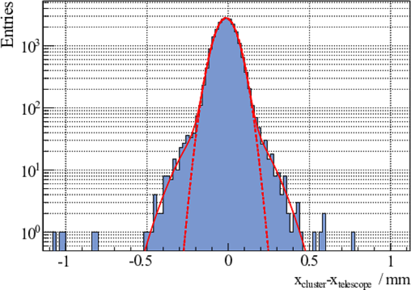
Left: distribution of RICH2 thresholds of the CLARO comparator converted into absolute charge (black). The mean and standard deviations of the distribution are $(207.58 \pm 0.16)\times 10^3$ electrons and $(39.64 \pm 0.10)\times 10^3$ electrons. The threshold settings can be compared to the pixel gain at 900 $\text{ V}$ (red), 950 $\text{ V}$ (green) and 1000 $\text{ V}$ (blue). Right: RICH1 simulated photon detector hit time distribution showing the signal peak (S) and a possible time gate in the front-end electronics. |
rich2w[..].pdf [17 KiB] HiDef png [145 KiB] Thumbnail [129 KiB] |

|
|
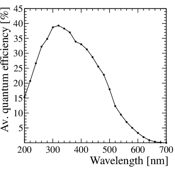
Left: average quantum efficiency of the {\gls*{mapmt}} {s} used in the RICH detectors. Right: a typical {\gls*{pid}} performance of the kaon identification obtained from the LHCb software for the configuration described in the text (red). A corresponding curve for the Run 2 conditions (prepared using the simulation with LHCb Run 2 geometry and luminosity, as reported in Ref. [118]) is shown for reference (black). |
qeAverage.pdf [14 KiB] HiDef png [134 KiB] Thumbnail [81 KiB] |
|
|
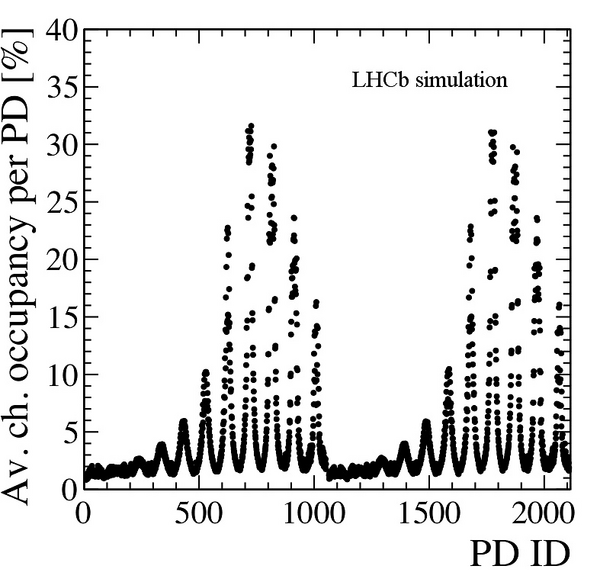
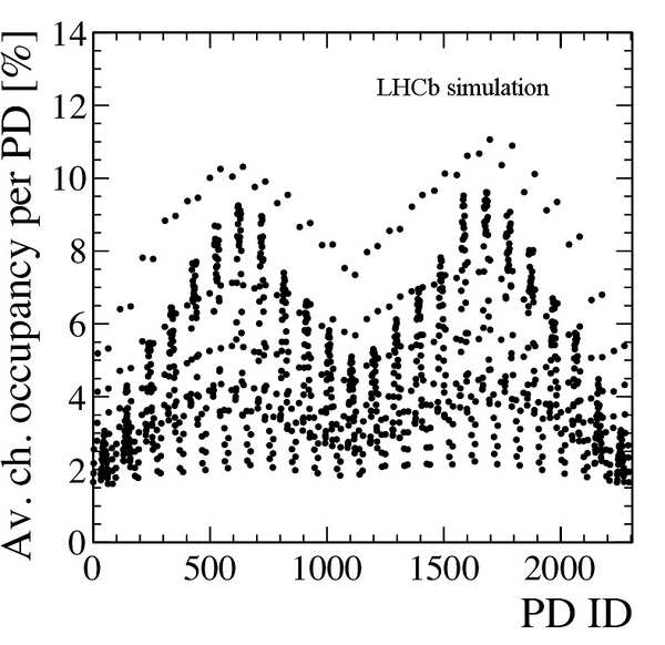
Average expected occupancy per channel for different {\gls*{mapmt}} {s} in the (left) RICH1 and (right) RICH2 detector. |
occupa[..].jpg [128 KiB] HiDef png [200 KiB] Thumbnail [63 KiB] |
|
|
occupa[..].jpg [161 KiB] HiDef png [243 KiB] Thumbnail [77 KiB] |
|
|
|
Lateral segmentation of (left) the {\gls*{ecal}} and (right) the {\gls*{hcal}} . One quarter of the detector front face is shown. |
Calo_s[..].png [178 KiB] HiDef png [108 KiB] Thumbnail [64 KiB] |

|
|
Schematic of an {\gls*{ecal}} cell. |
Calo_E[..].jpg [271 KiB] HiDef png [498 KiB] Thumbnail [159 KiB] |

|
|
Schematic of an {\gls*{hcal}} cell. |
Calo_H[..].jpg [237 KiB] HiDef png [518 KiB] Thumbnail [148 KiB] |
|
|
Picture of the {\gls*{feb}} . |
Calo_F[..].jpg [245 KiB] HiDef png [2 MiB] Thumbnail [538 KiB] |

|
|
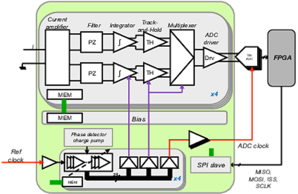
Block diagram of the ICECAL {\gls*{asic}} . |
ICECAL[..].pdf [54 KiB] HiDef png [301 KiB] Thumbnail [284 KiB] |
|
|
Schematic of the calorimeter crate. |
Calo_crate.png [194 KiB] HiDef png [184 KiB] Thumbnail [90 KiB] |

|
|
Control board connection scheme with the new {\gls*{gbt}} {} protocol. |
DCS_GBT.jpg [262 KiB] HiDef png [82 KiB] Thumbnail [33 KiB] |

|
|
{\gls*{feb}} test beam results. Left: integrated charge (ADC counts) as a function of hit time phase with respect to the internal 40 $\text{ MHz}$ clock. Right: spillover measured in different clock cycles as a function of the beam energy. |
Calo_T[..].pdf [80 KiB] HiDef png [502 KiB] Thumbnail [267 KiB] |

|
|
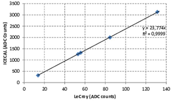
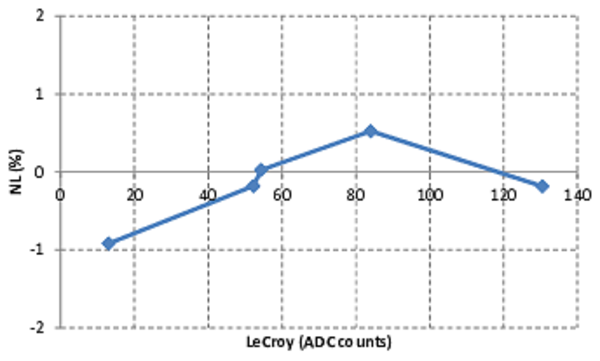
Left: energy values measured with the {\gls*{feb}} prototype at a beam test with respect to the reference charge integrator values. Right: the nonlinearity deviation is shown to be less than 1%. |
Calo_T[..].pdf [77 KiB] HiDef png [194 KiB] Thumbnail [261 KiB] |
|
|
Calo_TB_NL.pdf [77 KiB] HiDef png [165 KiB] Thumbnail [203 KiB] |
|
|
|
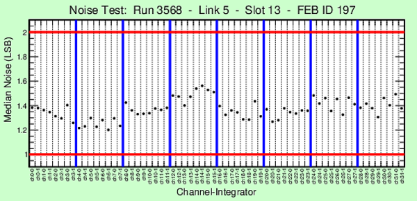
Noise of all channels of a {\gls*{feb}} , measured in laboratory conditions. |
Calo_noise.pdf [58 KiB] HiDef png [530 KiB] Thumbnail [438 KiB] |
|
|
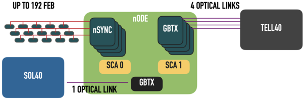
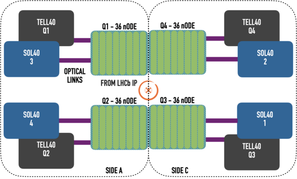
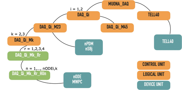
{\gls*{node}} communication scheme. |
nOde_s[..].png [85 KiB] HiDef png [70 KiB] Thumbnail [37 KiB] |
|
|
nOde_s[..].png [275 KiB] HiDef png [192 KiB] Thumbnail [90 KiB] |
|
|
|
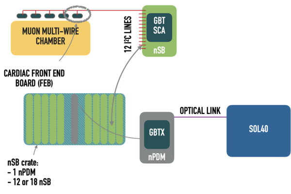
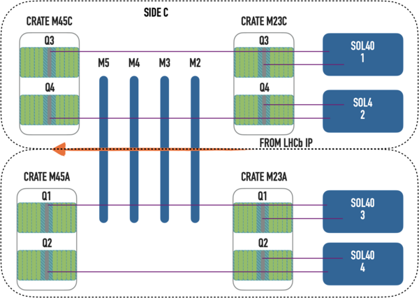
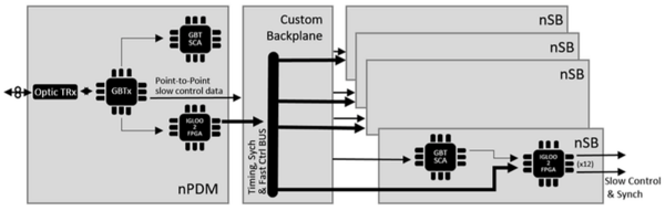
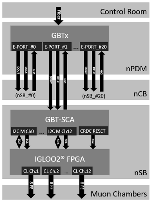
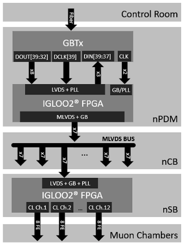
{\gls*{fend}} electronics communication scheme. |
nSB_scheme.png [201 KiB] HiDef png [143 KiB] Thumbnail [68 KiB] |
|
|
nSB_sc[..].png [271 KiB] HiDef png [227 KiB] Thumbnail [102 KiB] |
|
|
|
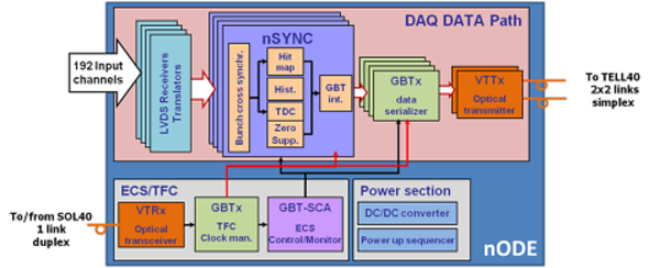
{\gls*{node}} block diagram |
nODE_BD.pdf [112 KiB] HiDef png [946 KiB] Thumbnail [261 KiB] |
|
|
{\gls*{node}} board layout |
nODE_L[..].png [167 KiB] HiDef png [721 KiB] Thumbnail [235 KiB] |

|
|
Schematic view of the {\gls*{nsync}} architecture and its interface with the GBT chipset [139]. |
nSYNCd[..].png [244 KiB] HiDef png [494 KiB] Thumbnail [140 KiB] |

|
|
{\gls*{nsbs}} block diagram |
nSBS_BD.png [60 KiB] HiDef png [109 KiB] Thumbnail [42 KiB] |
|
|
Left: functional representation of the {\gls*{nsbs}} {\gls*{ecs}} path. Right: functional representation of the {\gls*{nsbs}} {\gls*{tfc}} path |
nSBS_ECS.png [43 KiB] HiDef png [318 KiB] Thumbnail [125 KiB] |
|
|
nSBS_TFC.png [41 KiB] HiDef png [306 KiB] Thumbnail [121 KiB] |
|
|
|
Finite state machine hierarchy scheme (example for the Side A ). |
nFSM.jpg [237 KiB] HiDef png [275 KiB] Thumbnail [90 KiB] |
|
|
Mechanical drawing of the tungsten shielding around the beam pipe. |
tungst[..].jpg [274 KiB] HiDef png [1018 KiB] Thumbnail [231 KiB] |
|
|
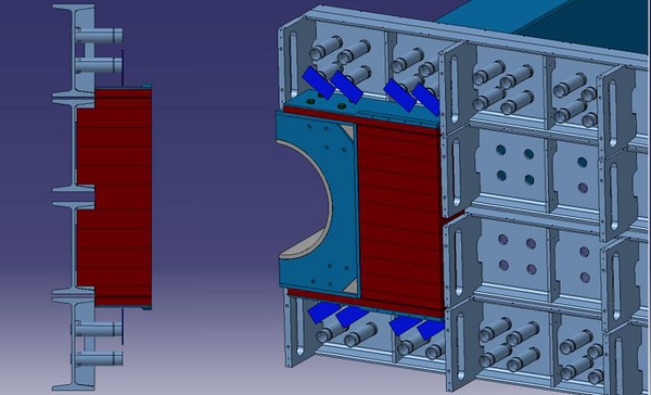
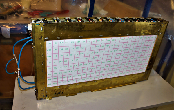
Left: M2R2 new pad chamber prototype. Right: M2R1 new pad chamber prototype. |
M2R2.jpg [1013 KiB] HiDef png [1 MiB] Thumbnail [352 KiB] |
|
|
M2R1.jpg [1006 KiB] HiDef png [1 MiB] Thumbnail [355 KiB] |

|
|
|
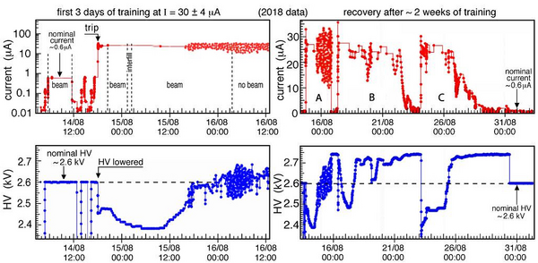
Typical recovery procedure for a gap (data are from a chamber in region M5R3). The plots on the left show (top) the current and (bottom) the {\gls*{hv}} setting during a period of about three days around the first appearance of the {\gls*{hv}} trip and the subsequent start of {\gls*{hv}} training. The plots on the right show (top) the current and (bottom) the {\gls*{hv}} setting during the full recovery procedure, which lasted about two weeks. The nominal {\gls*{hv}} setting for this gap is 2600 $\text{ V}$ . in normal conditions, the average current in presence of colliding beams is about 0.6 $\text{ \muA}$ . |
MWPC_L[..].jpg [372 KiB] HiDef png [586 KiB] Thumbnail [173 KiB] |
|
|
Current in the {\gls*{mwpc}} during the Malter-effect recovery training: default mixture (full circles) is compared with a mixture containing $\sim$2% of oxygen (open circles). |
MWPC_L[..].png [78 KiB] HiDef png [192 KiB] Thumbnail [84 KiB] |

|
|
Upgraded LHCb online system. All system components are connected to the {\gls*{ecs}} shown on the right, although these connections are not shown in the figure for clarity. |
lhcb-o[..].png [272 KiB] HiDef png [305 KiB] Thumbnail [138 KiB] |

|
|
View of the {\gls*{pciefty}} board. |
PCIe40[..].png [422 KiB] HiDef png [1009 KiB] Thumbnail [217 KiB] |

|
|
{\gls*{tellfty}} firmware architecture. Common blocks in blue; specific subdetector blocks in red. |
TELL40[..].png [156 KiB] HiDef png [210 KiB] Thumbnail [101 KiB] |

|
|
Logical architecture of the upgrade {\gls*{tfc}} system. |
TFClog[..].PNG [77 KiB] HiDef png [231 KiB] Thumbnail [92 KiB] |
|
|
Schematic view of the packing mechanism to merge {\gls*{tfc}} and {\gls*{ecs}} information on the same {\gls*{gbt}} links towards the {\gls*{fend}} electronics. {\gls*{gbt}} words are subdivided into small e-links. |
[Failure to get the plot] | |
|
Scope of the {\gls*{ecs}} . |
ecs-global.png [149 KiB] HiDef png [175 KiB] Thumbnail [78 KiB] |

|
|
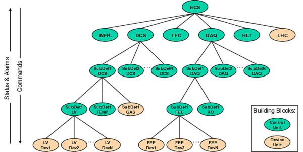
Simplified {\gls*{ecs}} architecture. |
ecs-arch.pdf [41 KiB] HiDef png [351 KiB] Thumbnail [195 KiB] |
|
|
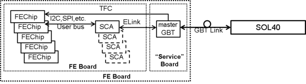
{ {\gls*{fend}} }- {\gls*{ecs}} interface |
fe-ecs.png [12 KiB] HiDef png [42 KiB] Thumbnail [22 KiB] |
|
|
LHCb Run Control panel. |
RunCon[..].jpg [736 KiB] HiDef png [874 KiB] Thumbnail [251 KiB] |

|
|
Aggregated data-rate in the LHCb event-builder network as a function of the number of builder units for various nominal event-fragment sizes. |
eb_sca[..].png [45 KiB] HiDef png [169 KiB] Thumbnail [59 KiB] |

|
|
Online data flow [171]. |
RTA_da[..].pdf [25 KiB] HiDef png [293 KiB] Thumbnail [153 KiB] |

|
|
Baseline {\gls*{hltone}} sequence, updated from [177]. Rhombi represent algorithms reducing the event rate, while rectangles represent algorithms processing data. |
Fig_109.pdf [34 KiB] HiDef png [46 KiB] Thumbnail [19 KiB] tex code |

|
|
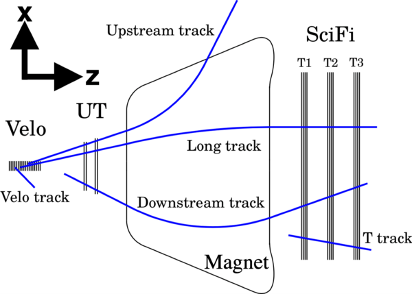
Track types in the LHCb detector bending plane. |
track_[..].png [243 KiB] HiDef png [165 KiB] Thumbnail [69 KiB] |
|
|
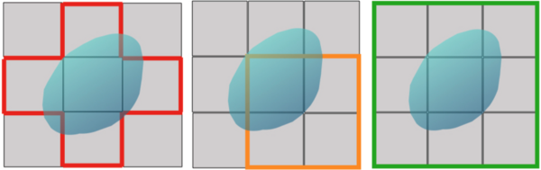
Shapes used for the upgrade calorimeter reconstruction, referred to as cross (left), $\mathit{2\times 2}$ (centre) and $\mathit{3\times 3}$ (right). |
CALO_S[..].png [305 KiB] HiDef png [197 KiB] Thumbnail [39 KiB] |
|
|
Schematic view of the real-time alignment and calibration procedure starting at the beginning of each fill. |
Scheme[..].pdf [15 KiB] HiDef png [277 KiB] Thumbnail [122 KiB] |

|
|
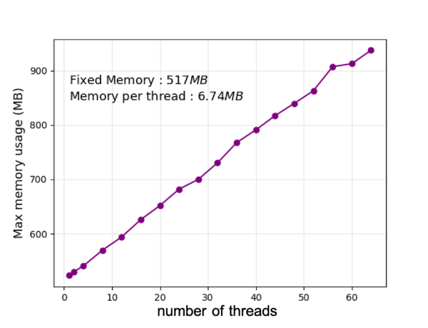
Memory consumption of a prototype {\gls*{hltone}} application when run in (left) multijob and (right) multithread modes. The application was run on 3000 events per thread on a reference server node with 20 physical cores and a factor 2 hyper-threading. Note that the y-axis scale of the right plot does not start at zero. |
MemPlo[..].png [79 KiB] HiDef png [129 KiB] Thumbnail [42 KiB] |

|
|
MemPlo[..].png [86 KiB] HiDef png [140 KiB] Thumbnail [47 KiB] |
|
|
|
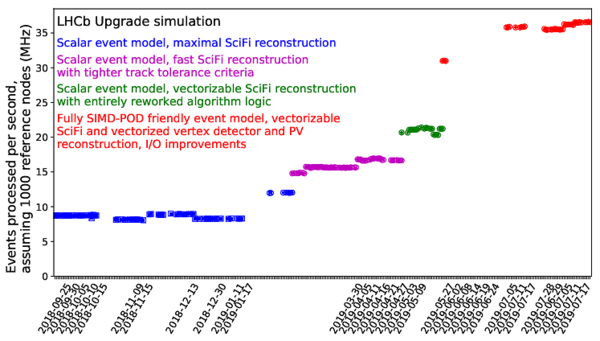
Evolution of the throughput of the CPU-based {\gls*{hltone}} prototype application between autumn 2018 and summer 2019, as measured on a reference server. |
hlt1_e[..].pdf [25 KiB] HiDef png [443 KiB] Thumbnail [271 KiB] |
|
|
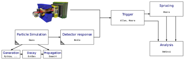
Schematic representation of the LHCb upgrade data flowand the related LHCb application, with an emphasis on simulation. |
lhcb_r[..].pdf [1 MiB] HiDef png [248 KiB] Thumbnail [84 KiB] |
|
|
Schematic structure of the Gauss application. |
Gauss-[..].png [226 KiB] HiDef png [166 KiB] Thumbnail [68 KiB] |

|
|
Graphical representation of the dependencies in the simulation software stack in (left) Run 1-2 and (right) in the upgrade, where the experiment agnostic package Gaussino decouples Gauss from Pythia and Geant4 . |
Gauss-[..].png [110 KiB] HiDef png [212 KiB] Thumbnail [70 KiB] |

|
|
GonG-d[..].png [124 KiB] HiDef png [236 KiB] Thumbnail [84 KiB] |

|
|
|
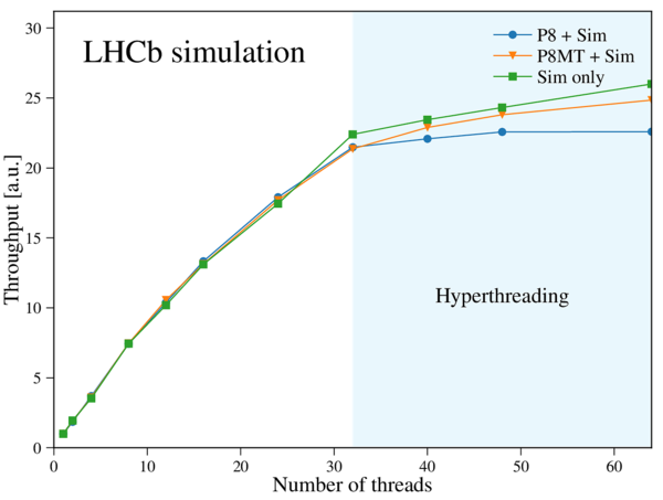
Throughput and memory scaling for the generation of {\gls*{prpr}} collisions producing at least a $ D ^0$ meson with beam conditions as found in the 2016 data-taking period in LHCb. Shown are the curves for a shared (P8) and a thread-local (P8MT) interface to Pythia8 , followed by the Geant4 -based simulation. The contribution of the simulation phase, as obtained by reading the generated events from file ("Sim only"), is also shown. Figure is reproduced from Ref. [217]. |
Throug[..].pdf [51 KiB] HiDef png [243 KiB] Thumbnail [126 KiB] |
|
|
A flow-chart representing the Lamarr project as a pipeline of parametrisations. |
lamarr[..].pdf [14 KiB] HiDef png [43 KiB] Thumbnail [18 KiB] |

|
|
Offline data flow. Figure taken from Ref. [171]. |
DPA_da[..].pdf [34 KiB] HiDef png [316 KiB] Thumbnail [164 KiB] |

|
|
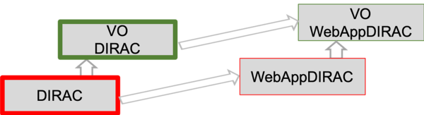
Diagram of a DIRAC release components. The concepts of (top) horizontal and (bottom) vertical extensibility are illustrated. |
DIRAC_[..].png [70 KiB] HiDef png [64 KiB] Thumbnail [37 KiB] |

|
|
DIRAC_[..].png [51 KiB] HiDef png [62 KiB] Thumbnail [34 KiB] |
|
|
|
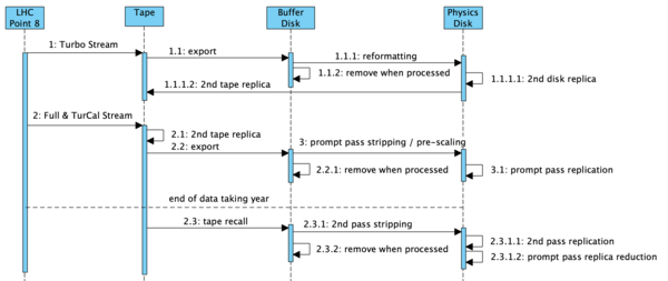
The LHCb offline data processing workflow. |
offlin[..].png [192 KiB] HiDef png [87 KiB] Thumbnail [50 KiB] |
|
|
Throughput of the HLT1 application on a selected subset of current generation {\gls*{gpu}} cards and a representative modern CPU server. |
allen_[..].pdf [21 KiB] Thumbnail [135 KiB] |

|
|
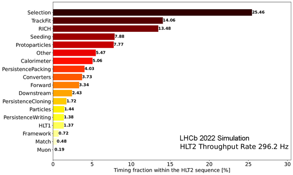
Throughput of the {\gls*{hlttwo}} application and fraction of {\gls*{hlttwo}} resources used by different parts of the reconstruction and selections, measured on a representative {\gls*{hlttwo}} server. A total of 1111 selection algorithms were executed as part of this test. |
HLT2Th[..].jpg [245 KiB] HiDef png [111 KiB] Thumbnail [55 KiB] |
|
|
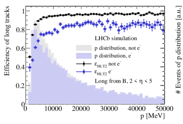
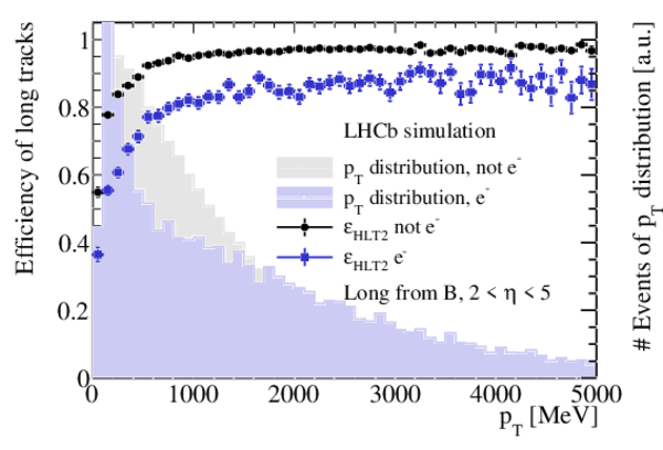
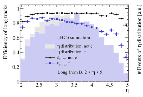
Long track reconstruction efficiency versus momentum $ p$ , transverse momentum $ p_{\mathrm{T}}$ , pseudo-rapidity $\eta$ , and number of primary vertices for long reconstructible electrons (blue squares) and non-electron (black dots) particles from $ B $ decays within $2<\eta <5$. Shaded histograms show the distributions of reconstructible particles. |
BestLo[..].pdf [22 KiB] HiDef png [370 KiB] Thumbnail [273 KiB] |
|
|
BestLo[..].pdf [22 KiB] HiDef png [364 KiB] Thumbnail [267 KiB] |
|
|
|
BestLo[..].pdf [17 KiB] HiDef png [347 KiB] Thumbnail [246 KiB] |
|
|
|
BestLo[..].pdf [16 KiB] HiDef png [250 KiB] Thumbnail [201 KiB] |

|
|
|
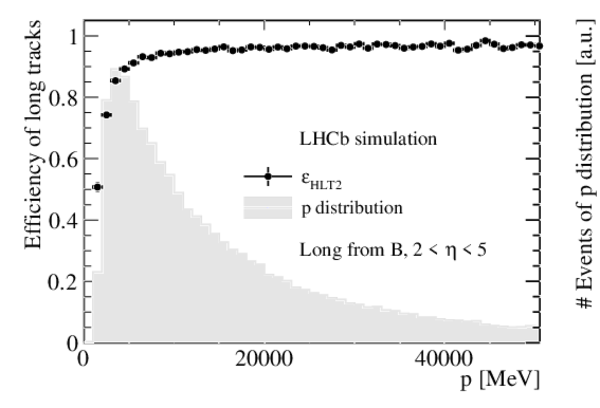
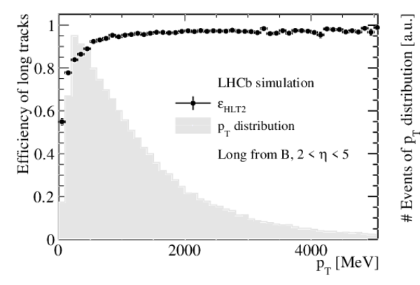
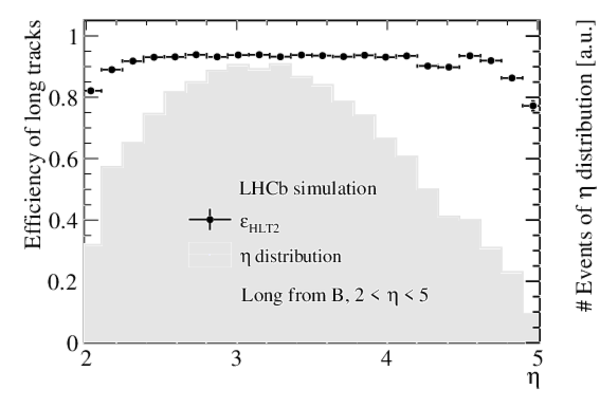
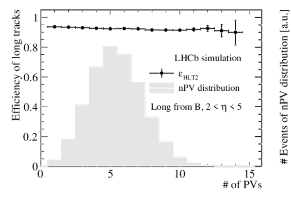
Long track reconstruction efficiency versus momentum $ p$ , transverse momentum $ p_{\mathrm{T}}$ , pseudo-rapidity $\eta$ , and number of primary vertices for long reconstructible particles from $ B $ decays within $2<\eta <5$. Shaded histograms show the distributions of reconstructible particles. |
BestLo[..].pdf [17 KiB] HiDef png [211 KiB] Thumbnail [167 KiB] |
|
|
BestLo[..].pdf [17 KiB] HiDef png [208 KiB] Thumbnail [167 KiB] |
|
|
|
BestLo[..].pdf [15 KiB] HiDef png [190 KiB] Thumbnail [163 KiB] |
|
|
|
BestLo[..].pdf [14 KiB] HiDef png [147 KiB] Thumbnail [83 KiB] |
|
|
|
Ghost rate of long tracks reconstructed by the forward and match tracking algorithms as a function of momentum $ p$ , transverse momentum $ p_{\mathrm{T}}$ , pseudo-rapidity $\eta$ , and number of primary vertices. |
Bestlo[..].pdf [16 KiB] HiDef png [80 KiB] Thumbnail [43 KiB] |

|
|
Bestlo[..].pdf [16 KiB] HiDef png [78 KiB] Thumbnail [42 KiB] |

|
[Failure to get the plot] | [Failure to get the plot] |
|
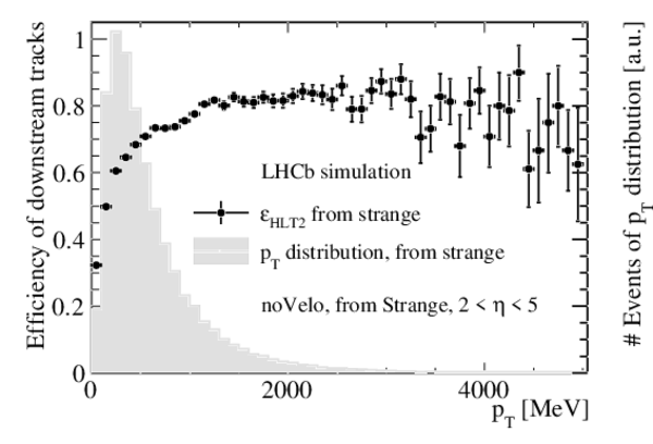
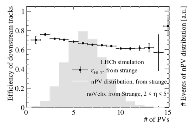
Downstream track reconstruction efficiency versus momentum $ p$ , transverse momentum $ p_{\mathrm{T}}$ , pseudo-rapidity $\eta$ , and number of primary vertices for reconstructible particles from long-lived particle (marked as strange in the legend) decays within $2<\eta <5$ that have no hits in the {\gls*{velo}} . Shaded histograms show the distributions of reconstructible particles. |
BestDo[..].pdf [20 KiB] HiDef png [217 KiB] Thumbnail [121 KiB] |

|
|
BestDo[..].pdf [20 KiB] HiDef png [216 KiB] Thumbnail [121 KiB] |
|
|
|
BestDo[..].pdf [15 KiB] HiDef png [202 KiB] Thumbnail [115 KiB] |

|
|
|
BestDo[..].pdf [15 KiB] HiDef png [189 KiB] Thumbnail [106 KiB] |
|
|
|
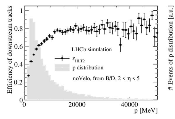
Downstream track reconstruction efficiency versus momentum $ p$ , transverse momentum $ p_{\mathrm{T}}$ , pseudo-rapidity $\eta$ , and number of primary vertices for reconstructible particles from $ B $ / $ D $ decays within $2<\eta <5$ that have no hits in {\gls*{velo}} . Shaded histograms show the distributions of reconstructible particles. |
BestDo[..].pdf [20 KiB] HiDef png [204 KiB] Thumbnail [117 KiB] |
|
|
BestDo[..].pdf [20 KiB] HiDef png [202 KiB] Thumbnail [115 KiB] |

|
|
|
BestDo[..].pdf [16 KiB] HiDef png [176 KiB] Thumbnail [103 KiB] |

|
|
|
BestDo[..].pdf [15 KiB] HiDef png [173 KiB] Thumbnail [98 KiB] |

|
|
|
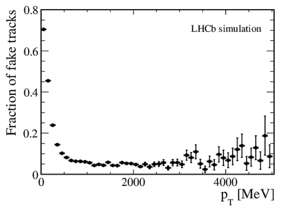
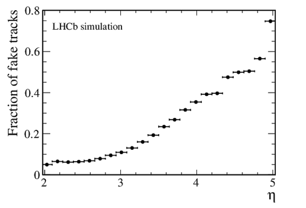
Ghost rate of downstream tracks reconstructed by the forward- and match-tracking algorithms as a function of momentum $ p$ , transverse momentum $ p_{\mathrm{T}}$ , pseudo-rapidity $\eta$ and number of primary vertices. |
BestDo[..].pdf [17 KiB] HiDef png [95 KiB] Thumbnail [55 KiB] |

|
|
BestDo[..].pdf [17 KiB] HiDef png [91 KiB] Thumbnail [49 KiB] |
|
|
|
BestDo[..].pdf [14 KiB] HiDef png [63 KiB] Thumbnail [38 KiB] |
|
|
|
BestDo[..].pdf [14 KiB] HiDef png [69 KiB] Thumbnail [42 KiB] |
|
|
|
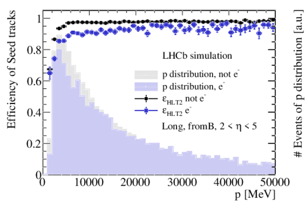
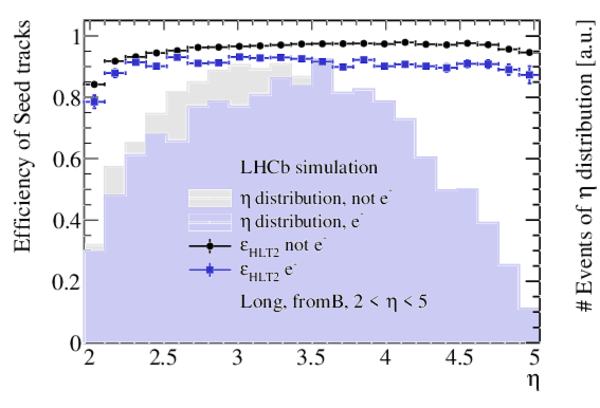
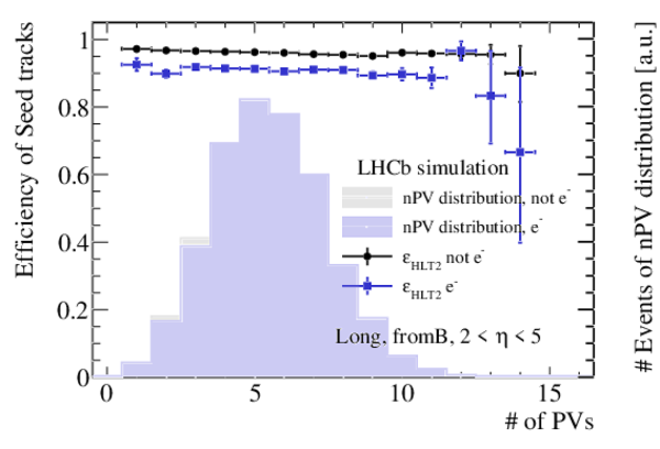
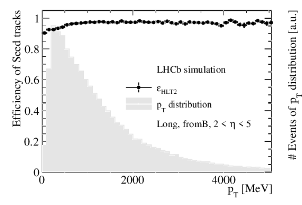
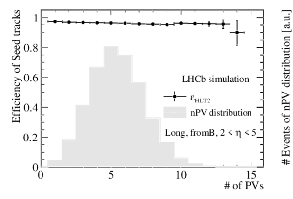
Seeding track-reconstruction efficiency versus momentum $ p$ , transverse momentum $ p_{\mathrm{T}}$ , pseudo-rapidity $\eta$ , and number of primary vertices for long reconstructible electrons (blue squares) and non-electron (black dots) particles within $2<\eta <5$. Shaded histograms show the distributions of reconstructible particles. |
Seed_l[..].pdf [21 KiB] HiDef png [349 KiB] Thumbnail [258 KiB] |
|
|
Seed_l[..].pdf [22 KiB] HiDef png [338 KiB] Thumbnail [250 KiB] |

|
|
|
Seed_l[..].pdf [17 KiB] HiDef png [331 KiB] Thumbnail [237 KiB] |
|
|
|
Seed_l[..].pdf [16 KiB] HiDef png [239 KiB] Thumbnail [191 KiB] |
|
|
|
Seeding track reconstruction efficiency versus momentum $ p$ , transverse momentum $ p_{\mathrm{T}}$ , pseudo-rapidity $\eta$ , and number of primary vertices for long reconstructible particles from $ B $ decays within $2<\eta <5$. Shaded histograms show the distributions of reconstructible particles. |
Seed_l[..].pdf [17 KiB] HiDef png [172 KiB] Thumbnail [94 KiB] |

|
|
Seed_l[..].pdf [17 KiB] HiDef png [172 KiB] Thumbnail [94 KiB] |
|
|
|
Seed_l[..].pdf [15 KiB] HiDef png [155 KiB] Thumbnail [88 KiB] |

|
|
|
Seed_l[..].pdf [14 KiB] HiDef png [148 KiB] Thumbnail [82 KiB] |
|
|
|
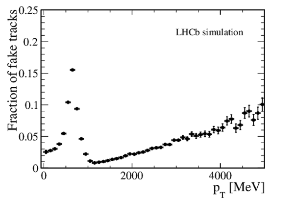
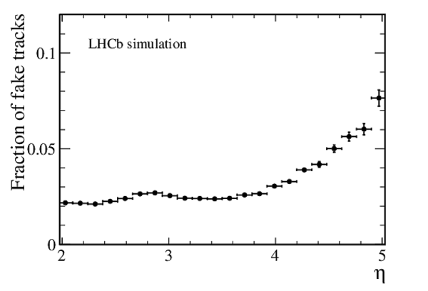
Ghost rate of standalone seeding tracks as a function of momentum $ p$ , transverse momentum $ p_{\mathrm{T}}$ , pseudo-rapidity $\eta$ , and number of primary vertices. The prominent peak in the ghost rate at low transverse momentum (top-right panel) results from a combination of geometric and kinematic effects |
Seed_g[..].pdf [17 KiB] HiDef png [93 KiB] Thumbnail [50 KiB] |

|
|
Seed_g[..].pdf [17 KiB] HiDef png [91 KiB] Thumbnail [51 KiB] |
|
|
|
Seed_g[..].pdf [14 KiB] HiDef png [61 KiB] Thumbnail [35 KiB] |
|
|
|
Seed_g[..].pdf [14 KiB] HiDef png [73 KiB] Thumbnail [43 KiB] |
|
|
|
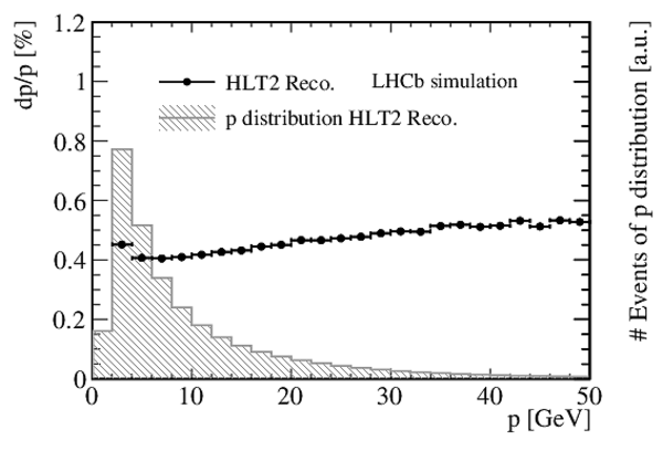
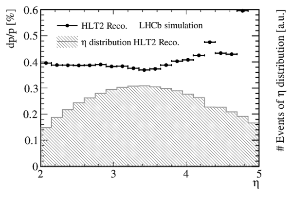
Relative resolution of the momentum of reconstructed tracks as a function of momentum $ p$ , and pseudo-rapidity $\eta $. |
trackr[..].pdf [15 KiB] HiDef png [155 KiB] Thumbnail [92 KiB] |
|
|
trackr[..].pdf [15 KiB] HiDef png [264 KiB] Thumbnail [153 KiB] |
|
|
|
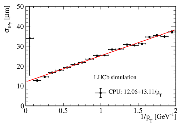
Resolution of the $x$ projection of the impact parameter, $\sigma_{\mathrm{IPx}}$ (left) and $\sigma_{\mathrm{IPy}}$ (right) as a function of the inverse of transverse momentum $1/ p_{\mathrm{T}} $. A minimum bias sample is used for the {\gls*{ip}} resolution study. |
resIPx.pdf [15 KiB] HiDef png [118 KiB] Thumbnail [110 KiB] |

|
|
resIPy.pdf [15 KiB] HiDef png [119 KiB] Thumbnail [111 KiB] |
|
|
|
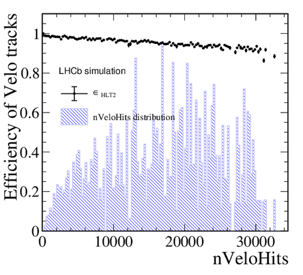
Reconstruction efficiency of (left) {\gls*{velo}} and (right) long tracks as a function of the occupancy in the vertex detector and {\gls*{sft}} , respectively. |
Canvas[..].pdf [19 KiB] HiDef png [580 KiB] Thumbnail [459 KiB] |
|
|
Canvas[..].pdf [24 KiB] HiDef png [508 KiB] Thumbnail [408 KiB] |

|
|
|
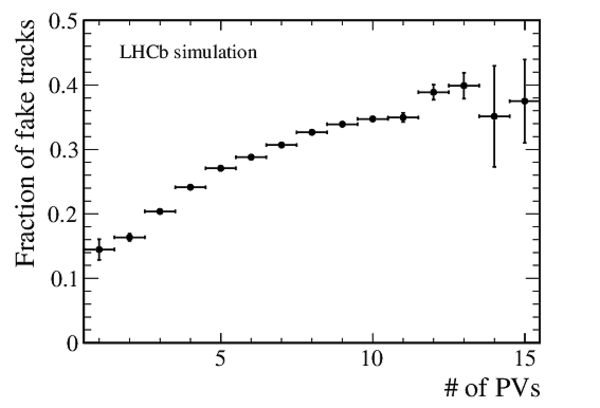
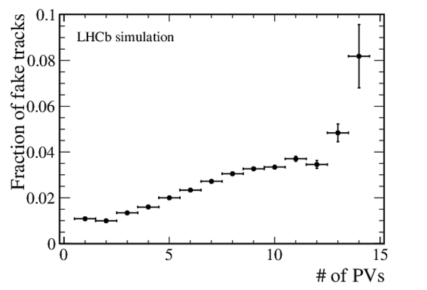
Top: track reconstruction efficiency as a function of the $z$ position of the primary vertex ($PV_z$), for simulated samples with stand-alone (blue) $ p \text{He}$ and (green) {\gls*{prpr}} , and overlapping (red) {\gls*{prpr}} + $ p \text{He}$ and (orange) {\gls*{prpr}} + $ p \text{Ar}$ collisions. The distribution of $PV_z$ for reconstructible {\gls*{pv}} {s} is also shown (shaded histogram, arbitrary units). Bottom: corresponding rate of fake reconstructed tracks as a function of track momentum $ p$ . |
tracki[..].pdf [34 KiB] HiDef png [271 KiB] Thumbnail [186 KiB] |
|
|
tracki[..].pdf [43 KiB] HiDef png [245 KiB] Thumbnail [153 KiB] |
|
|
|
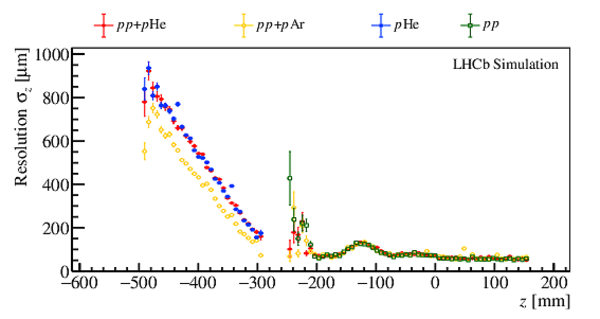
Primary vertex reconstruction (top) efficiency and (bottom) resolution as a function of the $z$ coordinate measured on simulated samples with stand-alone (green) {\gls*{prpr}} , (blue) $ p \text{He}$ and overlapping (red) {\gls*{prpr}} + $ p \text{He}$ and (orange) {\gls*{prpr}} + $ p \text{Ar}$ collisions. |
PV_Eff[..].pdf [47 KiB] HiDef png [252 KiB] Thumbnail [163 KiB] |

|
|
PV_Res[..].pdf [31 KiB] HiDef png [177 KiB] Thumbnail [115 KiB] |
|
|
|
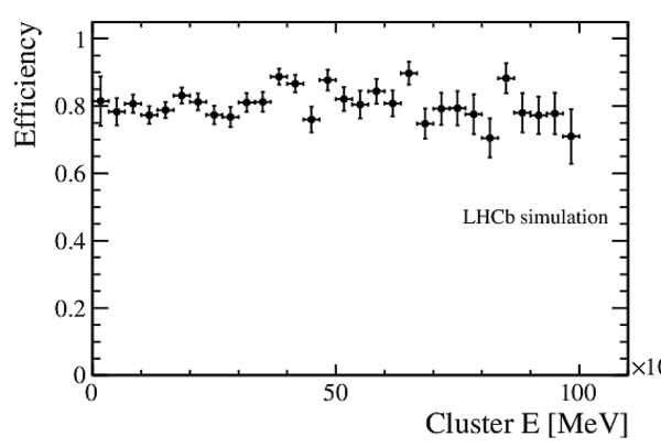
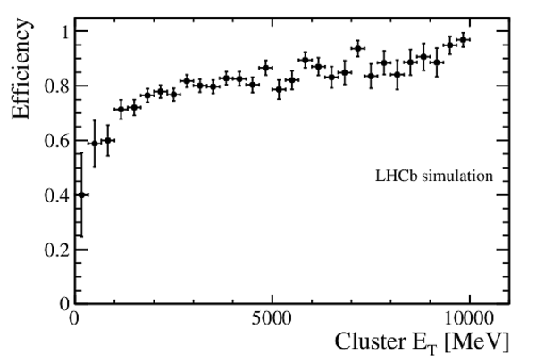
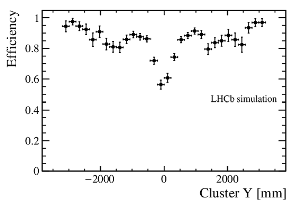
{\gls*{ecal}} cluster reconstruction efficiency versus energy $E$, transverse energy $ E_{\mathrm{T}}$ and $x$ and $y$ position in the {\gls*{ecal}} for reconstructible photons from $ B ^0 \rightarrow K ^{*0} \gamma $ decays. |
eff_cl_e.pdf [16 KiB] HiDef png [83 KiB] Thumbnail [48 KiB] |
|
|
eff_cl_et.pdf [16 KiB] HiDef png [85 KiB] Thumbnail [50 KiB] |
|
|
|
eff_cl_x.pdf [16 KiB] HiDef png [93 KiB] Thumbnail [54 KiB] |

|
|
|
eff_cl_y.pdf [16 KiB] HiDef png [84 KiB] Thumbnail [49 KiB] |
|
|
|
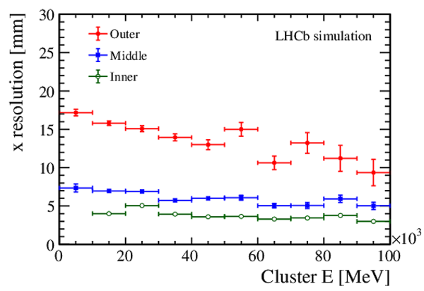
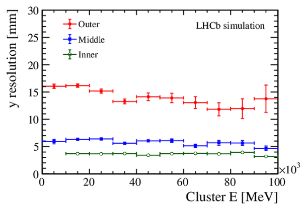
{\gls*{ecal}} -cluster (left) $x$ position and (right) $y$ position resolution versus energy for reconstructible photons from $ B ^0 \rightarrow K ^{*0} \gamma $ decays. |
resolu[..].pdf [15 KiB] HiDef png [151 KiB] Thumbnail [138 KiB] |
|
|
resolu[..].pdf [15 KiB] HiDef png [150 KiB] Thumbnail [137 KiB] |
|
|
|
Merged $\pi ^0$ (left) $x$ position and (right) $y$ position resolution versus energy for ${\pi ^0 \rightarrow \gamma \gamma }$ from $ B $ decays. |
resolu[..].pdf [16 KiB] HiDef png [160 KiB] Thumbnail [147 KiB] |

|
|
resolu[..].pdf [16 KiB] HiDef png [159 KiB] Thumbnail [146 KiB] |

|
|
|
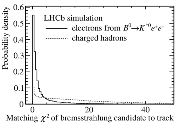
Main electron {\gls*{pid}} variables for the {\gls*{ecal}} : distributions for signal and background separately for the variables (left) EcalE/ $ p$ and (right) matching $\chi^2$ of a bremsstrahlung cluster candidate to a track. The distributions of the bremsstrahlung matching $\chi^2$ are conditional on having a cluster candidate in a $3\times 3$ cell grid around the bremsstrahlung track extrapolation. |
perfor[..].pdf [15 KiB] HiDef png [125 KiB] Thumbnail [73 KiB] |

|
|
perfor[..].pdf [15 KiB] HiDef png [137 KiB] Thumbnail [76 KiB] |
|
|
|
Performance of the {\gls*{hltone}} inclusive selections as a function of (left) parent-particle transverse momentum and (right) parent-particle decay time. The top row plots are the single-track selections, while the bottom row plots are the two-track displaced vertex selections. The signal topologies are indicated in the legend above each plot. The decay time plots are drawn such that the $x$ axis is binned in units of the lifetime for each hadron in its rest frame. |
MultiS[..].pdf [17 KiB] HiDef png [244 KiB] Thumbnail [183 KiB] |

|
|
MultiS[..].pdf [16 KiB] HiDef png [217 KiB] Thumbnail [162 KiB] |

|
|
|
MultiS[..].pdf [17 KiB] HiDef png [253 KiB] Thumbnail [191 KiB] |

|
|
|
MultiS[..].pdf [16 KiB] HiDef png [223 KiB] Thumbnail [170 KiB] |

|
|
|
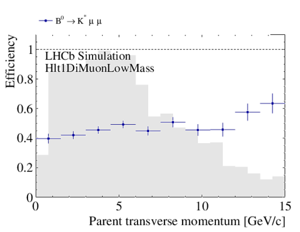
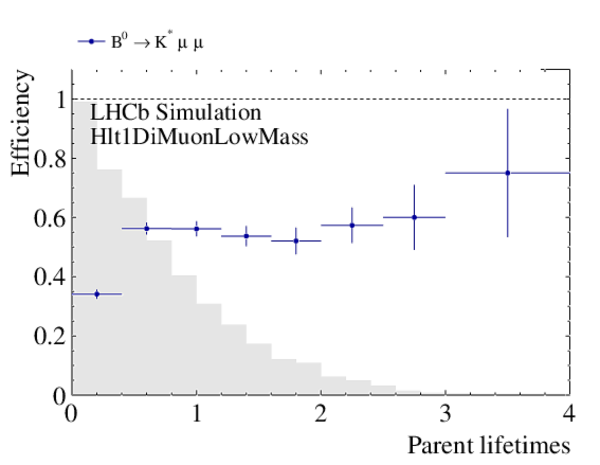
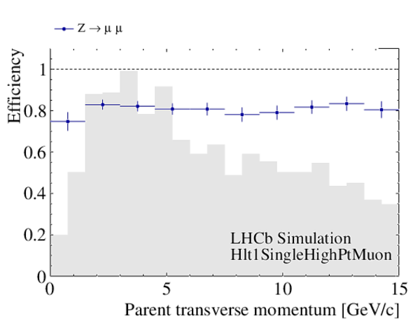
Performance of the {\gls*{hltone}} muon selections. The signal topologies are indicated in the legend above each plot. In the top row the performance of the dimuon selections is plotted as a function of (left) parent-particle transverse momentum and (right) parent-particle decay time. The decay time plot is drawn such that the $x$ axis is binned in units of the lifetime for each hadron in its rest frame. In the bottom row the performance of the single high- $ p_{\mathrm{T}}$ muon selection is plotted as a function of parent transverse momentum. The shaded histograms indicate the distribution of the parent particle prior to any trigger selection. |
MultiS[..].pdf [15 KiB] HiDef png [192 KiB] Thumbnail [151 KiB] |
|
|
MultiS[..].pdf [14 KiB] HiDef png [161 KiB] Thumbnail [128 KiB] |
|
|
|
MultiS[..].pdf [15 KiB] HiDef png [199 KiB] Thumbnail [158 KiB] |
|
|
|
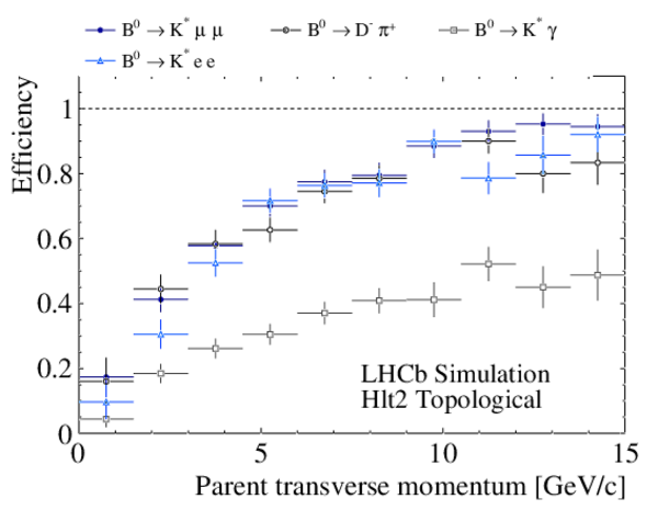
Performance of the {\gls*{hlttwo}} inclusive selections. The signal topologies are indicated in the legend above each plot. In the top row the performance of the inclusive displaced-vertex selections is plotted as a function of (left) parent-particle transverse momentum and (right) parent-particle decay time. The decay-time plot is drawn such that the $x$ axis is binned in units of the lifetime for each hadron in its rest frame. In the bottom row the performance of the single high- $ p_{\mathrm{T}}$ muon selection is plotted as a function of parent transverse momentum. The shaded histograms indicate the distribution of the parent particle prior to any trigger selection. |
MultiS[..].pdf [16 KiB] HiDef png [231 KiB] Thumbnail [173 KiB] |
|
|
MultiS[..].pdf [16 KiB] HiDef png [201 KiB] Thumbnail [152 KiB] |

|
|
|
MultiS[..].pdf [14 KiB] HiDef png [195 KiB] Thumbnail [152 KiB] |

|
|
|
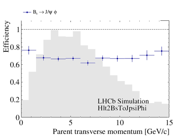
Performance of example {\gls*{hlttwo}} exclusive selections as a function of (left) parent-particle transverse momentum and (right) parent-particle decay time. The signal topologies are indicated in the legend above each plot. The decay-time plots are drawn such that the $x$ axis is binned in units of the lifetime for each hadron in its rest frame. The shaded histograms indicate the distribution of the parent particle prior to any trigger selection. |
MultiS[..].pdf [15 KiB] HiDef png [193 KiB] Thumbnail [152 KiB] |
|
|
MultiS[..].pdf [14 KiB] HiDef png [158 KiB] Thumbnail [125 KiB] |

|
|
|
MultiS[..].pdf [14 KiB] HiDef png [196 KiB] Thumbnail [151 KiB] |

|
|
|
MultiS[..].pdf [14 KiB] HiDef png [171 KiB] Thumbnail [137 KiB] |

|
|
|
Animated gif made out of all figures. |
DP-2022-002.gif Thumbnail |

|
![HiDef png [159 KiB]](Directory_LHCb-DP-2022-002/hidef_plot-hans.png)
![HiDef png [189 KiB]](Directory_LHCb-DP-2022-002/hidef_ratesptGP.png)
![LHCb-u[..].jpg [195 KiB]](Directory_LHCb-DP-2022-002/LHCb-upgrade-y.jpg)
![HiDef png [539 KiB]](Directory_LHCb-DP-2022-002/hidef_LHCb-upgrade-y.png)
![electr[..].jpg [313 KiB]](Directory_LHCb-DP-2022-002/electronics_archi.jpg)
![HiDef png [370 KiB]](Directory_LHCb-DP-2022-002/hidef_electronics_archi.png)
![Cavern[..].jpg [307 KiB]](Directory_LHCb-DP-2022-002/CavernAndDataCentre.jpg)
![HiDef png [784 KiB]](Directory_LHCb-DP-2022-002/hidef_CavernAndDataCentre.png)
![plume-bm.jpg [475 KiB]](Directory_LHCb-DP-2022-002/plume-bm.jpg)
![HiDef png [2 MiB]](Directory_LHCb-DP-2022-002/hidef_plume-bm.png)
![BCM.jpg [369 KiB]](Directory_LHCb-DP-2022-002/BCM.jpg)
![HiDef png [2 MiB]](Directory_LHCb-DP-2022-002/hidef_BCM.png)
![elem_det_a.jpg [176 KiB]](Directory_LHCb-DP-2022-002/elem_det_a.jpg)
![HiDef png [263 KiB]](Directory_LHCb-DP-2022-002/hidef_elem_det_a.png)
![IMG-TB-new.jpg [402 KiB]](Directory_LHCb-DP-2022-002/IMG-TB-new.jpg)
![HiDef png [1 MiB]](Directory_LHCb-DP-2022-002/hidef_IMG-TB-new.png)
![RunID_[..].jpg [145 KiB]](Directory_LHCb-DP-2022-002/RunID_023_hodoscop01_L01-new.jpg)
![HiDef png [291 KiB]](Directory_LHCb-DP-2022-002/hidef_RunID_023_hodoscop01_L01-new.png)
![HiDef png [1 MiB]](Directory_LHCb-DP-2022-002/hidef_dataRatePerAsic.png)
![zlayou[..].jpg [96 KiB]](Directory_LHCb-DP-2022-002/zlayout_from_PUB-2019-008.jpg)
![HiDef png [149 KiB]](Directory_LHCb-DP-2022-002/hidef_zlayout_from_PUB-2019-008.png)
![Schema[..].jpg [129 KiB]](Directory_LHCb-DP-2022-002/SchematicWithPixelsAndPhoto.jpg)
![HiDef png [1 MiB]](Directory_LHCb-DP-2022-002/hidef_SchematicWithPixelsAndPhoto.png)
![Thumbnail [221 KiB]](Directory_LHCb-DP-2022-002/thumbnail_SchematicWithPixelsAndPhoto.png)
![HiDef png [1 MiB]](Directory_LHCb-DP-2022-002/hidef_Cooling_substrate_cropped.png)
![HiDef png [2 MiB]](Directory_LHCb-DP-2022-002/hidef_microchannelXray.png)
![Coolin[..].jpg [205 KiB]](Directory_LHCb-DP-2022-002/Cooling_alignement.jpg)
![HiDef png [1 MiB]](Directory_LHCb-DP-2022-002/hidef_Cooling_alignement.png)
![Coolin[..].jpg [219 KiB]](Directory_LHCb-DP-2022-002/Cooling_xray.jpg)
![HiDef png [196 KiB]](Directory_LHCb-DP-2022-002/hidef_Cooling_xray.png)
![module[..].jpg [178 KiB]](Directory_LHCb-DP-2022-002/module_annotated_cropped.jpg)
![HiDef png [1 MiB]](Directory_LHCb-DP-2022-002/hidef_module_annotated_cropped.png)
![BareMo[..].jpg [756 KiB]](Directory_LHCb-DP-2022-002/BareModule_Cside.jpg)
![HiDef png [4 MiB]](Directory_LHCb-DP-2022-002/hidef_BareModule_Cside.png)
![TilesM[..].jpg [735 KiB]](Directory_LHCb-DP-2022-002/TilesModule_Cside.jpg)
![HiDef png [4 MiB]](Directory_LHCb-DP-2022-002/hidef_TilesModule_Cside.png)
![Hybrid[..].jpg [724 KiB]](Directory_LHCb-DP-2022-002/HybridsModule_Cside.jpg)
![HiDef png [4 MiB]](Directory_LHCb-DP-2022-002/hidef_HybridsModule_Cside.png)
![202112[..].jpg [508 KiB]](Directory_LHCb-DP-2022-002/20211209_substratemarker7.jpg)
![HiDef png [2 MiB]](Directory_LHCb-DP-2022-002/hidef_20211209_substratemarker7.png)
![202112[..].jpg [611 KiB]](Directory_LHCb-DP-2022-002/20211209_CLImarker2.jpg)
![HiDef png [2 MiB]](Directory_LHCb-DP-2022-002/hidef_20211209_CLImarker2.png)
![202112[..].jpg [1 MiB]](Directory_LHCb-DP-2022-002/20211209_sensormarkersCLI_1256.jpg)
![HiDef png [2 MiB]](Directory_LHCb-DP-2022-002/hidef_20211209_sensormarkersCLI_1256.png)
![TileMe[..].jpg [102 KiB]](Directory_LHCb-DP-2022-002/TileMetrology_corrected.jpg)
![HiDef png [220 KiB]](Directory_LHCb-DP-2022-002/hidef_TileMetrology_corrected.png)
![HiDef png [213 KiB]](Directory_LHCb-DP-2022-002/hidef_VELOElectronicsDiagram.png)
![hybrid[..].jpg [118 KiB]](Directory_LHCb-DP-2022-002/hybrids_annotated.jpg)
![HiDef png [809 KiB]](Directory_LHCb-DP-2022-002/hidef_hybrids_annotated.png)
![Vacuum[..].jpg [144 KiB]](Directory_LHCb-DP-2022-002/VacuumFeedthrough_annotated.jpg)
![HiDef png [882 KiB]](Directory_LHCb-DP-2022-002/hidef_VacuumFeedthrough_annotated.png)
![halfas[..].jpg [123 KiB]](Directory_LHCb-DP-2022-002/halfassembly_new.jpg)
![HiDef png [2 MiB]](Directory_LHCb-DP-2022-002/hidef_halfassembly_new.png)
![CAD_wh[..].jpg [366 KiB]](Directory_LHCb-DP-2022-002/CAD_whole_internal.jpg)
![HiDef png [810 KiB]](Directory_LHCb-DP-2022-002/hidef_CAD_whole_internal.png)
![RFboxI[..].jpg [111 KiB]](Directory_LHCb-DP-2022-002/RFboxInstallation.jpg)
![HiDef png [783 KiB]](Directory_LHCb-DP-2022-002/hidef_RFboxInstallation.png)
![PrincS[..].png [69 KiB]](Directory_LHCb-DP-2022-002/PrincStorageTube-new.png)
![HiDef png [57 KiB]](Directory_LHCb-DP-2022-002/hidef_PrincStorageTube-new.png)
![overal[..].png [230 KiB]](Directory_LHCb-DP-2022-002/overall_2_cropped.png)
![HiDef png [890 KiB]](Directory_LHCb-DP-2022-002/hidef_overall_2_cropped.png)
![cell_o[..].png [214 KiB]](Directory_LHCb-DP-2022-002/cell_opened_cropped.png)
![HiDef png [596 KiB]](Directory_LHCb-DP-2022-002/hidef_cell_opened_cropped.png)
![photo-[..].jpg [956 KiB]](Directory_LHCb-DP-2022-002/photo-cell-vessel.jpg)
![HiDef png [2 MiB]](Directory_LHCb-DP-2022-002/hidef_photo-cell-vessel.png)
![2018_1[..].png [271 KiB]](Directory_LHCb-DP-2022-002/2018_10_17_table_GFS_BP_SV_RGA_GG_NG_V1.png)
![HiDef png [309 KiB]](Directory_LHCb-DP-2022-002/hidef_2018_10_17_table_GFS_BP_SV_RGA_GG_NG_V1.png)
![UT_planes.jpg [131 KiB]](Directory_LHCb-DP-2022-002/UT_planes.jpg)
![HiDef png [997 KiB]](Directory_LHCb-DP-2022-002/hidef_UT_planes.png)
![HiDef png [2 MiB]](Directory_LHCb-DP-2022-002/hidef_ut_generalview.png)
![HiDef png [2 MiB]](Directory_LHCb-DP-2022-002/hidef_stave-figure.png)
![typed_[..].jpg [75 KiB]](Directory_LHCb-DP-2022-002/typed_cutout.jpg)
![HiDef png [1 MiB]](Directory_LHCb-DP-2022-002/hidef_typed_cutout.png)
![pa_photo.jpg [287 KiB]](Directory_LHCb-DP-2022-002/pa_photo.jpg)
![HiDef png [2 MiB]](Directory_LHCb-DP-2022-002/hidef_pa_photo.png)
![HiDef png [110 KiB]](Directory_LHCb-DP-2022-002/hidef_salt_block.png)
![veraHybrid.jpg [521 KiB]](Directory_LHCb-DP-2022-002/veraHybrid.jpg)
![HiDef png [2 MiB]](Directory_LHCb-DP-2022-002/hidef_veraHybrid.png)
![module[..].jpg [198 KiB]](Directory_LHCb-DP-2022-002/module-D-new.jpg)
![HiDef png [1 MiB]](Directory_LHCb-DP-2022-002/hidef_module-D-new.png)
![Flex1.jpg [141 KiB]](Directory_LHCb-DP-2022-002/Flex1.jpg)
![HiDef png [623 KiB]](Directory_LHCb-DP-2022-002/hidef_Flex1.png)
![pigtails.jpg [1 MiB]](Directory_LHCb-DP-2022-002/pigtails.jpg)
![HiDef png [2 MiB]](Directory_LHCb-DP-2022-002/hidef_pigtails.png)
![ptribbons.jpg [76 KiB]](Directory_LHCb-DP-2022-002/ptribbons.jpg)
![HiDef png [1 MiB]](Directory_LHCb-DP-2022-002/hidef_ptribbons.png)
![instal[..].jpg [156 KiB]](Directory_LHCb-DP-2022-002/installationpigtails.jpg)
![HiDef png [1 MiB]](Directory_LHCb-DP-2022-002/hidef_installationpigtails.png)
![Data_C[..].jpg [610 KiB]](Directory_LHCb-DP-2022-002/Data_Control_Flow.jpg)
![HiDef png [683 KiB]](Directory_LHCb-DP-2022-002/hidef_Data_Control_Flow.png)
![Flex2.jpg [267 KiB]](Directory_LHCb-DP-2022-002/Flex2.jpg)
![HiDef png [1 MiB]](Directory_LHCb-DP-2022-002/hidef_Flex2.png)
![hybrid[..].jpg [54 KiB]](Directory_LHCb-DP-2022-002/hybrid_power_groups.jpg)
![HiDef png [544 KiB]](Directory_LHCb-DP-2022-002/hidef_hybrid_power_groups.png)
![utcooling1.jpg [398 KiB]](Directory_LHCb-DP-2022-002/utcooling1.jpg)
![HiDef png [277 KiB]](Directory_LHCb-DP-2022-002/hidef_utcooling1.png)
![HiDef png [377 KiB]](Directory_LHCb-DP-2022-002/hidef_FermilabTBResults.png)
![HiDef png [395 KiB]](Directory_LHCb-DP-2022-002/hidef_ut_slice_test_noise_comparison.png)
![HiDef png [84 KiB]](Directory_LHCb-DP-2022-002/hidef_matthickness_vs_eta.png)
![ut_occ[..].jpg [123 KiB]](Directory_LHCb-DP-2022-002/ut_occupancy.jpg)
![HiDef png [387 KiB]](Directory_LHCb-DP-2022-002/hidef_ut_occupancy.png)
![HiDef png [1 MiB]](Directory_LHCb-DP-2022-002/hidef_3stations_3m_A3_3.png)
![dosemap_T1.jpg [173 KiB]](Directory_LHCb-DP-2022-002/dosemap_T1.jpg)
![HiDef png [204 KiB]](Directory_LHCb-DP-2022-002/hidef_dosemap_T1.png)
![fibree[..].jpg [279 KiB]](Directory_LHCb-DP-2022-002/fibreend-new.jpg)
![HiDef png [1 MiB]](Directory_LHCb-DP-2022-002/hidef_fibreend-new.png)
![fibremat.jpg [160 KiB]](Directory_LHCb-DP-2022-002/fibremat.jpg)
![HiDef png [1 MiB]](Directory_LHCb-DP-2022-002/hidef_fibremat.png)
![SCIFI-[..].jpg [142 KiB]](Directory_LHCb-DP-2022-002/SCIFI-MODULE-2.jpg)
![HiDef png [441 KiB]](Directory_LHCb-DP-2022-002/hidef_SCIFI-MODULE-2.png)
![HiDef png [63 KiB]](Directory_LHCb-DP-2022-002/hidef_radlengthsim.png)
![HiDef png [3 MiB]](Directory_LHCb-DP-2022-002/hidef_h2017_array.png)
![HiDef png [375 KiB]](Directory_LHCb-DP-2022-002/hidef_dcr_6e11.png)
![HiDef png [5 MiB]](Directory_LHCb-DP-2022-002/hidef_HALFROB.png)
![HiDef png [833 KiB]](Directory_LHCb-DP-2022-002/hidef_BlockSchematicData.png)
![HiDef png [57 KiB]](Directory_LHCb-DP-2022-002/hidef_pacific_block.png)
![HiDef png [168 KiB]](Directory_LHCb-DP-2022-002/hidef_shaper_20220104.png)
![HiDef png [206 KiB]](Directory_LHCb-DP-2022-002/hidef_p5q_pz6_20220104.png)
![HiDef png [152 KiB]](Directory_LHCb-DP-2022-002/hidef_ScurveFit.png)
![HiDef png [149 KiB]](Directory_LHCb-DP-2022-002/hidef_clusteringdiagram.png)
![HiDef png [2 MiB]](Directory_LHCb-DP-2022-002/hidef_coldbox.png)
![HiDef png [1 MiB]](Directory_LHCb-DP-2022-002/hidef_attenmap.png)
![HiDef png [145 KiB]](Directory_LHCb-DP-2022-002/hidef_toy_fit_comp_T15_25_45_v3.png)
![HiDef png [56 KiB]](Directory_LHCb-DP-2022-002/hidef_hondie_5ns.png)
![HiDef png [454 KiB]](Directory_LHCb-DP-2022-002/hidef_doublegausfit.png)
![rich1l[..].jpg [341 KiB]](Directory_LHCb-DP-2022-002/rich1layout.jpg)
![HiDef png [3 MiB]](Directory_LHCb-DP-2022-002/hidef_rich1layout.png)
![rich2l[..].jpg [881 KiB]](Directory_LHCb-DP-2022-002/rich2layoutMirrored.jpg)
![HiDef png [1 MiB]](Directory_LHCb-DP-2022-002/hidef_rich2layoutMirrored.png)
![HiDef png [3 MiB]](Directory_LHCb-DP-2022-002/hidef_MaPMTs.png)
![multia[..].jpg [235 KiB]](Directory_LHCb-DP-2022-002/multianodev4.jpg)
![HiDef png [368 KiB]](Directory_LHCb-DP-2022-002/hidef_multianodev4.png)
![MaPMTs[..].jpg [345 KiB]](Directory_LHCb-DP-2022-002/MaPMTspectra.jpg)
![HiDef png [399 KiB]](Directory_LHCb-DP-2022-002/hidef_MaPMTspectra.png)
![MaPMT_[..].jpg [85 KiB]](Directory_LHCb-DP-2022-002/MaPMT_QE_axis.jpg)
![HiDef png [464 KiB]](Directory_LHCb-DP-2022-002/hidef_MaPMT_QE_axis.png)
![claroChip.jpg [329 KiB]](Directory_LHCb-DP-2022-002/claroChip.jpg)
![HiDef png [2 MiB]](Directory_LHCb-DP-2022-002/hidef_claroChip.png)
![claroS[..].jpg [104 KiB]](Directory_LHCb-DP-2022-002/claroScheme.jpg)
![HiDef png [148 KiB]](Directory_LHCb-DP-2022-002/hidef_claroScheme.png)
![ECRexp[..].jpg [497 KiB]](Directory_LHCb-DP-2022-002/ECRexploded.jpg)
![HiDef png [347 KiB]](Directory_LHCb-DP-2022-002/hidef_ECRexploded.png)
![withoutMS.jpg [90 KiB]](Directory_LHCb-DP-2022-002/withoutMS.jpg)
![HiDef png [177 KiB]](Directory_LHCb-DP-2022-002/hidef_withoutMS.png)
![withMS.jpg [81 KiB]](Directory_LHCb-DP-2022-002/withMS.jpg)
![HiDef png [160 KiB]](Directory_LHCb-DP-2022-002/hidef_withMS.png)
![ECHexp[..].jpg [241 KiB]](Directory_LHCb-DP-2022-002/ECHexploded.jpg)
![HiDef png [267 KiB]](Directory_LHCb-DP-2022-002/hidef_ECHexploded.png)
![pdmdbr.jpg [499 KiB]](Directory_LHCb-DP-2022-002/pdmdbr.jpg)
![HiDef png [2 MiB]](Directory_LHCb-DP-2022-002/hidef_pdmdbr.png)
![pdmdbr[..].jpg [115 KiB]](Directory_LHCb-DP-2022-002/pdmdbrSchematic.jpg)
![HiDef png [719 KiB]](Directory_LHCb-DP-2022-002/hidef_pdmdbrSchematic.png)
![R1col.jpg [186 KiB]](Directory_LHCb-DP-2022-002/R1col.jpg)
![HiDef png [4 MiB]](Directory_LHCb-DP-2022-002/hidef_R1col.png)
![202007[..].jpg [811 KiB]](Directory_LHCb-DP-2022-002/20200727_134921-2.jpg)
![HiDef png [4 MiB]](Directory_LHCb-DP-2022-002/hidef_20200727_134921-2.png)
![RICH1-[..].jpg [95 KiB]](Directory_LHCb-DP-2022-002/RICH1-optics-orig.jpg)
![HiDef png [367 KiB]](Directory_LHCb-DP-2022-002/hidef_RICH1-optics-orig.png)
![RICH1-[..].jpg [99 KiB]](Directory_LHCb-DP-2022-002/RICH1-optics-upgr.jpg)
![HiDef png [371 KiB]](Directory_LHCb-DP-2022-002/hidef_RICH1-optics-upgr.png)
![gas-en[..].jpg [155 KiB]](Directory_LHCb-DP-2022-002/gas-enclosure-CAD.jpg)
![HiDef png [2 MiB]](Directory_LHCb-DP-2022-002/hidef_gas-enclosure-CAD.png)
![gasEnc[..].jpg [543 KiB]](Directory_LHCb-DP-2022-002/gasEnclosureCavern.jpg)
![HiDef png [3 MiB]](Directory_LHCb-DP-2022-002/hidef_gasEnclosureCavern.png)
![rich1s[..].jpg [51 KiB]](Directory_LHCb-DP-2022-002/rich1spherical.jpg)
![HiDef png [1 MiB]](Directory_LHCb-DP-2022-002/hidef_rich1spherical.png)
![rich1flat.jpg [169 KiB]](Directory_LHCb-DP-2022-002/rich1flat.jpg)
![HiDef png [2 MiB]](Directory_LHCb-DP-2022-002/hidef_rich1flat.png)
![rich1box.jpg [301 KiB]](Directory_LHCb-DP-2022-002/rich1box.jpg)
![HiDef png [2 MiB]](Directory_LHCb-DP-2022-002/hidef_rich1box.png)
![RICH2-[..].jpg [404 KiB]](Directory_LHCb-DP-2022-002/RICH2-Photondetector-Assembly-CF210525-1548.jpg)
![HiDef png [2 MiB]](Directory_LHCb-DP-2022-002/hidef_RICH2-Photondetector-Assembly-CF210525-1548.png)
![rich2_[..].jpg [159 KiB]](Directory_LHCb-DP-2022-002/rich2_Aside.jpg)
![HiDef png [3 MiB]](Directory_LHCb-DP-2022-002/hidef_rich2_Aside.png)
![RICH2-[..].jpg [417 KiB]](Directory_LHCb-DP-2022-002/RICH2-Photodetector-Enclosure-CF210525-1622.jpg)
![HiDef png [1 MiB]](Directory_LHCb-DP-2022-002/hidef_RICH2-Photodetector-Enclosure-CF210525-1622.png)
![RICH2-[..].jpg [1 MiB]](Directory_LHCb-DP-2022-002/RICH2-Photodetector-Enclosure-20210415_181949-2.jpg)
![HiDef png [5 MiB]](Directory_LHCb-DP-2022-002/hidef_RICH2-Photodetector-Enclosure-20210415_181949-2.png)
![single[..].jpg [222 KiB]](Directory_LHCb-DP-2022-002/singleChannelDAC-new.jpg)
![HiDef png [172 KiB]](Directory_LHCb-DP-2022-002/hidef_singleChannelDAC-new.png)
![thresh[..].jpg [199 KiB]](Directory_LHCb-DP-2022-002/thresholdStep-new.jpg)
![HiDef png [340 KiB]](Directory_LHCb-DP-2022-002/hidef_thresholdStep-new.png)
![HiDef png [145 KiB]](Directory_LHCb-DP-2022-002/hidef_rich2workingPointsAndGains.png)
![HiDef png [134 KiB]](Directory_LHCb-DP-2022-002/hidef_qeAverage.png)
![occupa[..].jpg [128 KiB]](Directory_LHCb-DP-2022-002/occupancy-rich1.jpg)
![HiDef png [200 KiB]](Directory_LHCb-DP-2022-002/hidef_occupancy-rich1.png)
![occupa[..].jpg [161 KiB]](Directory_LHCb-DP-2022-002/occupancy-rich2.jpg)
![HiDef png [243 KiB]](Directory_LHCb-DP-2022-002/hidef_occupancy-rich2.png)
![Calo_s[..].png [178 KiB]](Directory_LHCb-DP-2022-002/Calo_segmentation.png)
![HiDef png [108 KiB]](Directory_LHCb-DP-2022-002/hidef_Calo_segmentation.png)
![Calo_E[..].jpg [271 KiB]](Directory_LHCb-DP-2022-002/Calo_ECAL_cell.jpg)
![HiDef png [498 KiB]](Directory_LHCb-DP-2022-002/hidef_Calo_ECAL_cell.png)
![Calo_H[..].jpg [237 KiB]](Directory_LHCb-DP-2022-002/Calo_HCAL_cell.jpg)
![HiDef png [518 KiB]](Directory_LHCb-DP-2022-002/hidef_Calo_HCAL_cell.png)
![Calo_F[..].jpg [245 KiB]](Directory_LHCb-DP-2022-002/Calo_FEB_picture.jpg)
![HiDef png [2 MiB]](Directory_LHCb-DP-2022-002/hidef_Calo_FEB_picture.png)
![HiDef png [301 KiB]](Directory_LHCb-DP-2022-002/hidef_ICECALv3_blocks.png)
![Calo_crate.png [194 KiB]](Directory_LHCb-DP-2022-002/Calo_crate.png)
![HiDef png [184 KiB]](Directory_LHCb-DP-2022-002/hidef_Calo_crate.png)
![DCS_GBT.jpg [262 KiB]](Directory_LHCb-DP-2022-002/DCS_GBT.jpg)
![HiDef png [82 KiB]](Directory_LHCb-DP-2022-002/hidef_DCS_GBT.png)
![HiDef png [502 KiB]](Directory_LHCb-DP-2022-002/hidef_Calo_TB_spillOver.png)
![HiDef png [194 KiB]](Directory_LHCb-DP-2022-002/hidef_Calo_TB_linearity.png)
![HiDef png [165 KiB]](Directory_LHCb-DP-2022-002/hidef_Calo_TB_NL.png)
![HiDef png [530 KiB]](Directory_LHCb-DP-2022-002/hidef_Calo_noise.png)
![nOde_s[..].png [85 KiB]](Directory_LHCb-DP-2022-002/nOde_scheme.png)
![HiDef png [70 KiB]](Directory_LHCb-DP-2022-002/hidef_nOde_scheme.png)
![nOde_s[..].png [275 KiB]](Directory_LHCb-DP-2022-002/nOde_schemeGen.png)
![HiDef png [192 KiB]](Directory_LHCb-DP-2022-002/hidef_nOde_schemeGen.png)
![nSB_scheme.png [201 KiB]](Directory_LHCb-DP-2022-002/nSB_scheme.png)
![HiDef png [143 KiB]](Directory_LHCb-DP-2022-002/hidef_nSB_scheme.png)
![nSB_sc[..].png [271 KiB]](Directory_LHCb-DP-2022-002/nSB_schemeGen.png)
![HiDef png [227 KiB]](Directory_LHCb-DP-2022-002/hidef_nSB_schemeGen.png)
![HiDef png [946 KiB]](Directory_LHCb-DP-2022-002/hidef_nODE_BD.png)
![nODE_L[..].png [167 KiB]](Directory_LHCb-DP-2022-002/nODE_Layout.png)
![HiDef png [721 KiB]](Directory_LHCb-DP-2022-002/hidef_nODE_Layout.png)
![nSYNCd[..].png [244 KiB]](Directory_LHCb-DP-2022-002/nSYNCdiagram.png)
![HiDef png [494 KiB]](Directory_LHCb-DP-2022-002/hidef_nSYNCdiagram.png)
![nSBS_BD.png [60 KiB]](Directory_LHCb-DP-2022-002/nSBS_BD.png)
![HiDef png [109 KiB]](Directory_LHCb-DP-2022-002/hidef_nSBS_BD.png)
![nSBS_ECS.png [43 KiB]](Directory_LHCb-DP-2022-002/nSBS_ECS.png)
![HiDef png [318 KiB]](Directory_LHCb-DP-2022-002/hidef_nSBS_ECS.png)
![nSBS_TFC.png [41 KiB]](Directory_LHCb-DP-2022-002/nSBS_TFC.png)
![HiDef png [306 KiB]](Directory_LHCb-DP-2022-002/hidef_nSBS_TFC.png)
![nFSM.jpg [237 KiB]](Directory_LHCb-DP-2022-002/nFSM.jpg)
![HiDef png [275 KiB]](Directory_LHCb-DP-2022-002/hidef_nFSM.png)
![tungst[..].jpg [274 KiB]](Directory_LHCb-DP-2022-002/tungsten_plug.jpg)
![HiDef png [1018 KiB]](Directory_LHCb-DP-2022-002/hidef_tungsten_plug.png)
![M2R2.jpg [1013 KiB]](Directory_LHCb-DP-2022-002/M2R2.jpg)
![HiDef png [1 MiB]](Directory_LHCb-DP-2022-002/hidef_M2R2.png)
![M2R1.jpg [1006 KiB]](Directory_LHCb-DP-2022-002/M2R1.jpg)
![HiDef png [1 MiB]](Directory_LHCb-DP-2022-002/hidef_M2R1.png)
![MWPC_L[..].jpg [372 KiB]](Directory_LHCb-DP-2022-002/MWPC_LongOp_fig4.jpg)
![HiDef png [586 KiB]](Directory_LHCb-DP-2022-002/hidef_MWPC_LongOp_fig4.png)
![MWPC_L[..].png [78 KiB]](Directory_LHCb-DP-2022-002/MWPC_LongOp_fig8.png)
![HiDef png [192 KiB]](Directory_LHCb-DP-2022-002/hidef_MWPC_LongOp_fig8.png)
![lhcb-o[..].png [272 KiB]](Directory_LHCb-DP-2022-002/lhcb-online-system-2021.png)
![HiDef png [305 KiB]](Directory_LHCb-DP-2022-002/hidef_lhcb-online-system-2021.png)
![PCIe40[..].png [422 KiB]](Directory_LHCb-DP-2022-002/PCIe40_Final_1.png)
![HiDef png [1009 KiB]](Directory_LHCb-DP-2022-002/hidef_PCIe40_Final_1.png)
![TELL40[..].png [156 KiB]](Directory_LHCb-DP-2022-002/TELL40_firmware_architecture.png)
![HiDef png [210 KiB]](Directory_LHCb-DP-2022-002/hidef_TELL40_firmware_architecture.png)
![TFClog[..].PNG [77 KiB]](Directory_LHCb-DP-2022-002/TFClogicalview.PNG)
![HiDef png [231 KiB]](Directory_LHCb-DP-2022-002/hidef_TFClogicalview.png)
![ecs-global.png [149 KiB]](Directory_LHCb-DP-2022-002/ecs-global.png)
![HiDef png [175 KiB]](Directory_LHCb-DP-2022-002/hidef_ecs-global.png)
![HiDef png [351 KiB]](Directory_LHCb-DP-2022-002/hidef_ecs-arch.png)
![fe-ecs.png [12 KiB]](Directory_LHCb-DP-2022-002/fe-ecs.png)
![HiDef png [42 KiB]](Directory_LHCb-DP-2022-002/hidef_fe-ecs.png)
![RunCon[..].jpg [736 KiB]](Directory_LHCb-DP-2022-002/RunControl_Nov22.jpg)
![HiDef png [874 KiB]](Directory_LHCb-DP-2022-002/hidef_RunControl_Nov22.png)
![eb_sca[..].png [45 KiB]](Directory_LHCb-DP-2022-002/eb_scalability_tot_bw_jun2021.png)
![HiDef png [169 KiB]](Directory_LHCb-DP-2022-002/hidef_eb_scalability_tot_bw_jun2021.png)
![HiDef png [293 KiB]](Directory_LHCb-DP-2022-002/hidef_RTA_dataflow_widescreen_norefs.png)
![HiDef png [46 KiB]](Directory_LHCb-DP-2022-002/hidef_Fig_109.png)
![track_[..].png [243 KiB]](Directory_LHCb-DP-2022-002/track_types.png)
![HiDef png [165 KiB]](Directory_LHCb-DP-2022-002/hidef_track_types.png)
![CALO_S[..].png [305 KiB]](Directory_LHCb-DP-2022-002/CALO_Shower_Shapes.png)
![HiDef png [197 KiB]](Directory_LHCb-DP-2022-002/hidef_CALO_Shower_Shapes.png)
![HiDef png [277 KiB]](Directory_LHCb-DP-2022-002/hidef_SchemeAlignmentRun3.png)
![MemPlo[..].png [79 KiB]](Directory_LHCb-DP-2022-002/MemPlotMJ-new.png)
![HiDef png [129 KiB]](Directory_LHCb-DP-2022-002/hidef_MemPlotMJ-new.png)
![MemPlo[..].png [86 KiB]](Directory_LHCb-DP-2022-002/MemPlotMT-new.png)
![HiDef png [140 KiB]](Directory_LHCb-DP-2022-002/hidef_MemPlotMT-new.png)
![HiDef png [443 KiB]](Directory_LHCb-DP-2022-002/hidef_hlt1_evolution_lhcb.png)
![HiDef png [248 KiB]](Directory_LHCb-DP-2022-002/hidef_lhcb_run_3_data_flow.png)
![Gauss-[..].png [226 KiB]](Directory_LHCb-DP-2022-002/Gauss-diagram-3-large.png)
![HiDef png [166 KiB]](Directory_LHCb-DP-2022-002/hidef_Gauss-diagram-3-large.png)
![Gauss-[..].png [110 KiB]](Directory_LHCb-DP-2022-002/Gauss-Dep-wLogo.png)
![HiDef png [212 KiB]](Directory_LHCb-DP-2022-002/hidef_Gauss-Dep-wLogo.png)
![GonG-d[..].png [124 KiB]](Directory_LHCb-DP-2022-002/GonG-dependencies.png)
![HiDef png [236 KiB]](Directory_LHCb-DP-2022-002/hidef_GonG-dependencies.png)
![HiDef png [243 KiB]](Directory_LHCb-DP-2022-002/hidef_ThroughputD0P8Sim.png)
![HiDef png [43 KiB]](Directory_LHCb-DP-2022-002/hidef_lamarr-flow.png)
![HiDef png [316 KiB]](Directory_LHCb-DP-2022-002/hidef_DPA_dataflow.png)
![DIRAC_[..].png [70 KiB]](Directory_LHCb-DP-2022-002/DIRAC_horizontal.png)
![HiDef png [64 KiB]](Directory_LHCb-DP-2022-002/hidef_DIRAC_horizontal.png)
![DIRAC_[..].png [51 KiB]](Directory_LHCb-DP-2022-002/DIRAC_vertical.png)
![HiDef png [62 KiB]](Directory_LHCb-DP-2022-002/hidef_DIRAC_vertical.png)
![offlin[..].png [192 KiB]](Directory_LHCb-DP-2022-002/offlinelogical.png)
![HiDef png [87 KiB]](Directory_LHCb-DP-2022-002/hidef_offlinelogical.png)
![HLT2Th[..].jpg [245 KiB]](Directory_LHCb-DP-2022-002/HLT2ThroughputBars.jpg)
![HiDef png [111 KiB]](Directory_LHCb-DP-2022-002/hidef_HLT2ThroughputBars.png)
![HiDef png [370 KiB]](Directory_LHCb-DP-2022-002/hidef_BestLong_long_fromB_p.png)
![HiDef png [364 KiB]](Directory_LHCb-DP-2022-002/hidef_BestLong_long_fromB_pt.png)
![HiDef png [347 KiB]](Directory_LHCb-DP-2022-002/hidef_BestLong_long_fromB_eta.png)
![HiDef png [250 KiB]](Directory_LHCb-DP-2022-002/hidef_BestLong_long_fromB_nPV.png)
![HiDef png [211 KiB]](Directory_LHCb-DP-2022-002/hidef_BestLong_long_fromB_p_all.png)
![HiDef png [208 KiB]](Directory_LHCb-DP-2022-002/hidef_BestLong_long_fromB_pt_all.png)
![HiDef png [190 KiB]](Directory_LHCb-DP-2022-002/hidef_BestLong_long_fromB_eta_all.png)
![HiDef png [147 KiB]](Directory_LHCb-DP-2022-002/hidef_BestLong_long_fromB_nPV_all.png)
![HiDef png [80 KiB]](Directory_LHCb-DP-2022-002/hidef_Bestlong_ghost_p.png)
![HiDef png [78 KiB]](Directory_LHCb-DP-2022-002/hidef_Bestlong_ghost_pt.png)
![HiDef png [217 KiB]](Directory_LHCb-DP-2022-002/hidef_BestDown_fromS_noVelo_p.png)
![HiDef png [216 KiB]](Directory_LHCb-DP-2022-002/hidef_BestDown_fromS_noVelo_pt.png)
![HiDef png [202 KiB]](Directory_LHCb-DP-2022-002/hidef_BestDown_fromS_noVelo_eta.png)
![HiDef png [189 KiB]](Directory_LHCb-DP-2022-002/hidef_BestDown_fromS_noVelo_nPV.png)
![HiDef png [204 KiB]](Directory_LHCb-DP-2022-002/hidef_BestDown_fromBD_p.png)
![HiDef png [202 KiB]](Directory_LHCb-DP-2022-002/hidef_BestDown_fromBD_pt.png)
![HiDef png [176 KiB]](Directory_LHCb-DP-2022-002/hidef_BestDown_fromBD_eta.png)
![HiDef png [173 KiB]](Directory_LHCb-DP-2022-002/hidef_BestDown_fromBD_nPV.png)
![HiDef png [95 KiB]](Directory_LHCb-DP-2022-002/hidef_BestDown_ghostrate_p.png)
![HiDef png [91 KiB]](Directory_LHCb-DP-2022-002/hidef_BestDown_ghostrate_pt.png)
![HiDef png [63 KiB]](Directory_LHCb-DP-2022-002/hidef_BestDown_ghostrate_eta.png)
![HiDef png [69 KiB]](Directory_LHCb-DP-2022-002/hidef_BestDown_ghostrate_nPV.png)
![HiDef png [349 KiB]](Directory_LHCb-DP-2022-002/hidef_Seed_long_fromB_p.png)
![HiDef png [338 KiB]](Directory_LHCb-DP-2022-002/hidef_Seed_long_fromB_pt.png)
![HiDef png [331 KiB]](Directory_LHCb-DP-2022-002/hidef_Seed_long_fromB_eta.png)
![HiDef png [239 KiB]](Directory_LHCb-DP-2022-002/hidef_Seed_long_fromB_nPV.png)
![HiDef png [172 KiB]](Directory_LHCb-DP-2022-002/hidef_Seed_long_fromB_p_all.png)
![HiDef png [172 KiB]](Directory_LHCb-DP-2022-002/hidef_Seed_long_fromB_pt_all.png)
![HiDef png [155 KiB]](Directory_LHCb-DP-2022-002/hidef_Seed_long_fromB_eta_all.png)
![HiDef png [148 KiB]](Directory_LHCb-DP-2022-002/hidef_Seed_long_fromB_nPV_all.png)
![HiDef png [93 KiB]](Directory_LHCb-DP-2022-002/hidef_Seed_ghost_p.png)
![HiDef png [91 KiB]](Directory_LHCb-DP-2022-002/hidef_Seed_ghost_pt.png)
![HiDef png [61 KiB]](Directory_LHCb-DP-2022-002/hidef_Seed_ghost_eta.png)
![HiDef png [73 KiB]](Directory_LHCb-DP-2022-002/hidef_Seed_ghost_nPV.png)
![HiDef png [155 KiB]](Directory_LHCb-DP-2022-002/hidef_trackres_p_hlt2.png)
![HiDef png [264 KiB]](Directory_LHCb-DP-2022-002/hidef_trackres_eta_hlt2.png)
![HiDef png [118 KiB]](Directory_LHCb-DP-2022-002/hidef_resIPx.png)
![HiDef png [119 KiB]](Directory_LHCb-DP-2022-002/hidef_resIPy.png)
![HiDef png [580 KiB]](Directory_LHCb-DP-2022-002/hidef_Canvas_VeloFull.png)
![HiDef png [508 KiB]](Directory_LHCb-DP-2022-002/hidef_Canvas_BestLong.png)
![HiDef png [271 KiB]](Directory_LHCb-DP-2022-002/hidef_tracking_efficiency_2.png)
![Thumbnail [186 KiB]](Directory_LHCb-DP-2022-002/thumbnail_tracking_efficiency_2.png)
![HiDef png [245 KiB]](Directory_LHCb-DP-2022-002/hidef_tracking_ghostrate_2.png)
![Thumbnail [153 KiB]](Directory_LHCb-DP-2022-002/thumbnail_tracking_ghostrate_2.png)
![HiDef png [252 KiB]](Directory_LHCb-DP-2022-002/hidef_PV_Efficiency_2.png)
![HiDef png [177 KiB]](Directory_LHCb-DP-2022-002/hidef_PV_Resolution_2.png)
![HiDef png [83 KiB]](Directory_LHCb-DP-2022-002/hidef_eff_cl_e.png)
![HiDef png [85 KiB]](Directory_LHCb-DP-2022-002/hidef_eff_cl_et.png)
![HiDef png [93 KiB]](Directory_LHCb-DP-2022-002/hidef_eff_cl_x.png)
![HiDef png [84 KiB]](Directory_LHCb-DP-2022-002/hidef_eff_cl_y.png)
![HiDef png [151 KiB]](Directory_LHCb-DP-2022-002/hidef_resolution_x_area.png)
![HiDef png [150 KiB]](Directory_LHCb-DP-2022-002/hidef_resolution_y_area.png)
![HiDef png [160 KiB]](Directory_LHCb-DP-2022-002/hidef_resolution_x_area_pi0.png)
![HiDef png [159 KiB]](Directory_LHCb-DP-2022-002/hidef_resolution_y_area_pi0.png)
![HiDef png [125 KiB]](Directory_LHCb-DP-2022-002/hidef_performance_upgrade_bd2kstee_calo_eoverp.png)
![HiDef png [137 KiB]](Directory_LHCb-DP-2022-002/hidef_performance_upgrade_bd2kstee_calo_bremchi2.png)
![HiDef png [244 KiB]](Directory_LHCb-DP-2022-002/hidef_MultiSignalEfficiencies__Hlt1TrackMVADecision__PT.png)
![HiDef png [217 KiB]](Directory_LHCb-DP-2022-002/hidef_MultiSignalEfficiencies__Hlt1TrackMVADecision__TAU.png)
![HiDef png [253 KiB]](Directory_LHCb-DP-2022-002/hidef_MultiSignalEfficiencies__Hlt1TwoTrackMVADecision__PT.png)
![HiDef png [223 KiB]](Directory_LHCb-DP-2022-002/hidef_MultiSignalEfficiencies__Hlt1TwoTrackMVADecision__TAU.png)
![HiDef png [192 KiB]](Directory_LHCb-DP-2022-002/hidef_MultiSignalEfficiencies__Hlt1DiMuonLowMassDecision__PT.png)
![HiDef png [161 KiB]](Directory_LHCb-DP-2022-002/hidef_MultiSignalEfficiencies__Hlt1DiMuonLowMassDecision__TAU.png)
![HiDef png [199 KiB]](Directory_LHCb-DP-2022-002/hidef_MultiSignalEfficiencies__Hlt1SingleHighPtMuonDecision__PT.png)
![HiDef png [231 KiB]](Directory_LHCb-DP-2022-002/hidef_MultiSignalEfficiencies__Hlt2Topo2BodyLineDecisionORHlt2TopoMu2BodyLineDecisionORHlt2Topo3BodyLineDecision__PT.png)
![HiDef png [201 KiB]](Directory_LHCb-DP-2022-002/hidef_MultiSignalEfficiencies__Hlt2Topo2BodyLineDecisionORHlt2TopoMu2BodyLineDecisionORHlt2Topo3BodyLineDecision__TAU.png)
![HiDef png [195 KiB]](Directory_LHCb-DP-2022-002/hidef_MultiSignalEfficiencies__Hlt2SingleHighPtMuonLineDecision__PT.png)
![HiDef png [193 KiB]](Directory_LHCb-DP-2022-002/hidef_MultiSignalEfficiencies__Hlt2BsToJpsiPhiLineDecision__PT.png)
![HiDef png [158 KiB]](Directory_LHCb-DP-2022-002/hidef_MultiSignalEfficiencies__Hlt2BsToJpsiPhiLineDecision__TAU.png)
![HiDef png [196 KiB]](Directory_LHCb-DP-2022-002/hidef_MultiSignalEfficiencies__Hlt2CharmHadDsToKmKpPipLineDecision__PT.png)
![HiDef png [171 KiB]](Directory_LHCb-DP-2022-002/hidef_MultiSignalEfficiencies__Hlt2CharmHadDsToKmKpPipLineDecision__TAU.png)
Tables and captions
|
Specifications of the upgraded {\gls*{velo}} compared to those of the original version. |
Table_1.pdf [63 KiB] HiDef png [103 KiB] Thumbnail [47 KiB] tex code |

|
|
Summary of the {\gls*{velopix}} capabilities. |
Table_2.pdf [67 KiB] HiDef png [96 KiB] Thumbnail [44 KiB] tex code |

|
|
VELO sensor specifications. |
Table_3.pdf [50 KiB] HiDef png [56 KiB] Thumbnail [25 KiB] tex code |

|
|
Summary of {\gls*{ut}} detector components. |
Table_4.pdf [42 KiB] HiDef png [72 KiB] Thumbnail [34 KiB] tex code |

|
|
Main design parameters for the {\gls*{ut}} silicon sensors. For Type-D the given length is for outside the cut-out region. |
Table_5.pdf [37 KiB] HiDef png [46 KiB] Thumbnail [21 KiB] tex code |

|
|
Summary of the specifications of the {\gls*{salt}} {\gls*{asic}} . |
Table_6.pdf [72 KiB] HiDef png [172 KiB] Thumbnail [75 KiB] tex code |

|
|
Material budget contributions from the scintillating fibre module components. Densities and radiation lengths are taken from Ref. [85]. |
Table_7.pdf [62 KiB] HiDef png [64 KiB] Thumbnail [27 KiB] tex code |

|
|
The average number of clusters per event occurring in the current bunch crossing for different PACIFICr5q models based on a sample of $B_s\rightarrow \phi\phi$ events generated at the given delay from the current crossing. |
Table_8.pdf [30 KiB] HiDef png [30 KiB] Thumbnail [15 KiB] tex code |

|
|
Simulated performance of the upgraded RICH detectors. For RICH2 , the values are given for the inner detector regions populated with the 1-inch {\gls*{mapmt}} {s}. |
Table_9.pdf [68 KiB] HiDef png [36 KiB] Thumbnail [16 KiB] tex code |

|
|
Summary of the requirements for the calorimeter analog {\gls*{fend}} . |
[Error creating the table] | |
|
Maximum output bandwidth ( $\text{ Gbit/s}$ ) per {\gls*{pcie}} interface in the muon system stations at two different luminosity values when zero-suppression is applied; for comparison, also the output rate with no zero-suppression is reported. |
Table_11.pdf [53 KiB] HiDef png [33 KiB] Thumbnail [14 KiB] tex code |

|
|
Number of {\gls*{tellfty}} per station and of input links per board. |
Table_12.pdf [30 KiB] HiDef png [39 KiB] Thumbnail [17 KiB] tex code |

|
|
Extrapolated throughput to tape and disk for the \texttt{FULL} , \texttt{Turbo} and \texttt{TurCal} streams. |
Table_13.pdf [45 KiB] HiDef png [52 KiB] Thumbnail [23 KiB] tex code |

|
|
Summary of the LHCb upgrade computing model requirements. Top section: main assumptions of the model. Bottom section: indicative resource requirements |
Table_14.pdf [77 KiB] HiDef png [98 KiB] Thumbnail [45 KiB] tex code |

|
![HiDef png [103 KiB]](Directory_LHCb-DP-2022-002/hidef_Table_1.png)
![HiDef png [96 KiB]](Directory_LHCb-DP-2022-002/hidef_Table_2.png)
![HiDef png [56 KiB]](Directory_LHCb-DP-2022-002/hidef_Table_3.png)
![HiDef png [72 KiB]](Directory_LHCb-DP-2022-002/hidef_Table_4.png)
![HiDef png [46 KiB]](Directory_LHCb-DP-2022-002/hidef_Table_5.png)
![HiDef png [172 KiB]](Directory_LHCb-DP-2022-002/hidef_Table_6.png)
![HiDef png [64 KiB]](Directory_LHCb-DP-2022-002/hidef_Table_7.png)
![HiDef png [30 KiB]](Directory_LHCb-DP-2022-002/hidef_Table_8.png)
![HiDef png [36 KiB]](Directory_LHCb-DP-2022-002/hidef_Table_9.png)
![HiDef png [33 KiB]](Directory_LHCb-DP-2022-002/hidef_Table_11.png)
![HiDef png [39 KiB]](Directory_LHCb-DP-2022-002/hidef_Table_12.png)
![HiDef png [52 KiB]](Directory_LHCb-DP-2022-002/hidef_Table_13.png)
![HiDef png [98 KiB]](Directory_LHCb-DP-2022-002/hidef_Table_14.png)
Created on 18 May 2024.