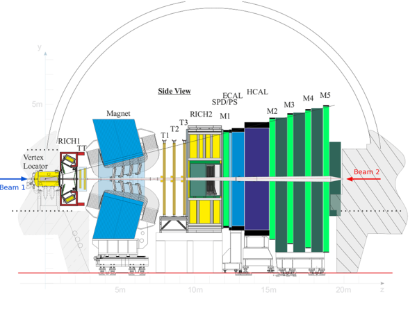
Schematic view of the current LHCb detector. LHC { beam 1 } ({ beam 2 }) enters from the left (right) side of the figure. The labels indicate sub-detectors: vertex locator (VELO), RICH1, RICH2 (ring imaging Cherenkov detectors 1 and 2), TT (tracker Turicensis), T1, T2, T3, (tracking stations 1, 2 and 3), SPD/PS (scintillating pad detector / preshower detector), ECAL (electromagnetic calorimeter), HCAL (hadron calorimeter), and M1, M2, M3, M4, M5 (muon stations 1, 2, 3, 4, and 5) (drawing from Ref. [28]).

Sketch of the VELO sensor positions. The luminous region is schematically depicted with a filled ellipse. Its longitudinal extent, RMS $\sigma = 53\rm mm $, is indicative. Sensors measuring the $R$ ($\phi$) coordinates are shown as blue (red) lines. The LHC beam of ring 1 (2) enters from the left (right) on this sketch. The coordinate system is defined in Sec. 5 (drawing from Ref. [28]).

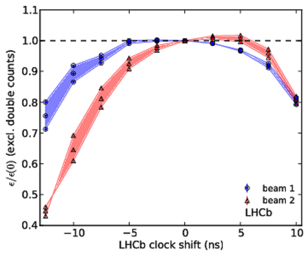
Relative beam-gas trigger efficiency as function of LHCb detector clock shift with respect to the LHC reference timing, (left) including or (right) excluding double-counted beam-gas interaction vertices. The efficiency is shown relative to the value at the nominal clock setting ( i.e. zero shift). The shaded areas indicate the variation between the results for thresholds corresponding to 8 and 12 tracks. The data points, appearing in groups of three, indicate measurements applying the 8, 10 and 12 track thresholds.

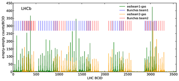
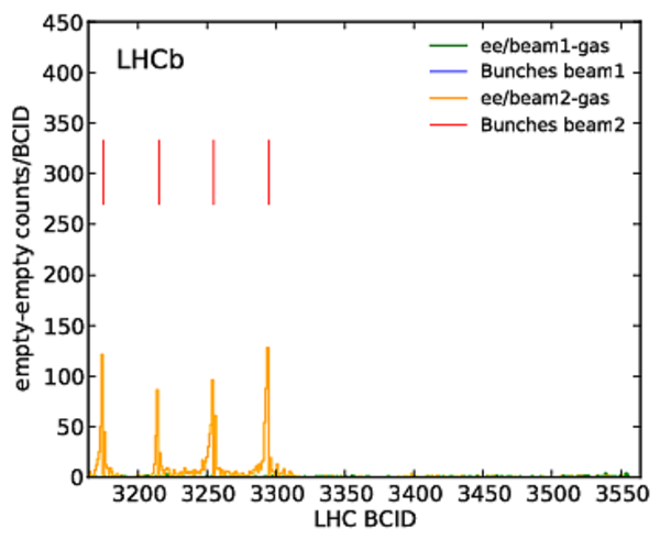
Histogram of ghost charge distribution as a function of LHC bunch slot number (BCID) in fill 2520 for { beam 1 } (green) and { beam 2 } (yellow). The BCID position of nominally filled bunches is indicated as small vertical blue and red lines for { beam 1 } and { beam 2 }, respectively. The ghost charge distribution is shown for the (top) ring circumference and (bottom left) first 400 and (bottom right) last 400 BCIDs. Ghost charges are mostly absent in regions without nominally filled bunches. Note that only $ {\mathsf{ee}}$ BCIDs are displayed.

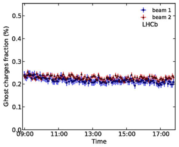
Ghost charge fractions for (left) fill 2855 and (right) fill 3563. Fill 2855 with $\sqrt{s}=8\rm TeV $ shows a constant or slightly decreasing ghost charge fraction throughout the fill lasting about 9 hours. Fill 3563 ($\sqrt{s}=2.76\rm TeV $) shows an important increase of ghost charge over a period of 4 hours.

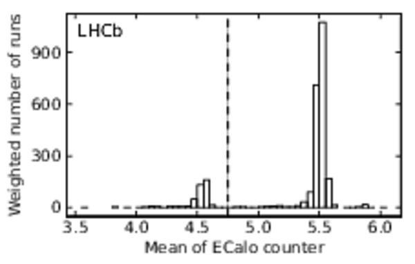
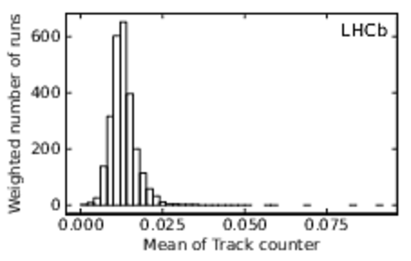
Mean value of (left) ECalo and (right) Track observables in $ {\mathsf{ee}}$ crossings. Each histogram entry represents the average over a run \footnotemark in 2012 and is weighted with the corresponding integrated luminosity. For measurements using the ECalo and Calo observables we discard the runs for which the ECalo pedestal mean is lower than $4.75$ (dashed vertical line).

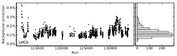
Beam-gas background fraction $\left(-\ln{ {P_0^{\mathrm{ {\mathsf{be}} }}} } -\ln{ {P_0^{\mathrm{ {\mathsf{eb}} }}} }\right)/ {\mu^{}_{\mathrm{\mathrm{vis}}}} $ for the Track observable during the 2012 running period.

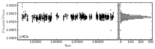
Ratio of the measured $ {\mu^{}_{\mathrm{\mathrm{vis}}}}$ values without (TrackNR) and with (Track) a fiducial volume cut during the 2012 running period. The observed deviation from unity is used as an estimate of the systematic uncertainty due to potentially unaccounted background.

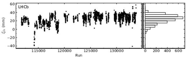
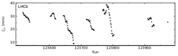
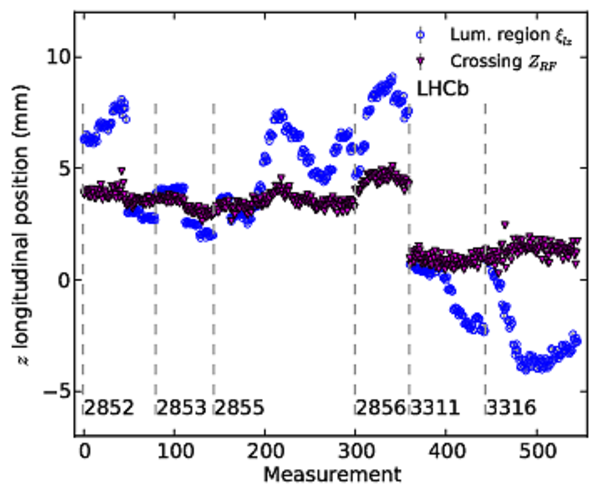
Longitudinal position of the luminous region $\xi_{lz}$ during the 2012 running period. The bottom plot shows a subset consisting of a few fills (distinguished with alternating open and solid markers).

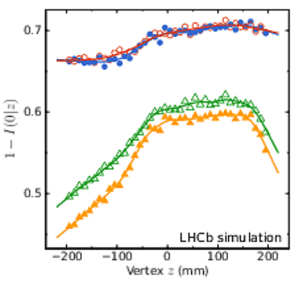
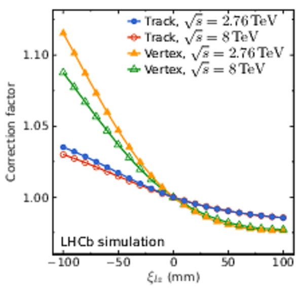
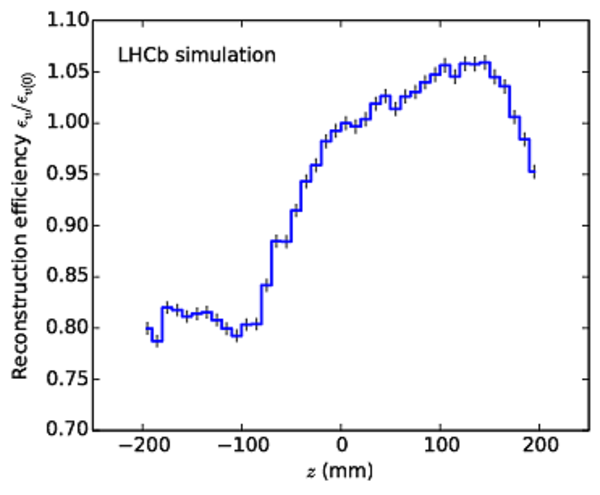
(Left) probability to see an event given an interaction at $z$ and (right) correction factor as function of the longitudinal position $\xi_{lz}$ of the luminous region with size $\sigma_{lz}=50\rm mm $. Only data for one magnet polarity are shown as it is almost identical to that for the other polarity.

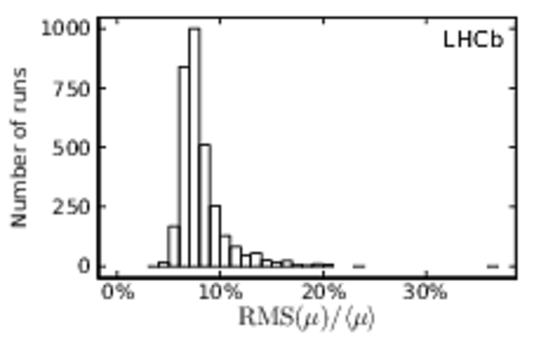
RMS of $ {\mu^{}_{\mathrm{\mathrm{vis}}}}$ across $ {\mathsf{bb}}$ bunch crossings relative to the mean value for the 2012 running period.

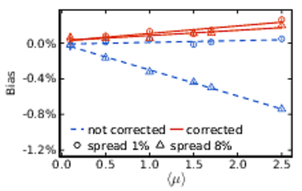
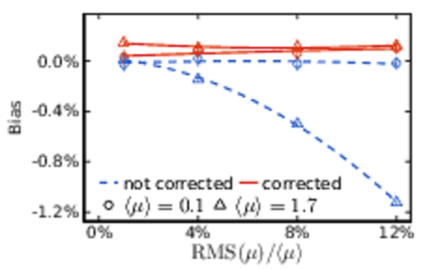
Bias of the estimated number of interactions as function of (left) mean $\mu$ value and (right) relative RMS . The bias is fitted with a straight line and an even quadratic polynomial as function of $\left\langle \mu \right\rangle$ and relative RMS , respectively. A quadratically increasing bias as function of relative RMS is present for large $\left\langle \mu \right\rangle$ values before the correction (dashed blue line). For 2012 data taking conditions, the typical $\left\langle \mu \right\rangle$ for the Track observable is $1.7$ and the typical relative RMS is $8\%$.

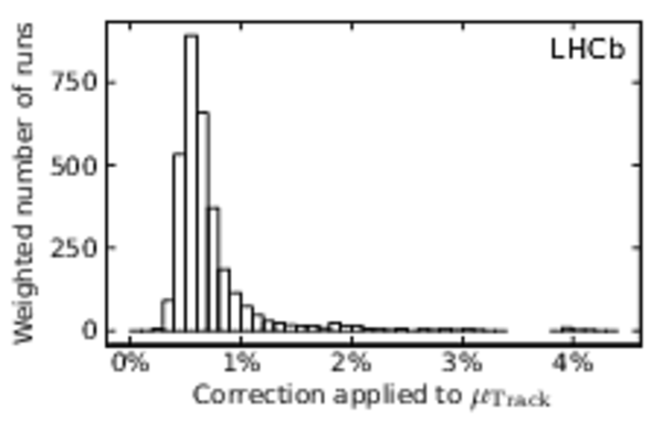
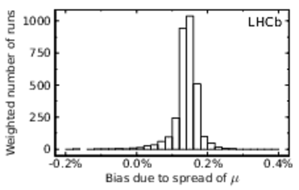
(Left) correction applied to the estimated values of $ {\mu^{}_{\mathrm{Track}}} $ for variations of its value across bunch crossings and (right) residual relative bias of the estimated number of visible interactions after the correction. Each histogram entry represents a run in 2012 and is weighted with the corresponding integrated luminosity.

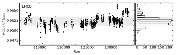
Ratio of the relative luminosities using the Track and the Calo observables during the 2012 running period. Only data for runs that are longer than 30 $\rm min$ are plotted. The variation of the ratio after subtraction of the variation due to statistical fluctuations is shown with a shaded area spanning $\pm 1 \sigma$ around the mean.

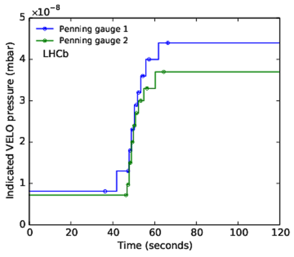
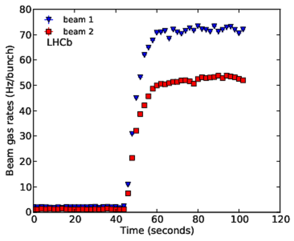
Effect of the gas injection (fill 2520), with (left) the pressure increase in the VELO and (right) the trigger rate increase. The VELO ion pumps are off. The pressure is measured with Penning gauges in the vacuum vessel within $50\rm cm $ of the interaction point. The indicated value when neon is injected is to be multiplied by approximately a factor four to account for the lesser gauge sensitivity to neon gas. The absolute pressure increase cannot be accurately determined as the gas composition in unknown before the start of injection. The beam-gas rate for triggered events increases from about 2 to 72 Hz/bunch for { beam 1 } and 1.3 to 51 Hz/bunch for { beam 2 }.

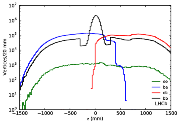
Longitudinal distribution of vertices for the various bunch crossing types acquired in 40 minutes during fill 2852. Crossing types $ {\mathsf{ee}}$ (green), $ {\mathsf{be}}$ (blue) and $ {\mathsf{eb}}$ (red) contain only beam-gas events while the $ {\mathsf{bb}}$ crossing type (black) contains beam-beam vertices in the central region and beam-gas vertices over the whole range. The effect of the prescale factor on the beam-beam interaction rate is visible. The exclusion region of $\pm300\rm mm $ for beam-gas vertices in $ {\mathsf{bb}}$ crossings is visible as the step given by the prescale factor applied to these vertices inside this range.

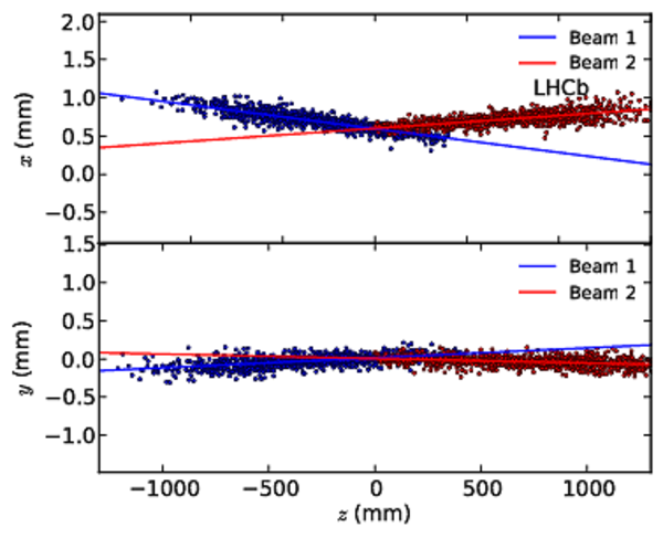
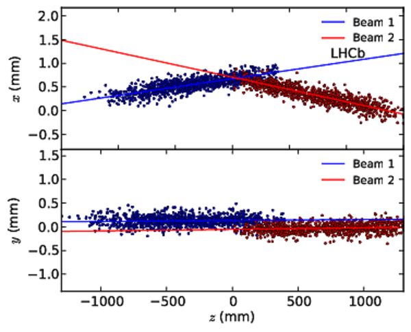
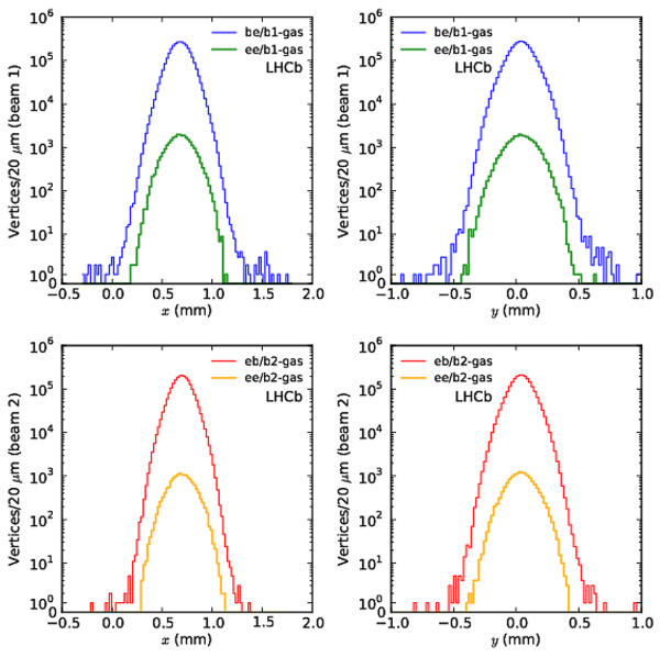
Position of beam-gas vertices projected in the $xz$ and $yz$ planes. The first 1000 vertices per beam are shown. The crossing angles are visible in both planes (left) for fill 2520 and in the $xz$ plane only (right) for fill 2852. The angles are measured by fitting a straight line through all vertices and indicated as solid lines. The beams were offset in the $yz$ plane during this period of fill 2852; { beam 1 } is slightly above { beam 2 } in the $y$ plane (right plot, bottom).

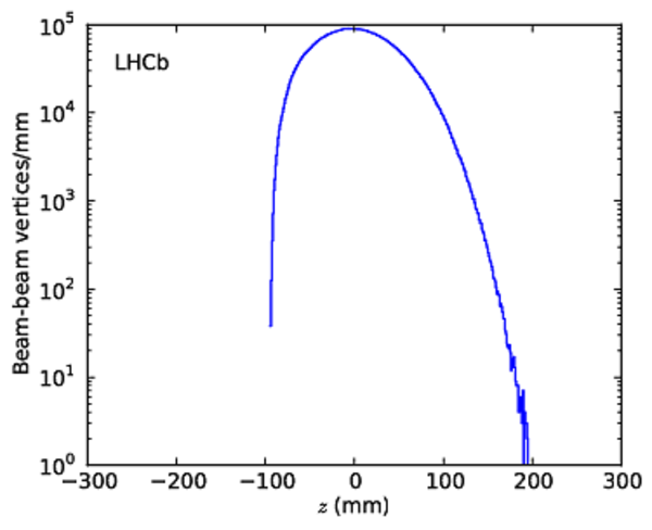
Distributions for beam-beam vertices selected for the resolution measurement with (left) the longitudinal position distribution and (right) the track multiplicity distribution. The requirement to have at least two forward and two backward tracks in each vertex causes the sharp efficiency drop close to $z=-100$ $\rm mm$ . Fill 2520 is selected as example for this figure.

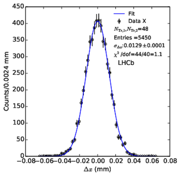
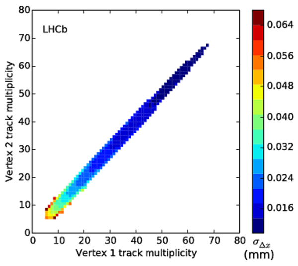
Measurement of the position difference between two sub-vertices from beam-beam interactions (fill 2520). The left-hand panel shows the distribution of distances in $x$ between the two measurements resulting from primary vertex splitting, selecting the case with exactly 48 tracks in both sub-vertices. The data are fitted with a Gaussian function. The right-hand panel shows as a colour code the standard deviation $\sigma_{\Delta v_x}$ of measured distances in $x$ between the two vertices as a function of the vertex track multiplicities. The measured RMS of $0.0129\rm mm $ for two vertices with 48 tracks as shown on the left plot corresponds to the blue square at a multiplicity of 48 for both vertex 1 and vertex 2.

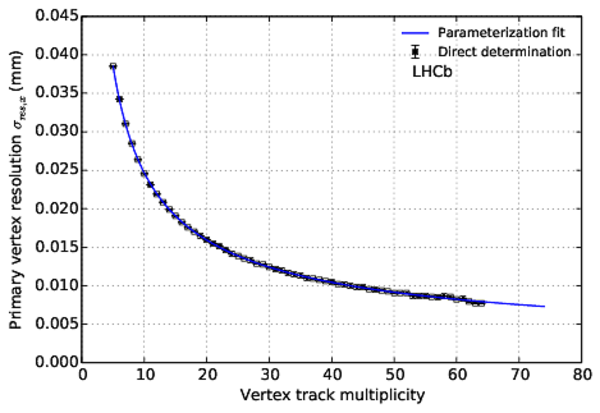
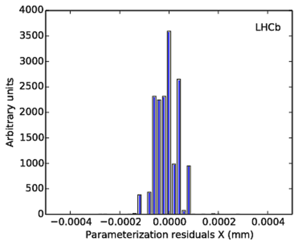
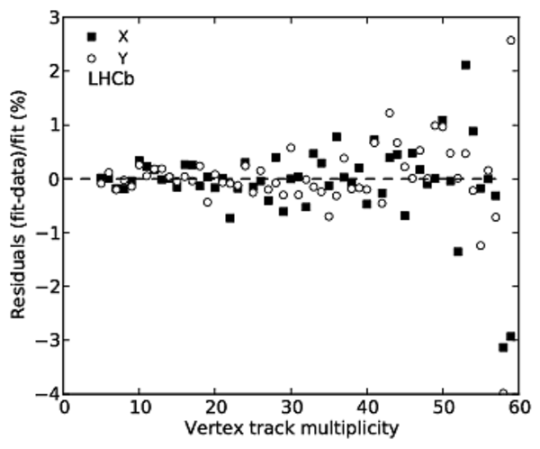
Results of the beam-beam vertex position resolution measurement in fill 2520 with (left) the resolution as a function of the track multiplicity and (right) the distribution of parametrization residuals. The markers in the left plot show the direct determination of the individual resolution for a given vertex track multiplicity for the $x$ coordinate. Results for the $y$ coordinate are similar. The curve shows the results of the resolution parametrization fitted using Eq. 26. In this fill the fit gives the values $A_x = 0.110\rm mm $, $B_x= 0.669$, $C_x= 0.0011\rm mm $, $A_y = 0.101\rm mm $, $B_y = 0.640$, $C_y = 0.0006\rm mm $ for the parameters defined in Eq. 26. The entries in the right plot are weighted by the number of vertices observed with a given vertex track multiplicity.

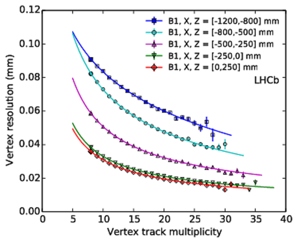
Beam-gas vertex resolution in $x$ as a function of vertex track multiplicity for (left) beam 1 and (right) beam 2 . Fill 2855 is displayed here as an example. Single markers indicate one resolution measurement for a given vertex track multiplicity. The continuous curves indicate the results of the fits using the parametrization in the same $z$ ranges. The statistical uncertainties are shown by error bars. The beam 1 ( beam 2 ) resolution is determined separately in five (four) $z$ regions. The results for the $y$ resolution are similar.

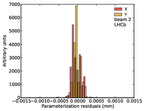
Distributions of residuals between the parametrization and the direct fits for (left) beam 1 and (right) beam 2 . Entries are weighted by the number of vertices observed with a given vertex track multiplicity. Fill 2855 is shown here as example.

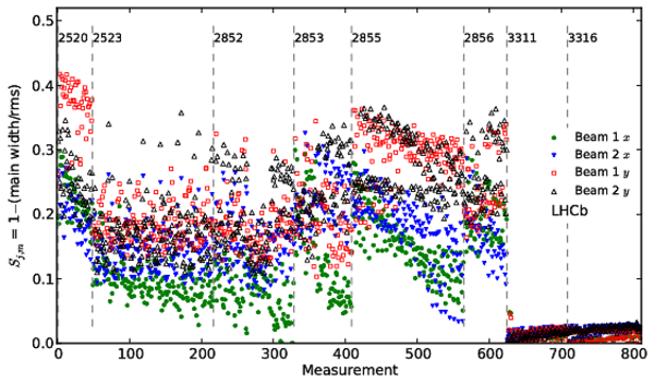
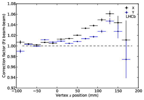
Resolution-deconvolved single beam widths $\sigma_x$ and $\sigma_y$ as a function of $z$ for fill 2520 ($\beta^*=3\rm m $). Values with and without correction factors are shown. Each data point for a given $z$ position is an average of all normalized widths from non-colliding bunches. The curved blue line shows the expected evolution of the beam width due the $\beta^*$ hourglass effect, the shaded blue surface indicates the boundaries corresponding to a 10% uncertainty on $\beta^*$. All points are normalized to the values nearest to $z=0$.

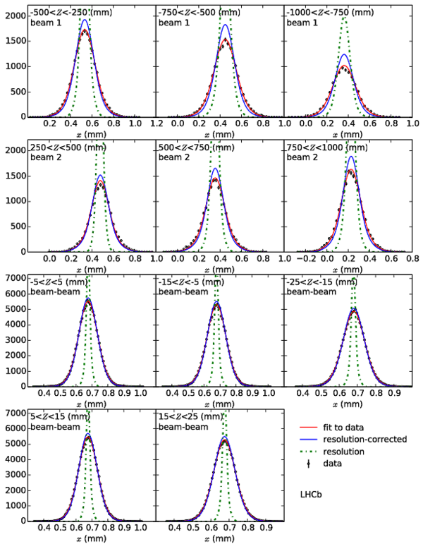
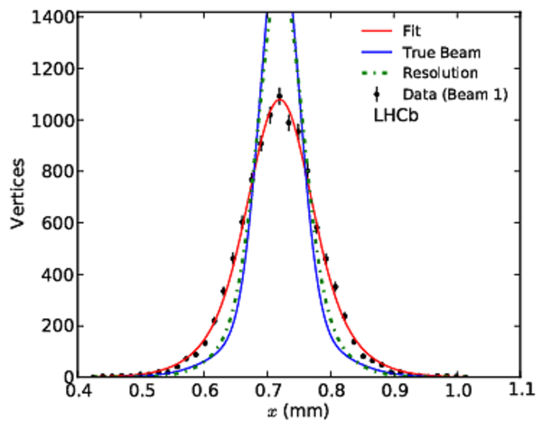
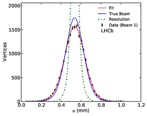
Results of a {1-d} global fit of one colliding bunch pair and for the $x$ coordinate (fill 2852). The first (second) row shows the results of the three { beam 1 } ({ beam 2 }) $z$ slices. The third and fourth row show the results of the central five beam-beam $z$ slices (the remaining 13 slices used in the fit are not shown for better readability). The double Gaussian fit results are shown as solid red lines. The dashed green lines show the effective $x$ resolution functions. The resolution-corrected distributions are shown as solid blue lines.

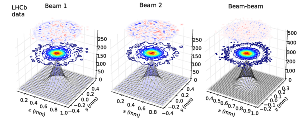
Results of the global {2-d} fit for one bunch pair in fill 2853 as an example, with (left) the central $z$ slice of { beam 1 }, (middle) the central $z$ slice (out of 21) of { beam 2 } and (right) the central $z$ slice of the luminous region. The fit result of the resolution-corrected beam shape is shown as a three-dimensional shape with amplitude indicated on the vertical scale. The data are displayed as a contour plot above the fit result with an arbitrary colour scale with red indicating the maximum. The pulls of the fit are given on the top with a colour scale ranging from $-3$ (dark red) to $+3$ (dark blue).

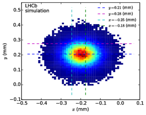
Test of the fit model on simulated data with (left) the transverse view of vertex density of the central $z$ slice at $z=0$ and (right) the comparison of simulated data with predictions for different $x$ and $y$ slices of the luminous region central $z$ region. The colour scale is relative with red indicating the highest number of vertices per bin. The dashed lines indicate the $x$ and $y$ slices in the distribution shown on the right. The markers indicate the simulated data while solid lines show the prediction. Both simulated data and predictions are convolved with the resolution. The beam parameters are simulated with values similar to those observed in the data.

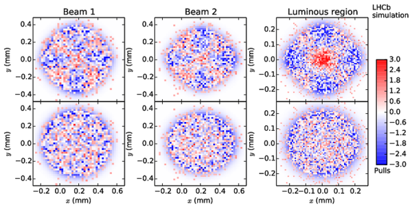
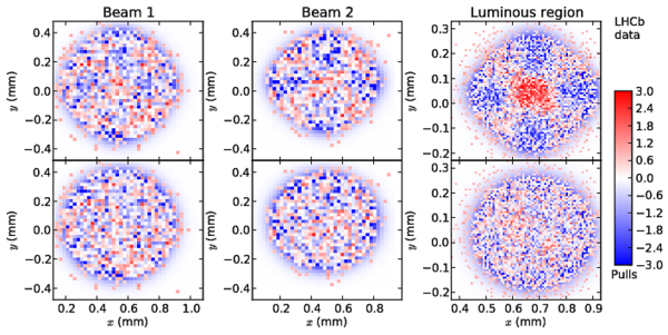
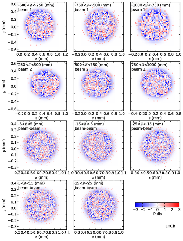
Measurement of transverse beam shape factorizability. The upper six graphs are the results of a simulation. From left to right: fit pulls of a beam $z$ slice for { beam 1 }, { beam 2 } and luminous region. The $z$ slices [$-$500, $-$250] $\rm mm$ for { beam 1 }, [250, 500] $\rm mm$ for { beam 2 } and [$-5$, 5] $\rm mm$ for beam-beam are shown here out of the 24 $z$ slices. The beams are generated assuming non-factorizability, $f_{1,2}=0$; the same dataset is used in both rows but the data are fitted with two different models. Top row: the fit assumes factorizable beams ($f_{1,2}=1$), which is equivalent to the {1-d} model. Bottom row: fit with the additional beam factorizability parameters $f_{1,2}$. The fit converges to the correct parameter valuess $f_{1,2}=0$. The lower six graphs are the results of a fit to data (fill 2855, BCID 1335), which converges to non-factorizable beam shapes in this example. \\ \\

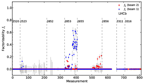
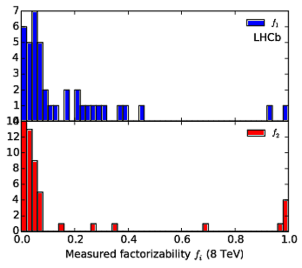
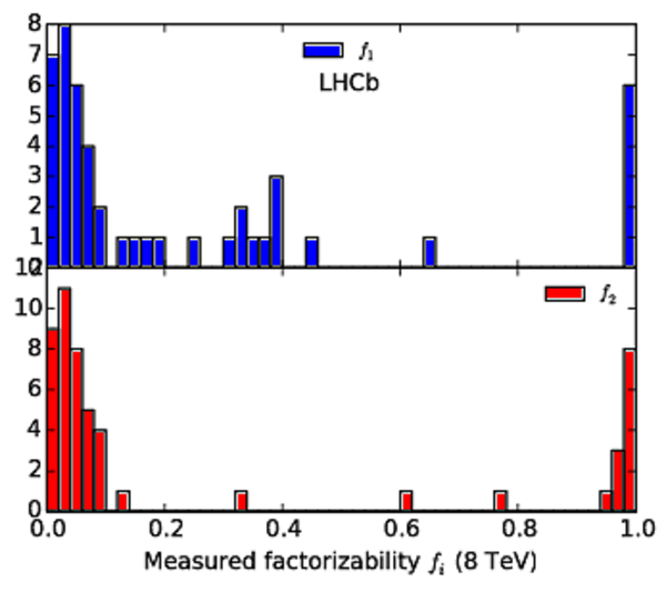
Fit results for factorizability parameters $f_{1,2}$ for (left) the simulation and (right) all measurements performed in 2012 at $\sqrt{s}=8\rm TeV $. In the simulation, different double-Gaussian beam parameters were used and the values of $f_{1,2}$ were set to 0 or 1. For the data, only bunch pairs with a double Gaussian strength $S_{j,m}>0.02$ and with a fit uncertainty on the factorizability parameter of $\delta(f_j)<1$ are displayed. The top (bottom) panels refers to { beam 1 } ({ beam 2 }).

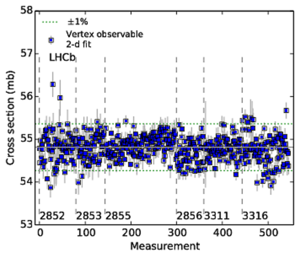
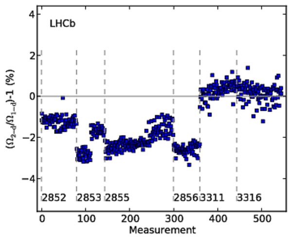
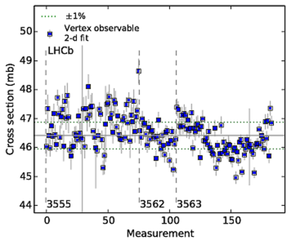
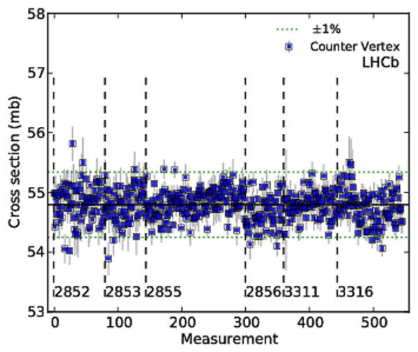
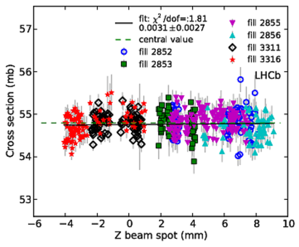
Cross-section results for head-on beams with $\beta^*=10$ m at $\sqrt{s}=8$ TeV using the Vertex observable, (left) the {2-d} fit and (right) the relative difference between the {2-d} and {1-d} fit. Each data point is a cross-section measurement from a colliding bunch pair using integrated data over about 20 minutes. The measurements are sorted by time and BCID. The fills are indicated in the figure and are separated by dashed vertical lines. Two dotted horizontal lines indicate a $\pm 1\%$ deviation from the central value. The error bars show the statistical uncertainties of the overlap integral.

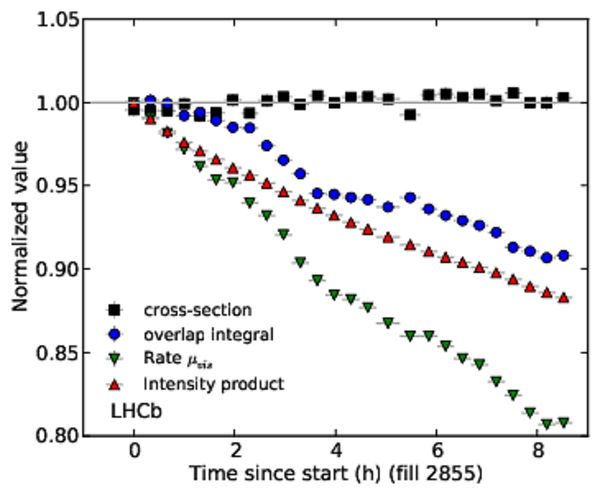
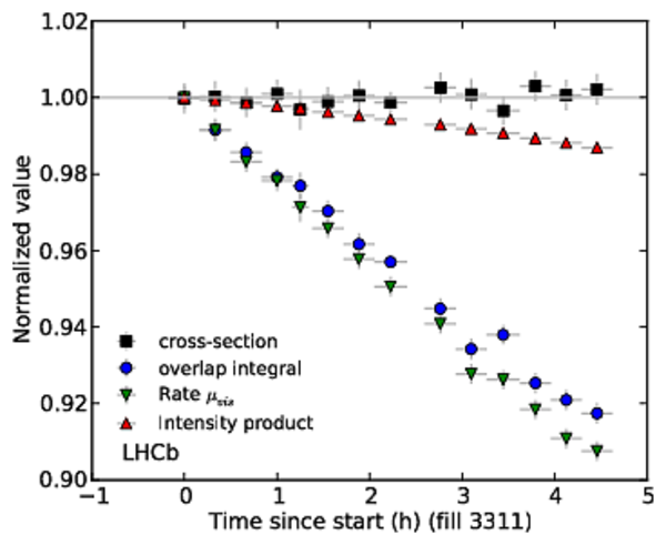
Evolution of normalized cross-section and related values for a colliding bunch pair for BCID 1335 of (left) fill 2855 and (right) of fill 3311. The cross-section values are normalized to their average while other parameters are normalized to the first data point. Fill 2855 lasted more than eight hours with a beam intensity product decrease of about 10%. Fill 3311 lasted about 4h30 with a beam intensity product decrease of less than 2%; in this fill the luminosity reduction is mostly caused by emittance growth.

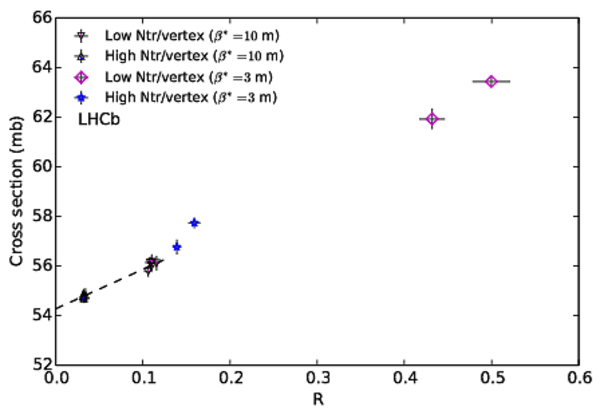
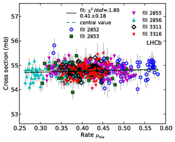
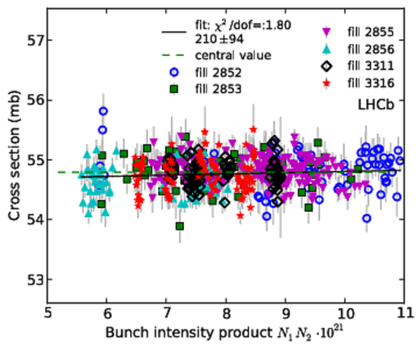
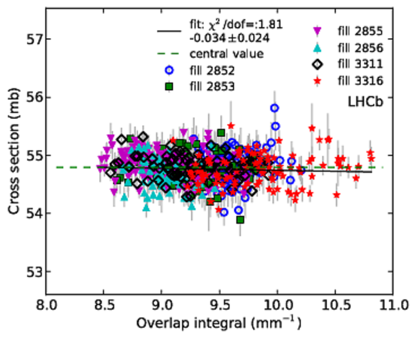
Illustration of the evaluation of the systematic uncertainty due to the beam-beam resolution. Measured visible cross-section values for different event samples are shown as a function of $R$. The $R$ parameter is calculated with Eq. 35. Each data point is an average of all measurements from a fill. The error bars are the RMS of the cross-section and $R$ values per fill. Plain markers are measurements performed with $\beta^*=10\rm m $ (6 fills) and open markers are performed with $\beta^*=3\rm m $ (2 fills). The samples with $R \approx 0.5$ are selected to enhance the effect of the resolution. The dashed line visualizes the determination of the systematic uncertainty as described in the text.

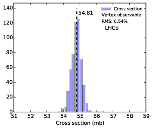
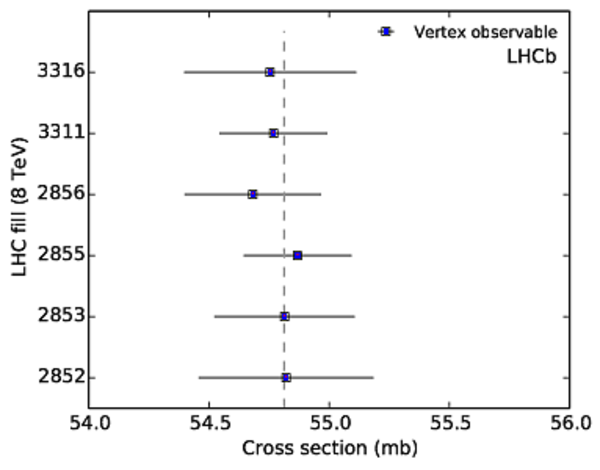
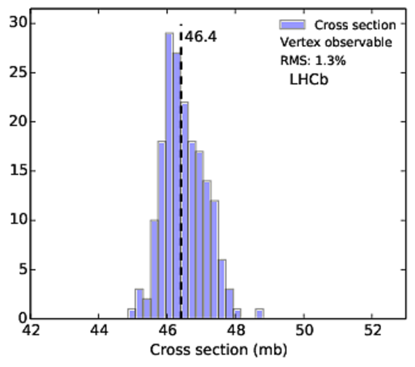
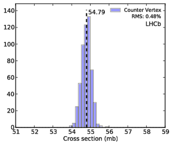
Overview of cross-section measurements for head-on periods in fills with $\beta^*=10\rm m $ at $\sqrt{s}=8\rm TeV $ with (left) the histogram combining all data from Fig. 29 and (right) the central value of cross-sections averaged per fill. The dashed vertical line indicates the median value of all measurements. The error bars indicate the standard deviation of all measurements from a fill. The statistical uncertainty of each average is smaller than the marker size.

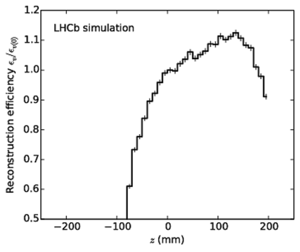
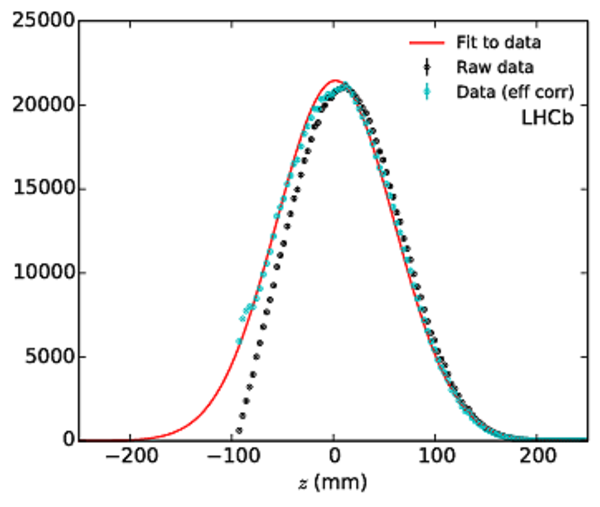
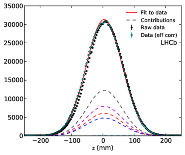
Determination of the bunch length of a colliding bunch pair with (left) the vertex reconstruction efficiency as function of $z$ and (right) the fit to the longitudinal vertex distribution after efficiency correction. The statistical uncertainty on the corrected points is dominated by the limited amount of simulated data. This component of the uncertainty is not shown in the right-hand plot. The data are selected requiring vertices with at least two forward and two backward tracks. The efficiency is normalized to the value at $z=0$ to keep similar amplitudes between the raw and corrected data; the absolute scale of the correction does not change the fit results. This example displays data for BCID 1335 in fill 2855. The raw data (black dots) show the distortion resulting from the requirement of having at least two tracks in both directions.

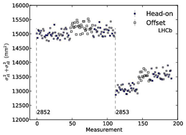
Measurement of convolved bunch length $\sigma_{z1}^2+\sigma_{z2}^2$ with displaced beam during fills 2852 and 2853. The fills are indicated in the plot and separated by a dashed vertical line. The measurements are sorted by time and BCID. About 3.5 hours separate the first head-on period in fill 2853 from the period with offset beams explaining the higher values of the bunch length observed during that period. The next head-on period follows the period with offset beams without time interval.

Cross-section results with head-on beams with $\beta^*=10$ m at $\sqrt{s}=2.76$ TeV for the Vertex observable, with (left) the individual measurements and (right) the histogram of the values. The individual measurements are made per colliding bunch pair and 20 minutes time integration and are sorted by time and BCID. The different fills are separated by a dashed vertical line in the figure. Two dotted horizontal lines show the $\pm1\%$ deviation from the central value. The measurement spread has a 1.3\% RMS . The median value is indicated by a dashed vertical line in the right-hand plot.

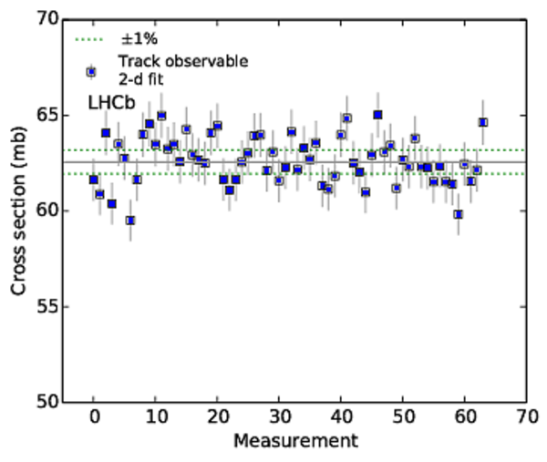
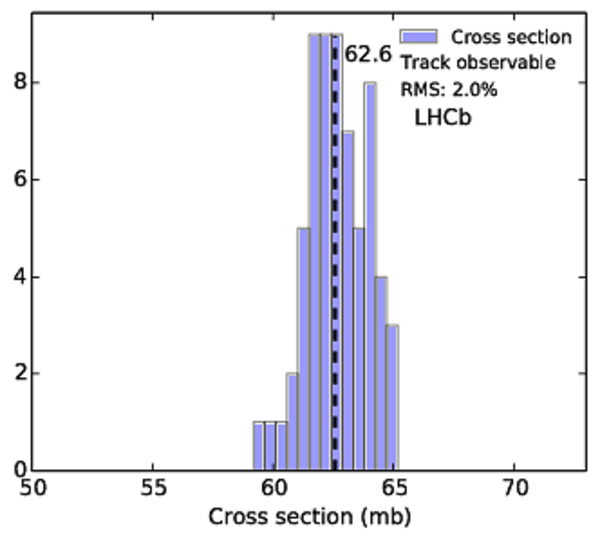
Cross-section results at $\sqrt{s}=7$ TeV in 2011 for the Track observable, with (left) the individual measurements and (right) the histogram of the values. The individual measurements are made per colliding bunch pair, for a one hour integration time, and are sorted by time and BCID. The different fills are separated by a dashed vertical line in the figure. Two dotted horizontal lines show the $\pm1\%$ deviation from the central value. The measurement spread has a 2.0\% RMS . The median value is indicated by a dashed vertical line in the right-hand plot.

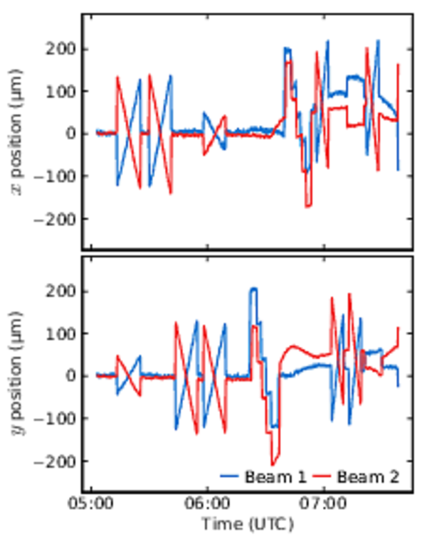
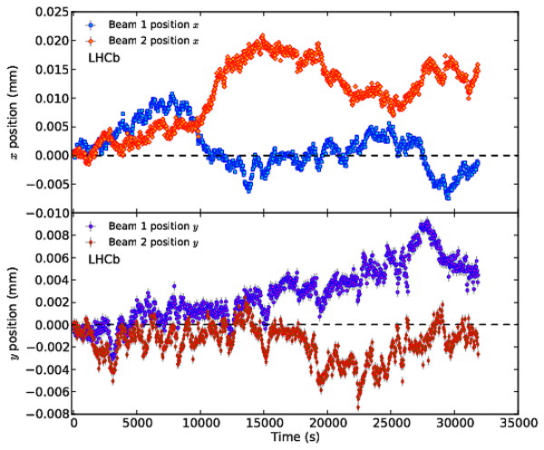
Beam positions recorded with the LHC beam position monitors around the LHCb interaction point in the (left) April and (right) July VDM sessions. The initial values are set to zero. The top (bottom) panel shows horizontal (vertical) positions. In all scans the beams are moved symmetrically. The beam movements around 6:30 (22:40) in April (July) correspond to the length scale calibration by the constant separation method.

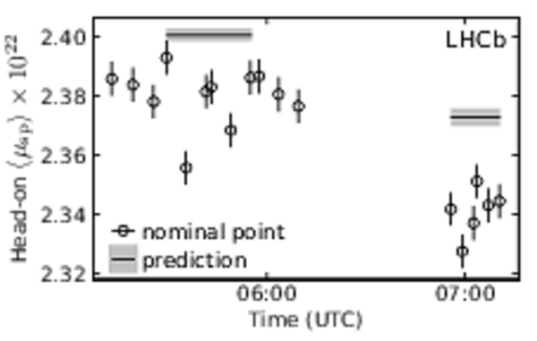
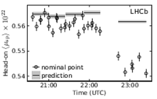
Evolution of the specific average number of interactions per crossing ($ {\mu^{}_{\mathrm{sp}}} $) at the nominal head-on beam positions during the (left) April and (right) July VDM sessions. In each scan the nominal point was measured three times and the average over bunches is plotted with open markers. The value at the actual zero beam separation is predicted for each scan pair (excluding offset and tilted scans) and shown with a horizontal band. The difference with respect to the values at zero nominal separation is due to the working point not being exactly at zero beam separation. The beam positions were not re-optimized during the sessions.

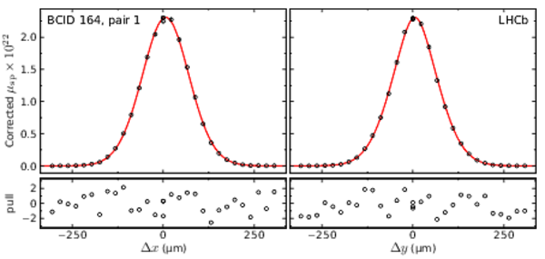
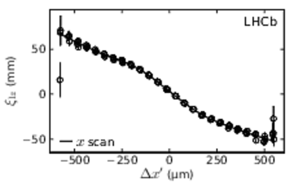
Fit of VDM profiles for a single bunch and scan pair in the (top) April and (bottom) July VDM sessions. The left (right) panels show data and fit predictions corresponding to the $x$ ($y$) scan. The data points are represented with circles, while the fitted curve is shown as a solid line. The error bars are smaller than the symbol size. The fit pulls are displayed below each fit projection and show no systematic structure. There are three data points at $\Delta m = 0$ as the nominal point was measured three times for each scan.

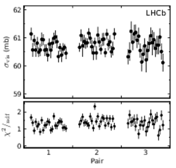
(Top) measured cross-section values and (bottom) the corresponding values of $\chi^2/\mathrm{ndf}$ for all bunch pairs and for non-offset scan pairs in the (left) April and (right) July VDM sessions. Measurements within one scan pair are separated from the rest by a larger distance.

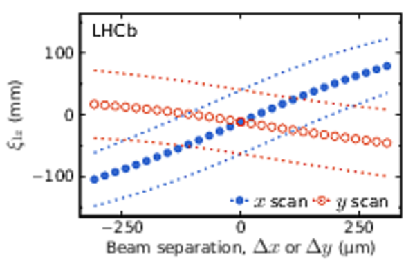
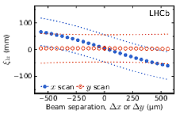
Luminous region longitudinal position and size as function of beam separation for a scan pair in the (left) April and (right) July VDM sessions. The values for other scan pairs are similar. Markers indicate the mean while the bands between dotted lines contain 68% of the vertices. In April, the luminous region moves in both horizontal and vertical scans because of the crossing angle configuration. The inversion of the slope in the horizontal scan is due to the change of sign of the crossing angle between the two sessions.

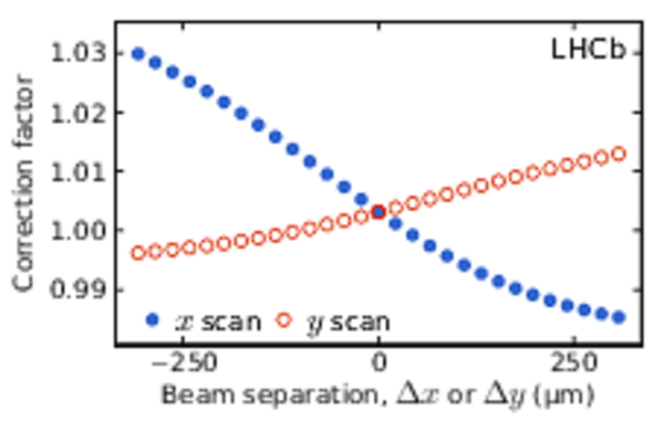
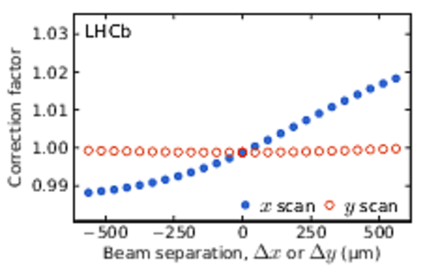
Efficiency correction factors for the Track observable for a scan pair in the (left) April and (right) July VDM sessions. The values for other scan pairs are similar.

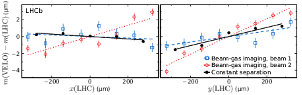
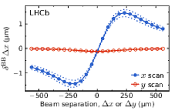
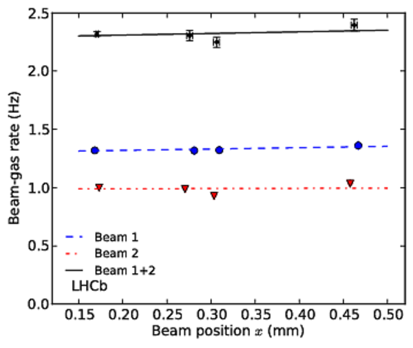
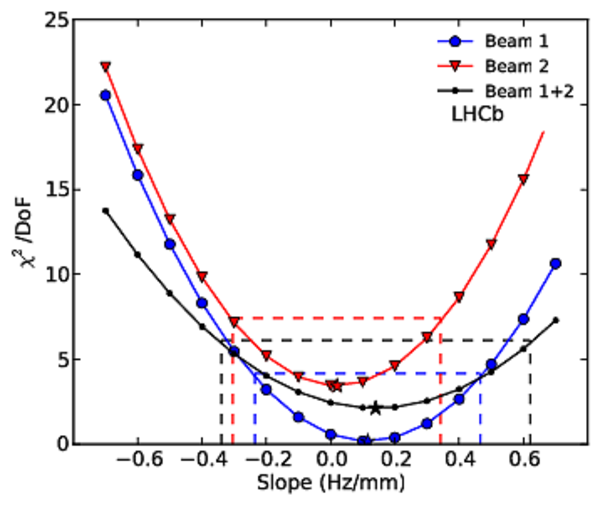
Length scale calibration fits in the (left) $x$ and (right) $y$ axis in the July VDM session. The fitted intercepts are subtracted from both the fit curves and the data points as they have no significance. Each data point is an aggregate of the measurements from 16 colliding bunch pairs for the constant separation method and 35 individual bunches for the BGI method. The fit slope obtained using the constant separation method (solid line) should be compared with the average of the slopes obtained with the BGI method (dashed and dotted lines).

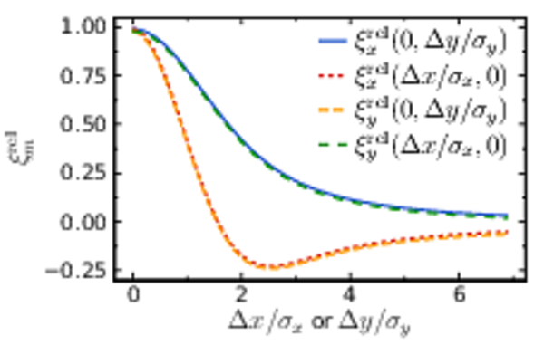
Relative change of the beam-beam parameter as function of beam separation. The values are obtained using a simulation of the machine optic elements.

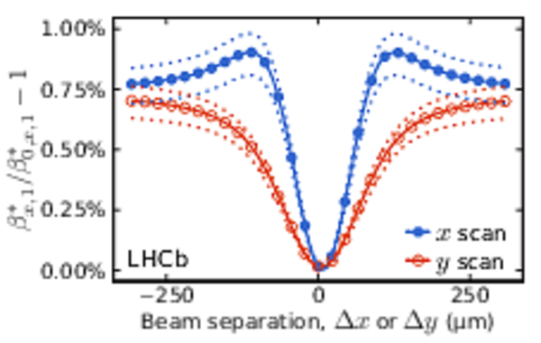
Relative $\beta^*$ change for beam 1 in the $x$ axis as as function of beam separation for a scan pair in the (left) April and (right) July VDM sessions. The values for other scan pairs are similar. The values for beam 2 are similar owing to similar bunch intensities. The values for the $y$ axis are also similar with $x$ and $y$ scans exchanged. The markers and the solid line represent the average, while the dotted lines correspond to the extremes among colliding bunches. The reference $\beta^*$ is chosen such that the relative change is zero at the separation corresponding to maximum luminosity.

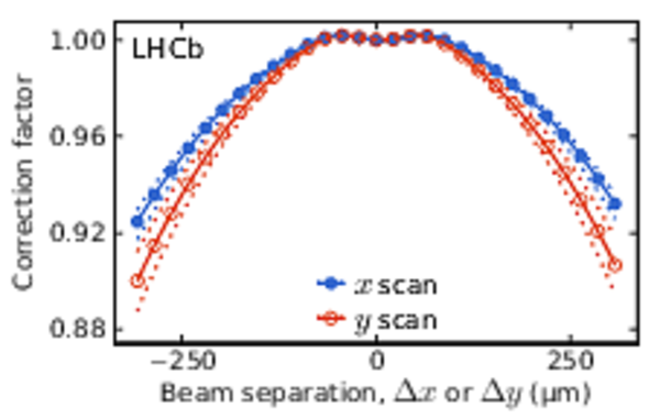
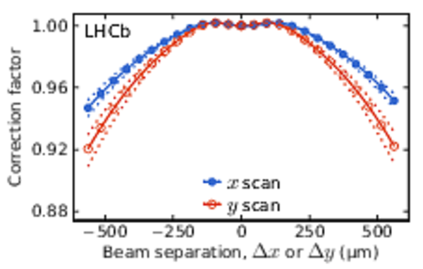
Rate correction factor for the dynamic beta effect for a scan pair in the (left) April and (right) July VDM sessions. The values for other scan pairs are similar. The markers and the solid line represent the average, while the dotted lines correspond to the extremes among colliding bunches. Owing to the dynamic $\beta$ effect, the $\beta$'s and thus the beam sizes depend on the beam separation. To take this into account, the effect on the luminosity is compensated by multiplying the observed rates with the correction factors.

Correction to the nominal separation in the $x$ axis for beam-beam-induced orbit shift for a scan pair in the (left) April and (right) July VDM sessions. The values for other scan pairs are similar. The values for the $y$ axis are similar with $x$ and $y$ scans exchanged. The markers and the solid line represent the average, while the dotted lines correspond to the extremes among colliding bunches.

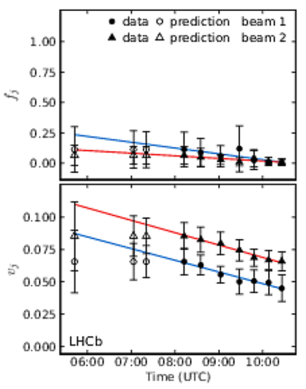
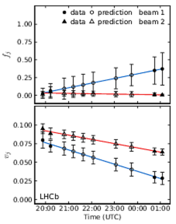
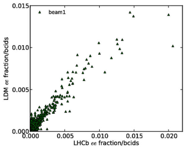
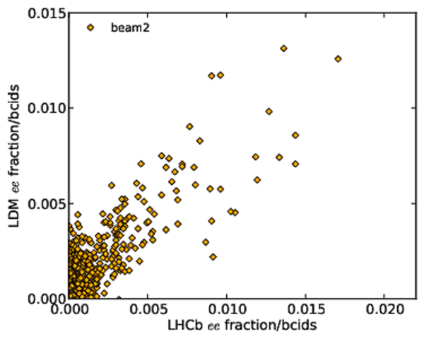
Values of the (top) factorizability parameter $f_j$ and (bottom) generic factorizability measure $v_j$ in the (left) April and (right) July VDM sessions. The filled markers and the corresponding error bars indicate the average and the RMS of BGI measurements for individual bunch pairs. In the case of the July scans, BGI measurements are available before and after the VDM session, thus the values are linearly interpolated to obtain predictions at the time of VDM scan pairs (open markers). For April, as BGI data are only available after the VDM scans, the closest data points are used as a prediction, while the difference to the linear extrapolation is added in quadrature to the uncertainties. The trend of the generic factorizability measure shows that beam distributions become more factorizable as function of time.

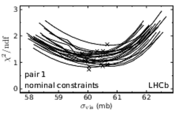
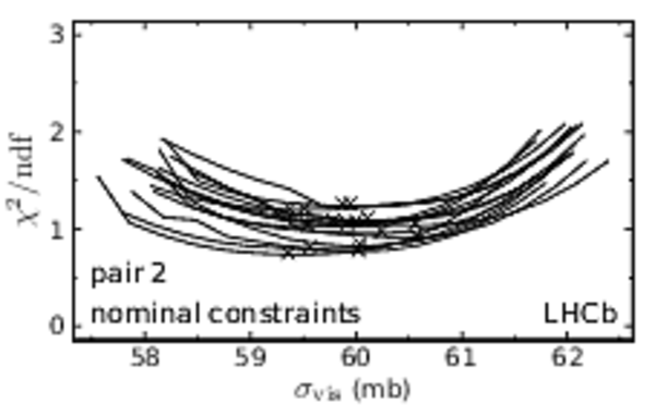
Examples of the constrained fit $\chi^2/\mathrm{ndf}$ profiles as function of $\sigma_\mathrm{vis}$ for (left) scan pair 1 in April and (right) scan pair 2 in July. Each curve corresponds to one bunch pair. The values of $\sigma_\mathrm{vis}$ obtained with direct fitting are shown with cross markers.

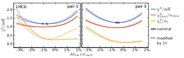
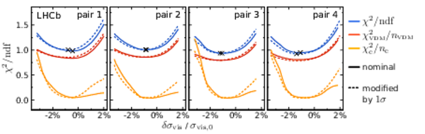
Average $\chi^2/\mathrm{ndf}$ profiles as function of the relative difference to the baseline cross-section for the reference scan pairs in (top) April and (bottom) July shown with the top pair of lines (blue). The profiles corresponding to the nominal and modified constraints are shown with solid and dashed lines, respectively. The minima of the $\chi^2/\mathrm{ndf}$ profiles are marked with a cross. The contribution of the VDM data, $\chi^2_{ VDM}$, normalized to the number of points in the VDM scan pair $n_{ VDM}$ is shown with the middle pair of lines (red). The contribution of the constraints, $\chi_\mathrm{c}^2$, normalized to the number of constraints $n_\mathrm{c}$ is shown with the bottom pair of lines (yellow).

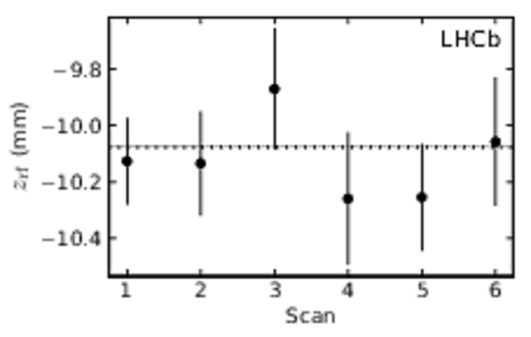
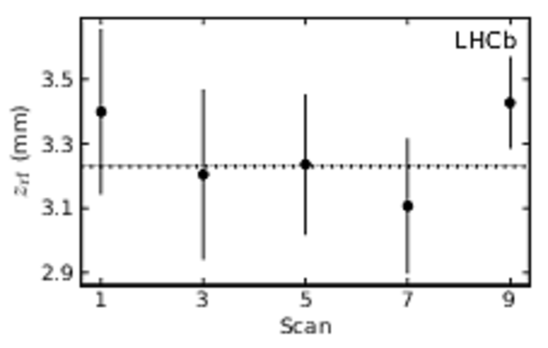
Values of $z_{\rm rf}$ in (left) April and (right) July scans. The implied assumptions are that $z_{\rm rf}$ does not change and there is no orbit drift during a scan pair. No measurements are performed for offset scans. The deviations of the measurements from the weighted average (horizontal dotted line) are not statistically significant.

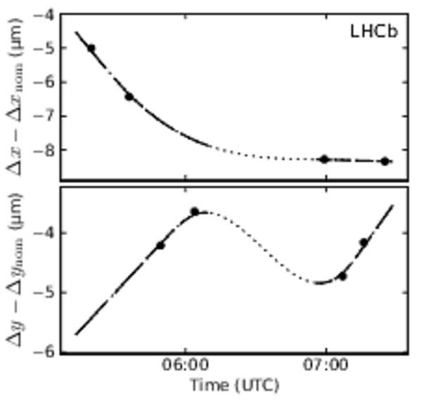
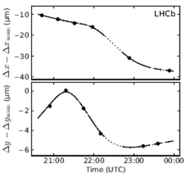
Estimated "slow" drift of the beam separation in the (left) April and (right) July VDM sessions. The nominal separation where the luminosity is maximal gives a single estimate per scan of the drift in the corresponding direction (circles). The uncertainties are smaller than the marker size. The data for each coordinate are fitted with a smooth function (curve) and a prediction is made at each step of every scan (solid curve).

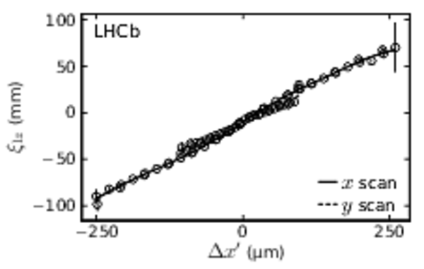
Longitudinal position of the luminous region as function of separation in the crossing plane for reference scans in the (left) April and (right) July VDM sessions. It is assumed that there is no significant orbit and $z_{\rm rf}$ drift during the reference scans. The data for each scan direction are fitted with a smooth function. In July the crossing plane is orthogonal to the $y$ axis, thus $\xi_{lz}$ is not expected to change during the $y$ scans and the data are omitted. The non-linearity of the curves is due to second order effects, which are not expected for pure Gaussian beams.

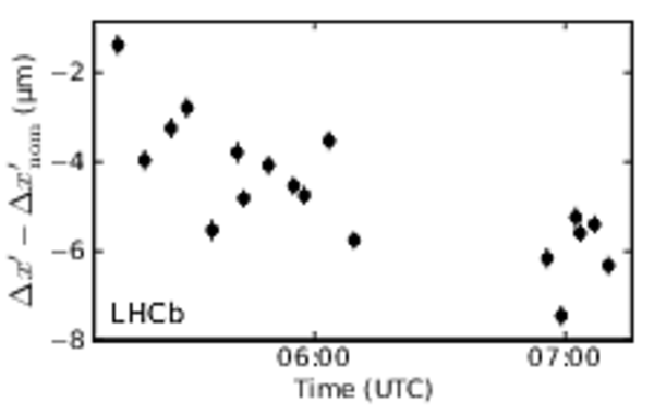
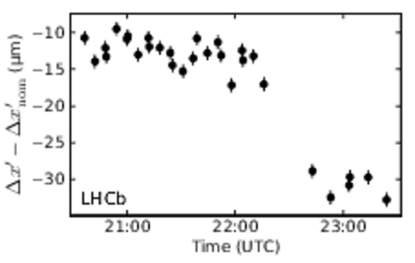
Estimated drift of the beam separation in the crossing plane $\Delta x '$ in the (left) April and (right) July VDM sessions. The drift is estimated only for each nominally head-on step.

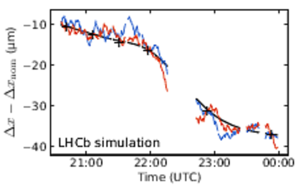
Two example simulations of the beam separation drift in the $x$ coordinate for the July VDM session. The separation drift is modelled with a Brownian motion that is constrained to the measured slow component of the drift (smooth black line) at the measurement points (crosses).

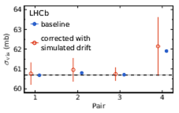
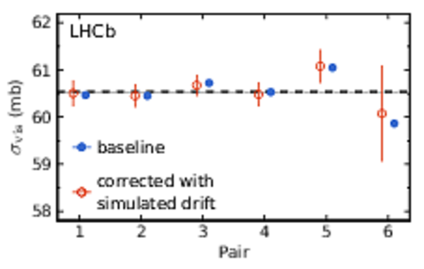
Cross-section bias caused by beam orbit drifts in the (left) April and (right) July VDM sessions. The baseline cross-section for each pair is shown with a solid circle and the average calibration cross-section (using the reference pairs) is shown with a horizontal dashed line. The average biased cross-section obtained with simulation of the beam drifts is shown with open circles. The error bars indicate the RMS of the biased cross-section of 400 independent simulations. The larger error bars for the offset scan pairs indicate that they are more sensitive to random drifts.

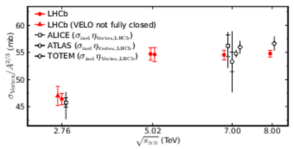
Measurements of the visible cross-section for the Vertex observable as function of centre-of-mass energy. The measurement at 2.76 $\mathrm{ Te V}$ [51] performed using the VDM method (solid triangle) is corrected for the reduced efficiency due to the VELO being not fully closed. The visible cross-section for proton-lead collisions at 5 $\mathrm{ Te V}$ is scaled by $A^{-2/3}$. A comparison is made with the luminosity-independent measurements of the $pp$ inelastic cross-section by the TOTEM collaboration [52,8] at 7 and 8 $\mathrm{ Te V}$ , with direct measurements by the ALICE [53] and the ATLAS [54] experiments, and with a measurement by ATLAS from elastic $ pp$ scattering [9]. The measurements from other experiments are scaled with the LHCb efficiency for inelastic events $\eta_\mathrm{ Vertex,LHCb}$ , obtained from simulation. The uncertainties of the direct measurements from ALICE and ATLAS are dominated by the extrapolation of the visible cross-section to the total inelastic cross-section and are not to be compared with the uncertainties of the LHCb measurements. The tick marks represent the uncertainty due to the luminosity calibration only. Data points at the same centre-of-mass energy are displaced horizontally for clarity.

Animated gif made out of all figures.

Dedicated LHC calibration fills during which LHCb performed the luminosity calibrations described in this paper or ghost charge and beam size measurements for other LHC experiments. In most calibration measurements the number of bunches per beam was the same for { beam 1 } and { beam 2 }. For the $p$Pb and Pb$p$ fills where this was not the case two numbers are given, the first for the number of { beam 1 } bunches, the second for the number of { beam 2 } bunches. The number of colliding bunches at LHCb is indicated in parentheses (fifth column). Half crossing angles $\phi_x$ and $\phi_y$, and $\beta^*$ are given as nominal values. The VELO vacuum state during BGI measurements is indicated in the column "Gas injection". A state "off" means that gas injection was turned off and the VELO ion pumps were turned off, which resulted in a residual vacuum pressure about a factor four higher than nominal. A state "on" indicates that neon gas was being injected into the beam vacuum. During VDM measurements the state was always "off".

Relative beam-gas trigger efficiency for the ghost charge measurement assuming a constant charge distribution within a bunch slot.

Measurements of ghost charge fractions for all luminosity calibration fills in 2011, 2012 and 2013. The systematic uncertainty is assumed to be fully correlated between the two beams. Therefore, the final systematic uncertainty on the beam intensity product due to the ghost charge correction is a linear sum of the ghost charge systematic uncertainty of each beam. Proton-lead fills were acquired without neon gas injection and have a larger statistical uncertainty. For fill 3542 the ghost charge was only measured using the LHC LDMs.

Relative uncertainties (in percent) on colliding-bunch population products for all relevant fills.

Definition of luminosity observables used in the analysis. The fiducial volume used here is a cylinder of radius $< 4\rm mm $ around the $z$ axis and bound by $|z|<300\rm mm $. It is used to cut either on the point of closest approach of a track relative to the $z$ axis or on the position of a vertex.

Top: systematic uncertainties of the relative luminosity measurement (in %). Bottom: integrated effect of the applied corrections (in %).

Relative systematic uncertainties on the reference cross-section for the BGI calibrations at $\sqrt{s}$ values of 8, 7 and 2.76 $\mathrm{ Te V}$ (in %). The uncertainties are divided into groups affecting the measurement of the overlap integral (Sec. 6), the bunch population product (Sec. 3) and the rate measurement (Sec. 4).

Parameters of VDM scans. The scan pairs marked with an asterisk are not used in the determination of the central value of the cross-section (as explained in the text). The step duration indicates the period of stable conditions available for the measurement.

Length scale calibration constants. All uncertainties are statistical.

Uncertainties of input parameters to the correction for beam-beam effects. All quantities are correlated between axes. The quantities $\beta^* _{m,j}$ and $Q_{m,j}$ are not correlated between the two beams.

Effect of corrections on the result of the VDM scan calibrations at $\sqrt{s_{ {\it NN}}}$ values of 8, 7 and 5 $\rm TeV$ (in %). To obtain the effects, each correction is excluded, the fits are redone and the result is compared with the baseline.

Individual calibration results and average of the $8\rm TeV $ $pp$ VDM scan sessions. The part of the relative uncertainty that is correlated between the calibrations is shown in the fourth column. The weights used to obtain the average are given in the last column.

Relative systematic uncertainties on the reference cross-section for the VDM calibrations at $\sqrt{s_{ {\it NN}}}$ values of 8, 7 and 5 $\mathrm{ Te V}$ (in %). The uncertainties are divided into groups affecting the description of the VDM profile (Secs. 7.5--7.8), the measurement of the rate (Sec. 7.4) and the bunch population product measurement (Sec. 3). The fourth (eight) column indicates whether the uncertainties are correlated between the two $pp$ calibrations at $\sqrt{s}=8\mathrm{ Te V} $ (the $p$Pb and Pb$p$ calibrations). Empty cells indicate that the corresponding source is not applicable or the uncertainty is negligible. For the $p$Pb and Pb$p$ calibrations, the uncertainties due to scan variation and drift, and non-reproducibility cannot be estimated separately as only two VDM scan pairs per calibration were performed.

Systematic uncertainties of the BGI and VDM methods for $ pp$ interactions at $8\rm TeV $. The fourth column indicates whether the uncertainties are correlated between the two calibrations. All values are given in %.

Results of the luminosity calibration measurements. The total uncertainty on the luminosity calibration (last column) is the sum in quadrature of the absolute calibration uncertainty (fourth column) and the relative calibration uncertainty (fifth column). The weights used to obtain the average absolute calibration at 8 and 7 $\mathrm{ Te V}$ ( $ pp$ ) are given in the third column. The part of the uncertainty that is correlated between VDM and BGI calibrations is shown in parentheses (fourth column).

Supplementary material full pdf

This ZIP file contains supplemetary material for the publication LHCb-PAPER-2014-047. The files are: supplementary.pdf : An overview of the extra figures *.pdf, *.png : The figures in variuous formats