
Jet substructure at very high luminosity
Pythia 8 [1] samples produced with the Phase II LoI baseline tracker are used [2]. Samples with a mean number of interactions per bunch crossing (mu) of 0, 80, 140, 200 and 300 are used. Calorimeter noise thresholds are adjusted for each mu. Except for mu=0 where the calorimeter noise is optimised for mu=30 as in 2012 data. The pileup suppression uses the event-by-event median pT density (rho) and the jet area [3]. Rho is calculated using kt R=0.4 jets reconstructed from locally calibrated (LCW) topoclusters [4] within |eta| <2.0. The density calculation is with respect to the Voronoi area of the jets. Trimming [5] with parameters fcut>5% and Rsubjet = 0.3 is used. The pileup correction is made to the subjets only before their pT is calculated for the trimming procedure. No systematic uncertainties are included in these plots.Plots
| Distributions of jet splitting scales [1] for the leading pT anti-kt trimmed R=1.0 jet in Z-> ttbar (mZ=2 TeV) events with mean number of interactions per bunch crossing (mu) of 80 (red closed squares),140 (red open squares), 200 (black open crosses) and 300 (black closed crosses). Jets with |eta|<1.2 and 0.5 TeV<pT<1 TeV are used. The left plot shows the first splitting scale sqrt(d12) and the right plot corresponds to the second splitting scale sqrt(d23). The peak at low sqrt(d23) corresponds to jets that do not fully contain all the hadronic decay productions of the top quark. This peak get smeared with increased pile-up and therefore convoluted with the peak at higher sqrt(d23). | 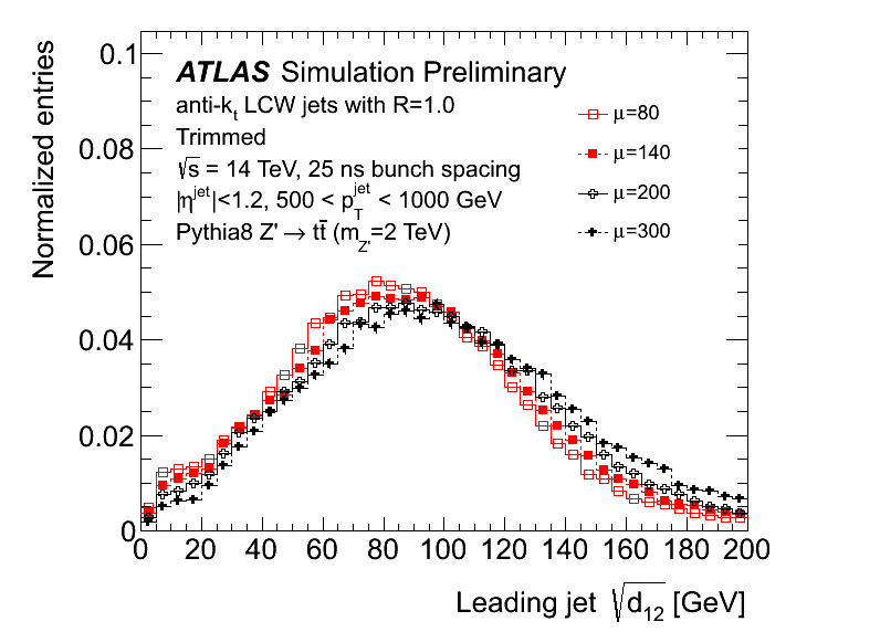 [pdf] [eps] |
| Distributions of jet splitting scales [1] for the leading pT anti-kt trimmed R=1.0 jet in Z-> ttbar (mZ=2 TeV) events with mean number of interactions per bunch crossing (mu) of 80 (red closed squares),140 (red open squares), 200 (black open crosses) and 300 (black closed crosses). Jets with |eta|<1.2 and 0.5 TeV<pT<1 TeV are used. The left plot shows the first splitting scale sqrt(d12) and the right plot corresponds to the second splitting scale sqrt(d23). The peak at low sqrt(d23) corresponds to jets that do not fully contain all the hadronic decay productions of the top quark. This peak get smeared with increased pile-up and therefore convoluted with the peak at higher sqrt(d23). |  [pdf] [eps] |
| Distributions of jet splitting scales [1] for the leading pT anti-kt trimmed R=1.0 jet in dijet events with mean number of interactions per bunch crossing (mu) of 80 (red closed squares),140 (red open squares), 200 (black open crosses) and 300 (black closed crosses). Jets with |eta|<1.2 and 0.5 TeV <pT<1 TeV are used. The left plot shows the first splitting scale sqrt(d12) and the right plot corresponds to the second splitting scale sqrt(d23). |  [pdf] [eps] |
| Distributions of jet splitting scales [1] for the leading pT anti-kt trimmed R=1.0 jet in dijet events with mean number of interactions per bunch crossing (mu) of 80 (red closed squares),140 (red open squares), 200 (black open crosses) and 300 (black closed crosses). Jets with |eta|<1.2 and 0.5 TeV <pT<1 TeV are used. The left plot shows the first splitting scale sqrt(d12) and the right plot corresponds to the second splitting scale sqrt(d23). |  [pdf] [eps] |
| Distributions of N-subjettiness tau32 ratio [1] for the leading pT anti-kt trimmed R=1.0 jet in Z-> ttbar (mZ=2 TeV) (left) and dijet (right) events with mean number of interactions per bunch crossing (mu) of 80 (red closed squares),140 (red open squares), 200 (black open crosses) and 300 (black closed crosses). Jets with |eta|<1.2 and 0.5 TeV<pT<1 TeV are used. | 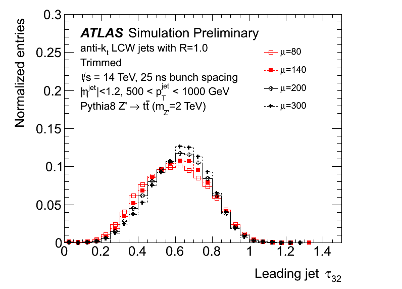 [pdf] [eps] |
| Distributions of N-subjettiness tau32 ratio [1] for the leading pT anti-kt trimmed R=1.0 jet in Z-> ttbar (mZ=2 TeV) (left) and dijet (right) events with mean number of interactions per bunch crossing (mu) of 80 (red closed squares),140 (red open squares), 200 (black open crosses) and 300 (black closed crosses). Jets with |eta|<1.2 and 0.5 TeV<pT<1 TeV are used. | 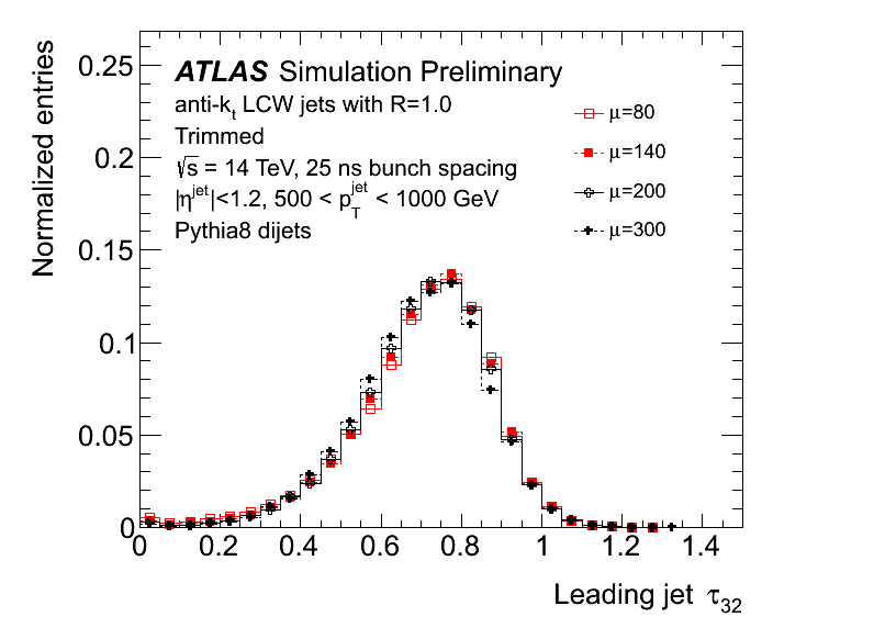 [pdf] [eps] |
| Top tagging performance under high luminosity conditions using a sqrt(d12) (left) and sqrt(d23) (right) scan. The y axis is one minus the efficiency to select background dijet events (fake rate) and the x-axis is the efficiency to select signal top jets. Jets with |eta|<1.2 and 0.5 TeV<pT<1 TeV are used. Each colored curve corresponds to different pileup conditions from mu=80 to mu=300. While the top tagging performance degrades with higher pileup, top tagging continues to work up to mu=300. No systematic uncertainties are included in these figures and there are several differences in settings such that small differences are not significant. | 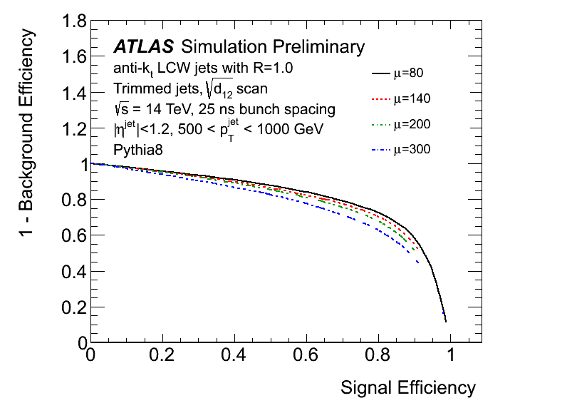 [pdf] [eps] |
| Top tagging performance under high luminosity conditions using a sqrt(d12) (left) and sqrt(d23) (right) scan. The y axis is one minus the efficiency to select background dijet events (fake rate) and the x-axis is the efficiency to select signal top jets. Jets with |eta|<1.2 and 0.5 TeV<pT<1 TeV are used. Each colored curve corresponds to different pileup conditions from mu=80 to mu=300. While the top tagging performance degrades with higher pileup, top tagging continues to work up to mu=300. No systematic uncertainties are included in these figures and there are several differences in settings such that small differences are not significant. |  [pdf] [eps] |
| Top tagging performance under high luminosity conditions using a tau32 scan. The y axis is one minus the efficiency to select background dijet events (fake rate) and the x-axis is the efficiency to select signal top jets. Jets with |eta|<1.2 and 0.5 TeV<pT<1 TeV are used. Each colored curve corresponds to different pileup conditions from mu=80 to mu=300. While the top tagging performance degrades with higher pileup, top tagging continues to work up to mu=300. No systematic uncertainties are included in these figures and there are several differences in settings such that small differences are not significant. | 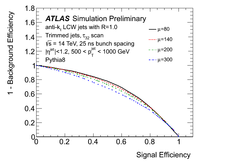 [pdf] [eps] |
| The anti-kt R=1.0 leading jet mass distribution before (left) and after (right) jet grooming and pileup subtraction in Z-> ttbar (mZ=2 TeV) events with mean number of interactions per bunch crossing (mu) of 0 (black closed circles), 80 (red closed squares),140 (red open squares), 200 (black open crosses) and 300 (black closed crosses). Jets with|eta|<1.2 and 0.5 TeV<pT<1 TeV are used. The left plot is for jets without any grooming or pileup subtraction and shows a significant effect of pileup on both the mean and width of the jet mass distribution and the top mass peak is not visible. In the right plot, jets are trimmed [5] with parameters fcut>5% and Rsubjet = 0.3 and are corrected for pileup using the Voronoi-area pileup subtraction [3]. With grooming and subtraction applied, the effect of pileup is highly reduced. The top mass peak and a smaller peak at the W mass are now visible. |  [pdf] [eps] |
| The anti-kt R=1.0 leading jet mass distribution before (left) and after (right) jet grooming and pileup subtraction in Z-> ttbar (mZ=2 TeV) events with mean number of interactions per bunch crossing (mu) of 0 (black closed circles), 80 (red closed squares),140 (red open squares), 200 (black open crosses) and 300 (black closed crosses). Jets with|eta|<1.2 and 0.5 TeV<pT<1 TeV are used. The left plot is for jets without any grooming or pileup subtraction and shows a significant effect of pileup on both the mean and width of the jet mass distribution and the top mass peak is not visible. In the right plot, jets are trimmed [5] with parameters fcut>5% and Rsubjet = 0.3 and are corrected for pileup using the Voronoi-area pileup subtraction [3]. With grooming and subtraction applied, the effect of pileup is highly reduced. The top mass peak and a smaller peak at the W mass are now visible. | 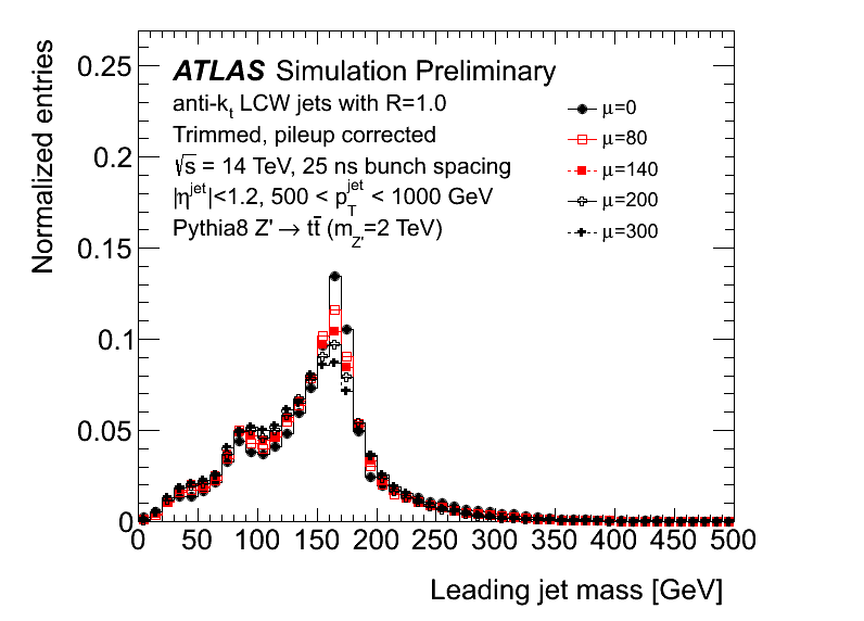 [pdf] [eps] |
| The anti-kt R=1.0 leading jet mass distribution before (left) and after (right) jet grooming and pileup subtraction in dijet events with mean number of interactions per bunch crossing (mu) of 0 (black closed circles), 80 (red closed squares),140 (red open squares), 200 (black open crosses) and 300 (black closed crosses). Jets with |eta|<1.2 and 0.5 TeV<pT<1 TeV are used. The left plot is for jets without any grooming or pileup subtraction. In the right plot, jets are trimmed [5] with parameters fcut>5% and Rsubjet = 0.3 and are corrected for pileup using the Voronoi-area pileup subtraction [3]. With grooming and subtraction applied, the effect of pileup is highly reduced and the mean mass is significantly shifted to smaller values. This isparticularly important to improve signal discrimination in analyses with high transverse momentum resonant signals. |  [pdf] [eps] |
| The anti-kt R=1.0 leading jet mass distribution before (left) and after (right) jet grooming and pileup subtraction in dijet events with mean number of interactions per bunch crossing (mu) of 0 (black closed circles), 80 (red closed squares),140 (red open squares), 200 (black open crosses) and 300 (black closed crosses). Jets with |eta|<1.2 and 0.5 TeV<pT<1 TeV are used. The left plot is for jets without any grooming or pileup subtraction. In the right plot, jets are trimmed [5] with parameters fcut>5% and Rsubjet = 0.3 and are corrected for pileup using the Voronoi-area pileup subtraction [3]. With grooming and subtraction applied, the effect of pileup is highly reduced and the mean mass is significantly shifted to smaller values. This isparticularly important to improve signal discrimination in analyses with high transverse momentum resonant signals. | 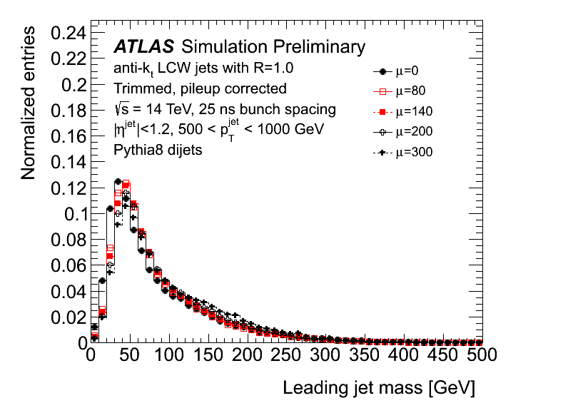 [pdf] [eps] |
References
- [1] Comput. Phys. Commun. 178 (2008) 852867
- [2] CERN-2012-022 , LHCC-I-023 (2012)
- [3] JHEP 0804 (2008) 005!
- [4] Nucl. Instrum. Meth. A 531 (2004) 481
- [5] arXiv:1306.4945
Major updates:
-- DavidLopezMateos - 18 Oct 2014 Responsible: DavidLopezMateos
Subject: public
Topic revision: r4 - 2014-10-20 - DavidLopezMateos

or Ideas, requests, problems regarding TWiki? use Discourse or Send feedback