

Compact Muon Solenoid
LHC, CERN
| CMS-PAS-B2G-16-020 | ||
| Search for new resonances decaying to $\mathrm{WW}/\mathrm{WZ} \to \ell\nu \mathrm{qq}$ | ||
| CMS Collaboration | ||
| August 2016 | ||
| Abstract: A search for massive narrow resonances decaying to pairs of W and Z bosons in the $\ell\nu\mathrm{qq}$ final state is presented, based on 12.9 fb$^{-1}$ of pp collision data collected in 2016 by the CMS experiment at the CERN LHC with a center-of-mass energy of 13 TeV. Spin-1 and spin-2 resonances corresponding to masses in the range 600-4500 GeV and decaying to WW/WZ are probed using the $\ell\nu\mathrm{qq}$ final state. Cross section and resonance mass exclusion limits are set for models that predict gravitons and heavy spin-1 bosons. | ||
| Links: CDS record (PDF) ; inSPIRE record ; CADI line (restricted) ; | ||
| Figures | |
png pdf |
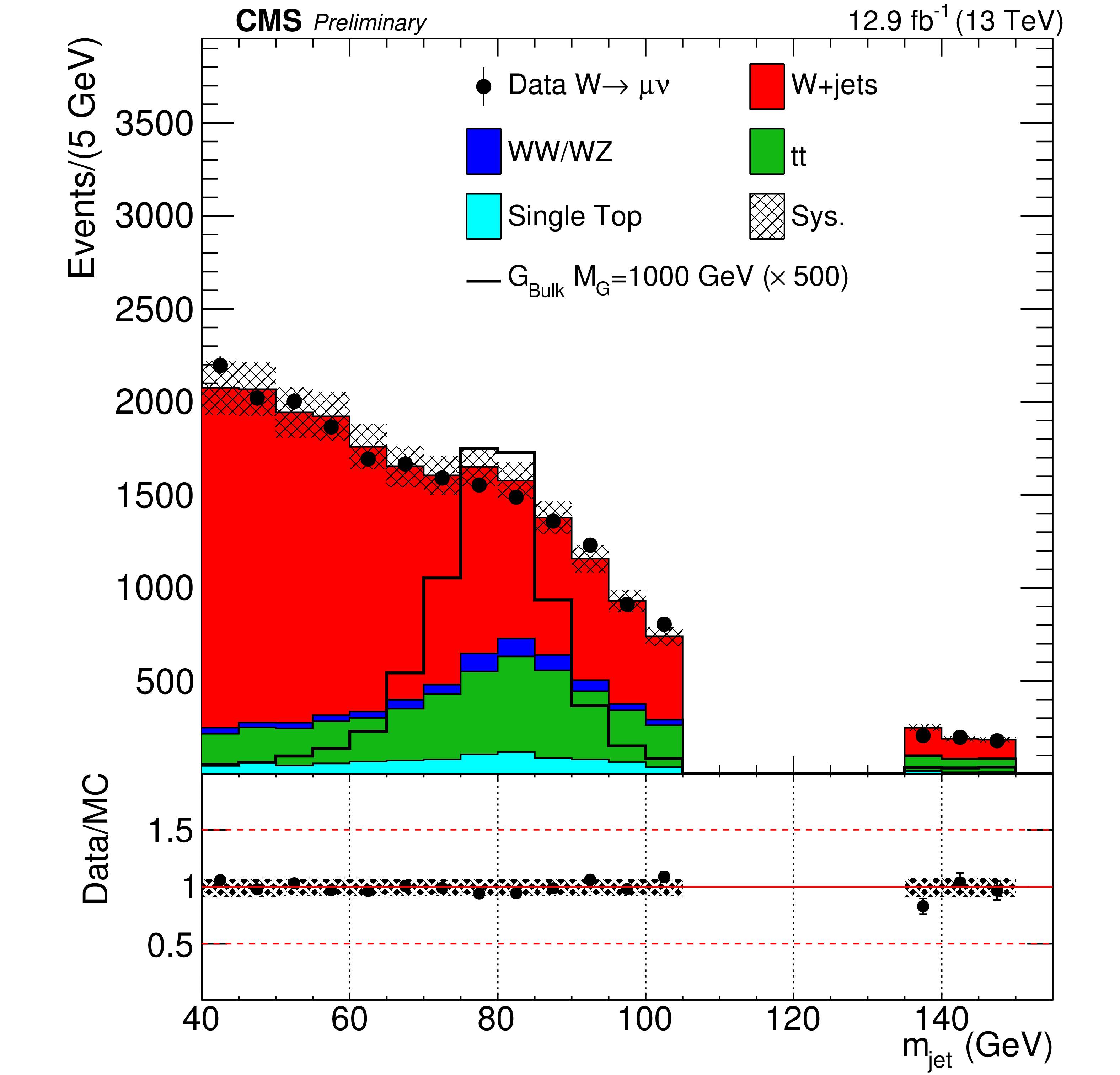
Figure 1-a:
Pruned jet mass and $N$-subjettiness ratio $\tau _{21}$ distributions in the ${m_{\text {jet}}}$ signal region and sideband. The signal distributions are scaled to an arbitrary cross section for better visualisation. The W+jets background from simulation is rescaled such that the total number of background events matches the number of events in data. The grey band represents the statistical uncertainty. a,b: muon channel; c,d: electron channel. |
png pdf |
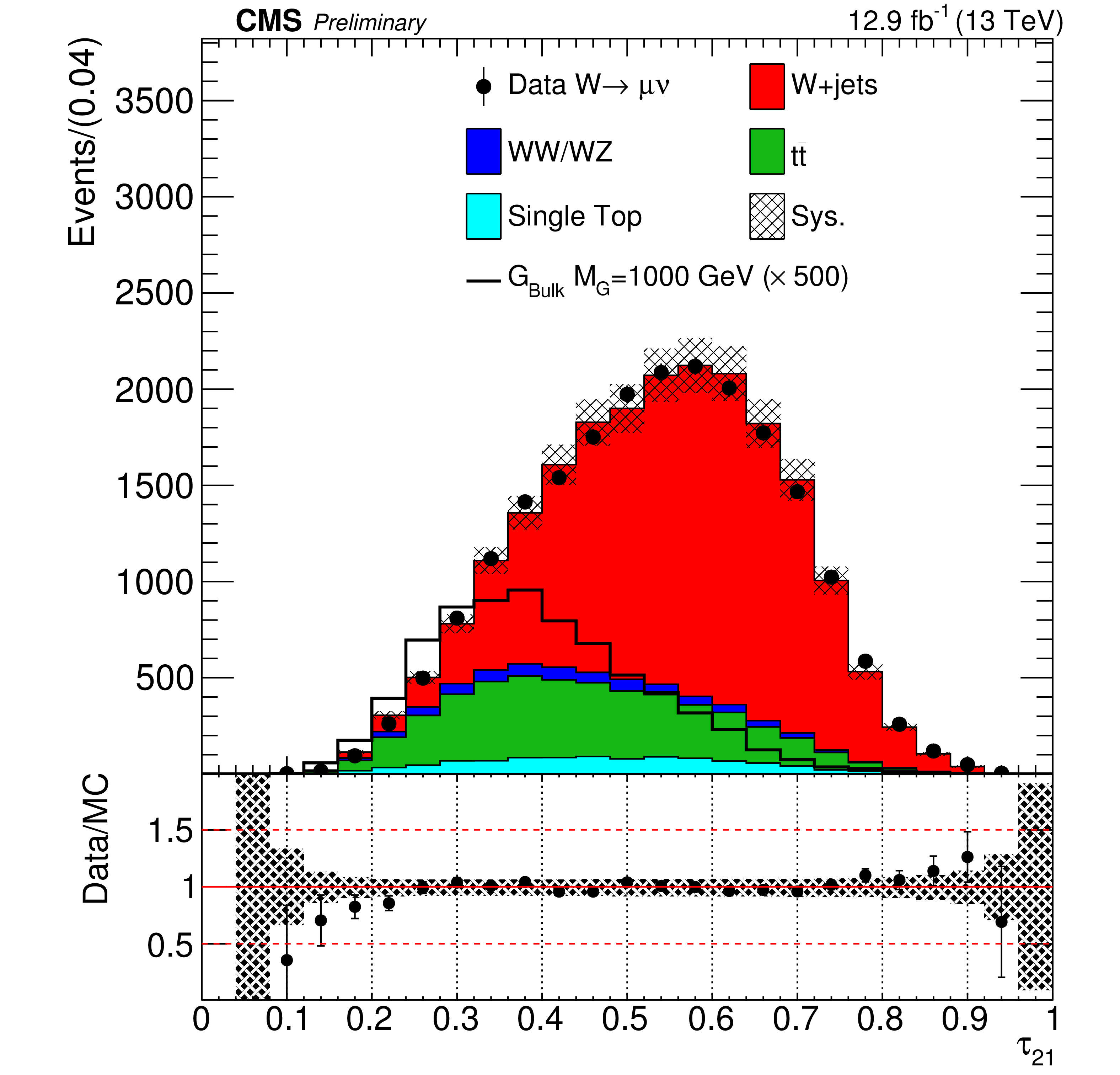
Figure 1-b:
Pruned jet mass and $N$-subjettiness ratio $\tau _{21}$ distributions in the ${m_{\text {jet}}}$ signal region and sideband. The signal distributions are scaled to an arbitrary cross section for better visualisation. The W+jets background from simulation is rescaled such that the total number of background events matches the number of events in data. The grey band represents the statistical uncertainty. a,b: muon channel; c,d: electron channel. |

png pdf |
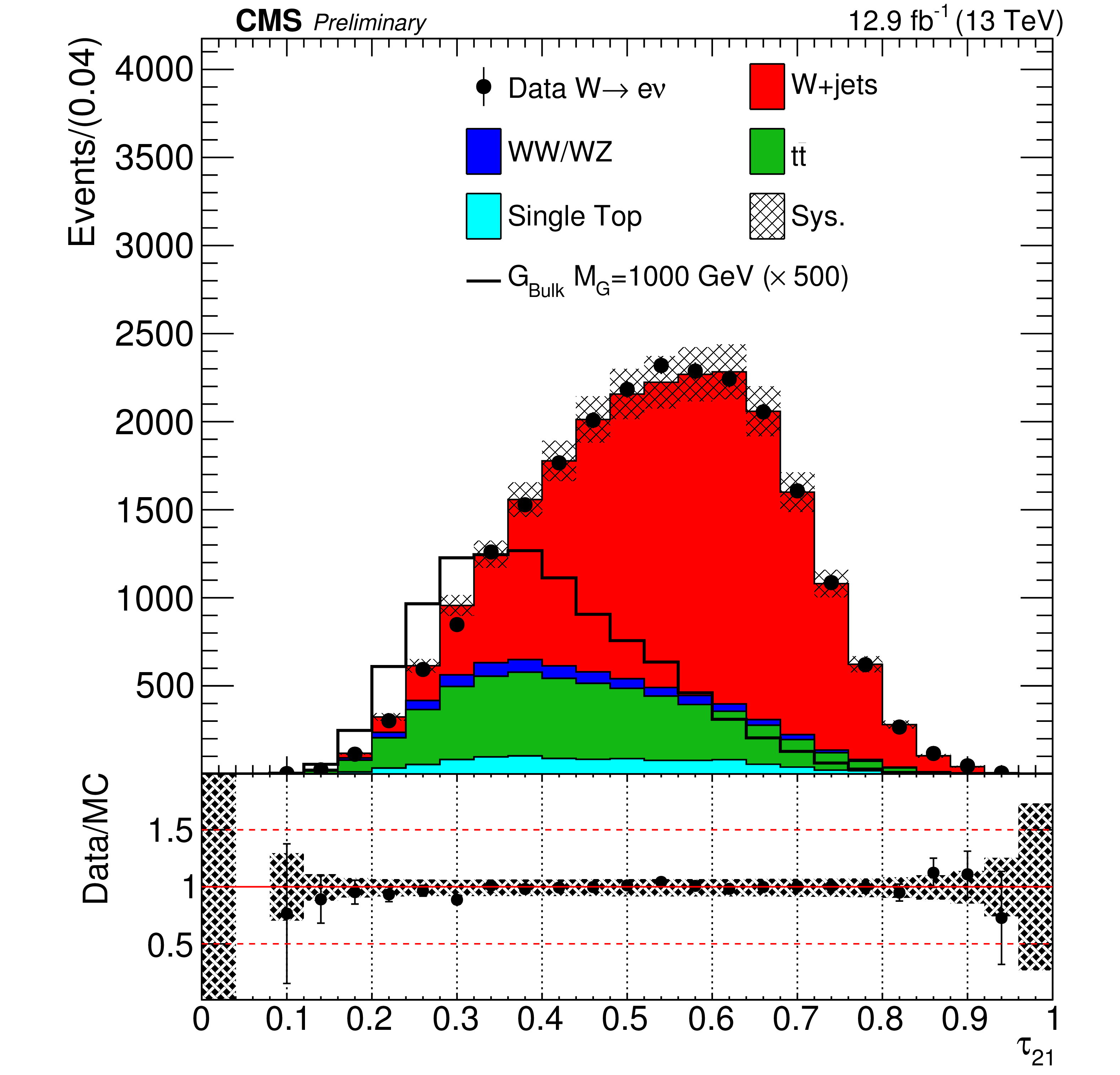
Figure 1-c:
Pruned jet mass and $N$-subjettiness ratio $\tau _{21}$ distributions in the ${m_{\text {jet}}}$ signal region and sideband. The signal distributions are scaled to an arbitrary cross section for better visualisation. The W+jets background from simulation is rescaled such that the total number of background events matches the number of events in data. The grey band represents the statistical uncertainty. a,b: muon channel; c,d: electron channel. |
png pdf |
Figure 1-d:
Pruned jet mass and $N$-subjettiness ratio $\tau _{21}$ distributions in the ${m_{\text {jet}}}$ signal region and sideband. The signal distributions are scaled to an arbitrary cross section for better visualisation. The W+jets background from simulation is rescaled such that the total number of background events matches the number of events in data. The grey band represents the statistical uncertainty. a,b: muon channel; c,d: electron channel. |
png pdf |
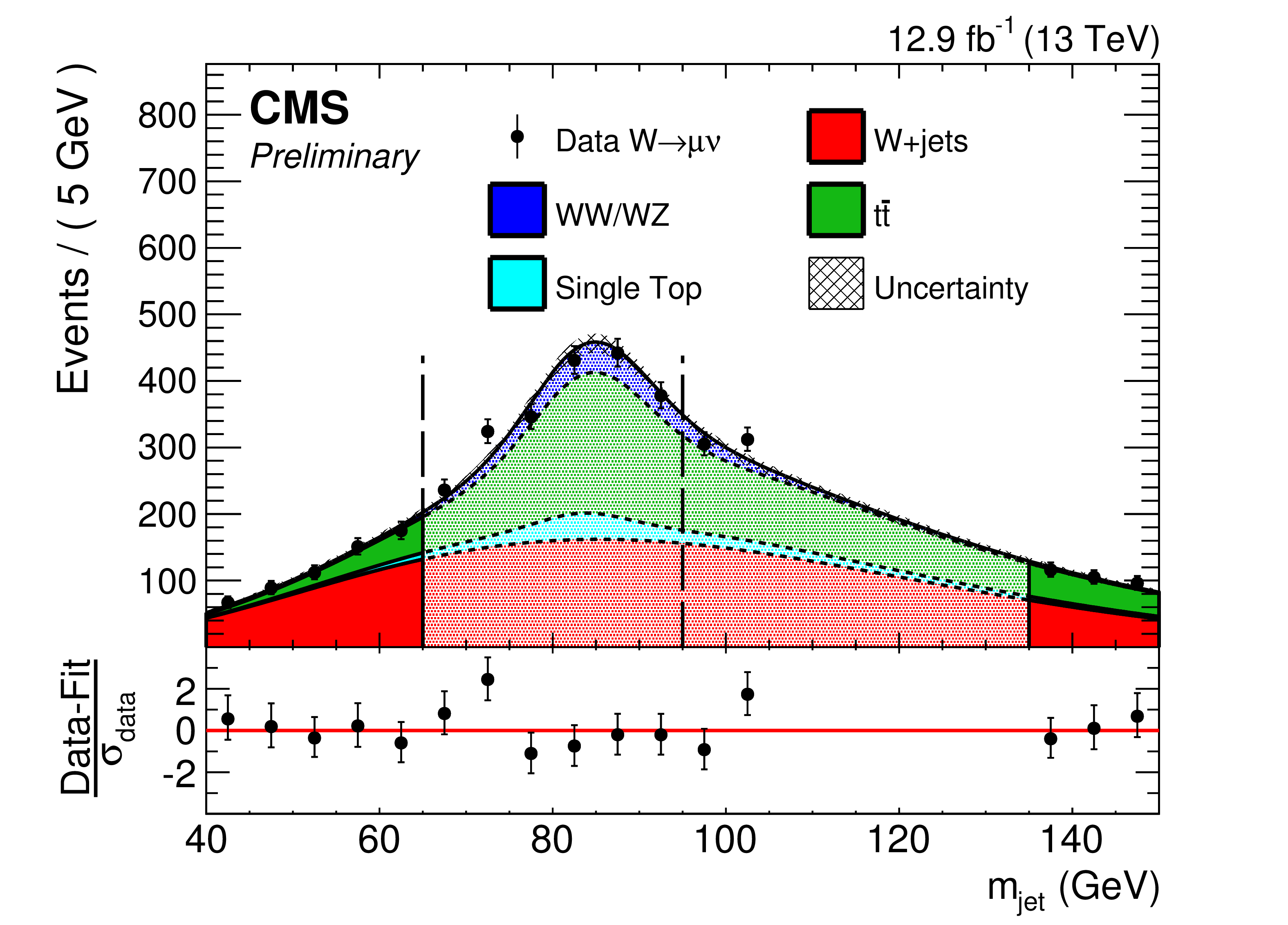
Figure 2-a:
Distributions of the pruned jet mass ${m_{\text {jet}}}$ in the muon (a,c) and electron (b,d) channels, for low mass (a,b) and high mass (c,d) region. The uncertainty band represents the statistical uncertainty on the background prediction. All selections are applied except the final ${m_{\text {jet}}}$ signal window requirement. Data are shown as black markers. The contribution of the W+jets background is extrapolated from the sideband to the signal region 65-95 GeV, which is represented with a grey shaded area and marked with a label. The grey shaded area between 95-135 GeV is not used in the analysis in order to avoid bias in future searches for WH, ZH and HH resonances. |

png pdf |
Figure 2-b:
Distributions of the pruned jet mass ${m_{\text {jet}}}$ in the muon (a,c) and electron (b,d) channels, for low mass (a,b) and high mass (c,d) region. The uncertainty band represents the statistical uncertainty on the background prediction. All selections are applied except the final ${m_{\text {jet}}}$ signal window requirement. Data are shown as black markers. The contribution of the W+jets background is extrapolated from the sideband to the signal region 65-95 GeV, which is represented with a grey shaded area and marked with a label. The grey shaded area between 95-135 GeV is not used in the analysis in order to avoid bias in future searches for WH, ZH and HH resonances. |

png pdf |
Figure 2-c:
Distributions of the pruned jet mass ${m_{\text {jet}}}$ in the muon (a,c) and electron (b,d) channels, for low mass (a,b) and high mass (c,d) region. The uncertainty band represents the statistical uncertainty on the background prediction. All selections are applied except the final ${m_{\text {jet}}}$ signal window requirement. Data are shown as black markers. The contribution of the W+jets background is extrapolated from the sideband to the signal region 65-95 GeV, which is represented with a grey shaded area and marked with a label. The grey shaded area between 95-135 GeV is not used in the analysis in order to avoid bias in future searches for WH, ZH and HH resonances. |

png pdf |
Figure 2-d:
Distributions of the pruned jet mass ${m_{\text {jet}}}$ in the muon (a,c) and electron (b,d) channels, for low mass (a,b) and high mass (c,d) region. The uncertainty band represents the statistical uncertainty on the background prediction. All selections are applied except the final ${m_{\text {jet}}}$ signal window requirement. Data are shown as black markers. The contribution of the W+jets background is extrapolated from the sideband to the signal region 65-95 GeV, which is represented with a grey shaded area and marked with a label. The grey shaded area between 95-135 GeV is not used in the analysis in order to avoid bias in future searches for WH, ZH and HH resonances. |

png pdf |
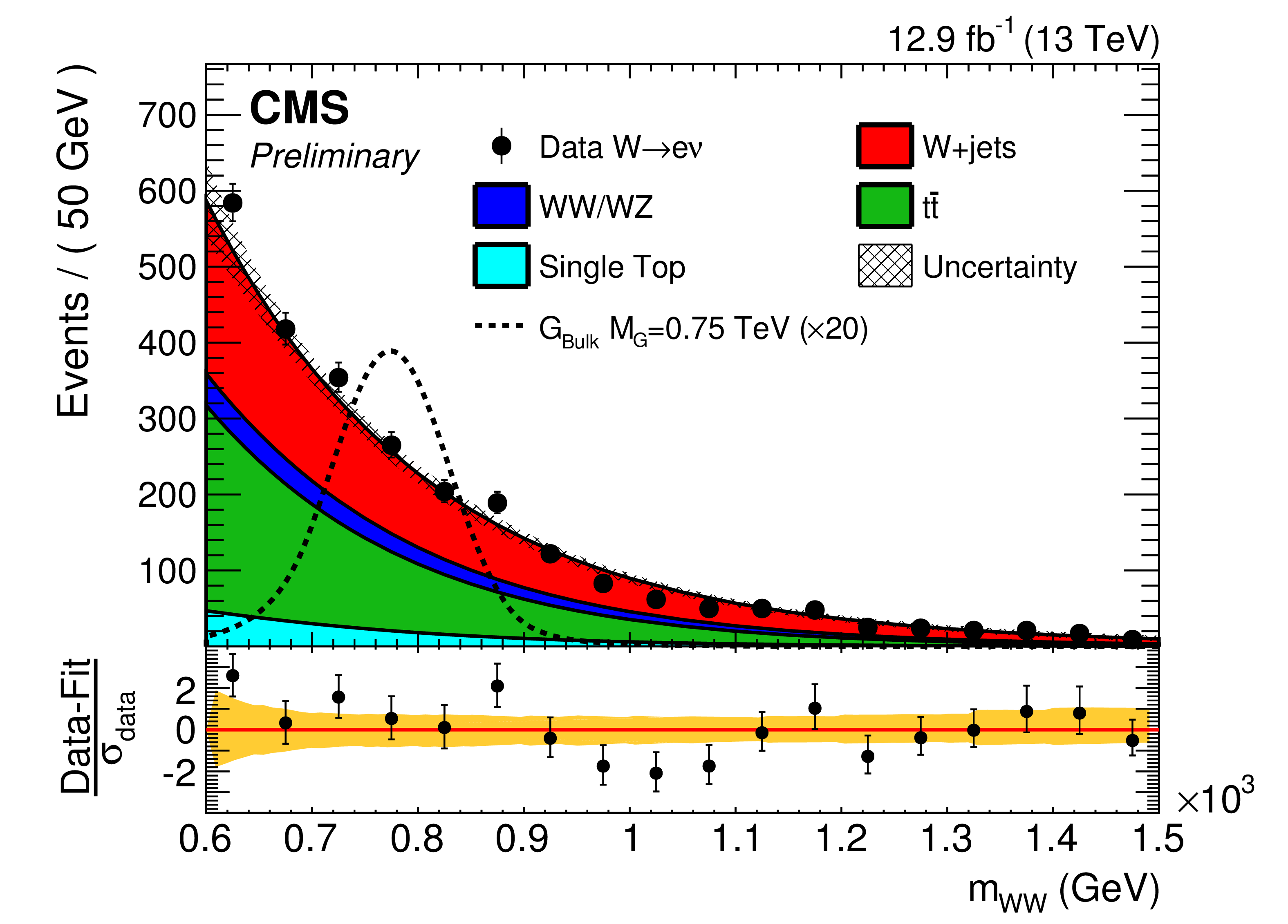
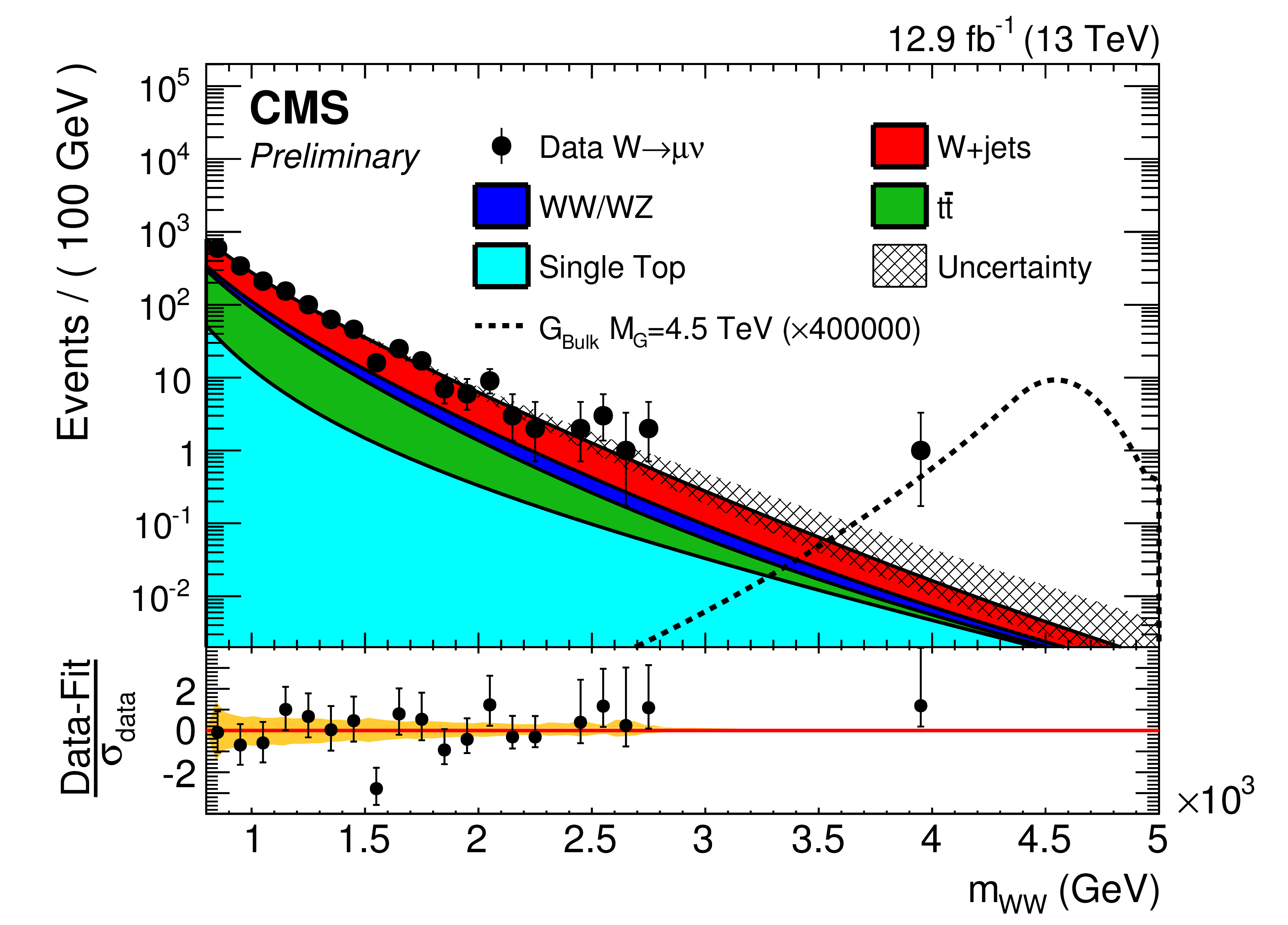
Figure 3-a:
Final observed $ {m_{ {\mathrm {W}} {\mathrm {W}} }} $ distributions for the WW analyses in the signal region. (a,c) and (b,d) plots show muon and electron channels. (a,b) and (c,d) plots show low and high mass. The solid curve represents the background estimation provided by the data-driven method as discussed in Sec. 6.1. The hatched band includes both statistical and systematic (of normalization and of shape) uncertainties. The data are shown as black markers. The bottom panels show the corresponding pull distributions, quantifying the agreement between the background-only hypothesis and the data. The pull distribution is defined as the difference between the data and the background prediction, divided by the error on data. The error bars on the points represent the statistical uncertainty of the data, while the uncertainty band (statistics+systematics) on the background prediction is shown with a yellow band. |
png pdf |
Figure 3-b:
Final observed $ {m_{ {\mathrm {W}} {\mathrm {W}} }} $ distributions for the WW analyses in the signal region. (a,c) and (b,d) plots show muon and electron channels. (a,b) and (c,d) plots show low and high mass. The solid curve represents the background estimation provided by the data-driven method as discussed in Sec. 6.1. The hatched band includes both statistical and systematic (of normalization and of shape) uncertainties. The data are shown as black markers. The bottom panels show the corresponding pull distributions, quantifying the agreement between the background-only hypothesis and the data. The pull distribution is defined as the difference between the data and the background prediction, divided by the error on data. The error bars on the points represent the statistical uncertainty of the data, while the uncertainty band (statistics+systematics) on the background prediction is shown with a yellow band. |
png pdf |
Figure 3-c:
Final observed $ {m_{ {\mathrm {W}} {\mathrm {W}} }} $ distributions for the WW analyses in the signal region. (a,c) and (b,d) plots show muon and electron channels. (a,b) and (c,d) plots show low and high mass. The solid curve represents the background estimation provided by the data-driven method as discussed in Sec. 6.1. The hatched band includes both statistical and systematic (of normalization and of shape) uncertainties. The data are shown as black markers. The bottom panels show the corresponding pull distributions, quantifying the agreement between the background-only hypothesis and the data. The pull distribution is defined as the difference between the data and the background prediction, divided by the error on data. The error bars on the points represent the statistical uncertainty of the data, while the uncertainty band (statistics+systematics) on the background prediction is shown with a yellow band. |

png pdf |
Figure 3-d:
Final observed $ {m_{ {\mathrm {W}} {\mathrm {W}} }} $ distributions for the WW analyses in the signal region. (a,c) and (b,d) plots show muon and electron channels. (a,b) and (c,d) plots show low and high mass. The solid curve represents the background estimation provided by the data-driven method as discussed in Sec. 6.1. The hatched band includes both statistical and systematic (of normalization and of shape) uncertainties. The data are shown as black markers. The bottom panels show the corresponding pull distributions, quantifying the agreement between the background-only hypothesis and the data. The pull distribution is defined as the difference between the data and the background prediction, divided by the error on data. The error bars on the points represent the statistical uncertainty of the data, while the uncertainty band (statistics+systematics) on the background prediction is shown with a yellow band. |

png pdf |
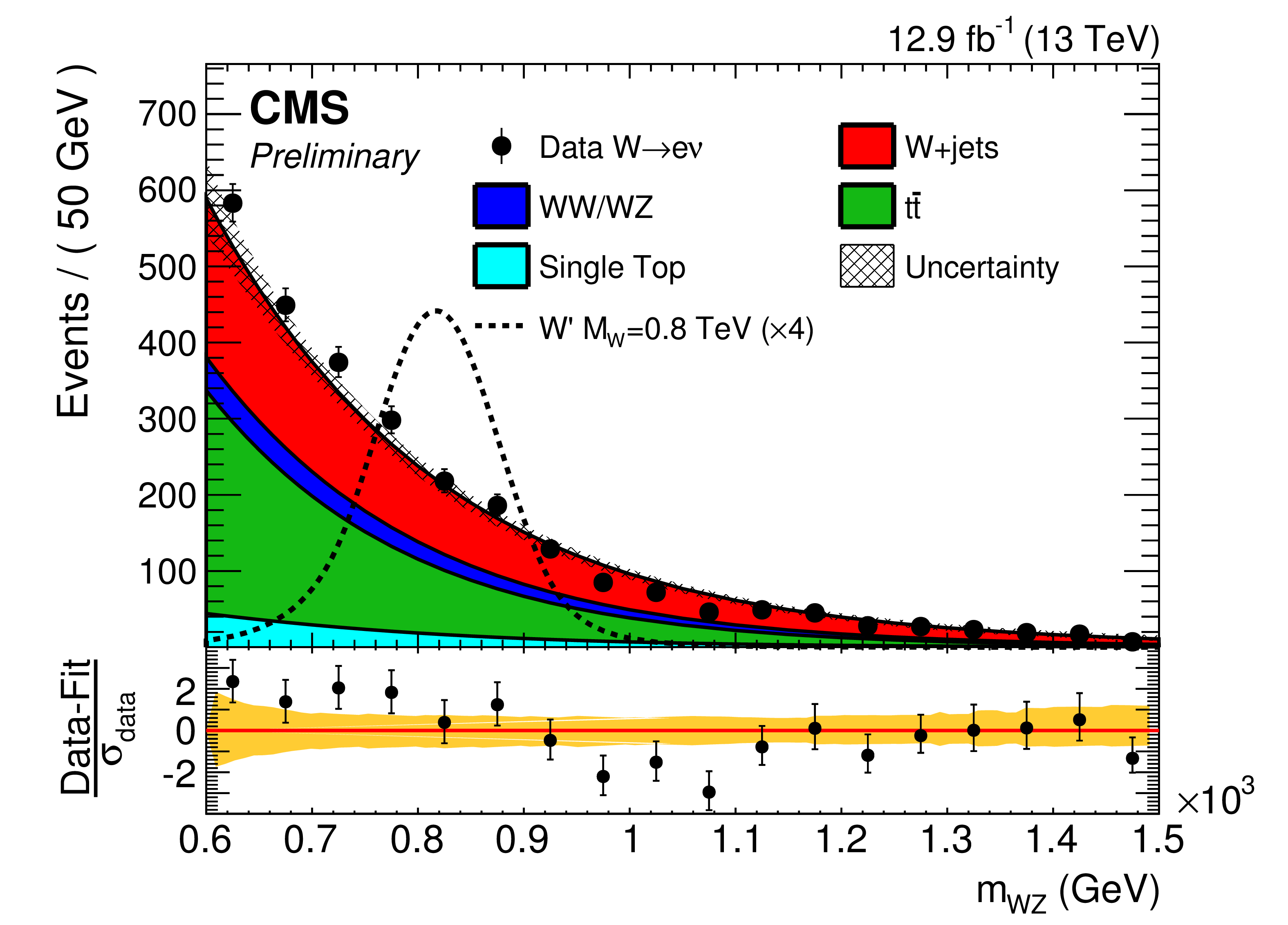
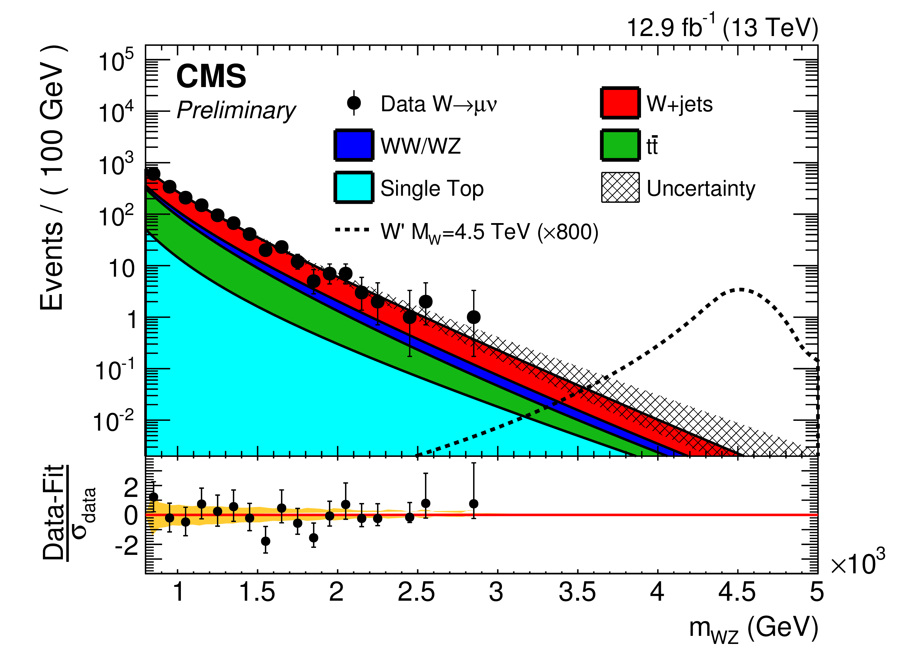
Figure 4-a:
Final observed $ {m_{ {\mathrm {W}} {\mathrm {Z}} }} $ distributions for the WZ analyses in the signal region. (a,c) and (b,d) plots show muon and electron channels. (a,b) and (c,d) plots show low and high mass. The solid curve represents the background estimation provided by the data-driven method as discussed in Sec. 6.1. The hatched band includes both statistical and systematic (of normalization and of shape) uncertainties. The data are shown as black markers. The bottom panels show the corresponding pull distributions, quantifying the agreement between the background-only hypothesis and the data. The pull distribution is defined as the difference between the data and the background prediction, divided by the error on data. The error bars on the points represent the statistical uncertainty of the data, while the uncertainty band (statistics+systematics) on the background prediction is shown with a yellow band. |
png pdf |
Figure 4-b:
Final observed $ {m_{ {\mathrm {W}} {\mathrm {Z}} }} $ distributions for the WZ analyses in the signal region. (a,c) and (b,d) plots show muon and electron channels. (a,b) and (c,d) plots show low and high mass. The solid curve represents the background estimation provided by the data-driven method as discussed in Sec. 6.1. The hatched band includes both statistical and systematic (of normalization and of shape) uncertainties. The data are shown as black markers. The bottom panels show the corresponding pull distributions, quantifying the agreement between the background-only hypothesis and the data. The pull distribution is defined as the difference between the data and the background prediction, divided by the error on data. The error bars on the points represent the statistical uncertainty of the data, while the uncertainty band (statistics+systematics) on the background prediction is shown with a yellow band. |
png pdf |
Figure 4-c:
Final observed $ {m_{ {\mathrm {W}} {\mathrm {Z}} }} $ distributions for the WZ analyses in the signal region. (a,c) and (b,d) plots show muon and electron channels. (a,b) and (c,d) plots show low and high mass. The solid curve represents the background estimation provided by the data-driven method as discussed in Sec. 6.1. The hatched band includes both statistical and systematic (of normalization and of shape) uncertainties. The data are shown as black markers. The bottom panels show the corresponding pull distributions, quantifying the agreement between the background-only hypothesis and the data. The pull distribution is defined as the difference between the data and the background prediction, divided by the error on data. The error bars on the points represent the statistical uncertainty of the data, while the uncertainty band (statistics+systematics) on the background prediction is shown with a yellow band. |
png pdf |
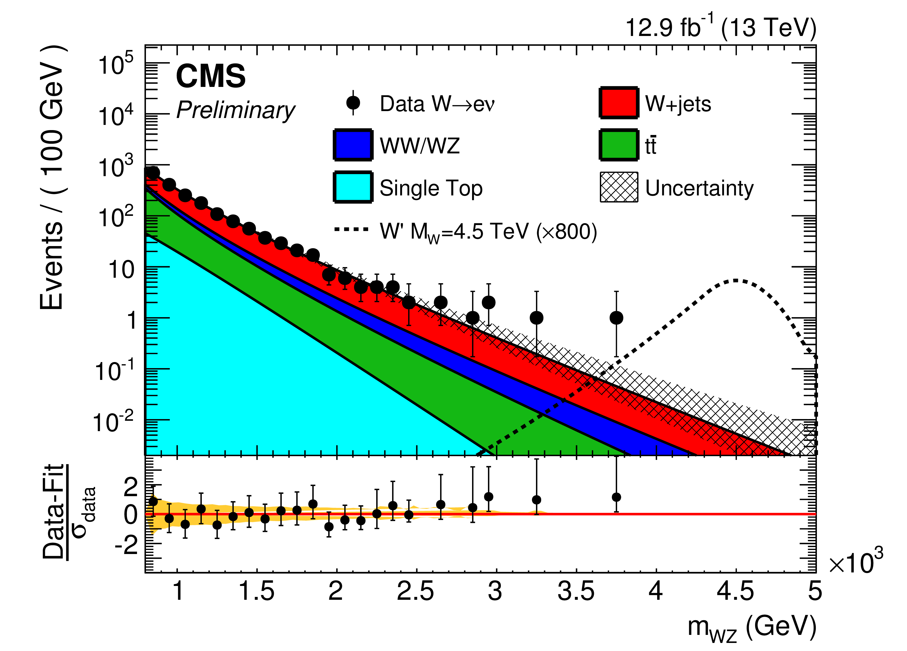
Figure 4-d:
Final observed $ {m_{ {\mathrm {W}} {\mathrm {Z}} }} $ distributions for the WZ analyses in the signal region. (a,c) and (b,d) plots show muon and electron channels. (a,b) and (c,d) plots show low and high mass. The solid curve represents the background estimation provided by the data-driven method as discussed in Sec. 6.1. The hatched band includes both statistical and systematic (of normalization and of shape) uncertainties. The data are shown as black markers. The bottom panels show the corresponding pull distributions, quantifying the agreement between the background-only hypothesis and the data. The pull distribution is defined as the difference between the data and the background prediction, divided by the error on data. The error bars on the points represent the statistical uncertainty of the data, while the uncertainty band (statistics+systematics) on the background prediction is shown with a yellow band. |
png pdf |
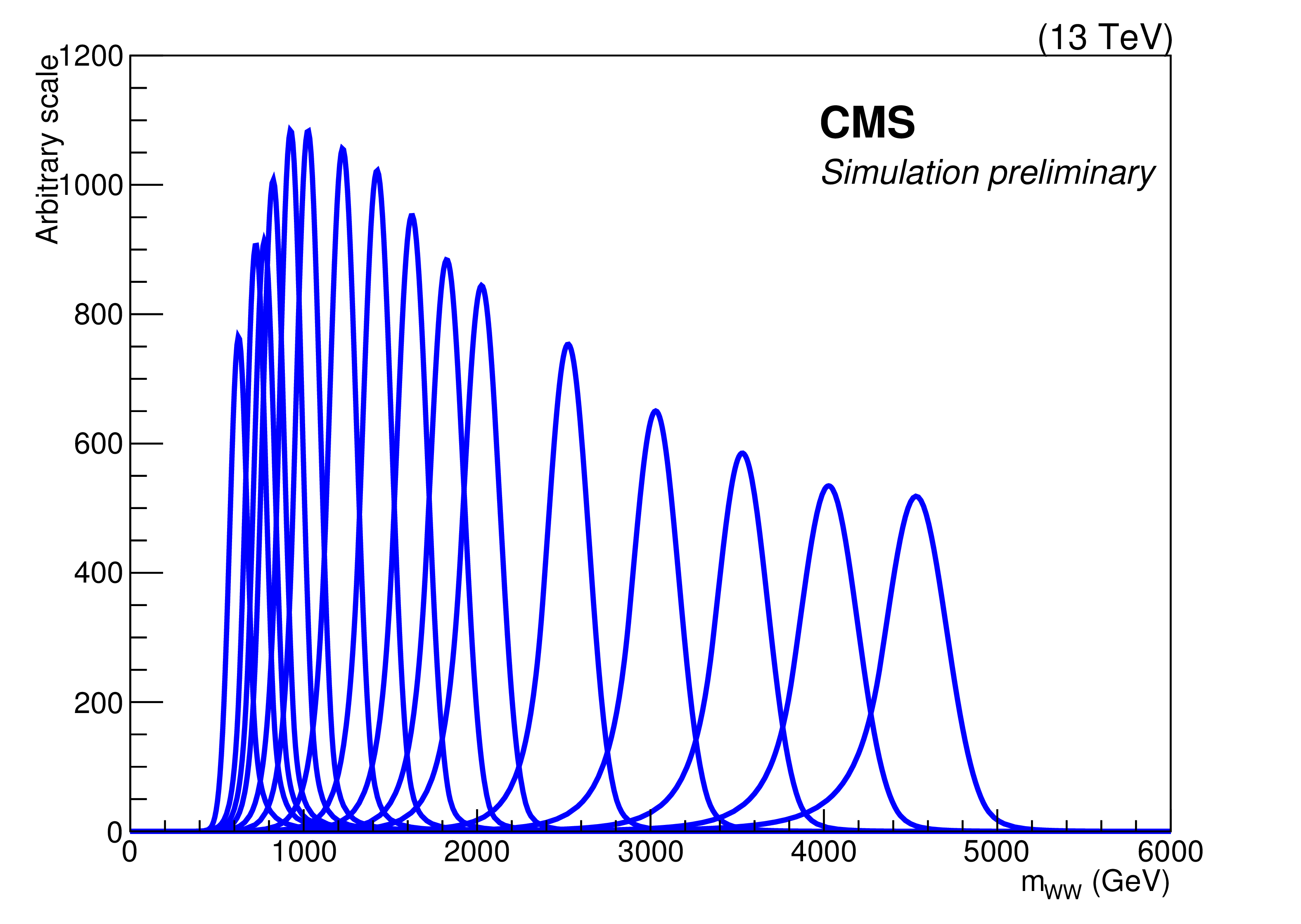
Figure 5:
$m_{\mathrm {WW}}$ distribution for different signal mass points. The area of each shape is proportional to the total signal efficiency of the corresponding mass point. |
png pdf |
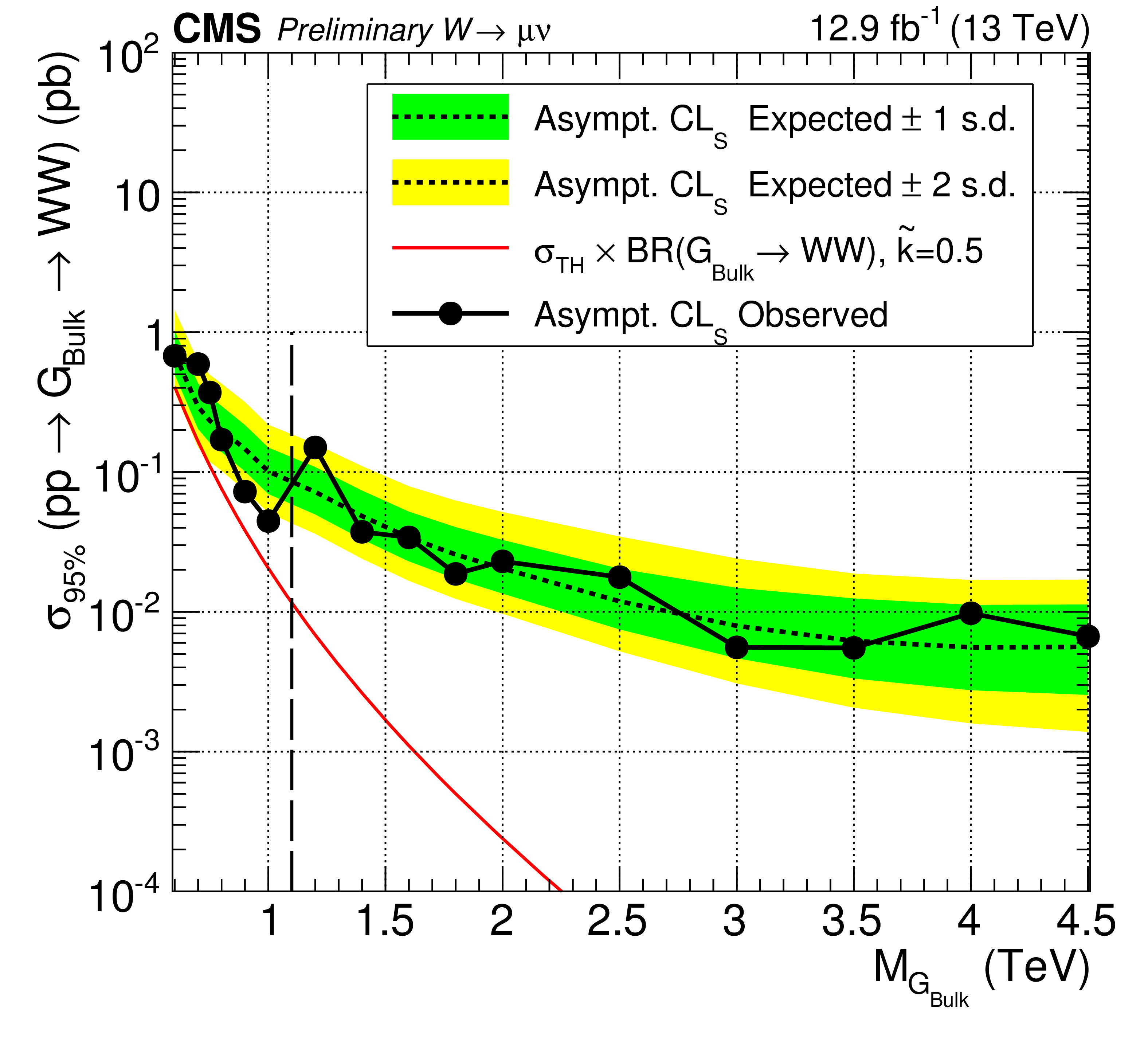
Figure 6-a:
Observed (black solid) and expected (black dashed) 95% CL upper limits on the product of the graviton production cross section and the branching fraction of $ { {\mathrm {G}} _{\mathrm {bulk}}}\to {\mathrm {W}} {\mathrm {W}}$ in the muon (a) and electron (b) channel. The theoretical cross section multiplied by the relevant branching ratio is shown as a red solid line. The dashed vertical line delineates the transition between the low and high mass searches. |
png pdf |
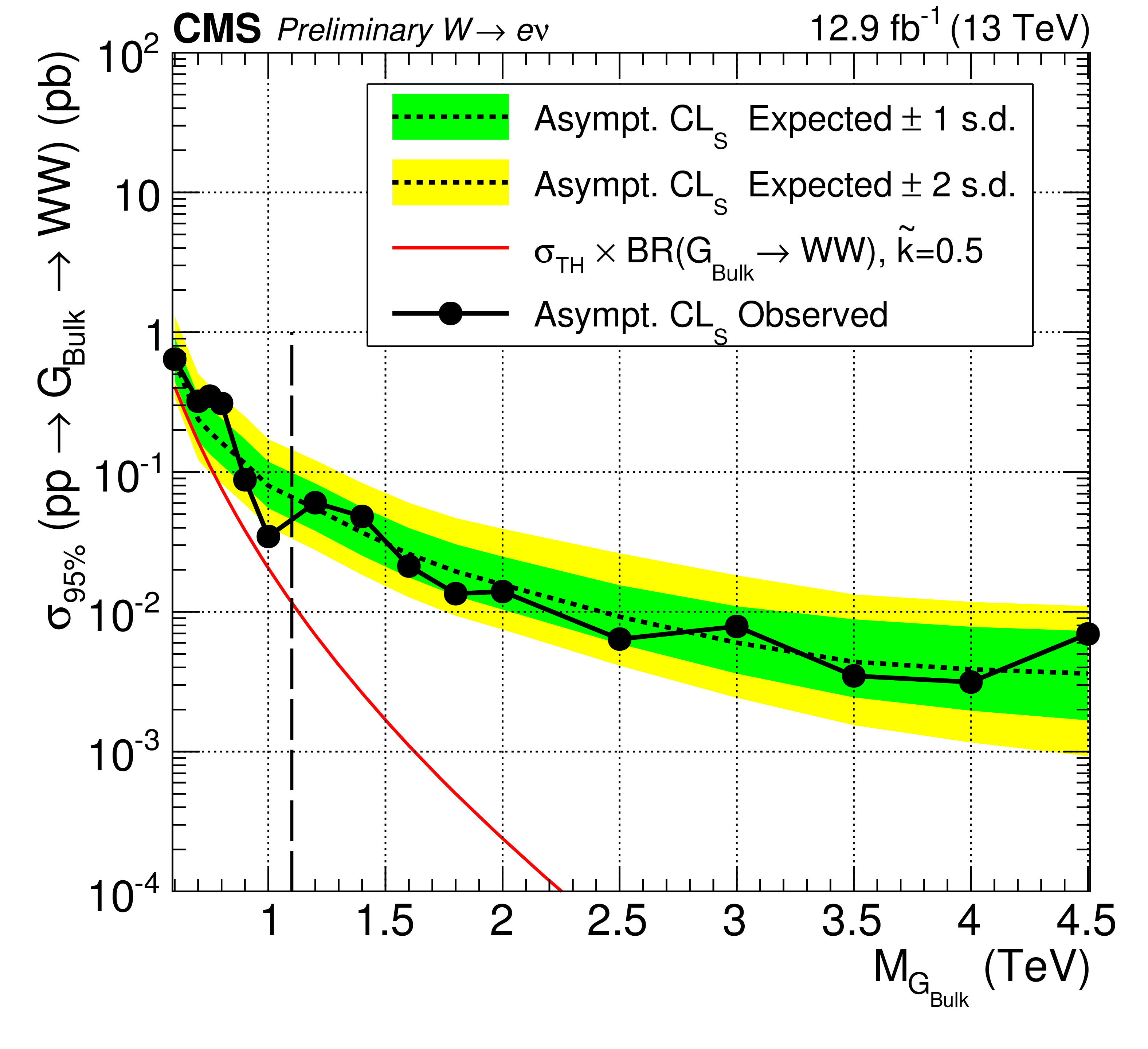
Figure 6-b:
Observed (black solid) and expected (black dashed) 95% CL upper limits on the product of the graviton production cross section and the branching fraction of $ { {\mathrm {G}} _{\mathrm {bulk}}}\to {\mathrm {W}} {\mathrm {W}}$ in the muon (a) and electron (b) channel. The theoretical cross section multiplied by the relevant branching ratio is shown as a red solid line. The dashed vertical line delineates the transition between the low and high mass searches. |

png pdf |
Figure 7:
Observed (black solid) and expected (black dashed) 95% CL upper limits on the product of the graviton production cross section and the branching fraction of $ { {\mathrm {G}} _{\mathrm {bulk}}}\to {\mathrm {W}} {\mathrm {W}}$ for the statistical combination of electron and muon channels. The theoretical cross section multiplied by the relevant branching ratio is shown as a red solid line. The dashed vertical line delineates the transition between the low and high mass searches. |

png pdf |
Figure 8-a:
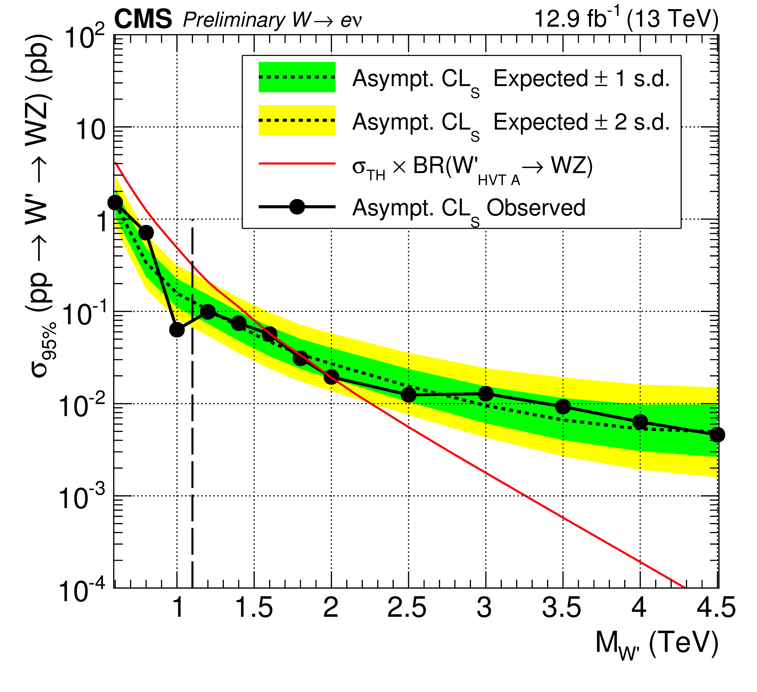
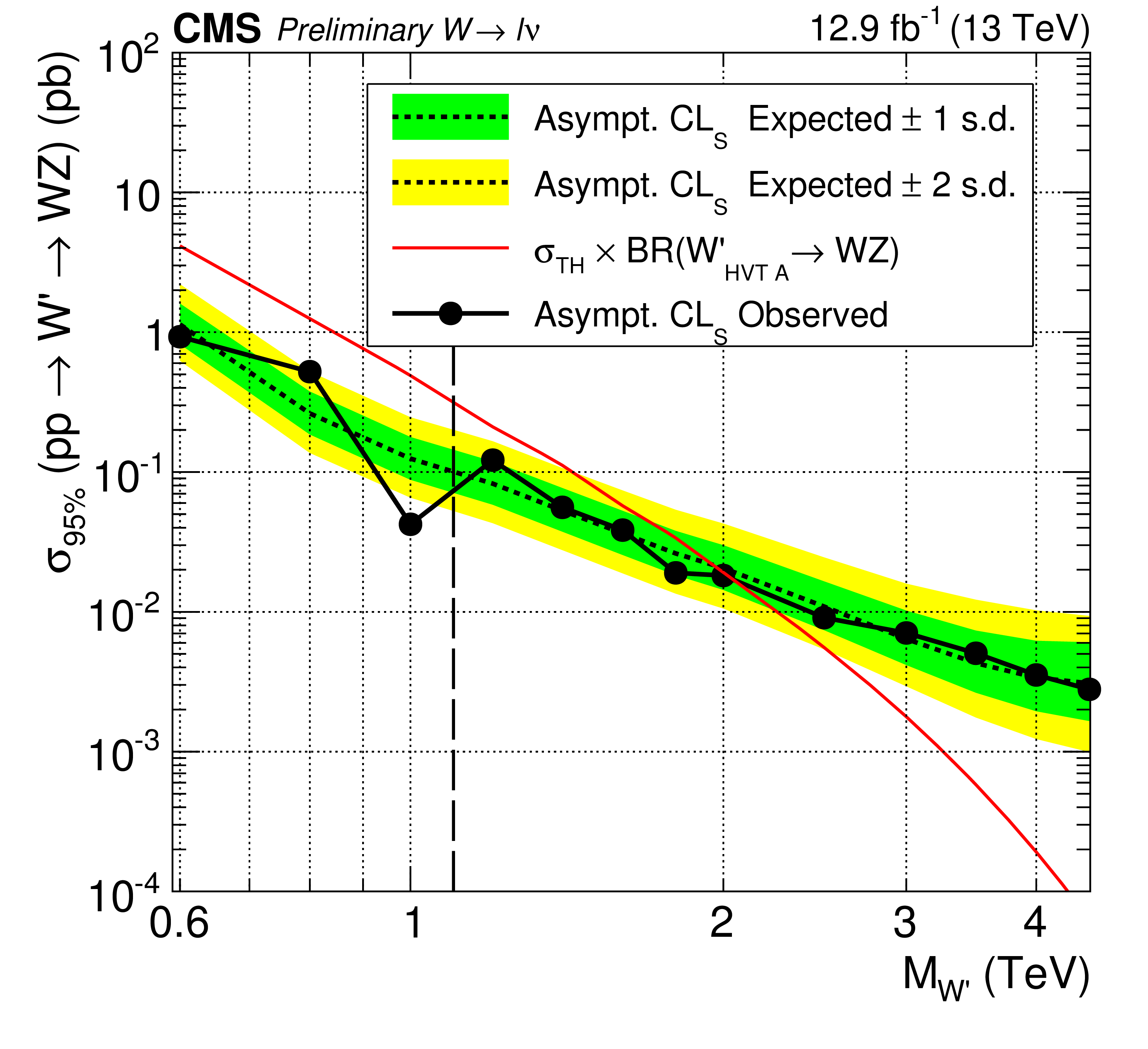
Observed (black solid) and expected (black dashed) 95% CL upper limits on the product of the W' production cross section and the branching fraction of $\mathrm{ W' } \to {\mathrm {W}} {\mathrm {Z}} $ in the muon (a) and electron (b) channel. The theoretical cross section multiplied by the relevant branching ratio is shown as a red solid line. The dashed vertical line delineates the transition between the low and high mass searches. |
png pdf |
Figure 8-b:
Observed (black solid) and expected (black dashed) 95% CL upper limits on the product of the W' production cross section and the branching fraction of $\mathrm{ W' } \to {\mathrm {W}} {\mathrm {Z}} $ in the muon (a) and electron (b) channel. The theoretical cross section multiplied by the relevant branching ratio is shown as a red solid line. The dashed vertical line delineates the transition between the low and high mass searches. |
png pdf |
Figure 9:
Observed (black solid) and expected (black dashed) 95% CL upper limits on the product of the W' production cross section and the branching fraction of $\mathrm{ W' } \to {\mathrm {W}} {\mathrm {Z}} $ for the statistical combination of electron and muon channels. The theoretical cross section multiplied by the relevant branching ratio is shown as a red solid line. The dashed vertical line delineates the transition between the low and high mass searches. |
| Tables | |
png pdf |
Table 1:
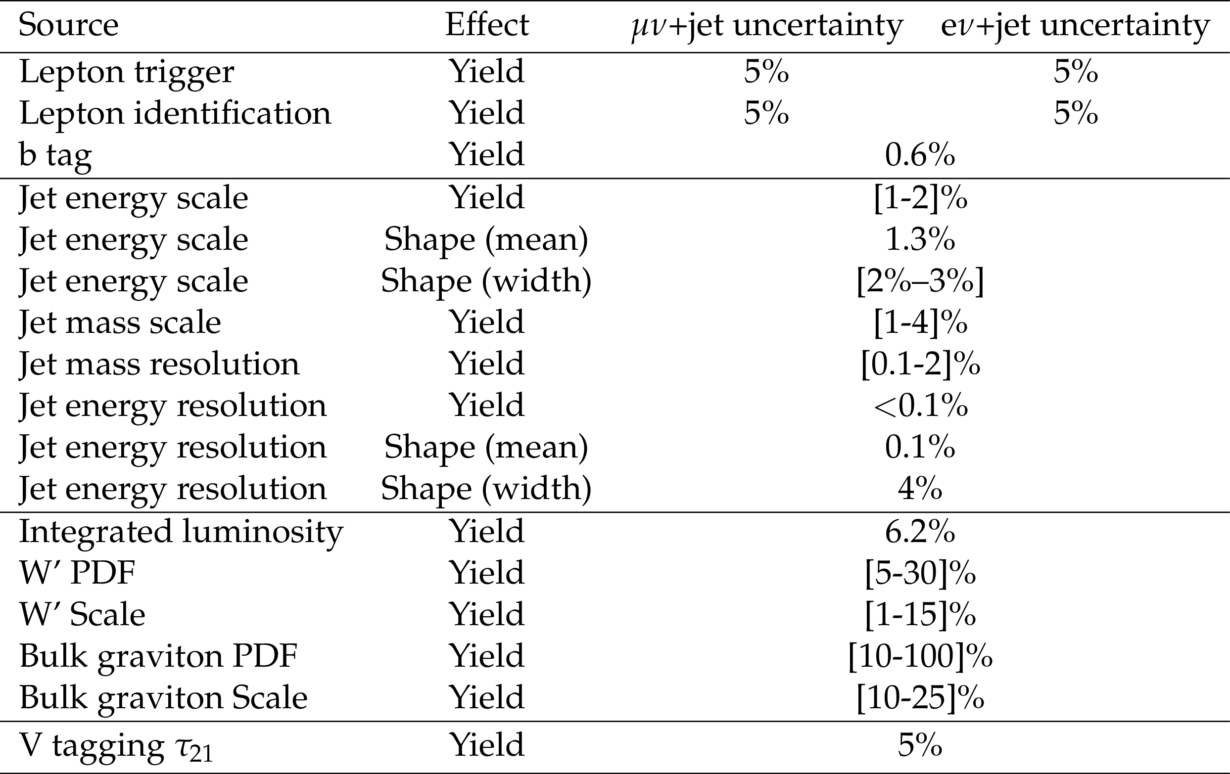
Summary of the systematic uncertainties and their impact on the signal yield and reconstructed ${m_{ {\mathrm {W}} {\mathrm {V}} }} $ shape (mean and width) for both muon and electron channels. Ranges are denoted in square brackets. |
png pdf |
Table 2:
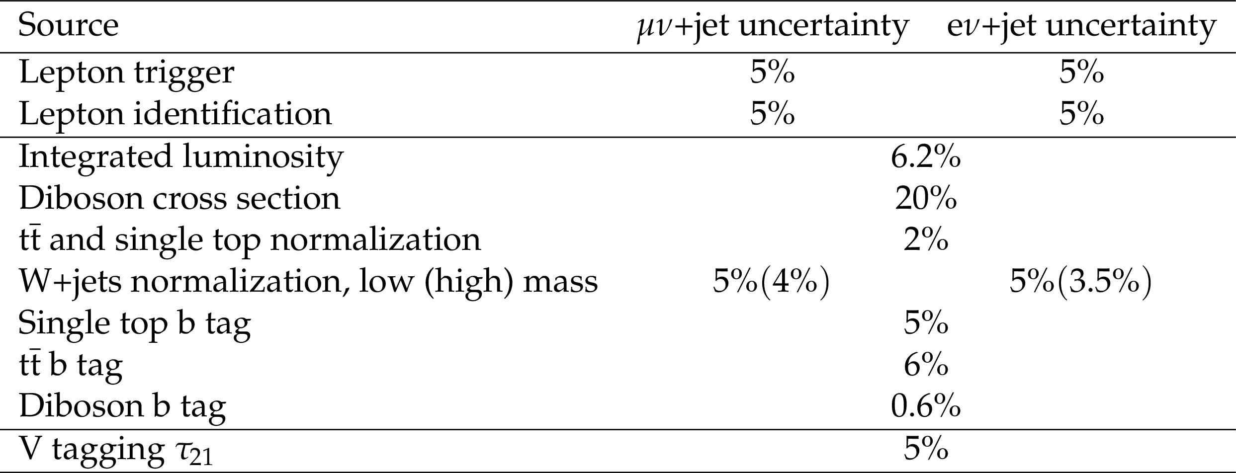
Systematic uncertainties affecting the background normalization. Ranges are denoted in square brackets. |
| Summary |
| We have presented a search for new resonances decaying to WW and WZ in which one of the bosons decays hadronically. The final state considered is $\ell \nu {\mathrm{ q q' }} $ with $\ell=\mu$ or e. The results include the case in which $\mathrm{ W } \to \tau\nu$ where $\tau$ decays leptonically. W or Z bosons that decay to quarks are identified by requiring a jet with mass compatible with the W or Z boson mass. Additional information from jet substructure is used to reduce the background from W+jets and multijet processes. No evidence for a signal is found, and upper limits at 95% CL are set for resonance masses between 600 and 4500 GeV on the bulk graviton $\rightarrow \mathrm{ WW } $ and HVT $ \mathrm{ W' } \rightarrow \mathrm{ W }\mathrm{ Z } $ production cross section, in the range of 400 to 4 fb and 1000 to 3 fb, respectively. These cross section limits are the most stringent to date in these final states. |
| References | ||||
| 1 | K. Agashe, H. Davoudiasl, G. Perez, and A. Soni | Warped Gravitons at the LHC and Beyond | PRD 76 (2007) 036006 | hep-ph/0701186 |
| 2 | A. L. Fitzpatrick, J. Kaplan, L. Randall, and L.-T. Wang | Searching for the Kaluza-Klein Graviton in Bulk RS Models | JHEP 09 (2007) 013 | hep-ph/0701150 |
| 3 | O. Antipin, D. Atwood, and A. Soni | Search for RS gravitons via W(L)W(L) decays | PLB 666 (2008) 155--161 | 0711.3175 |
| 4 | L. Randall and R. Sundrum | A Large mass hierarchy from a small extra dimension | PRL 83 (1999) 3370--3373 | hep-ph/9905221 |
| 5 | L. Randall and R. Sundrum | An Alternative to compactification | PRL 83 (1999) 4690--4693 | hep-th/9906064 |
| 6 | D. Pappadopulo, A. Thamm, R. Torre, and A. Wulzer | Heavy Vector Triplets: Bridging Theory and Data | JHEP 09 (2014) 060 | 1402.4431 |
| 7 | ATLAS Collaboration | Searches for heavy diboson resonances in $ pp $ collisions at $ \sqrt{s}=13 $ TeV with the ATLAS detector | 1606.04833 | |
| 8 | CMS Collaboration | Search for WW in semileptonic final states: low mass extension | CMS-PAS-B2G-16-004 | CMS-PAS-B2G-16-004 |
| 9 | CMS Collaboration | Combination of diboson resonance searches at 8 and 13 TeV | CMS-PAS-B2G-16-007 | CMS-PAS-B2G-16-007 |
| 10 | CMS Collaboration | Particle-Flow Event Reconstruction in CMS and Performance for Jets, Taus, and MET | CDS | |
| 11 | CMS Collaboration | Commissioning of the Particle-flow Event Reconstruction with the first LHC collisions recorded in the CMS detector | CDS | |
| 12 | CMS Collaboration | The CMS experiment at the CERN LHC | JINST 3 (2008) S08004 | CMS-00-001 |
| 13 | J. Alwall et al. | The automated computation of tree-level and next-to-leading order differential cross sections, and their matching to parton shower simulations | JHEP 07 (2014) 079 | 1405.0301 |
| 14 | P. Nason | A New method for combining NLO QCD with shower Monte Carlo algorithms | JHEP 11 (2004) 040 | hep-ph/0409146 |
| 15 | S. Frixione, P. Nason, and C. Oleari | Matching NLO QCD computations with Parton Shower simulations: the POWHEG method | JHEP 11 (2007) 070 | 0709.2092 |
| 16 | S. Alioli, P. Nason, C. Oleari, and E. Re | A general framework for implementing NLO calculations in shower Monte Carlo programs: the POWHEG BOX | JHEP 06 (2010) 043 | 1002.2581 |
| 17 | S. Alioli, P. Nason, C. Oleari, and E. Re | NLO single-top production matched with shower in POWHEG: s- and t-channel contributions | JHEP 09 (2009) 111, , [Erratum: JHEP02,011(2010)] | 0907.4076 |
| 18 | E. Re | Single-top Wt-channel production matched with parton showers using the POWHEG method | EPJC 71 (2011) 1547 | 1009.2450 |
| 19 | S. Alioli, S.-O. Moch, and P. Uwer | Hadronic top-quark pair-production with one jet and parton showering | JHEP 01 (2012) 137 | 1110.5251 |
| 20 | T. Sjostrand, S. Mrenna, and P. Z. Skands | PYTHIA 6.4 Physics and Manual | JHEP 05 (2006) 026 | hep-ph/0603175 |
| 21 | T. Sjostrand, S. Mrenna, and P. Z. Skands | A Brief Introduction to PYTHIA 8.1 | CPC 178 (2008) 852--867 | 0710.3820 |
| 22 | P. Skands, S. Carrazza, and J. Rojo | Tuning PYTHIA 8.1: the Monash 2013 Tune | EPJC 74 (2014), no. 8 | 1404.5630 |
| 23 | CMS Collaboration | Underlying Event Tunes and Double Parton Scattering | CDS | |
| 24 | R. D. Ball et al. | Impact of Heavy Quark Masses on Parton Distributions and LHC Phenomenology | Nucl. Phys. B 849 (2011) 296--363 | 1101.1300 |
| 25 | GEANT4 Collaboration | GEANT4: A Simulation toolkit | NIMA 506 (2003) 250--303 | |
| 26 | J. M. Campbell, R. K. Ellis, and D. L. Rainwater | Next-to-leading order QCD predictions for $ W $ + 2 jet and $ Z $ + 2 jet production at the CERN LHC | PRD 68 (2003) 094021 | hep-ph/0308195 |
| 27 | J. M. Campbell, R. K. Ellis, and C. Williams | Vector boson pair production at the LHC | JHEP 07 (2011) 018 | 1105.0020 |
| 28 | J. M. Campbell and R. K. Ellis | Top-quark processes at NLO in production and decay | JPG 42 (2015), no. 1, 015005 | 1204.1513 |
| 29 | J. M. Campbell, R. K. Ellis, and F. Tramontano | Single top production and decay at next-to-leading order | PRD 70 (2004) 094012 | hep-ph/0408158 |
| 30 | Y. Li and F. Petriello | Combining QCD and electroweak corrections to dilepton production in FEWZ | PRD 86 (2012) 094034 | 1208.5967 |
| 31 | M. Czakon and A. Mitov | Top++: A Program for the Calculation of the Top-Pair Cross-Section at Hadron Colliders | CPC 185 (2014) 2930 | 1112.5675 |
| 32 | CMS Collaboration | Tracking and Primary Vertex Results in First 7 TeV Collisions | CDS | |
| 33 | M. Cacciari, G. P. Salam, and G. Soyez | FastJet User Manual | EPJC 72 (2012) 1896 | 1111.6097 |
| 34 | M. Wobisch and T. Wengler | Hadronization corrections to jet cross-sections in deep inelastic scattering | in Monte Carlo generators for HERA physics. Proceedings, Workshop, Hamburg, Germany, 1998-1999 1998 | hep-ph/9907280 |
| 35 | M. Cacciari, G. P. Salam, and G. Soyez | The Anti-k(t) jet clustering algorithm | JHEP 04 (2008) 063 | 0802.1189 |
| 36 | CMS Collaboration | Identification of b quark jets at the CMS Experiment in the LHC Run 2 | CMS-PAS-BTV-15-001 | CMS-PAS-BTV-15-001 |
| 37 | CMS Collaboration | Determination of Jet Energy Calibration and Transverse Momentum Resolution in CMS | JINST 6 (2011) P11002 | CMS-JME-10-011 1107.4277 |
| 38 | CMS Collaboration | Studies of jet mass in dijet and W/Z + jet events | JHEP 05 (2013) 090 | CMS-SMP-12-019 1303.4811 |
| 39 | S. D. Ellis, C. K. Vermilion, and J. R. Walsh | Techniques for improved heavy particle searches with jet substructure | PRD 80 (2009) 051501 | 0903.5081 |
| 40 | S. D. Ellis, C. K. Vermilion, and J. R. Walsh | Recombination Algorithms and Jet Substructure: Pruning as a Tool for Heavy Particle Searches | PRD 81 (2010) 094023 | 0912.0033 |
| 41 | J. Thaler and K. Van Tilburg | Identifying Boosted Objects with N-subjettiness | JHEP 03 (2011) 015 | 1011.2268 |
| 42 | S. Catani, Y. L. Dokshitzer, M. H. Seymour, and B. R. Webber | Longitudinally invariant $ K_t $ clustering algorithms for hadron hadron collisions | Nucl. Phys. B 406 (1993) 187--224 | |
| 43 | S. D. Ellis and D. E. Soper | Successive combination jet algorithm for hadron collisions | PRD 48 (1993) 3160--3166 | hep-ph/9305266 |
| 44 | CMS Collaboration | Performance of CMS muon reconstruction in $ pp $ collision events at $ \sqrt{s}=7 $ TeV | JINST 7 (2012) P10002 | CMS-MUO-10-004 1206.4071 |
| 45 | CMS Collaboration | Measurements of Inclusive $ W $ and $ Z $ Cross Sections in $ pp $ Collisions at $ \sqrt{s}=7 $ TeV | JHEP 01 (2011) 080 | CMS-EWK-10-002 1012.2466 |
| 46 | CMS Collaboration | Energy Calibration and Resolution of the CMS Electromagnetic Calorimeter in $ pp $ Collisions at $ \sqrt{s} = 7 $ TeV | JINST 8 (2013) P09009 | CMS-EGM-11-001 1306.2016 |
| 47 | CMS Collaboration | Search for leptonic decays of $ W $ ' bosons in $ pp $ collisions at $ \sqrt{s}=7 $ TeV | JHEP 08 (2012) 023 | CMS-EXO-11-024 1204.4764 |
| 48 | CMS Collaboration | Missing transverse energy performance of the CMS detector | JINST 6 (2011) P09001 | CMS-JME-10-009 1106.5048 |
| 49 | CMS Collaboration | Performance of Missing Transverse Momentum Reconstruction Algorithms in Proton-Proton Collisions at $ \sqrt{s} = 8 $~TeV with the CMS Detector | CMS-PAS-JME-12-002 | CMS-PAS-JME-12-002 |
| 50 | Particle Data Group Collaboration | Review of Particle Physics (RPP) | PRD 86 (2012) 010001 | |
| 51 | CMS Collaboration | Identification techniques for highly boosted W bosons that decay into hadrons | JHEP 12 (2014) 017 | CMS-JME-13-006 1410.4227 |
| 52 | CMS Collaboration | Search for massive resonances decaying into pairs of boosted W and Z bosons at $ \sqrt{s}=13 $ TeV | CMS-PAS-EXO-15-001 | CMS-PAS-EXO-15-001 |
| 53 | M. J. Oreglia | PhD thesis, Stanford University, 1980 SLAC Report SLAC-R-236 | ||
| 54 | CMS Collaboration | Preliminary CMS Luminosity Measurement for the 2015 Data Taking Period | ||
| 55 | A. L. Read | Presentation of search results: The CL(s) technique | JPG 28 (2002) 2693--2704 | |
| 56 | T. Junk | Confidence level computation for combining searches with small statistics | NIMA 434 (1999) 435--443 | hep-ex/9902006 |
|
|
Compact Muon Solenoid LHC, CERN |
|

|

|

|

|

|