

Compact Muon Solenoid
LHC, CERN
| CMS-PAS-FTR-18-011 | ||
| Sensitivity projections for Higgs boson properties measurements at the HL-LHC | ||
| CMS Collaboration | ||
| November 2018 | ||
| Abstract: The expected sensitivities of Higgs boson measurements at the High-Luminosity LHC with integrated luminosities of up to 3000 fb$^{-1}$ are presented. These are determined by the extrapolation of analyses of 13 TeV collision data, amounting to 35.9 fb$^{-1}$, collected during Run 2 of the LHC. Projections are given for a combined measurement of coupling modifiers and signal strengths, with additional studies for ttH and VH production with $\text{H}\to\text{bb}$ decay, and for production in association with a single top quark. Projections are also given for the measurement of the Higgs boson transverse momentum differential cross section, and expected constraints on anomalous couplings and the total width are determined using on- and off-shell $\text{H}\to\text{ZZ}$ measurements. | ||
| Links: CDS record (PDF) ; inSPIRE record ; CADI line (restricted) ; | ||
| Figures & Tables | Summary | Additional Figures & Tables | References | CMS Publications |
|---|
| Figures | |

png pdf |
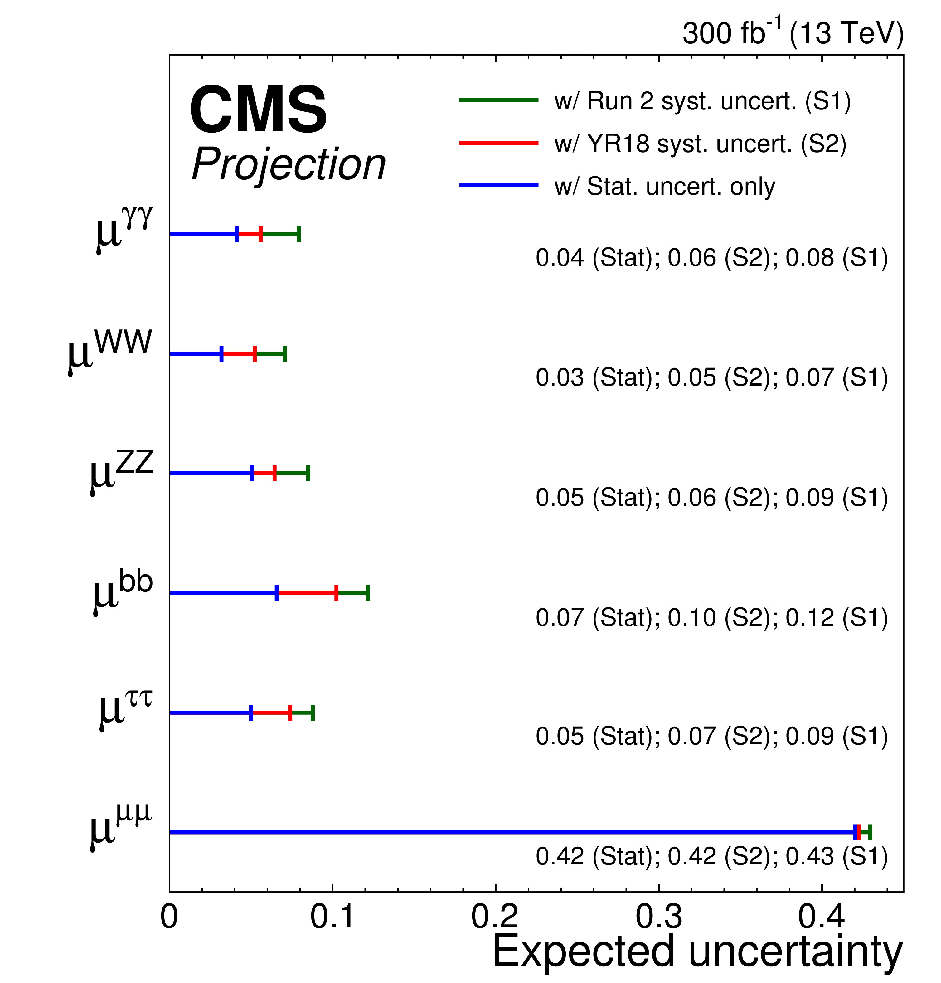
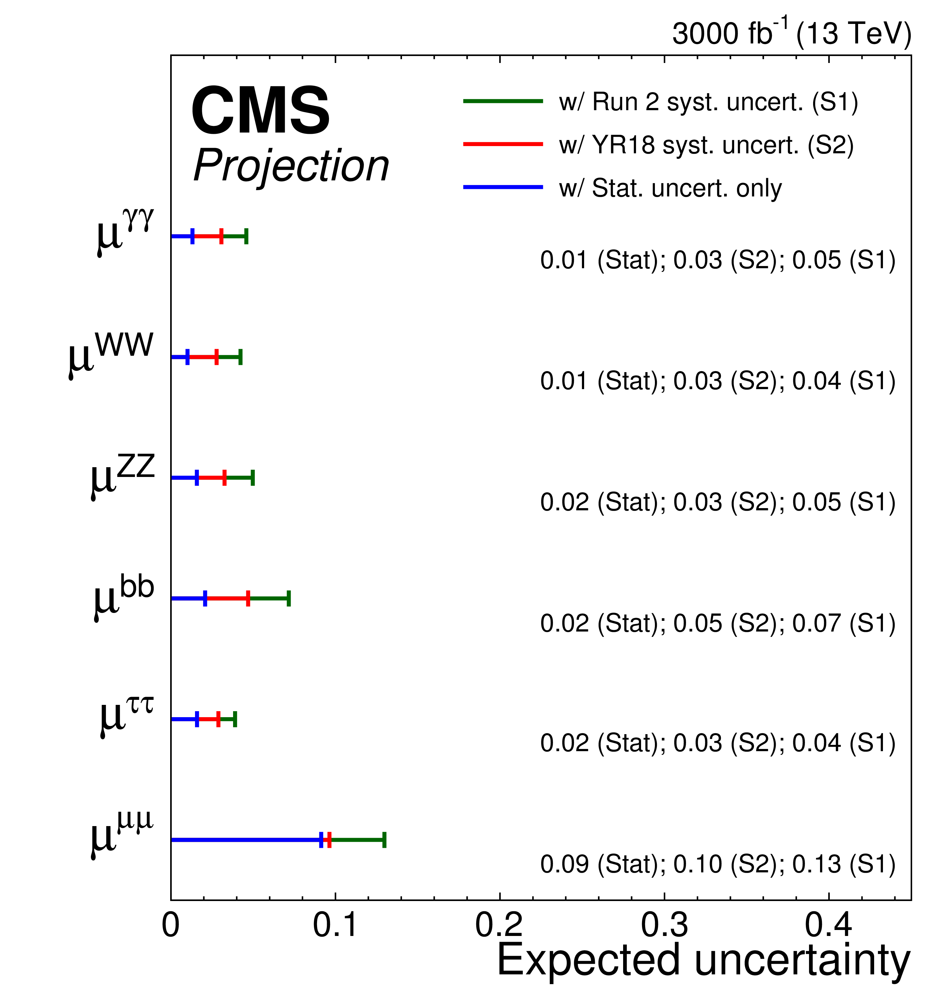
Figure 1:
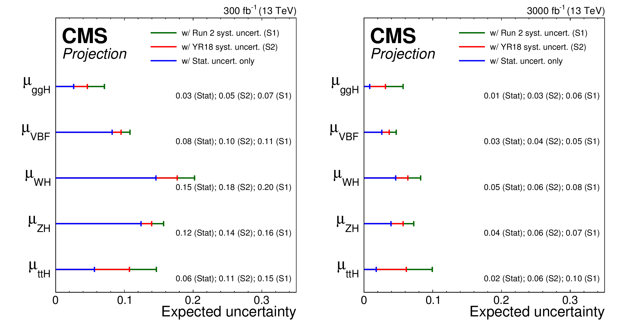
Summary plot showing the total expected $ \pm $1$ \sigma $ uncertainties in S1 (with Run 2 systematic uncertainties [30]) and S2 (with YR18 systematic uncertainties) on the per-decay-mode signal strength parameters for 300 fb$^{-1}$ (left) and 3000 fb$^{-1}$ (right). The statistical-only component of the uncertainty is also shown. |
png pdf |
Figure 1-a:
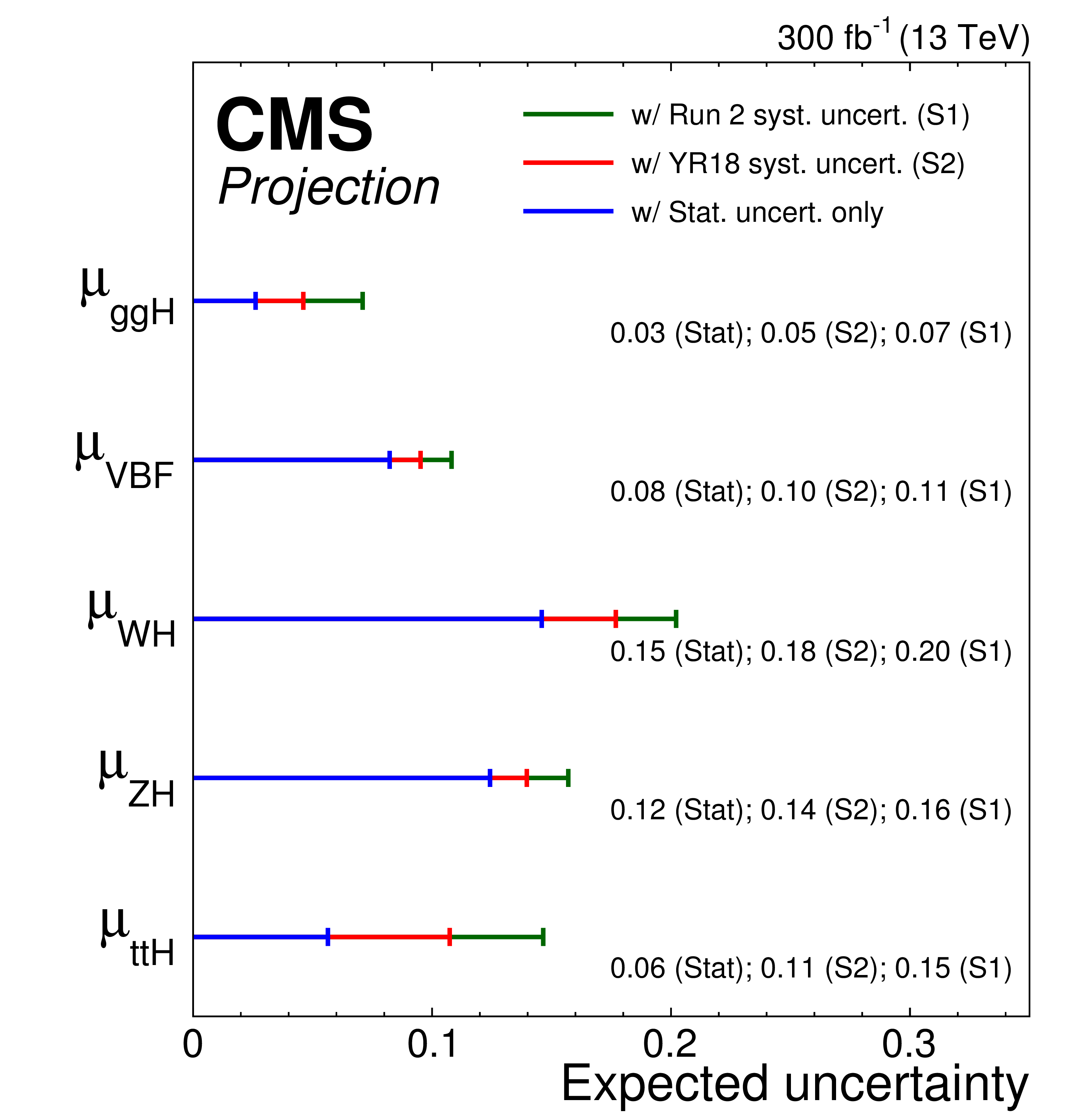
Summary plot showing the total expected $ \pm $1$ \sigma $ uncertainties in S1 (with Run 2 systematic uncertainties [30]) and S2 (with YR18 systematic uncertainties) on the per-decay-mode signal strength parameters for 300 fb$^{-1}$ (left) and 3000 fb$^{-1}$ (right). The statistical-only component of the uncertainty is also shown. |
png pdf |
Figure 1-b:
Summary plot showing the total expected $ \pm $1$ \sigma $ uncertainties in S1 (with Run 2 systematic uncertainties [30]) and S2 (with YR18 systematic uncertainties) on the per-decay-mode signal strength parameters for 300 fb$^{-1}$ (left) and 3000 fb$^{-1}$ (right). The statistical-only component of the uncertainty is also shown. |

png pdf |
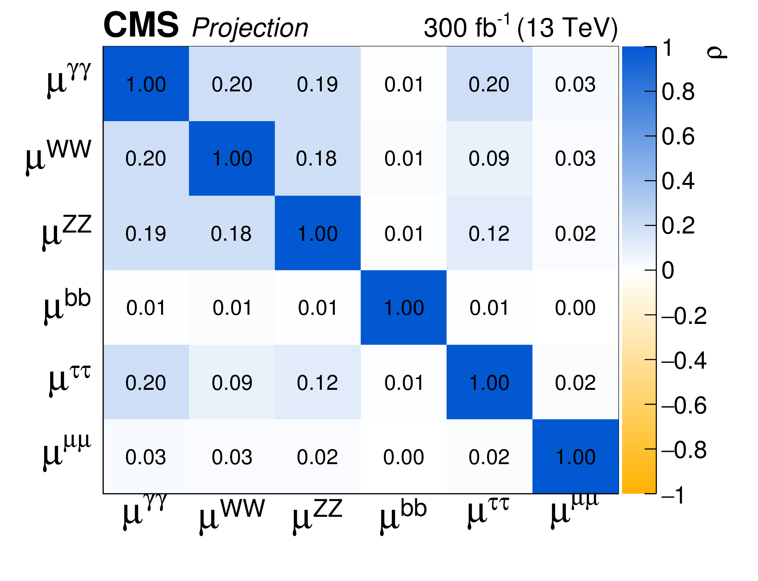
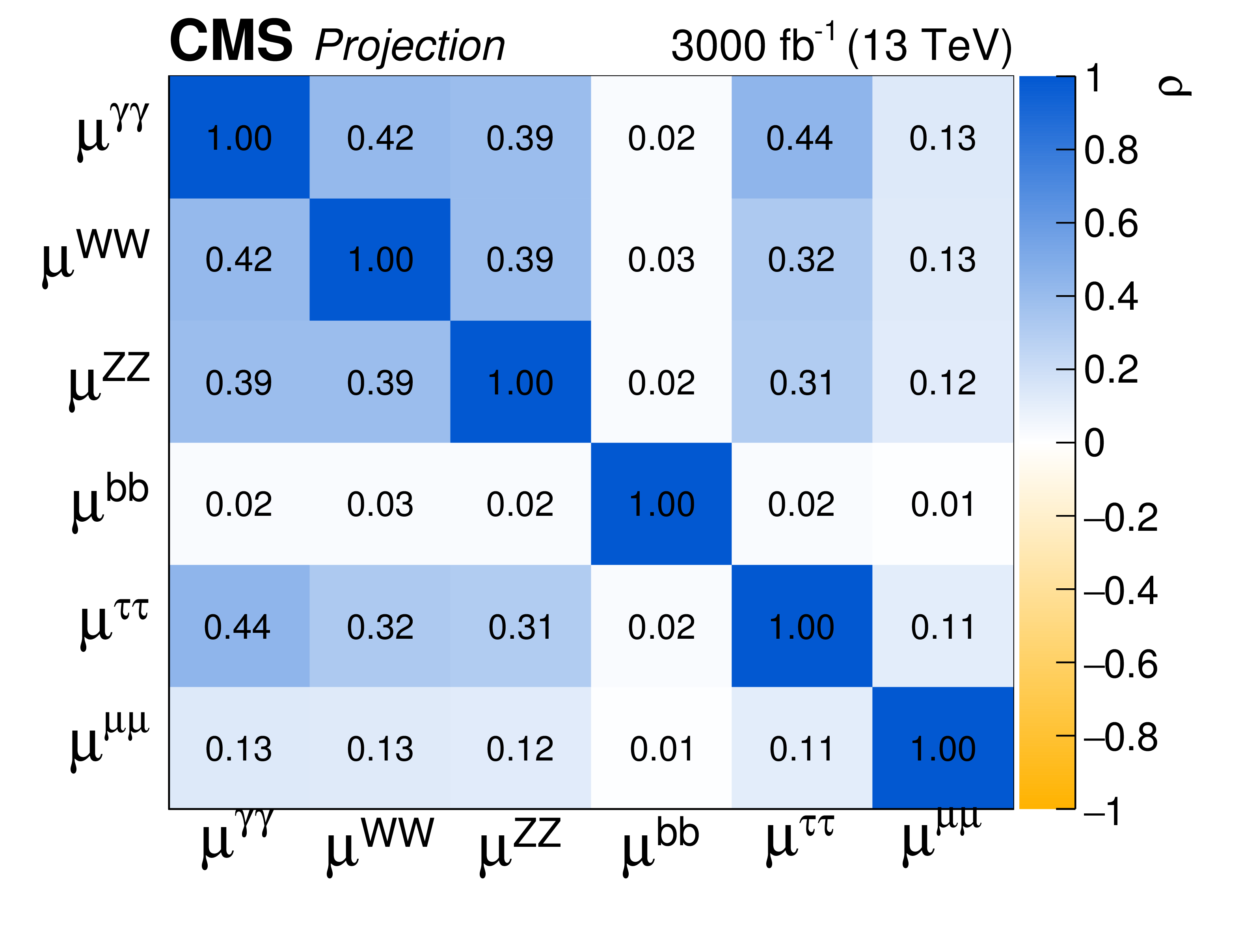
Figure 2:
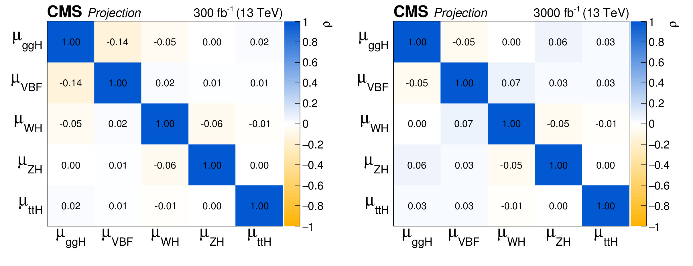
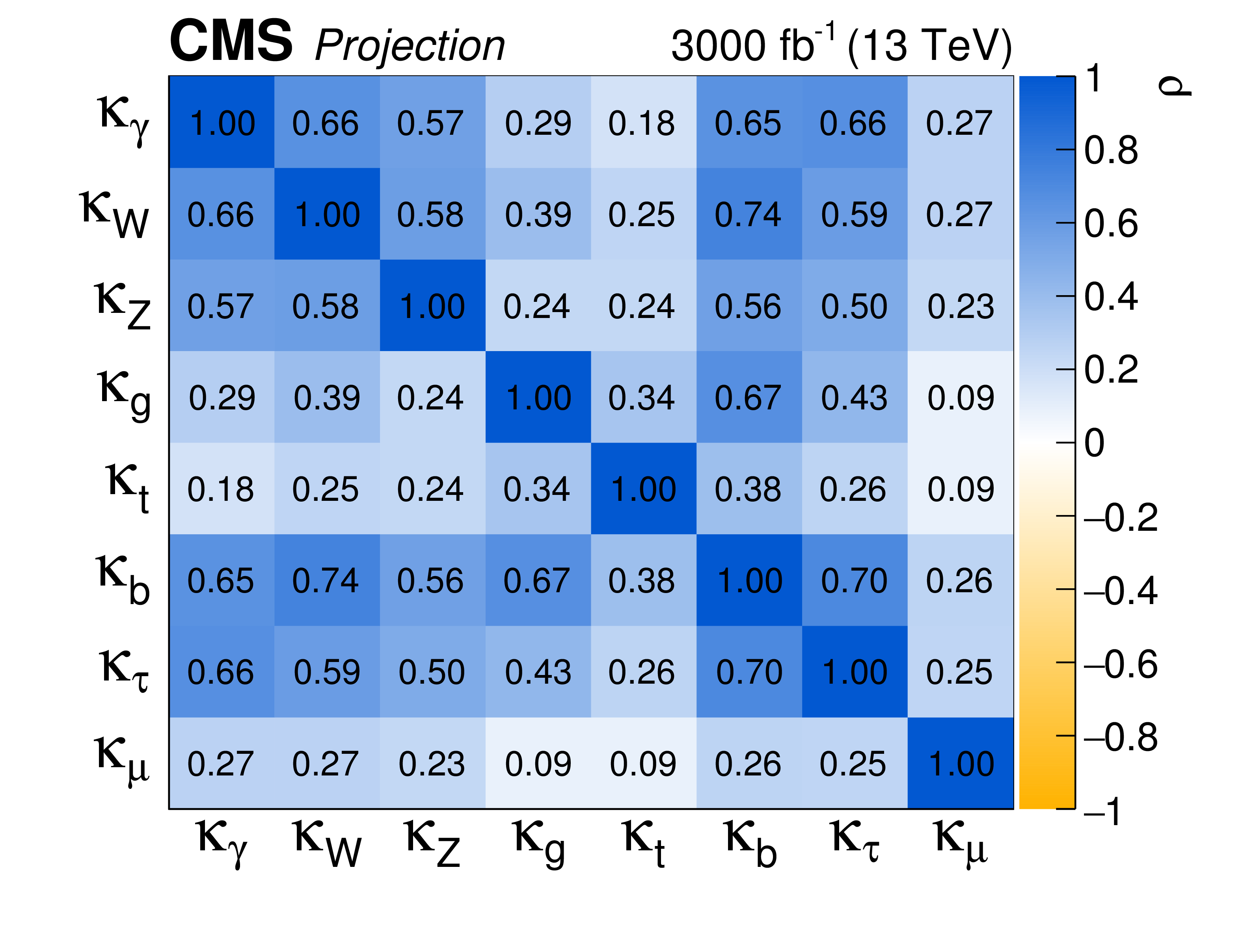
Correlation coefficients ($\rho $) between parameters in the signal strength per-decay-mode parametrisation for S2 (with YR18 systematic uncertainties) at 300 fb$^{-1}$ (left) and 3000 fb$^{-1}$ (right). |
png pdf |
Figure 2-a:
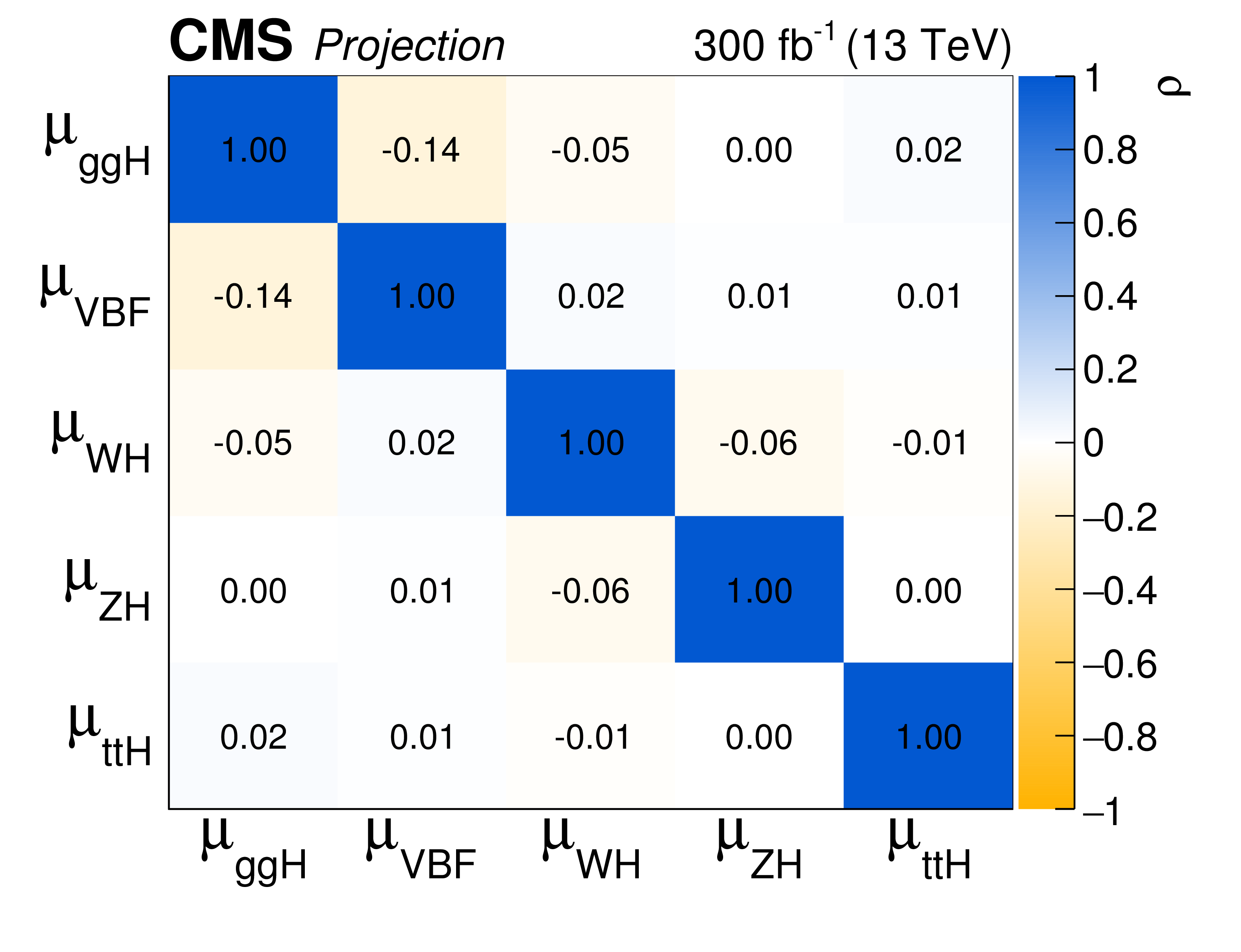
Correlation coefficients ($\rho $) between parameters in the signal strength per-decay-mode parametrisation for S2 (with YR18 systematic uncertainties) at 300 fb$^{-1}$ (left) and 3000 fb$^{-1}$ (right). |
png pdf |
Figure 2-b:
Correlation coefficients ($\rho $) between parameters in the signal strength per-decay-mode parametrisation for S2 (with YR18 systematic uncertainties) at 300 fb$^{-1}$ (left) and 3000 fb$^{-1}$ (right). |
png pdf |
Figure 3:
Summary plot showing the total expected $ \pm $1$ \sigma $ uncertainties in S1 (with Run 2 systematic uncertainties [30]) and S2 (with YR18 systematic uncertainties) on the per-production-mode signal strength parameters for 300 fb$^{-1}$ (left) and 3000 fb$^{-1}$ (right). The statistical-only component of the uncertainty is also shown. |
png pdf |
Figure 3-a:
Summary plot showing the total expected $ \pm $1$ \sigma $ uncertainties in S1 (with Run 2 systematic uncertainties [30]) and S2 (with YR18 systematic uncertainties) on the per-production-mode signal strength parameters for 300 fb$^{-1}$ (left) and 3000 fb$^{-1}$ (right). The statistical-only component of the uncertainty is also shown. |

png pdf |
Figure 3-b:
Summary plot showing the total expected $ \pm $1$ \sigma $ uncertainties in S1 (with Run 2 systematic uncertainties [30]) and S2 (with YR18 systematic uncertainties) on the per-production-mode signal strength parameters for 300 fb$^{-1}$ (left) and 3000 fb$^{-1}$ (right). The statistical-only component of the uncertainty is also shown. |
png pdf |
Figure 4:
Correlation coefficients ($\rho $) between parameters in the signal strength per-production-mode parametrisation for S2 (with YR18 systematic uncertainties) at 300 fb$^{-1}$ (left) and 3000 fb$^{-1}$ (right). |
png pdf |
Figure 4-a:
Correlation coefficients ($\rho $) between parameters in the signal strength per-production-mode parametrisation for S2 (with YR18 systematic uncertainties) at 300 fb$^{-1}$ (left) and 3000 fb$^{-1}$ (right). |

png pdf |
Figure 4-b:
Correlation coefficients ($\rho $) between parameters in the signal strength per-production-mode parametrisation for S2 (with YR18 systematic uncertainties) at 300 fb$^{-1}$ (left) and 3000 fb$^{-1}$ (right). |
png pdf |
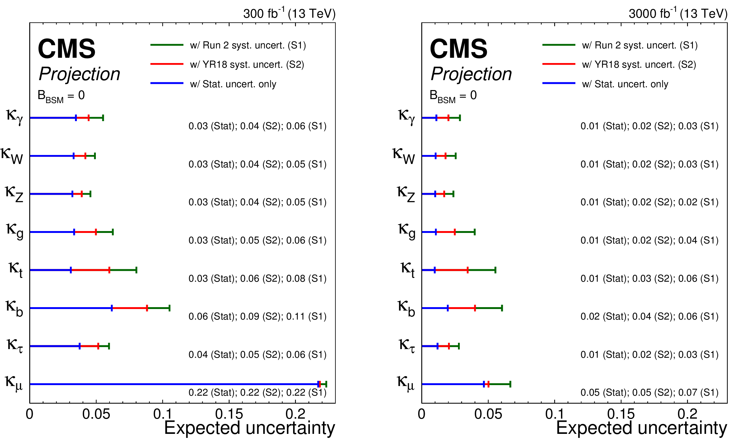
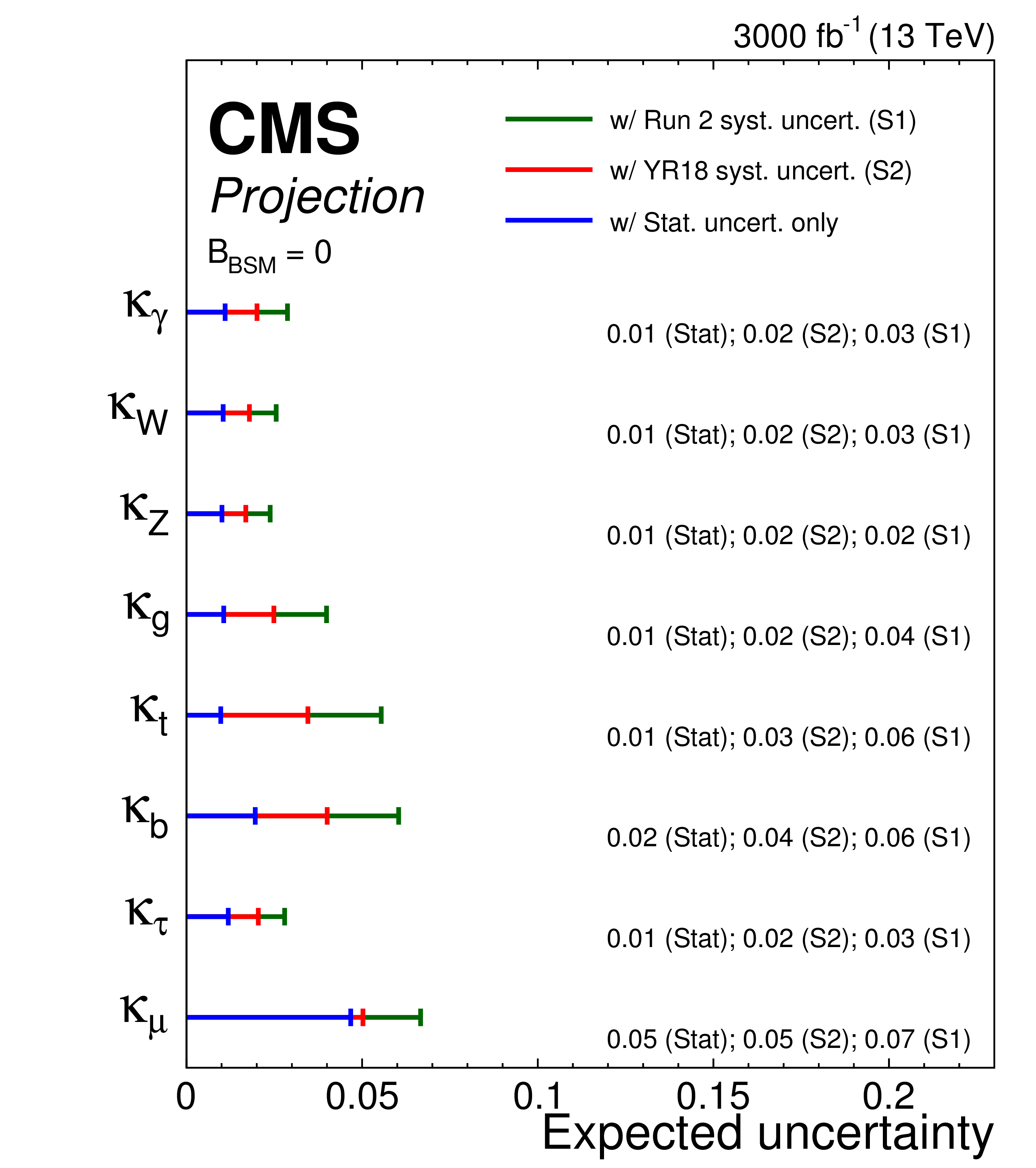
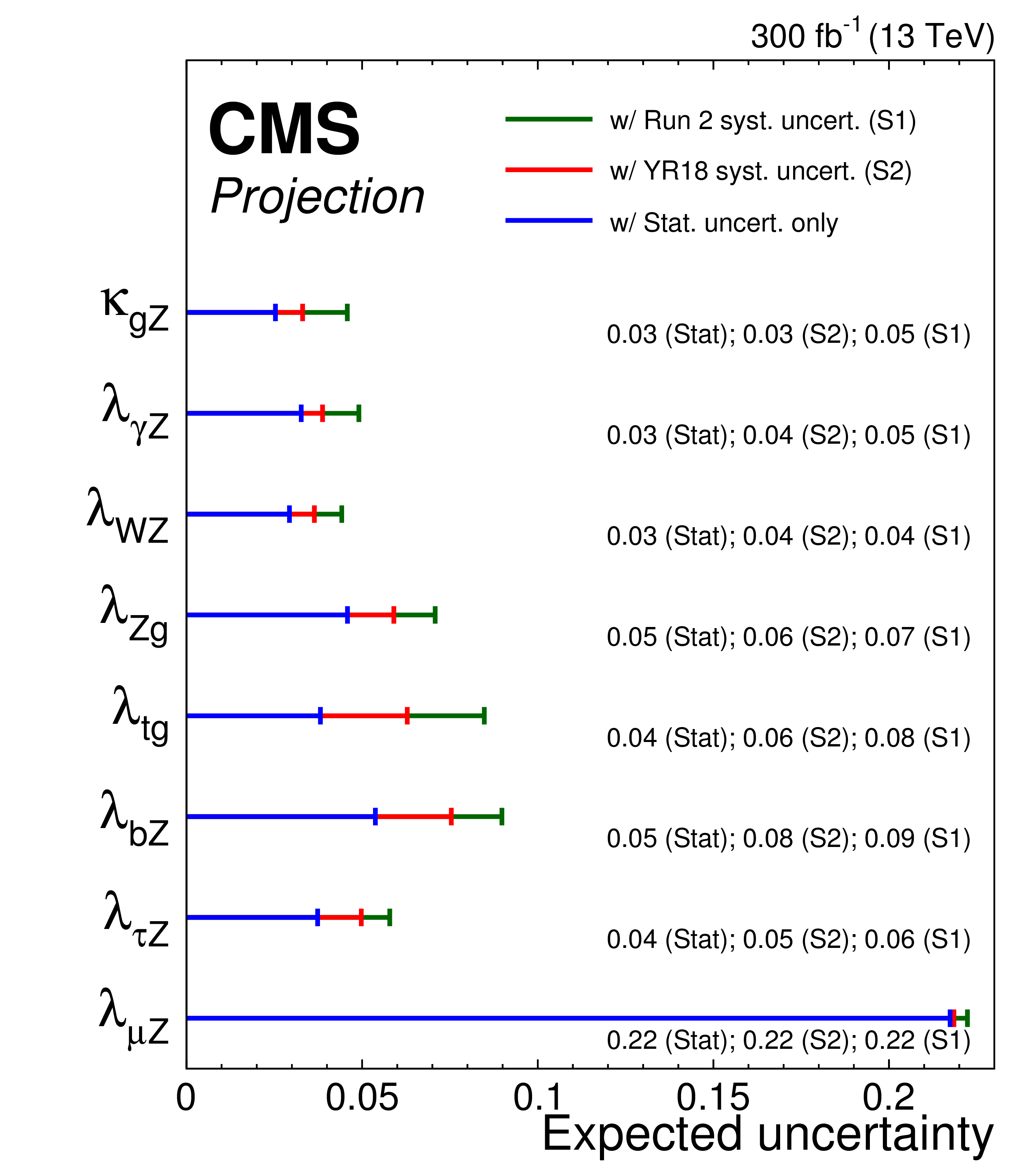
Figure 5:
Summary plot showing the total expected $ \pm $1$ \sigma $ uncertainties in S1 (with Run 2 systematic uncertainties [30]) and S2 (with YR18 systematic uncertainties) on the coupling modifier parameters for 300 fb$^{-1}$ (left) and 3000 fb$^{-1}$ (right). The statistical-only component of the uncertainty is also shown. |

png pdf |
Figure 5-a:
Summary plot showing the total expected $ \pm $1$ \sigma $ uncertainties in S1 (with Run 2 systematic uncertainties [30]) and S2 (with YR18 systematic uncertainties) on the coupling modifier parameters for 300 fb$^{-1}$ (left) and 3000 fb$^{-1}$ (right). The statistical-only component of the uncertainty is also shown. |
png pdf |
Figure 5-b:
Summary plot showing the total expected $ \pm $1$ \sigma $ uncertainties in S1 (with Run 2 systematic uncertainties [30]) and S2 (with YR18 systematic uncertainties) on the coupling modifier parameters for 300 fb$^{-1}$ (left) and 3000 fb$^{-1}$ (right). The statistical-only component of the uncertainty is also shown. |
png pdf |
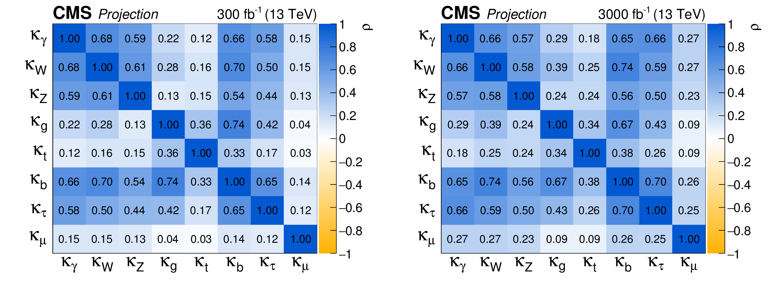
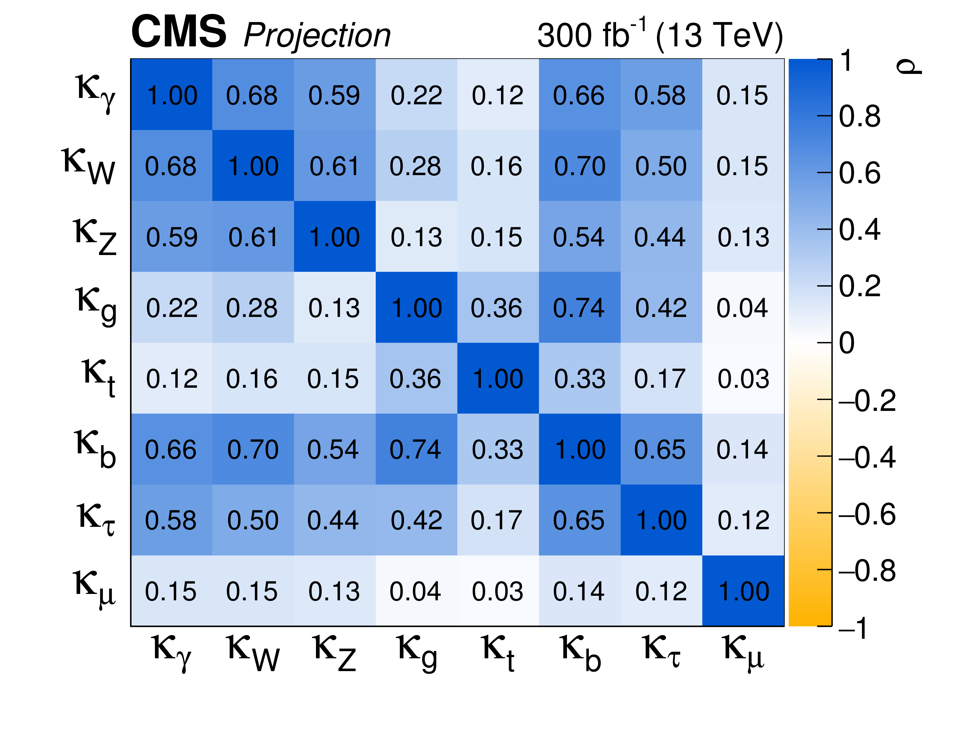
Figure 6:
Correlation coefficients ($\rho $) between parameters in the coupling modifier parametrisation for S2 (with YR18 systematic uncertainties) at 300 fb$^{-1}$ (left) and 3000 fb$^{-1}$ (right). |
png pdf |
Figure 6-a:
Correlation coefficients ($\rho $) between parameters in the coupling modifier parametrisation for S2 (with YR18 systematic uncertainties) at 300 fb$^{-1}$ (left) and 3000 fb$^{-1}$ (right). |
png pdf |
Figure 6-b:
Correlation coefficients ($\rho $) between parameters in the coupling modifier parametrisation for S2 (with YR18 systematic uncertainties) at 300 fb$^{-1}$ (left) and 3000 fb$^{-1}$ (right). |
png pdf |
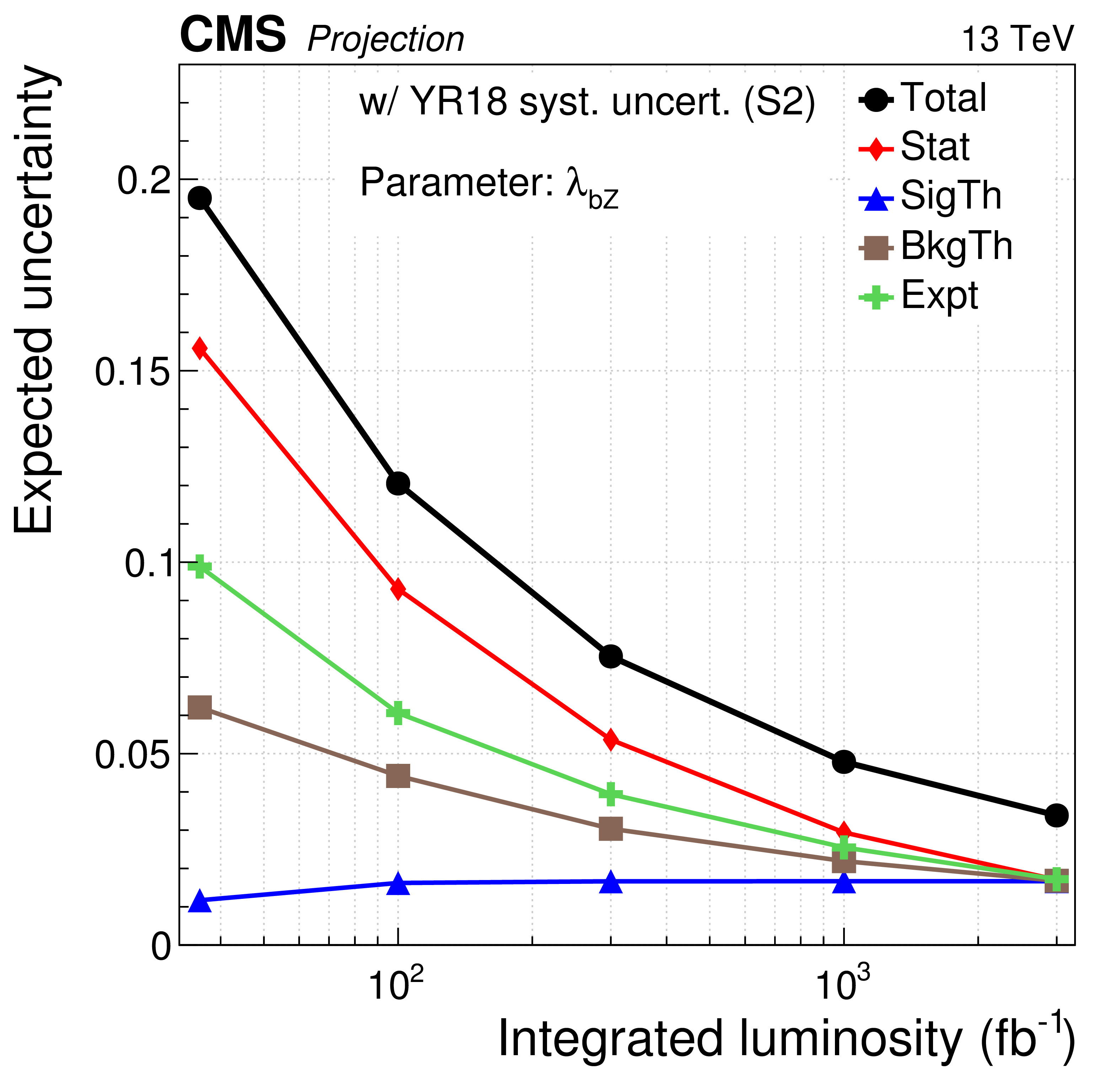
Figure 7:
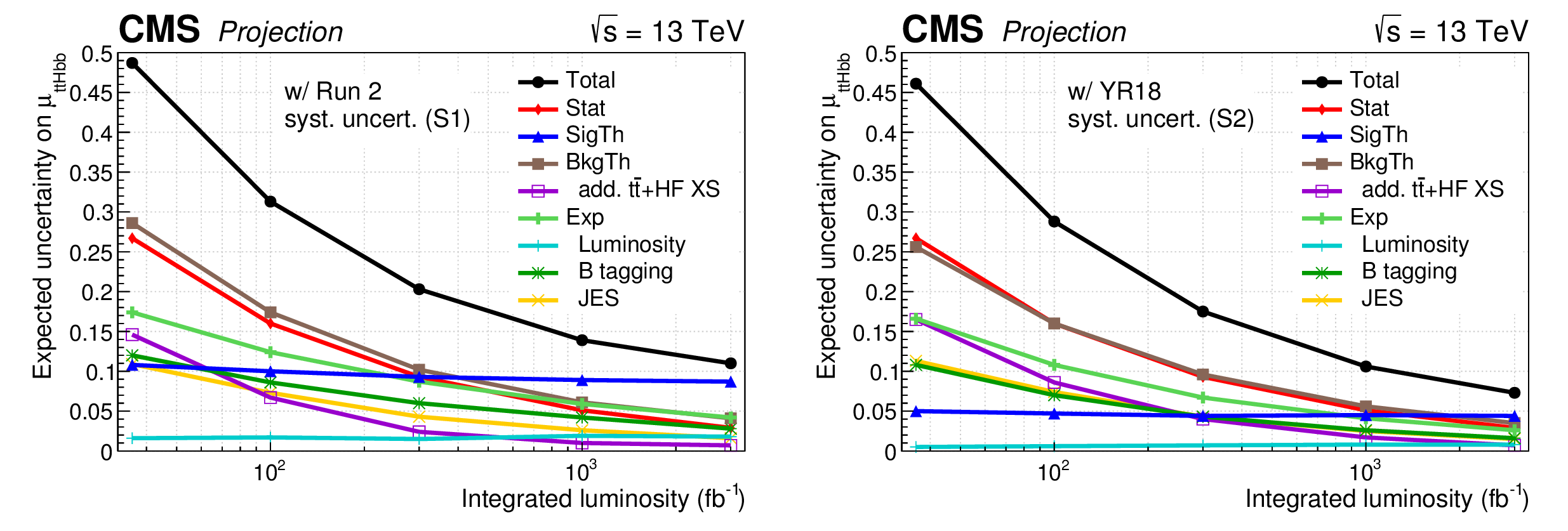
Expected uncertainties on the ttH signal strength as a function of the integrated luminosity under the S1 (left, with Run 2 systematic uncertainties [27]) and S2 (right, with YR18 systematic uncertainties) scenarios. Shown are the total uncertainty (black) and contributions of different groups of uncertainties. Results with 35.9 fb$^{-1}$ are intended for comparison with the projections to higher luminosities and differ in parts from [27] for consistency with the projected results: uncertainties due to the limited number of MC events have been omitted and theory systematic uncertainties have been halved in case of the scenario S2. |

png pdf |
Figure 7-a:
Expected uncertainties on the ttH signal strength as a function of the integrated luminosity under the S1 (left, with Run 2 systematic uncertainties [27]) and S2 (right, with YR18 systematic uncertainties) scenarios. Shown are the total uncertainty (black) and contributions of different groups of uncertainties. Results with 35.9 fb$^{-1}$ are intended for comparison with the projections to higher luminosities and differ in parts from [27] for consistency with the projected results: uncertainties due to the limited number of MC events have been omitted and theory systematic uncertainties have been halved in case of the scenario S2. |
png pdf |
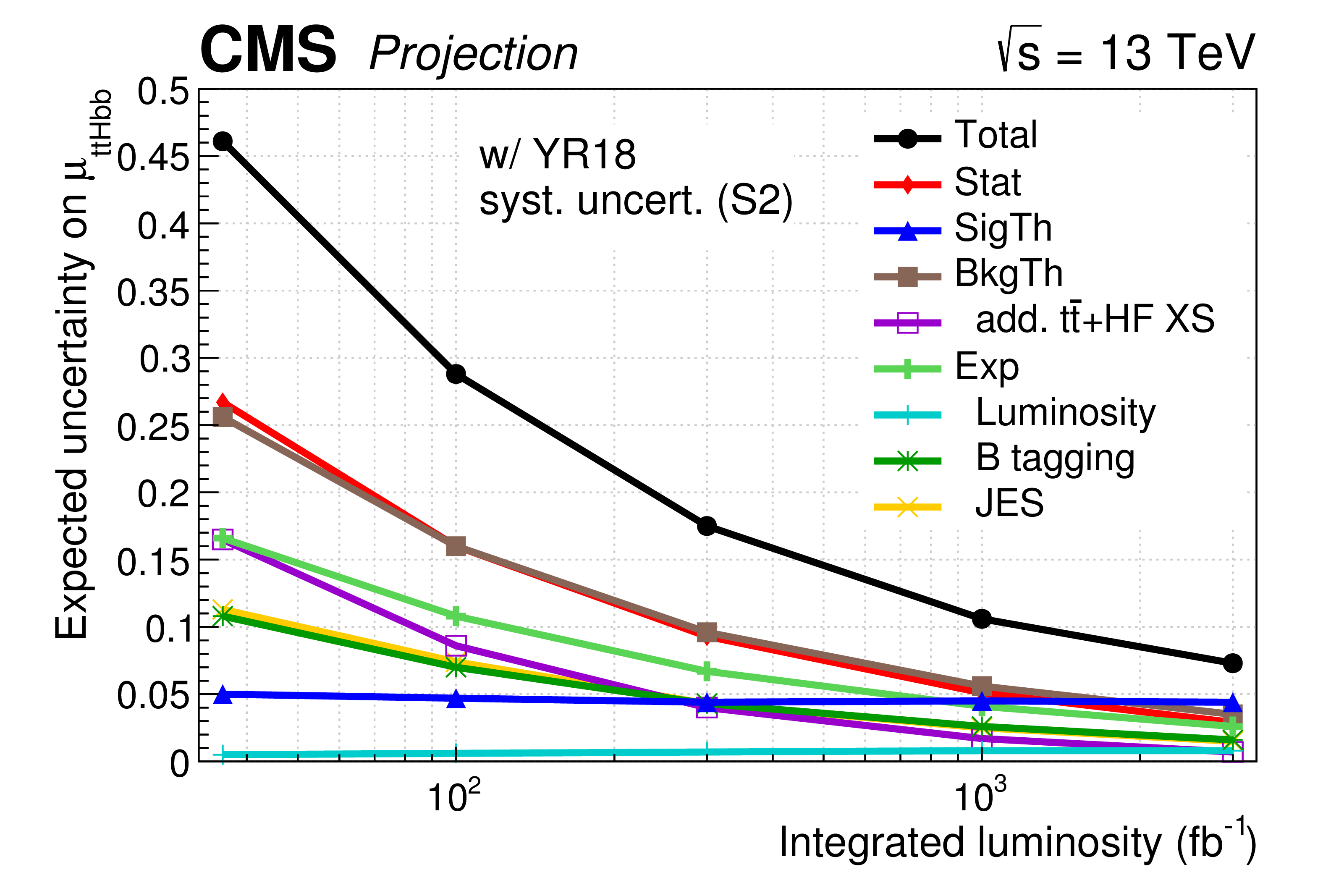
Figure 7-b:
Expected uncertainties on the ttH signal strength as a function of the integrated luminosity under the S1 (left, with Run 2 systematic uncertainties [27]) and S2 (right, with YR18 systematic uncertainties) scenarios. Shown are the total uncertainty (black) and contributions of different groups of uncertainties. Results with 35.9 fb$^{-1}$ are intended for comparison with the projections to higher luminosities and differ in parts from [27] for consistency with the projected results: uncertainties due to the limited number of MC events have been omitted and theory systematic uncertainties have been halved in case of the scenario S2. |
png pdf |
Figure 8:
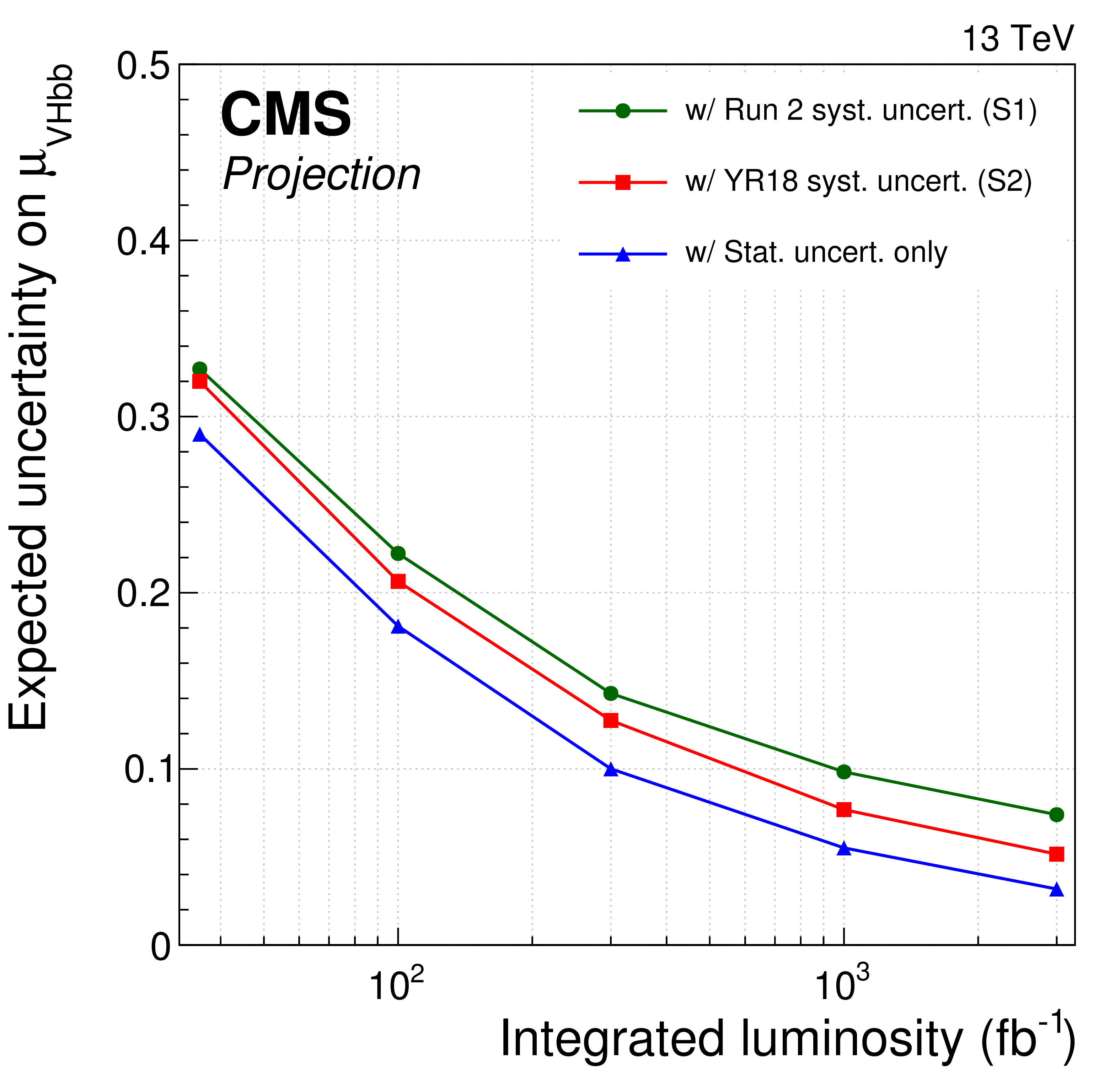
Uncertainty on the signal strength $\mu _{\text {VHbb}}$ as a function of integrated luminosity for S1 (with Run 2 systematic uncertainties [24]) and S2 (with YR18 systematic uncertainties). Results with 35.9 fb$^{-1}$ are intended for comparison with the projections to higher luminosities and differ in parts from [24] for consistency with the projected results: uncertainties due to the limited number of MC events have been omitted and theory systematic uncertainties have been halved in case of the scenario S2. |
png pdf |
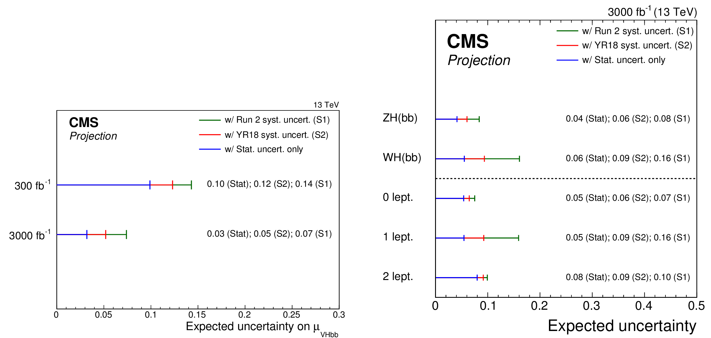
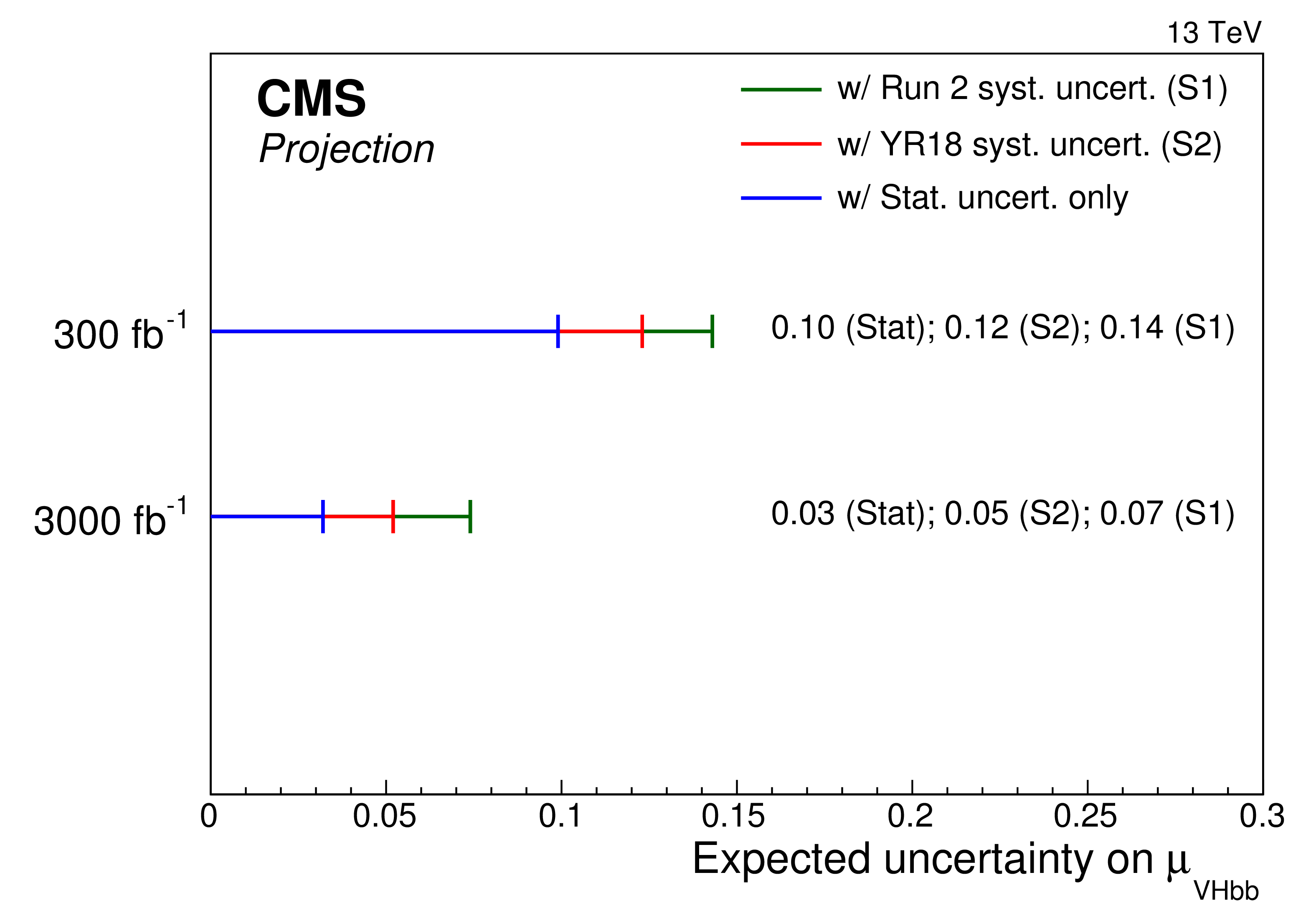
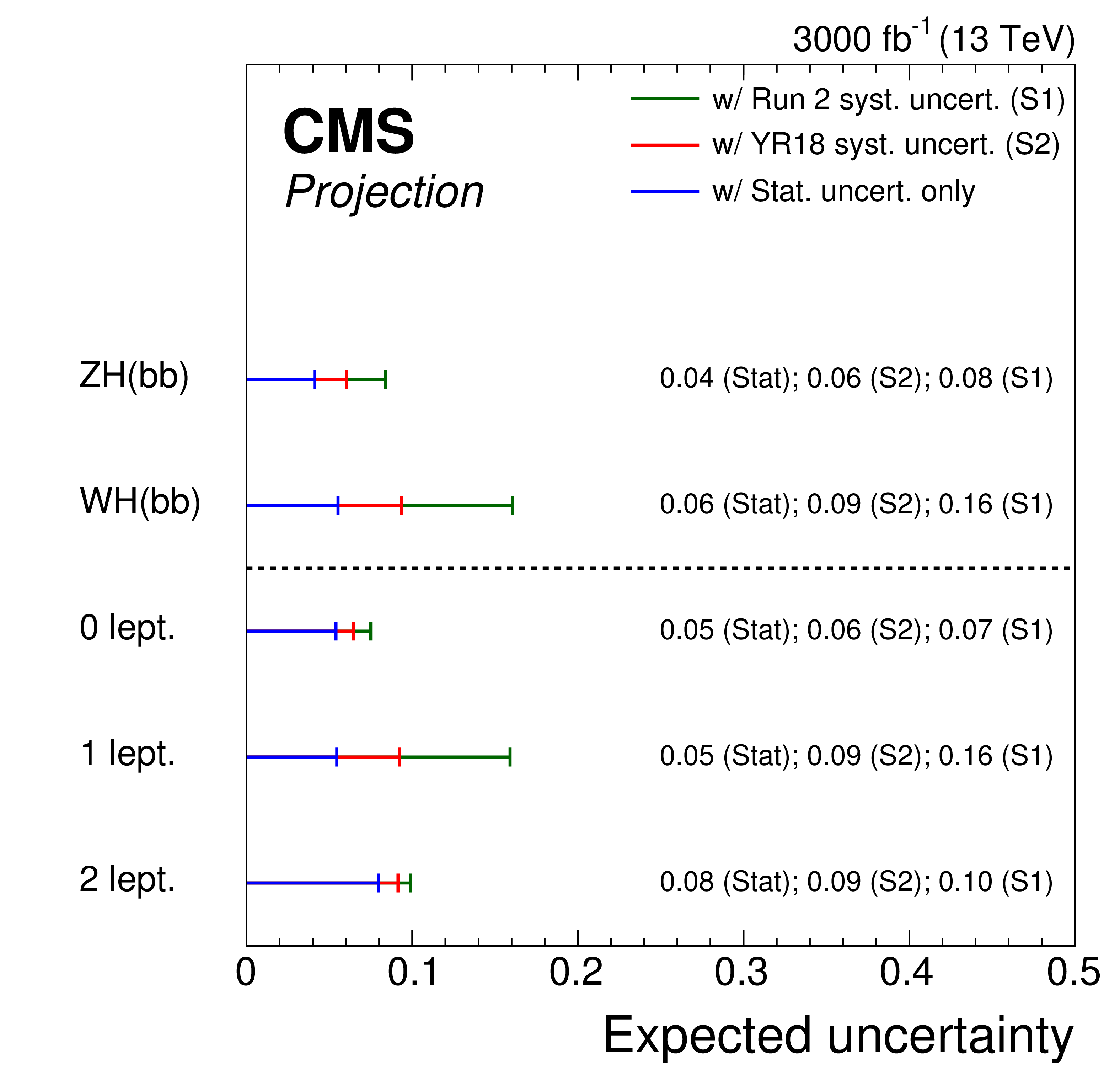
Figure 9:
Uncertainties in the overall signal strength $\mu _{\text {VHbb}}$ at 300 and 3000 fb$^{-1}$ (left) and per-process and per-channel signal strengths at 3000 fb$^{-1}$ (right). Values are given for the S1 (with Run 2 systematic uncertainties [24]) and S2 (with YR18 systematic uncertainties) scenarios, as well as a scenario in which all systematic uncertainties are removed. |
png pdf |
Figure 9-a:
Uncertainties in the overall signal strength $\mu _{\text {VHbb}}$ at 300 and 3000 fb$^{-1}$ (left) and per-process and per-channel signal strengths at 3000 fb$^{-1}$ (right). Values are given for the S1 (with Run 2 systematic uncertainties [24]) and S2 (with YR18 systematic uncertainties) scenarios, as well as a scenario in which all systematic uncertainties are removed. |
png pdf |
Figure 9-b:
Uncertainties in the overall signal strength $\mu _{\text {VHbb}}$ at 300 and 3000 fb$^{-1}$ (left) and per-process and per-channel signal strengths at 3000 fb$^{-1}$ (right). Values are given for the S1 (with Run 2 systematic uncertainties [24]) and S2 (with YR18 systematic uncertainties) scenarios, as well as a scenario in which all systematic uncertainties are removed. |

png pdf |
Figure 10:
Effect of varying the b tagging efficiency ($\varepsilon ^{\text {b-tag}}$) on the uncertainty in the signal strength measurement when considering all systematic uncertainties. |
png pdf |
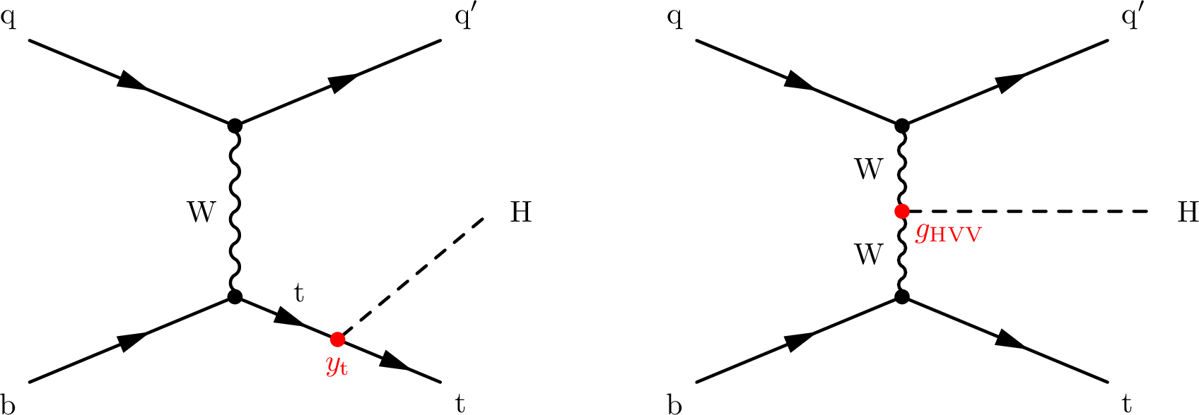
Figure 11:
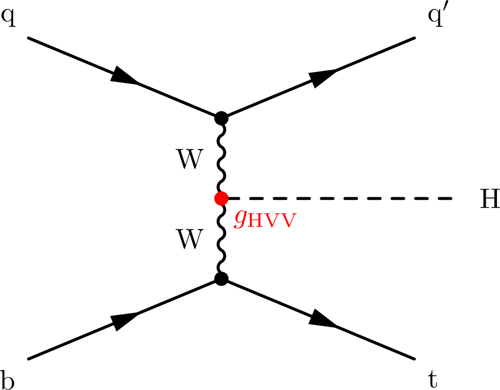
The representative leading-order diagrams for tHq production. |

png pdf |
Figure 11-a:
The representative leading-order diagrams for tHq production. |
png pdf |
Figure 11-b:
The representative leading-order diagrams for tHq production. |

png pdf |
Figure 12:
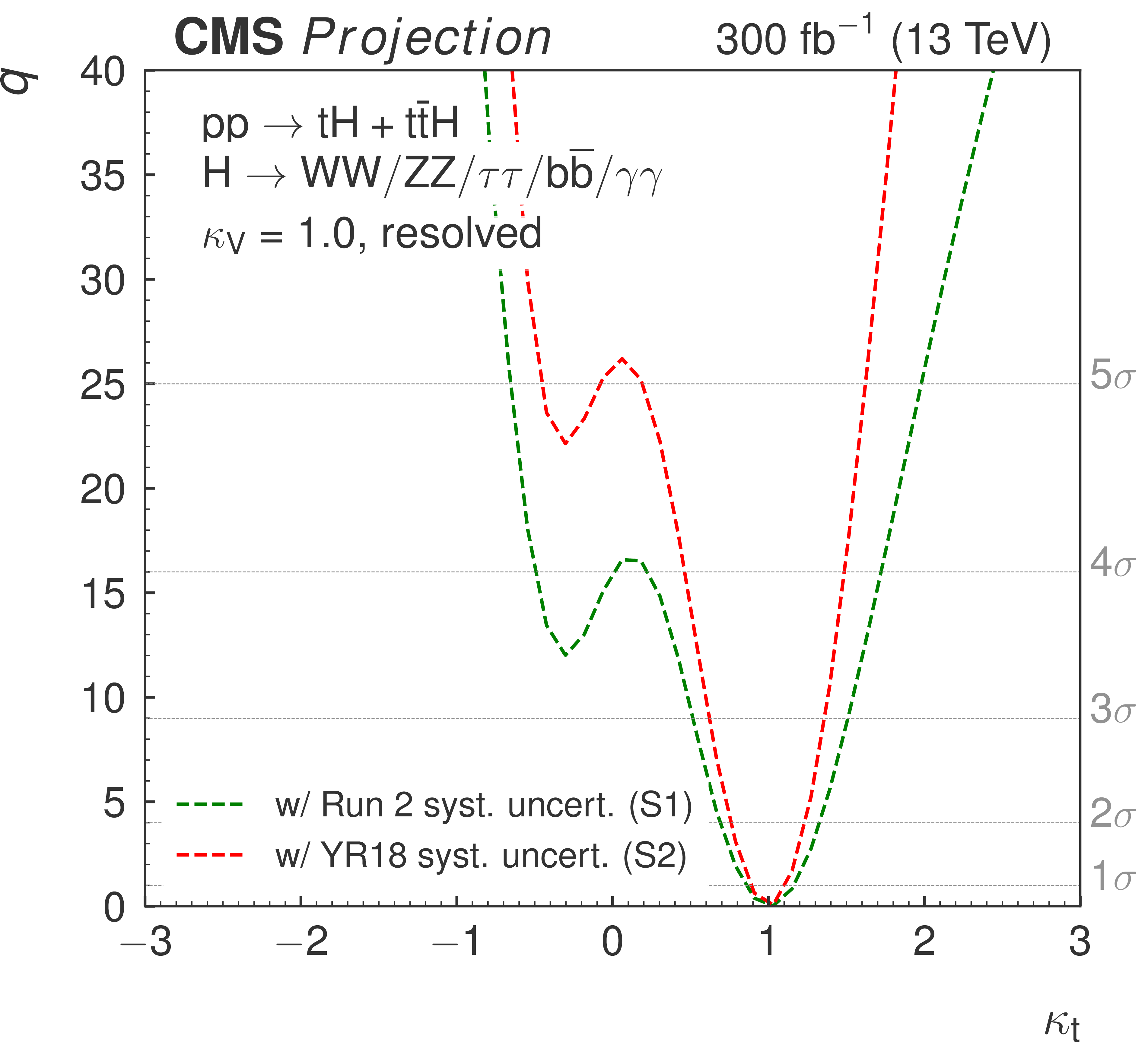
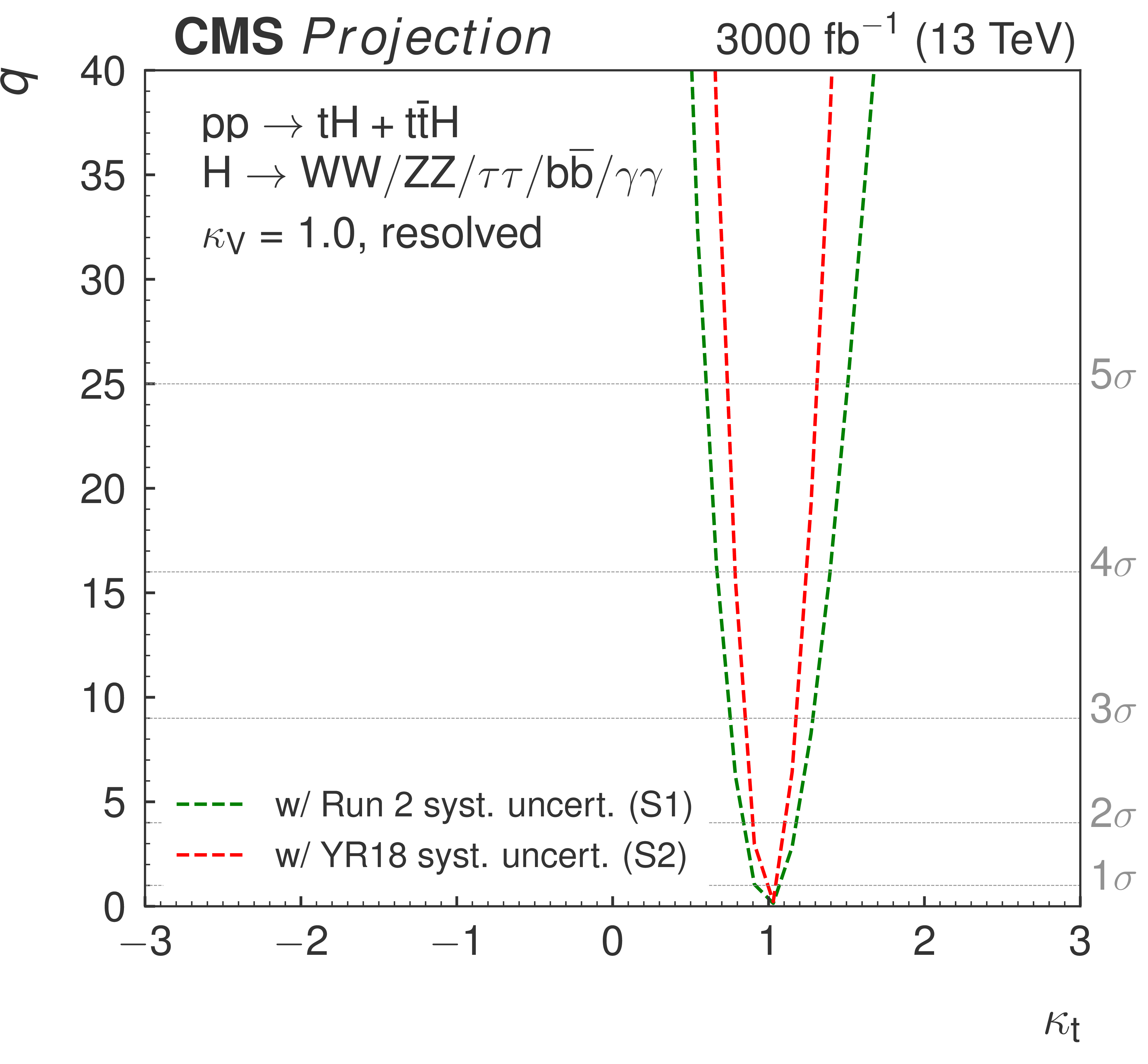
Scan of the test statistic $q$ versus $ {\kappa _{{\mathrm {t}}}} $ for the Asimov data sets corresponding to $ {\kappa _{\mathrm {V}}} =$ 1 for the two integrated luminosity scenarios in S1 (with Run 2 systematic uncertainties [38]) and S2 (with YR18 systematic uncertainties). |
png pdf |
Figure 12-a:
Scan of the test statistic $q$ versus $ {\kappa _{{\mathrm {t}}}} $ for the Asimov data sets corresponding to $ {\kappa _{\mathrm {V}}} =$ 1 for the two integrated luminosity scenarios in S1 (with Run 2 systematic uncertainties [38]) and S2 (with YR18 systematic uncertainties). |
png pdf |
Figure 12-b:
Scan of the test statistic $q$ versus $ {\kappa _{{\mathrm {t}}}} $ for the Asimov data sets corresponding to $ {\kappa _{\mathrm {V}}} =$ 1 for the two integrated luminosity scenarios in S1 (with Run 2 systematic uncertainties [38]) and S2 (with YR18 systematic uncertainties). |
png pdf |
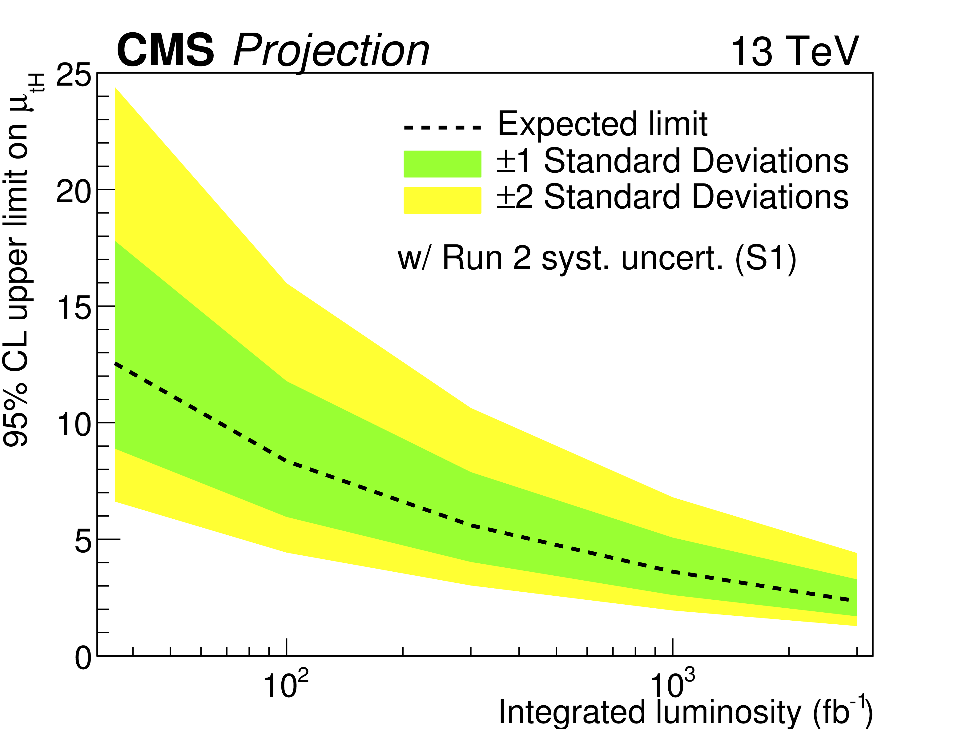
Figure 13:
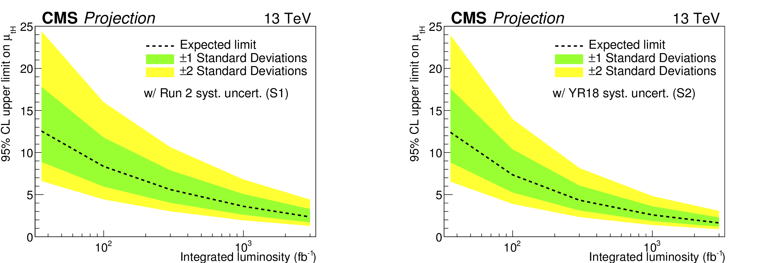
The variation of expected upper limit on $\mu _{{{\mathrm {t}} {\mathrm {H}}}}$ with integrated luminosity for two projection scenarios S1 (with Run 2 systematic uncertainties [38]) and S2 (with YR18 systematic uncertainties). |
png pdf |
Figure 13-a:
The variation of expected upper limit on $\mu _{{{\mathrm {t}} {\mathrm {H}}}}$ with integrated luminosity for two projection scenarios S1 (with Run 2 systematic uncertainties [38]) and S2 (with YR18 systematic uncertainties). |
png pdf |
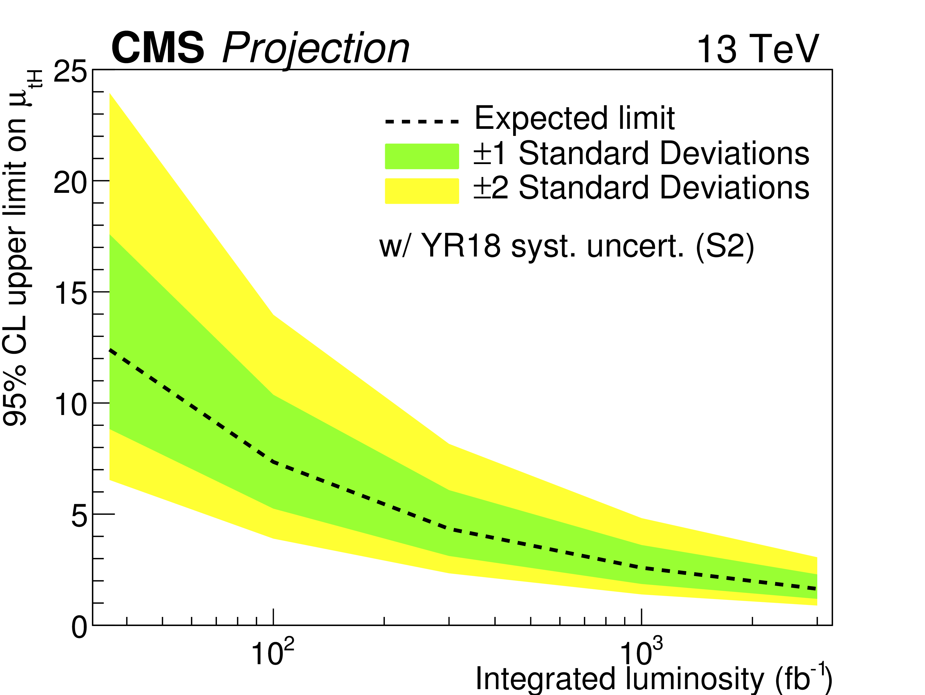
Figure 13-b:
The variation of expected upper limit on $\mu _{{{\mathrm {t}} {\mathrm {H}}}}$ with integrated luminosity for two projection scenarios S1 (with Run 2 systematic uncertainties [38]) and S2 (with YR18 systematic uncertainties). |

png pdf |
Figure 14:
Projected differential cross section for the $ {{p_{\mathrm {T}}} ({\mathrm {H}})} $ spectrum at an integrated luminosity of 3000 fb$^{-1}$, under S1 (left, with Run 2 systematic uncertainties [41]) and S2 (right, with YR18 systematic uncertainties). |
png pdf |
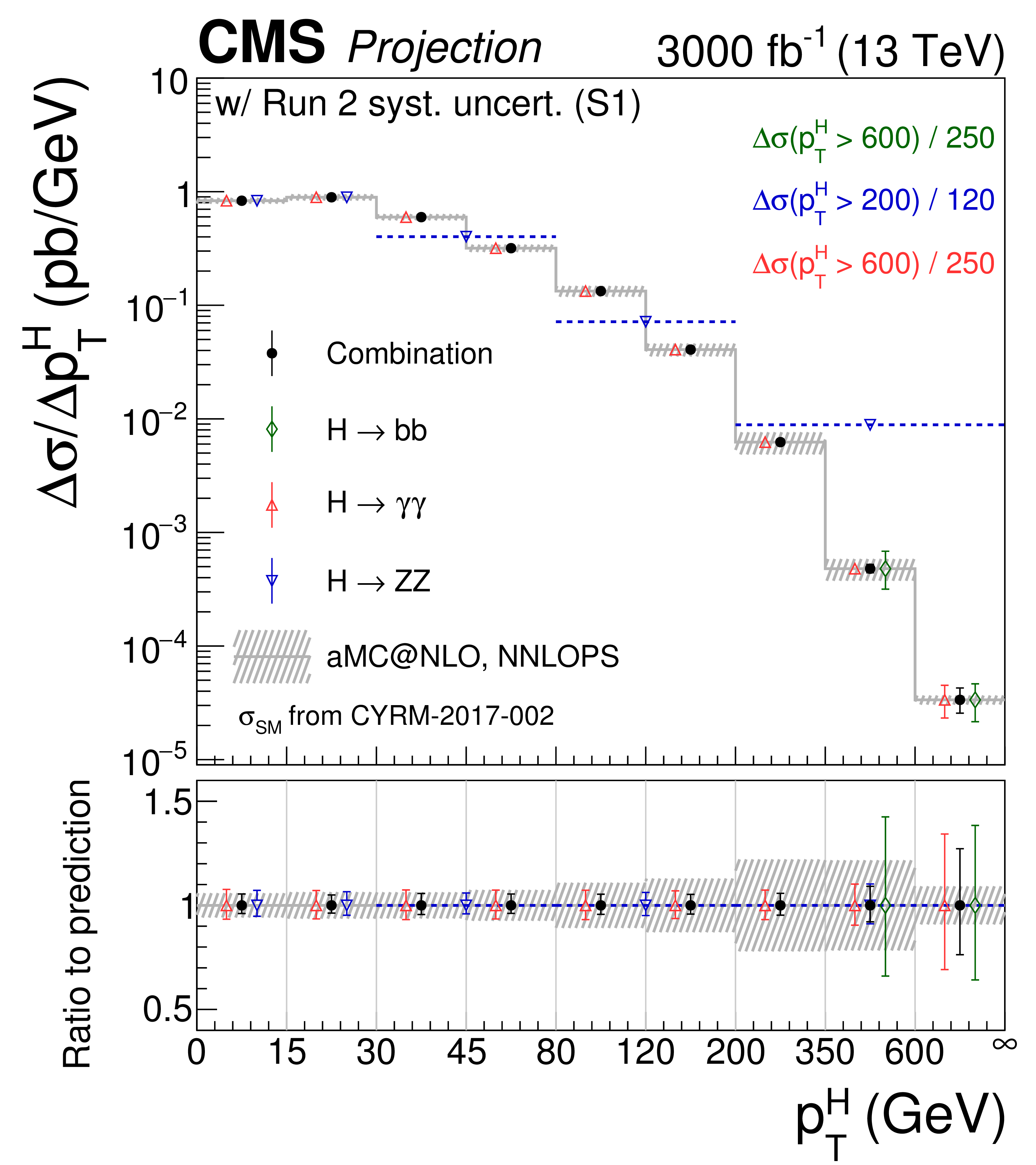
Figure 14-a:
Projected differential cross section for the $ {{p_{\mathrm {T}}} ({\mathrm {H}})} $ spectrum at an integrated luminosity of 3000 fb$^{-1}$, under S1 (left, with Run 2 systematic uncertainties [41]) and S2 (right, with YR18 systematic uncertainties). |
png pdf |
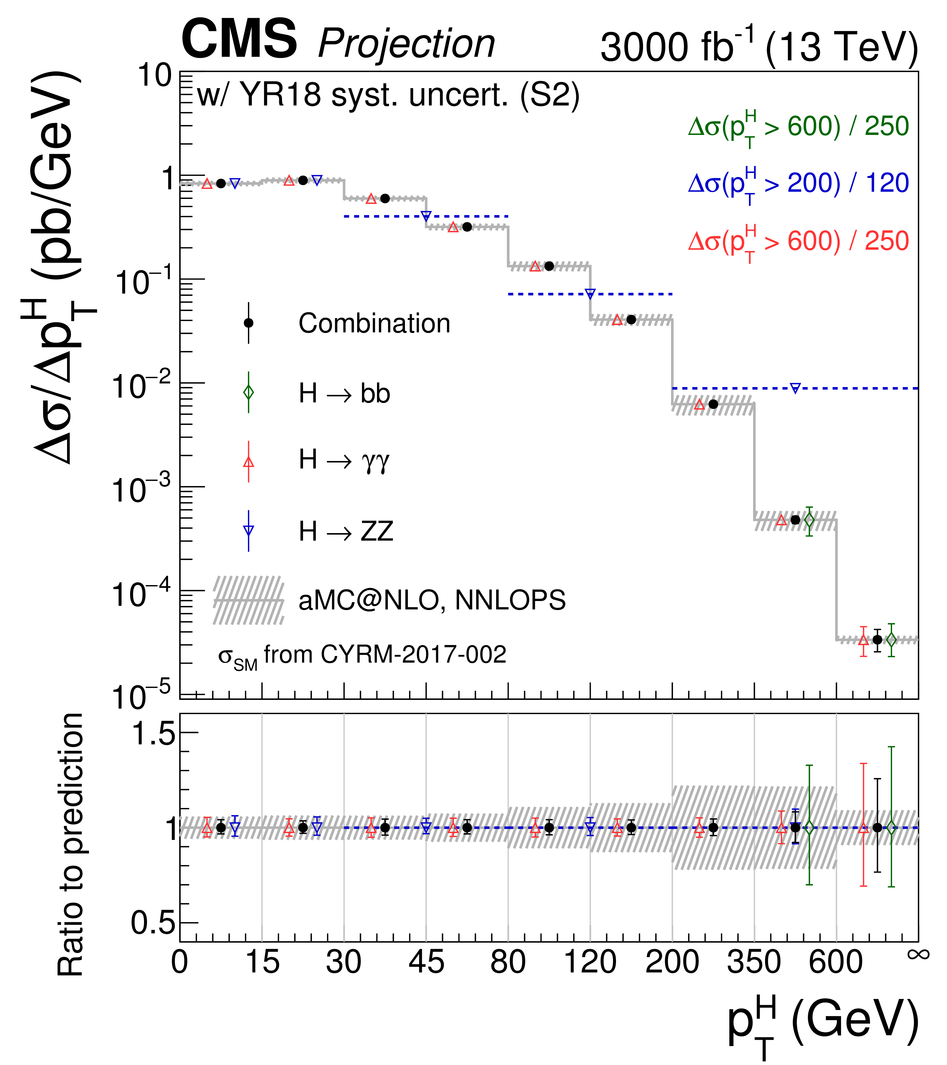
Figure 14-b:
Projected differential cross section for the $ {{p_{\mathrm {T}}} ({\mathrm {H}})} $ spectrum at an integrated luminosity of 3000 fb$^{-1}$, under S1 (left, with Run 2 systematic uncertainties [41]) and S2 (right, with YR18 systematic uncertainties). |

png pdf |
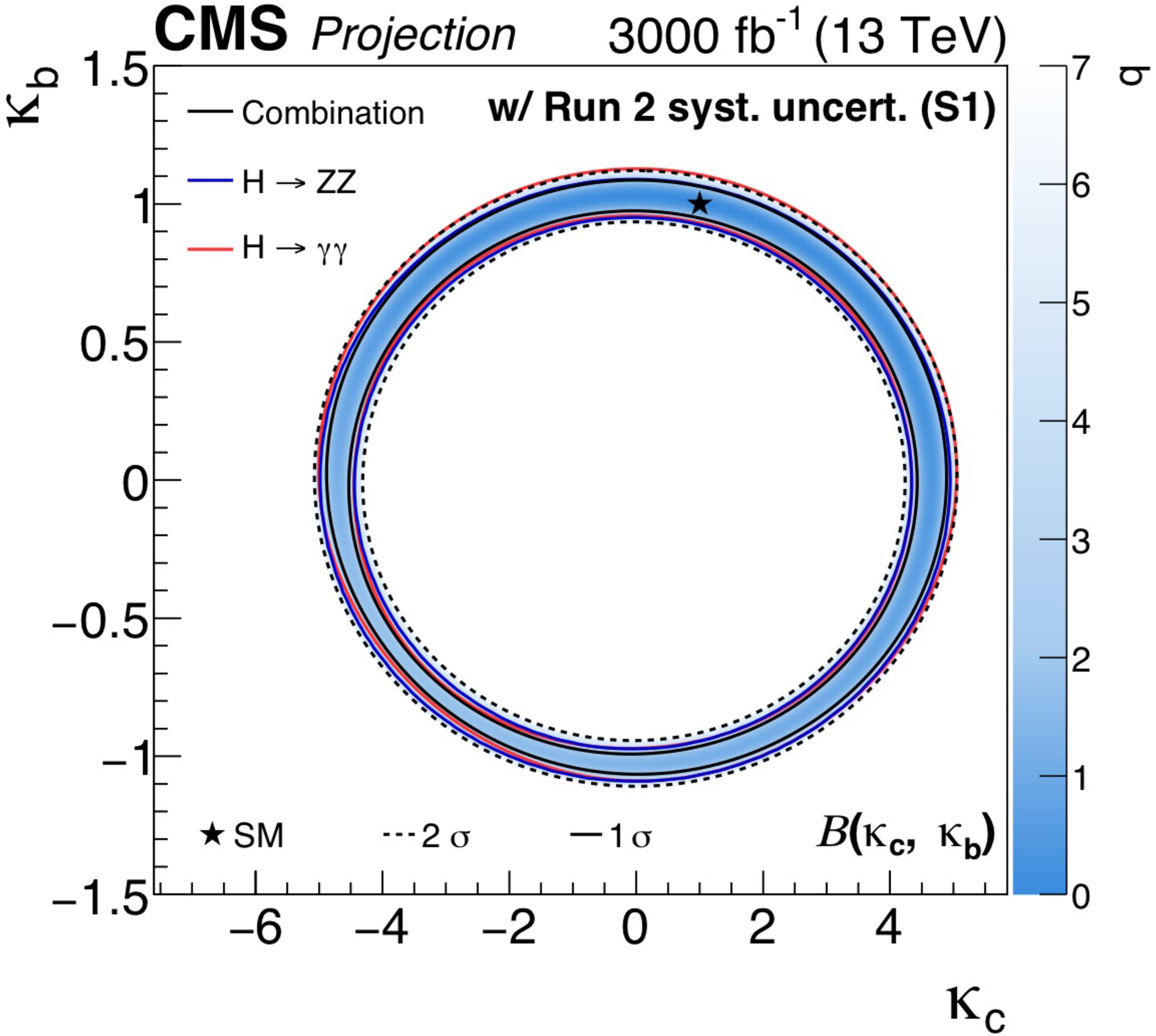
Figure 15:
Projected simultaneous fit for $\kappa _\textrm {b}$ and $\kappa _\textrm {c}$, assuming the branching fractions to be determined by the couplings (left) and the branching fractions implemented as nuisance parameters with no prior constraint (right), under S1 (top) and S2 (bottom). The one standard deviation contour is drawn for the combination ($ {{\mathrm {H}} \to {\gamma \gamma}} $ and $ {{\mathrm {H}} \to {{\mathrm {Z}} {\mathrm {Z}}}} $), the $ {{\mathrm {H}} \to {\gamma \gamma}} $ channel, and the $ {{\mathrm {H}} \to {{\mathrm {Z}} {\mathrm {Z}}}} $ channel in black, red, and blue, respectively. For the combination the two standard deviation contour is drawn as a black dashed line, and the shading indicates the negative log-likelihood, with the scale shown on the right hand side of the plots. |
png pdf |
Figure 15-a:
Projected simultaneous fit for $\kappa _\textrm {b}$ and $\kappa _\textrm {c}$, assuming the branching fractions to be determined by the couplings (left) and the branching fractions implemented as nuisance parameters with no prior constraint (right), under S1 (top) and S2 (bottom). The one standard deviation contour is drawn for the combination ($ {{\mathrm {H}} \to {\gamma \gamma}} $ and $ {{\mathrm {H}} \to {{\mathrm {Z}} {\mathrm {Z}}}} $), the $ {{\mathrm {H}} \to {\gamma \gamma}} $ channel, and the $ {{\mathrm {H}} \to {{\mathrm {Z}} {\mathrm {Z}}}} $ channel in black, red, and blue, respectively. For the combination the two standard deviation contour is drawn as a black dashed line, and the shading indicates the negative log-likelihood, with the scale shown on the right hand side of the plots. |

png pdf |
Figure 15-b:
Projected simultaneous fit for $\kappa _\textrm {b}$ and $\kappa _\textrm {c}$, assuming the branching fractions to be determined by the couplings (left) and the branching fractions implemented as nuisance parameters with no prior constraint (right), under S1 (top) and S2 (bottom). The one standard deviation contour is drawn for the combination ($ {{\mathrm {H}} \to {\gamma \gamma}} $ and $ {{\mathrm {H}} \to {{\mathrm {Z}} {\mathrm {Z}}}} $), the $ {{\mathrm {H}} \to {\gamma \gamma}} $ channel, and the $ {{\mathrm {H}} \to {{\mathrm {Z}} {\mathrm {Z}}}} $ channel in black, red, and blue, respectively. For the combination the two standard deviation contour is drawn as a black dashed line, and the shading indicates the negative log-likelihood, with the scale shown on the right hand side of the plots. |

png pdf |
Figure 15-c:
Projected simultaneous fit for $\kappa _\textrm {b}$ and $\kappa _\textrm {c}$, assuming the branching fractions to be determined by the couplings (left) and the branching fractions implemented as nuisance parameters with no prior constraint (right), under S1 (top) and S2 (bottom). The one standard deviation contour is drawn for the combination ($ {{\mathrm {H}} \to {\gamma \gamma}} $ and $ {{\mathrm {H}} \to {{\mathrm {Z}} {\mathrm {Z}}}} $), the $ {{\mathrm {H}} \to {\gamma \gamma}} $ channel, and the $ {{\mathrm {H}} \to {{\mathrm {Z}} {\mathrm {Z}}}} $ channel in black, red, and blue, respectively. For the combination the two standard deviation contour is drawn as a black dashed line, and the shading indicates the negative log-likelihood, with the scale shown on the right hand side of the plots. |

png pdf |
Figure 15-d:
Projected simultaneous fit for $\kappa _\textrm {b}$ and $\kappa _\textrm {c}$, assuming the branching fractions to be determined by the couplings (left) and the branching fractions implemented as nuisance parameters with no prior constraint (right), under S1 (top) and S2 (bottom). The one standard deviation contour is drawn for the combination ($ {{\mathrm {H}} \to {\gamma \gamma}} $ and $ {{\mathrm {H}} \to {{\mathrm {Z}} {\mathrm {Z}}}} $), the $ {{\mathrm {H}} \to {\gamma \gamma}} $ channel, and the $ {{\mathrm {H}} \to {{\mathrm {Z}} {\mathrm {Z}}}} $ channel in black, red, and blue, respectively. For the combination the two standard deviation contour is drawn as a black dashed line, and the shading indicates the negative log-likelihood, with the scale shown on the right hand side of the plots. |
png pdf |
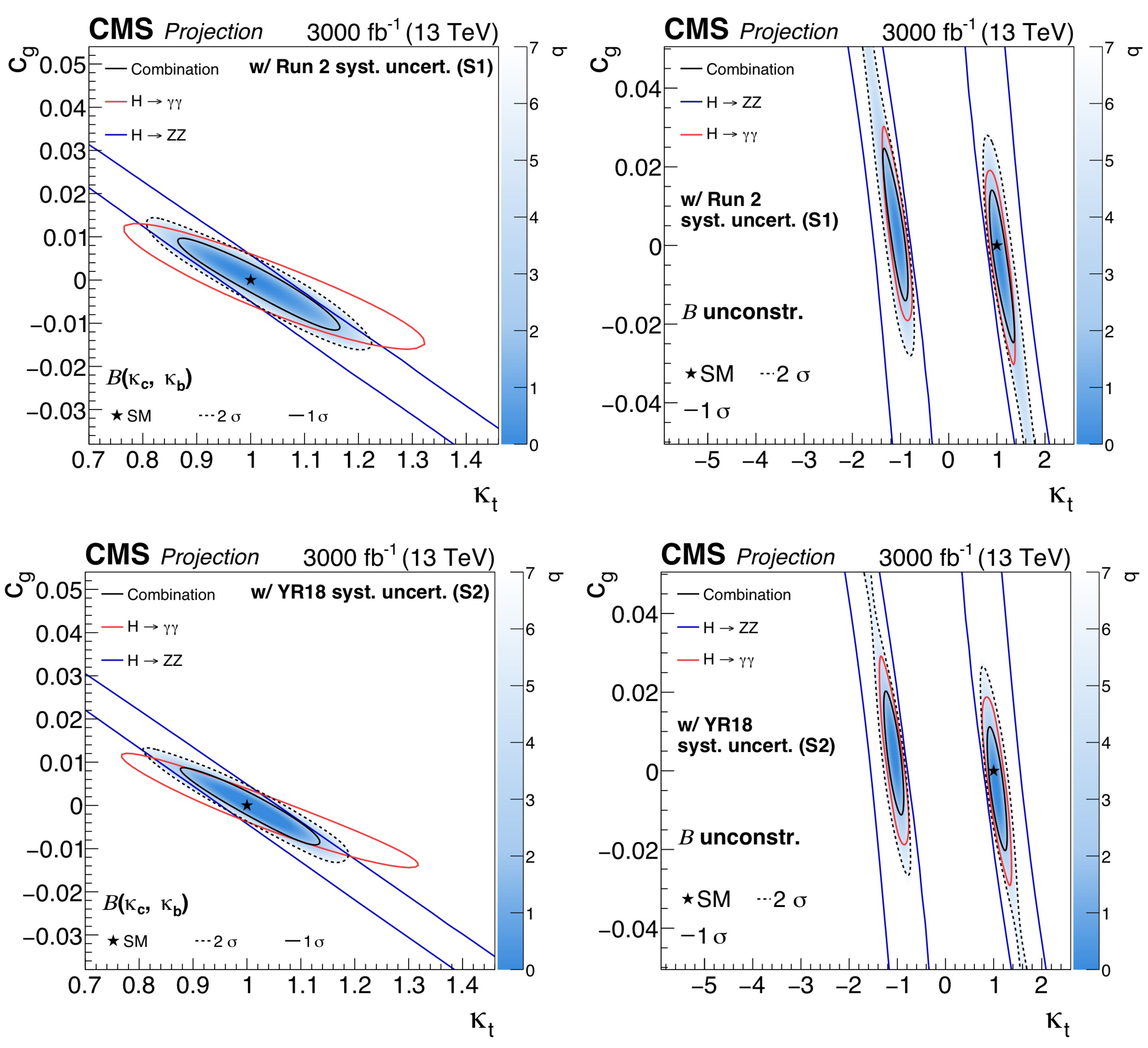
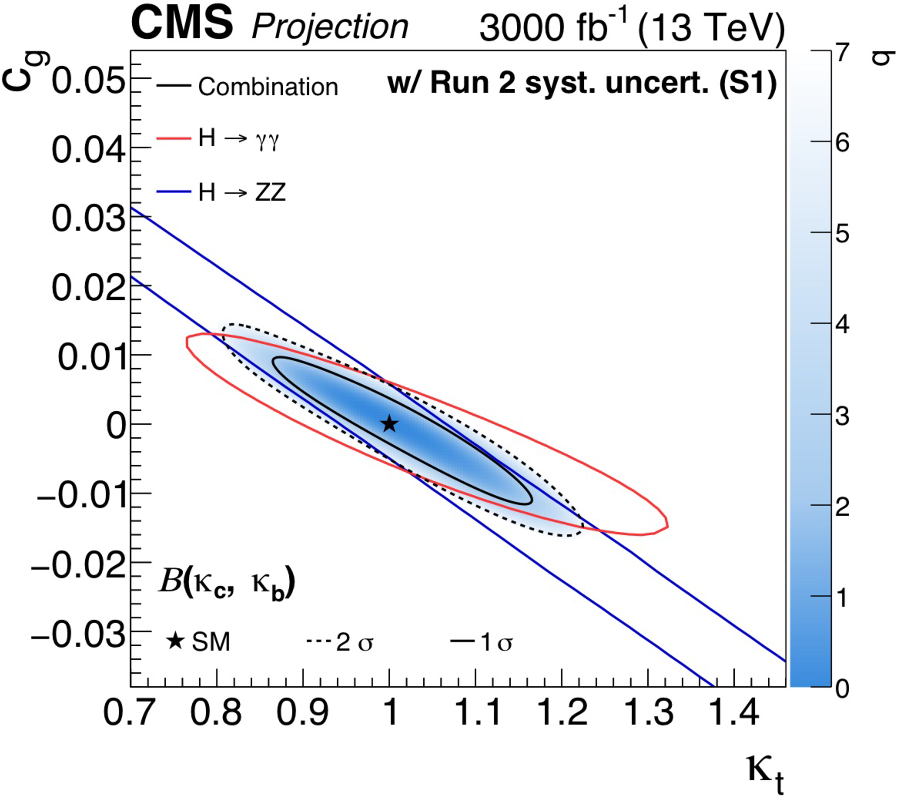
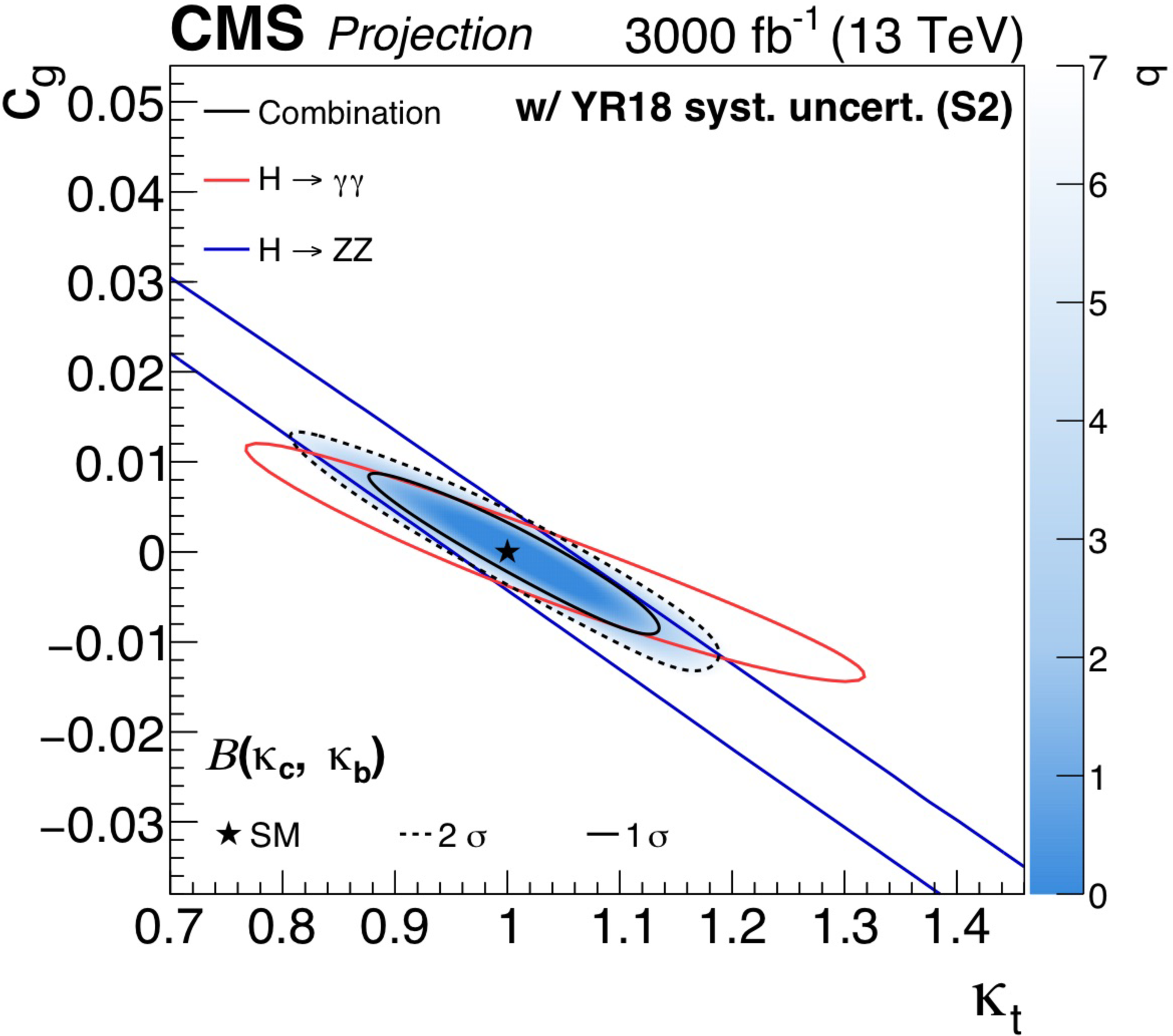
Figure 16:
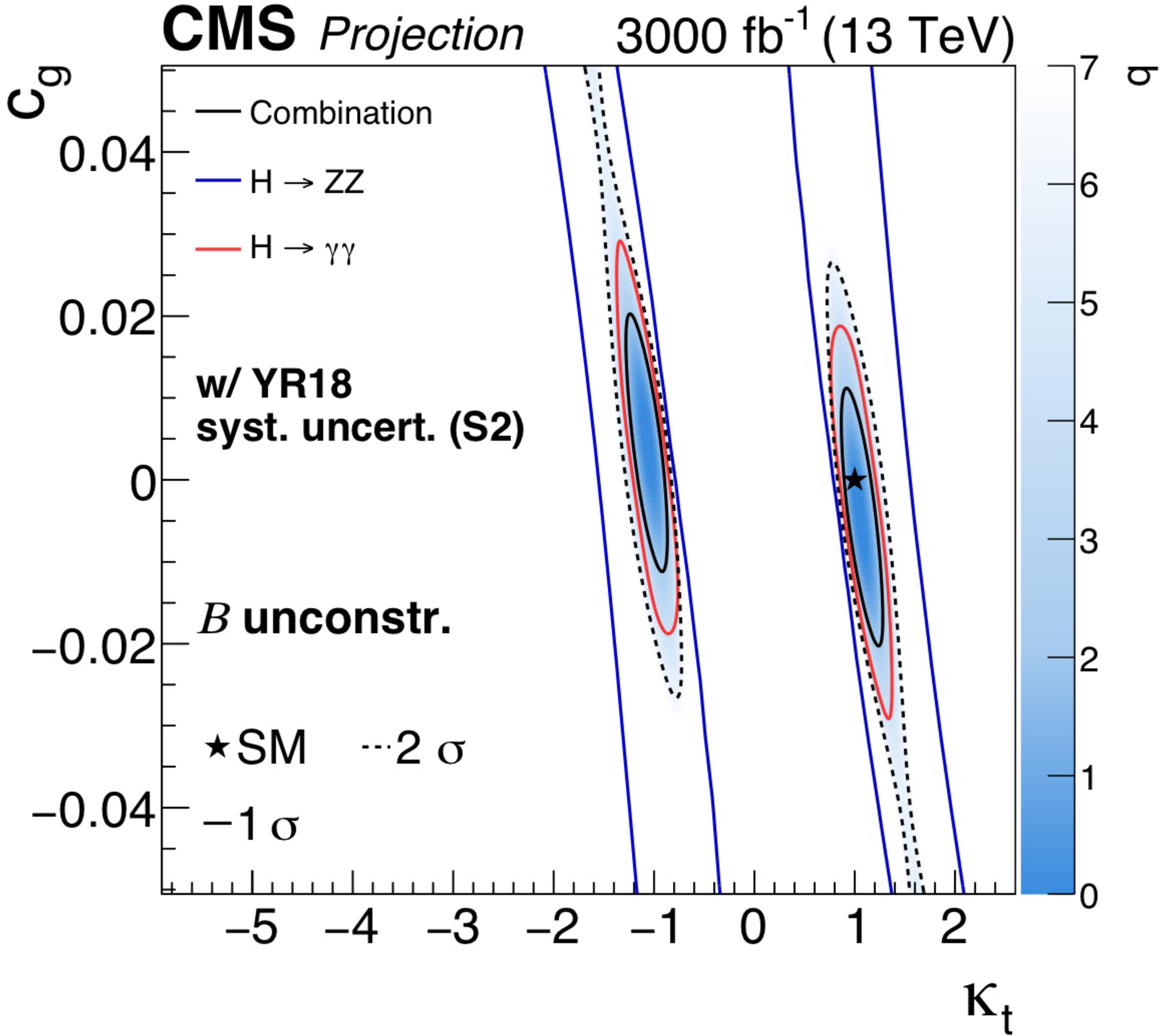
Projected simultaneous fit for $\kappa _\textrm {t}$ and $c_\textrm {g}$, assuming the branching fractions to be determined by the couplings (left) and the branching fractions implemented as nuisance parameters with no prior constraint (right), under S1 (top) and S2 (bottom). The one standard deviation contour is drawn for the combination ($ {{\mathrm {H}} \to {\gamma \gamma}} $, $ {{\mathrm {H}} \to {{\mathrm {Z}} {\mathrm {Z}}}} $, and $ {{\mathrm {H}} \to {\mathrm{b} \mathrm{b}}} $), the $ {{\mathrm {H}} \to {\gamma \gamma}} $ channel, and the $ {{\mathrm {H}} \to {{\mathrm {Z}} {\mathrm {Z}}}} $ channel in black, red, and blue, respectively. For the combination the two standard deviation contour is drawn as a black dashed line, and the shading indicates the negative log-likelihood, with the scale shown on the right hand side of the plots. |
png pdf |
Figure 16-a:
Projected simultaneous fit for $\kappa _\textrm {t}$ and $c_\textrm {g}$, assuming the branching fractions to be determined by the couplings (left) and the branching fractions implemented as nuisance parameters with no prior constraint (right), under S1 (top) and S2 (bottom). The one standard deviation contour is drawn for the combination ($ {{\mathrm {H}} \to {\gamma \gamma}} $, $ {{\mathrm {H}} \to {{\mathrm {Z}} {\mathrm {Z}}}} $, and $ {{\mathrm {H}} \to {\mathrm{b} \mathrm{b}}} $), the $ {{\mathrm {H}} \to {\gamma \gamma}} $ channel, and the $ {{\mathrm {H}} \to {{\mathrm {Z}} {\mathrm {Z}}}} $ channel in black, red, and blue, respectively. For the combination the two standard deviation contour is drawn as a black dashed line, and the shading indicates the negative log-likelihood, with the scale shown on the right hand side of the plots. |

png pdf |
Figure 16-b:
Projected simultaneous fit for $\kappa _\textrm {t}$ and $c_\textrm {g}$, assuming the branching fractions to be determined by the couplings (left) and the branching fractions implemented as nuisance parameters with no prior constraint (right), under S1 (top) and S2 (bottom). The one standard deviation contour is drawn for the combination ($ {{\mathrm {H}} \to {\gamma \gamma}} $, $ {{\mathrm {H}} \to {{\mathrm {Z}} {\mathrm {Z}}}} $, and $ {{\mathrm {H}} \to {\mathrm{b} \mathrm{b}}} $), the $ {{\mathrm {H}} \to {\gamma \gamma}} $ channel, and the $ {{\mathrm {H}} \to {{\mathrm {Z}} {\mathrm {Z}}}} $ channel in black, red, and blue, respectively. For the combination the two standard deviation contour is drawn as a black dashed line, and the shading indicates the negative log-likelihood, with the scale shown on the right hand side of the plots. |
png pdf |
Figure 16-c:
Projected simultaneous fit for $\kappa _\textrm {t}$ and $c_\textrm {g}$, assuming the branching fractions to be determined by the couplings (left) and the branching fractions implemented as nuisance parameters with no prior constraint (right), under S1 (top) and S2 (bottom). The one standard deviation contour is drawn for the combination ($ {{\mathrm {H}} \to {\gamma \gamma}} $, $ {{\mathrm {H}} \to {{\mathrm {Z}} {\mathrm {Z}}}} $, and $ {{\mathrm {H}} \to {\mathrm{b} \mathrm{b}}} $), the $ {{\mathrm {H}} \to {\gamma \gamma}} $ channel, and the $ {{\mathrm {H}} \to {{\mathrm {Z}} {\mathrm {Z}}}} $ channel in black, red, and blue, respectively. For the combination the two standard deviation contour is drawn as a black dashed line, and the shading indicates the negative log-likelihood, with the scale shown on the right hand side of the plots. |
png pdf |
Figure 16-d:
Projected simultaneous fit for $\kappa _\textrm {t}$ and $c_\textrm {g}$, assuming the branching fractions to be determined by the couplings (left) and the branching fractions implemented as nuisance parameters with no prior constraint (right), under S1 (top) and S2 (bottom). The one standard deviation contour is drawn for the combination ($ {{\mathrm {H}} \to {\gamma \gamma}} $, $ {{\mathrm {H}} \to {{\mathrm {Z}} {\mathrm {Z}}}} $, and $ {{\mathrm {H}} \to {\mathrm{b} \mathrm{b}}} $), the $ {{\mathrm {H}} \to {\gamma \gamma}} $ channel, and the $ {{\mathrm {H}} \to {{\mathrm {Z}} {\mathrm {Z}}}} $ channel in black, red, and blue, respectively. For the combination the two standard deviation contour is drawn as a black dashed line, and the shading indicates the negative log-likelihood, with the scale shown on the right hand side of the plots. |
png pdf |
Figure 17:
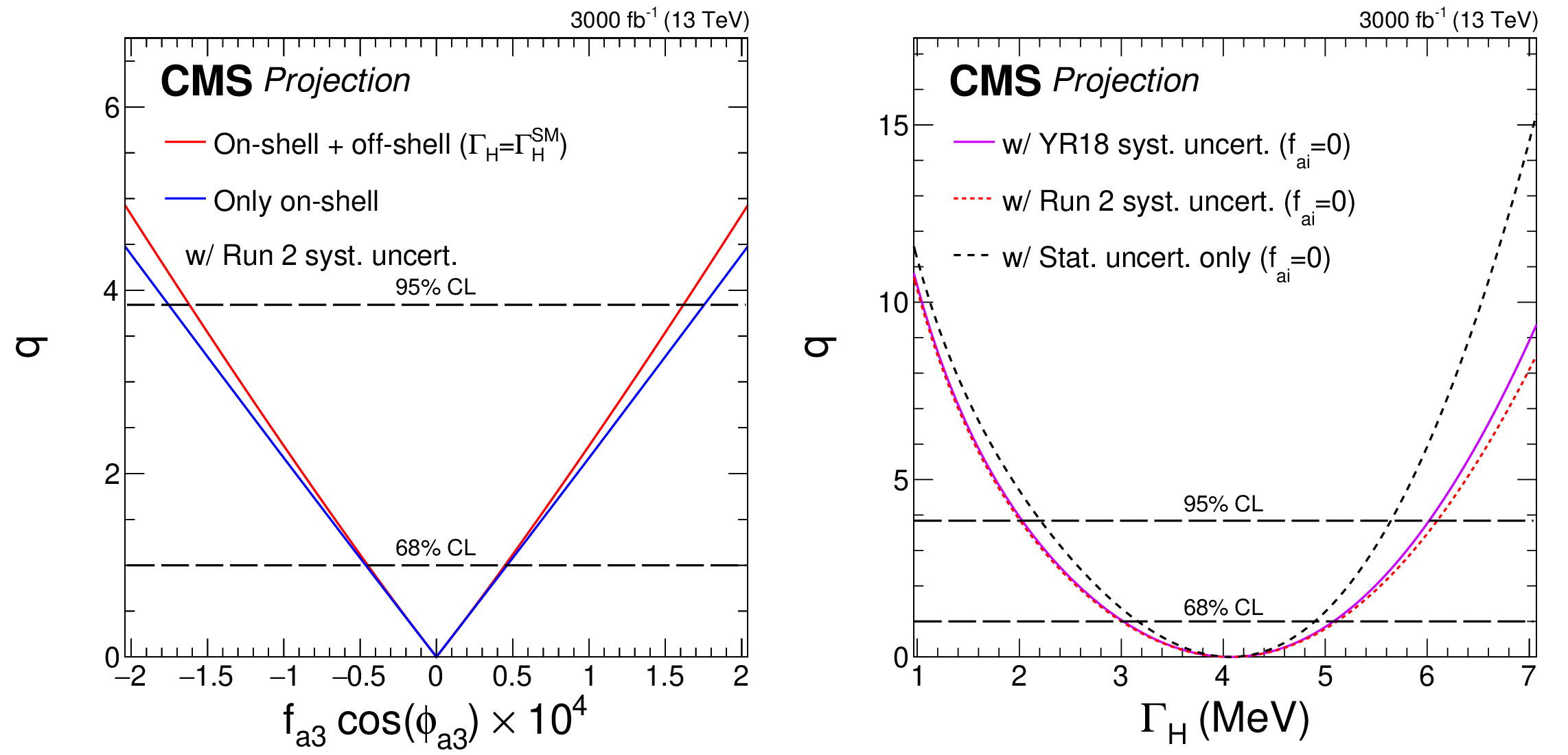
Likelihood scans for projections on ${{f_{a 3}} {\cos\left ({\phi _{a 3}} \right)}}$ (left) and ${\Gamma _ {\mathrm {H}}}$ (right) at 3000 fb$^{-1}$. On the left plot, the scans are shown using either the combination of on-shell and off-shell events (red) or only on-shell events (blue). The dashed lines represent the effect of removing all systematic uncertainties. In the right plot, scenarios S2 (solid magenta) and S1 (dotted red) are compared to the case where all systematic uncertainties (dashed black) are removed. The dashed horizontal lines indicate the 68% and 95% CLs. The ${{f_{a 3}} {\cos\left ({\phi _{a 3}} \right)}}$ scans assume $ {\Gamma _ {\mathrm {H}}} = {\Gamma _ {\mathrm {H}} ^{\mathrm {SM}}} $, and the ${\Gamma _ {\mathrm {H}}}$ scans assume $ {f_{a i}} =$ 0. |

png pdf |
Figure 17-a:
Likelihood scans for projections on ${{f_{a 3}} {\cos\left ({\phi _{a 3}} \right)}}$ (left) and ${\Gamma _ {\mathrm {H}}}$ (right) at 3000 fb$^{-1}$. On the left plot, the scans are shown using either the combination of on-shell and off-shell events (red) or only on-shell events (blue). The dashed lines represent the effect of removing all systematic uncertainties. In the right plot, scenarios S2 (solid magenta) and S1 (dotted red) are compared to the case where all systematic uncertainties (dashed black) are removed. The dashed horizontal lines indicate the 68% and 95% CLs. The ${{f_{a 3}} {\cos\left ({\phi _{a 3}} \right)}}$ scans assume $ {\Gamma _ {\mathrm {H}}} = {\Gamma _ {\mathrm {H}} ^{\mathrm {SM}}} $, and the ${\Gamma _ {\mathrm {H}}}$ scans assume $ {f_{a i}} =$ 0. |

png pdf |
Figure 17-b:
Likelihood scans for projections on ${{f_{a 3}} {\cos\left ({\phi _{a 3}} \right)}}$ (left) and ${\Gamma _ {\mathrm {H}}}$ (right) at 3000 fb$^{-1}$. On the left plot, the scans are shown using either the combination of on-shell and off-shell events (red) or only on-shell events (blue). The dashed lines represent the effect of removing all systematic uncertainties. In the right plot, scenarios S2 (solid magenta) and S1 (dotted red) are compared to the case where all systematic uncertainties (dashed black) are removed. The dashed horizontal lines indicate the 68% and 95% CLs. The ${{f_{a 3}} {\cos\left ({\phi _{a 3}} \right)}}$ scans assume $ {\Gamma _ {\mathrm {H}}} = {\Gamma _ {\mathrm {H}} ^{\mathrm {SM}}} $, and the ${\Gamma _ {\mathrm {H}}}$ scans assume $ {f_{a i}} =$ 0. |
png pdf |
Figure 18:
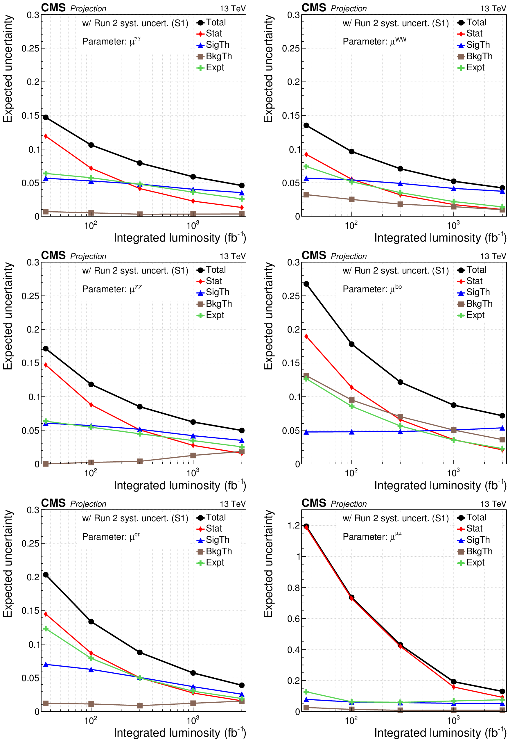
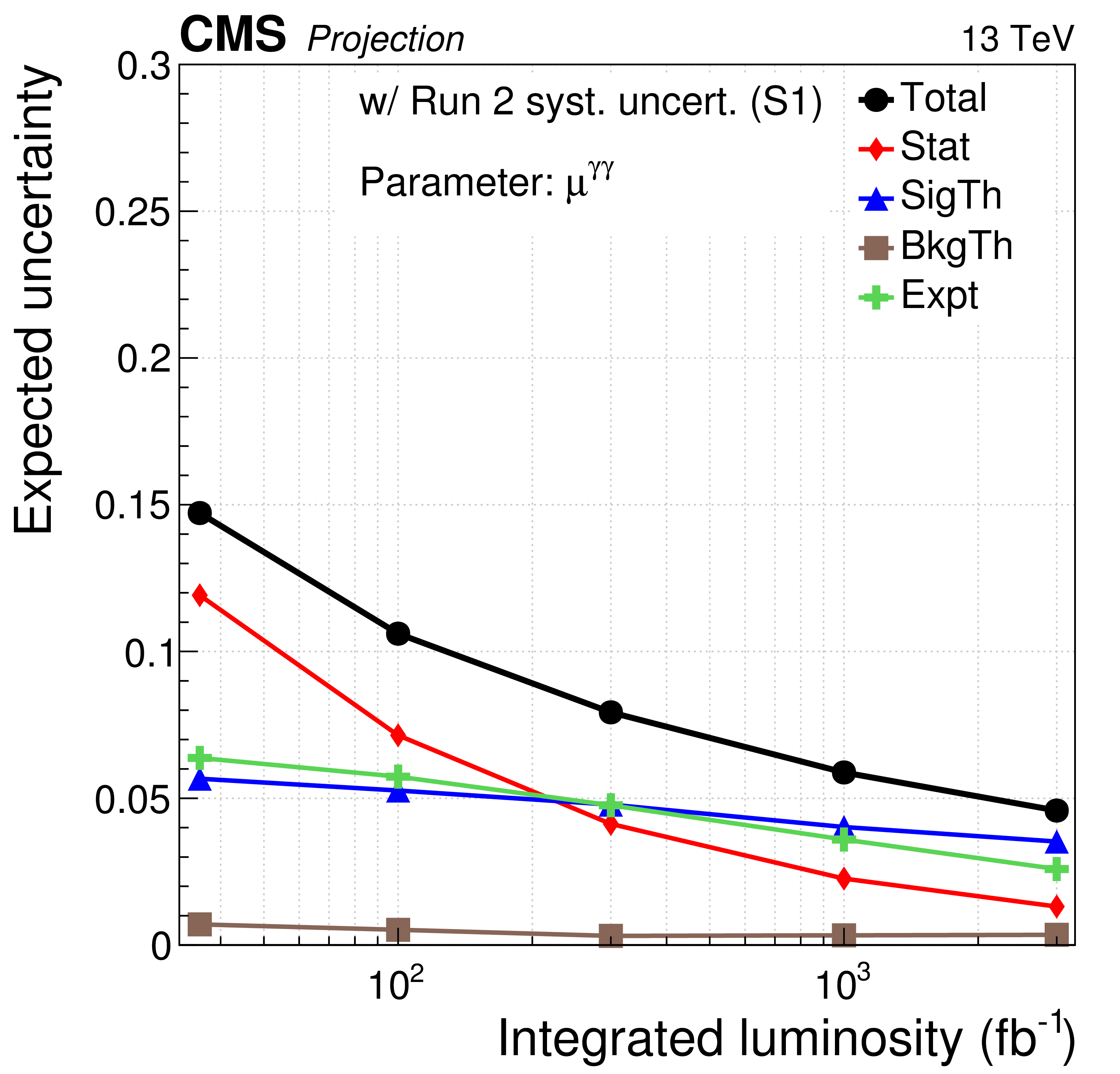
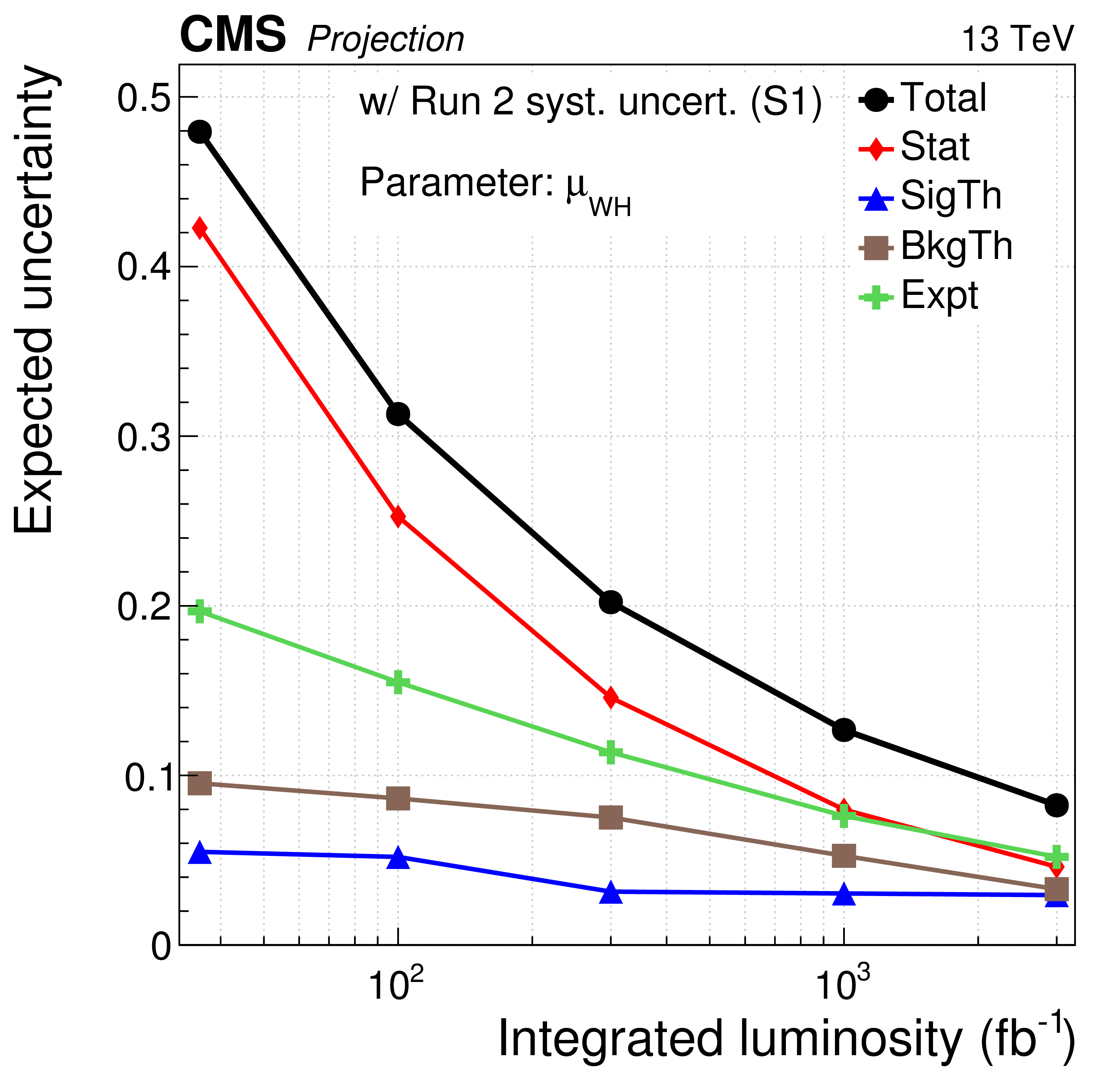
Evolution of the uncertainty contribution with integrated luminosity for the per-decay signal strength parameters in S1 (with Run 2 systematic uncertainties [30]). |
png pdf |
Figure 18-a:
Evolution of the uncertainty contribution with integrated luminosity for the per-decay signal strength parameters in S1 (with Run 2 systematic uncertainties [30]). |

png pdf |
Figure 18-b:
Evolution of the uncertainty contribution with integrated luminosity for the per-decay signal strength parameters in S1 (with Run 2 systematic uncertainties [30]). |
png pdf |
Figure 18-c:
Evolution of the uncertainty contribution with integrated luminosity for the per-decay signal strength parameters in S1 (with Run 2 systematic uncertainties [30]). |

png pdf |
Figure 18-d:
Evolution of the uncertainty contribution with integrated luminosity for the per-decay signal strength parameters in S1 (with Run 2 systematic uncertainties [30]). |

png pdf |
Figure 18-e:
Evolution of the uncertainty contribution with integrated luminosity for the per-decay signal strength parameters in S1 (with Run 2 systematic uncertainties [30]). |

png pdf |
Figure 18-f:
Evolution of the uncertainty contribution with integrated luminosity for the per-decay signal strength parameters in S1 (with Run 2 systematic uncertainties [30]). |
png pdf |
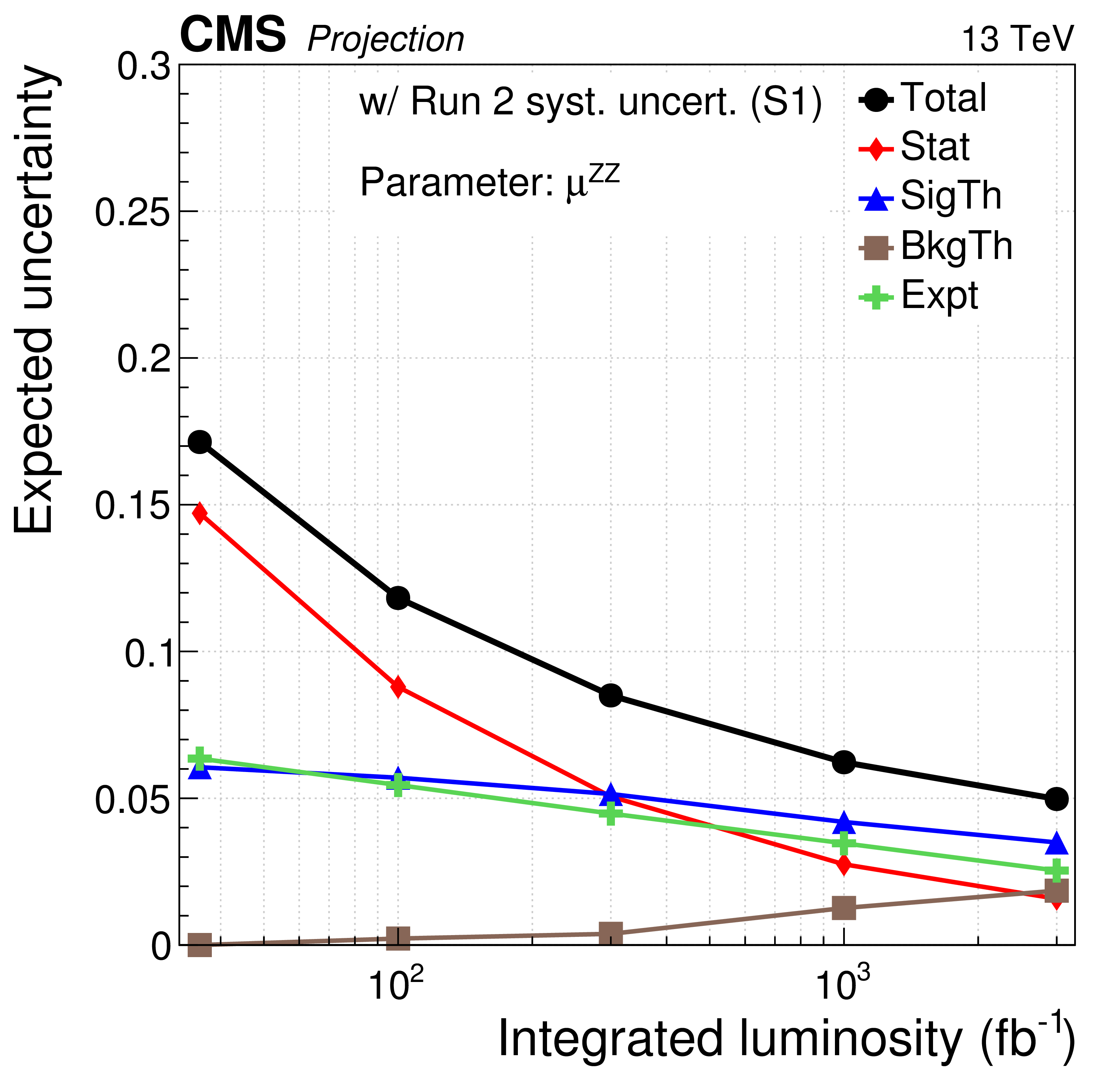
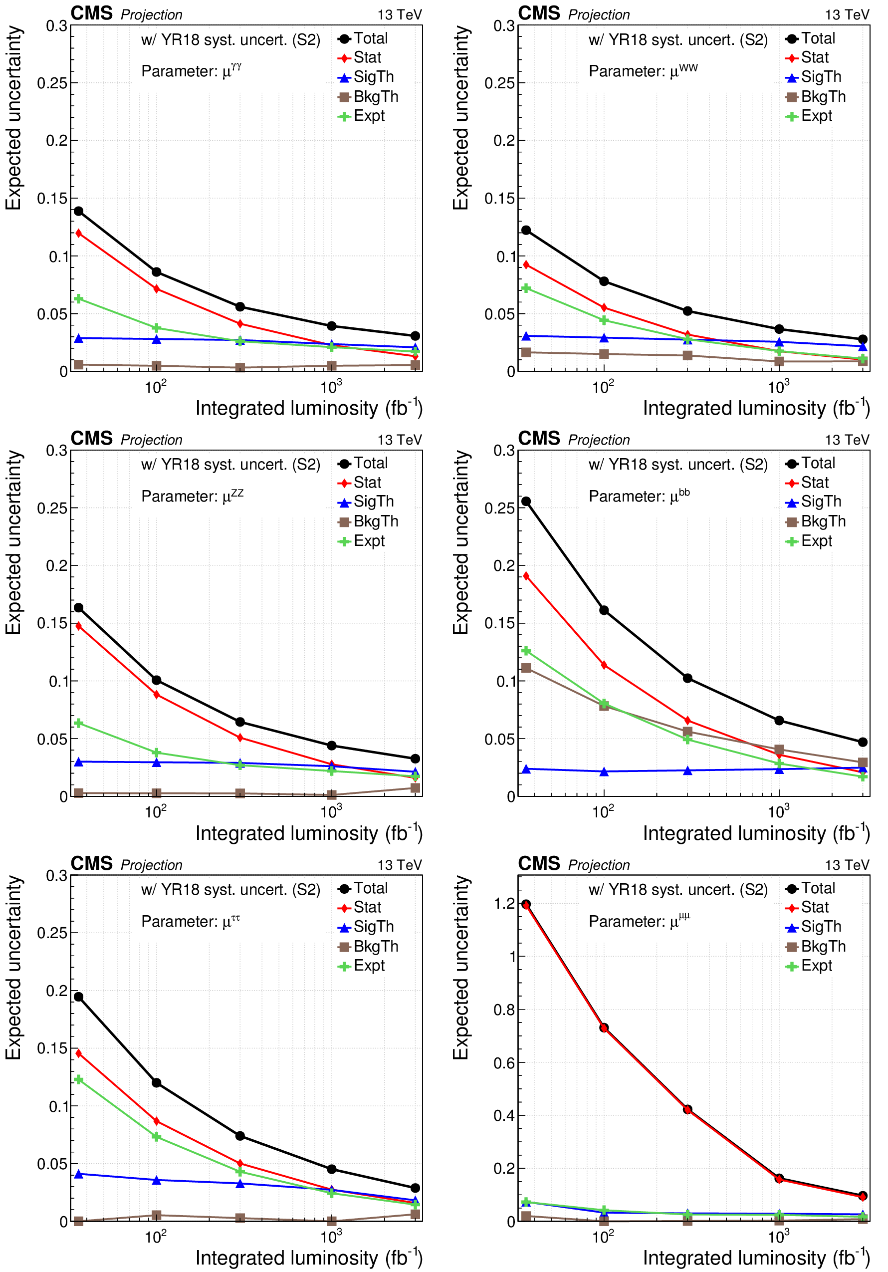
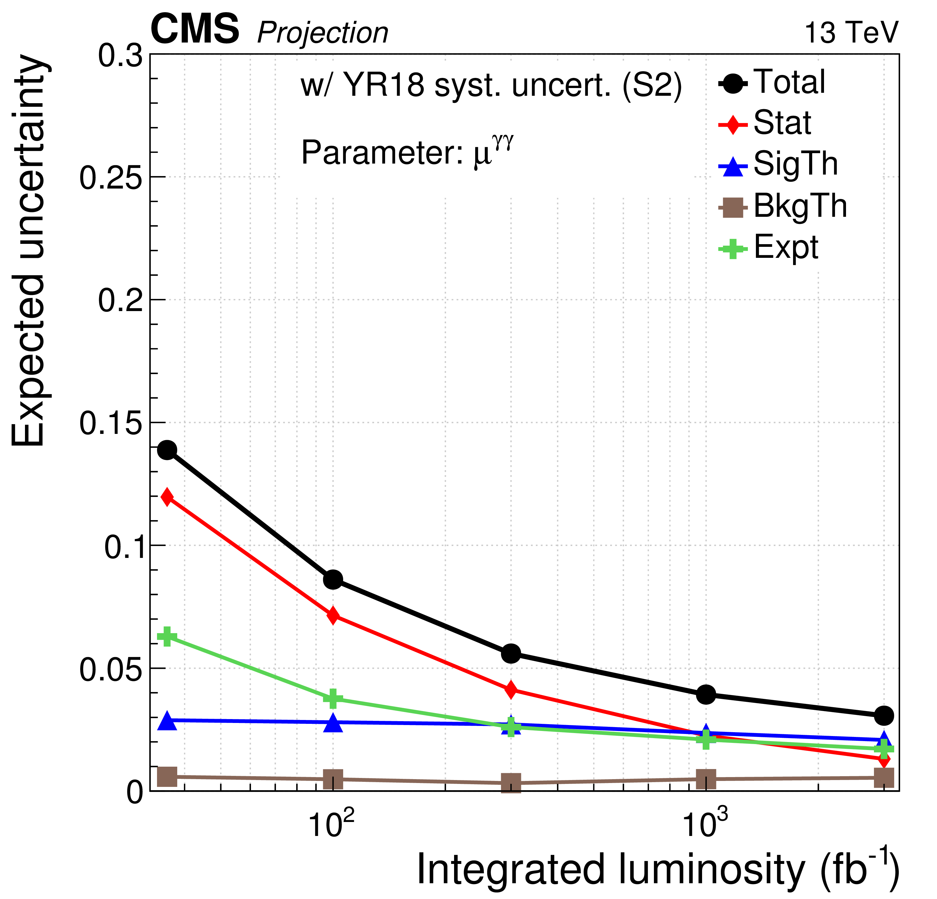
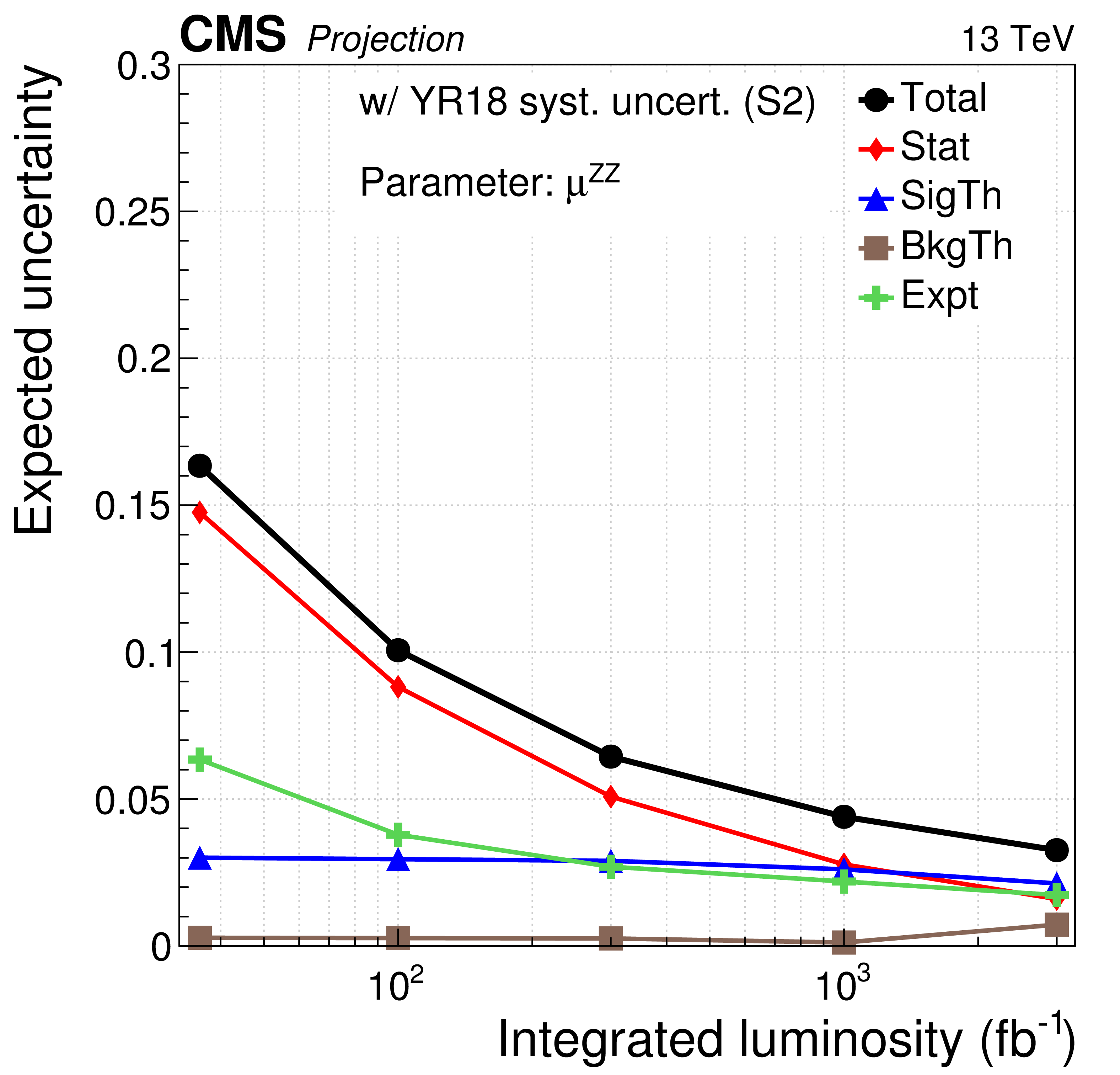
Figure 19:
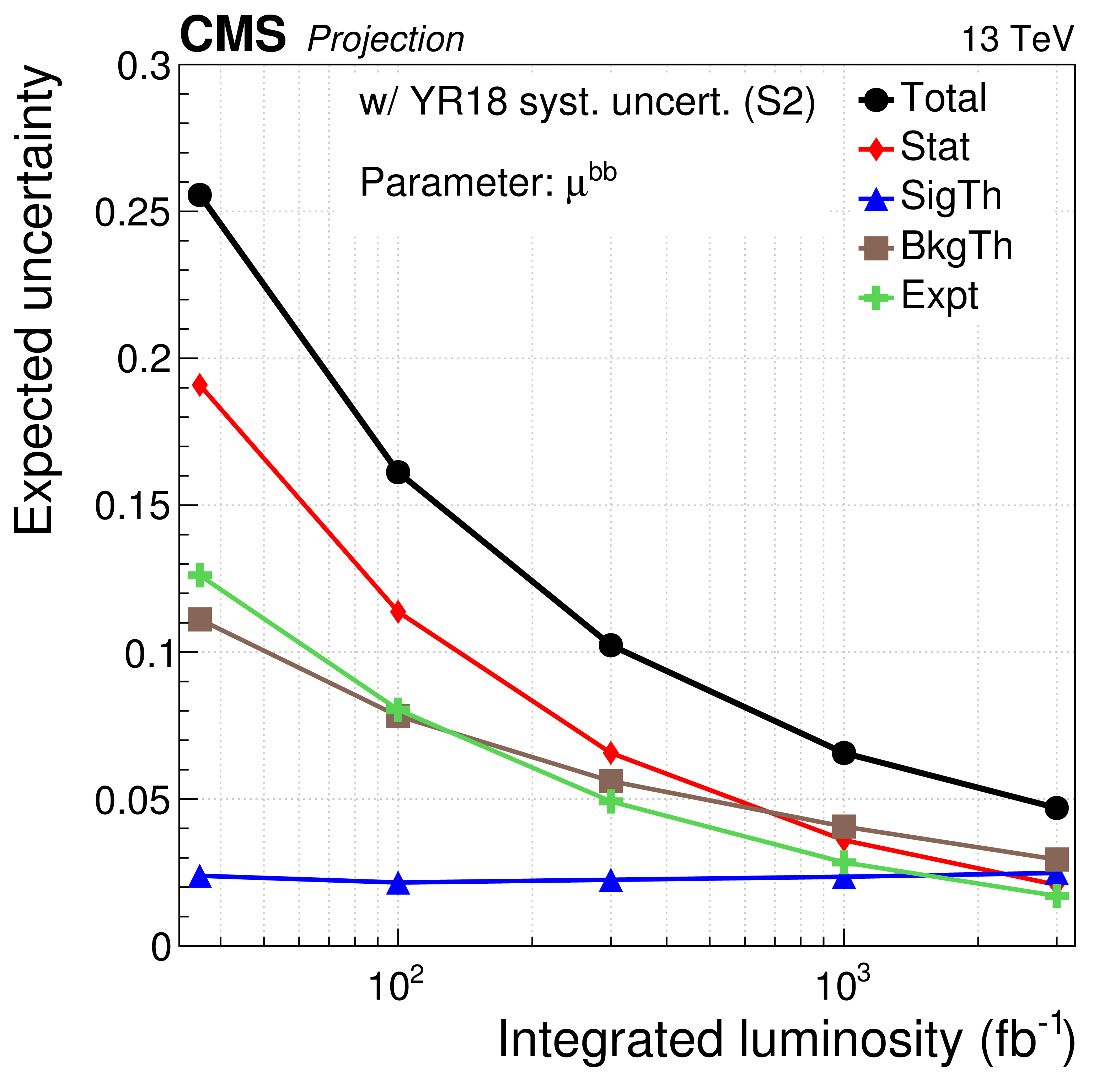
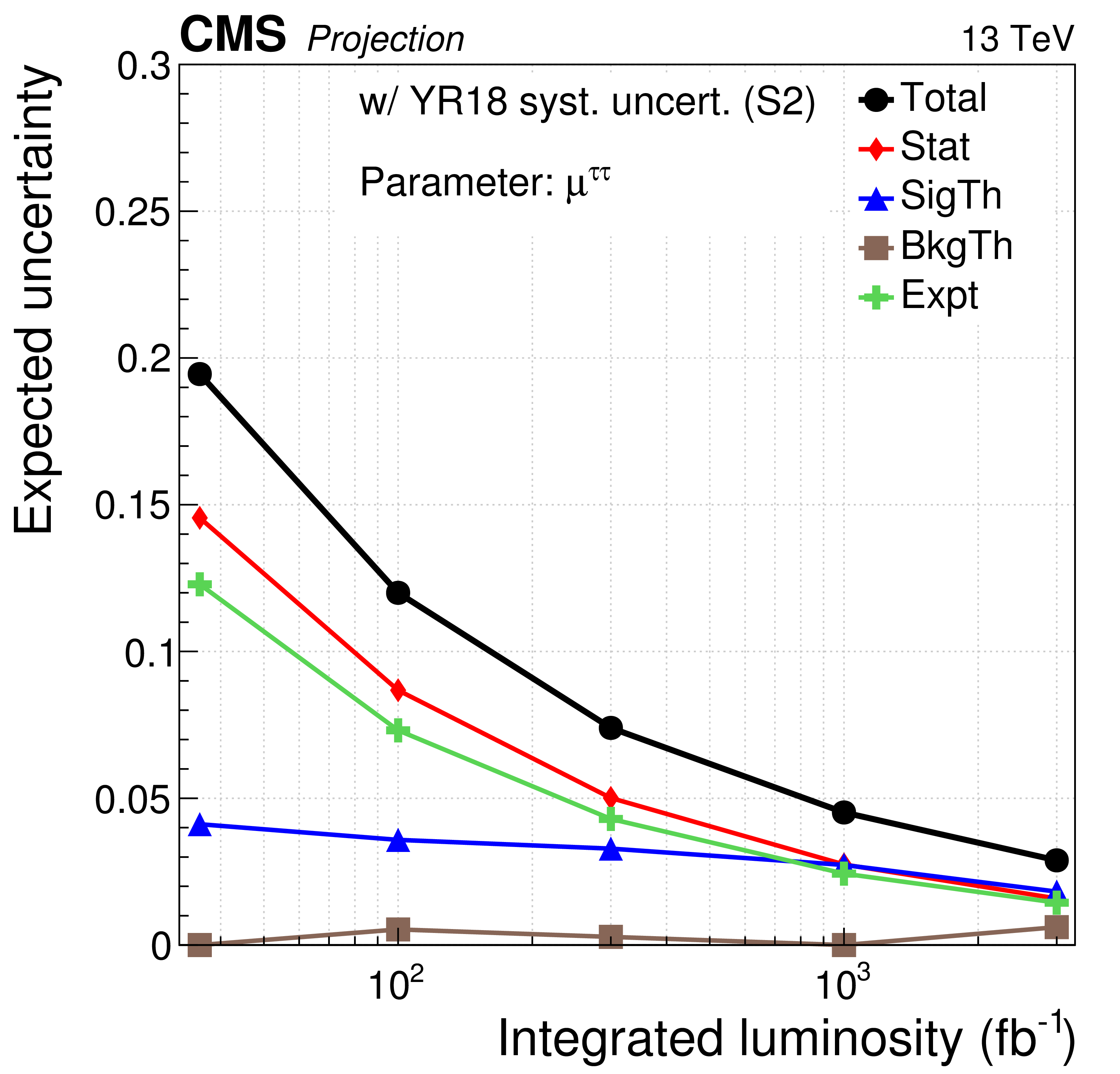
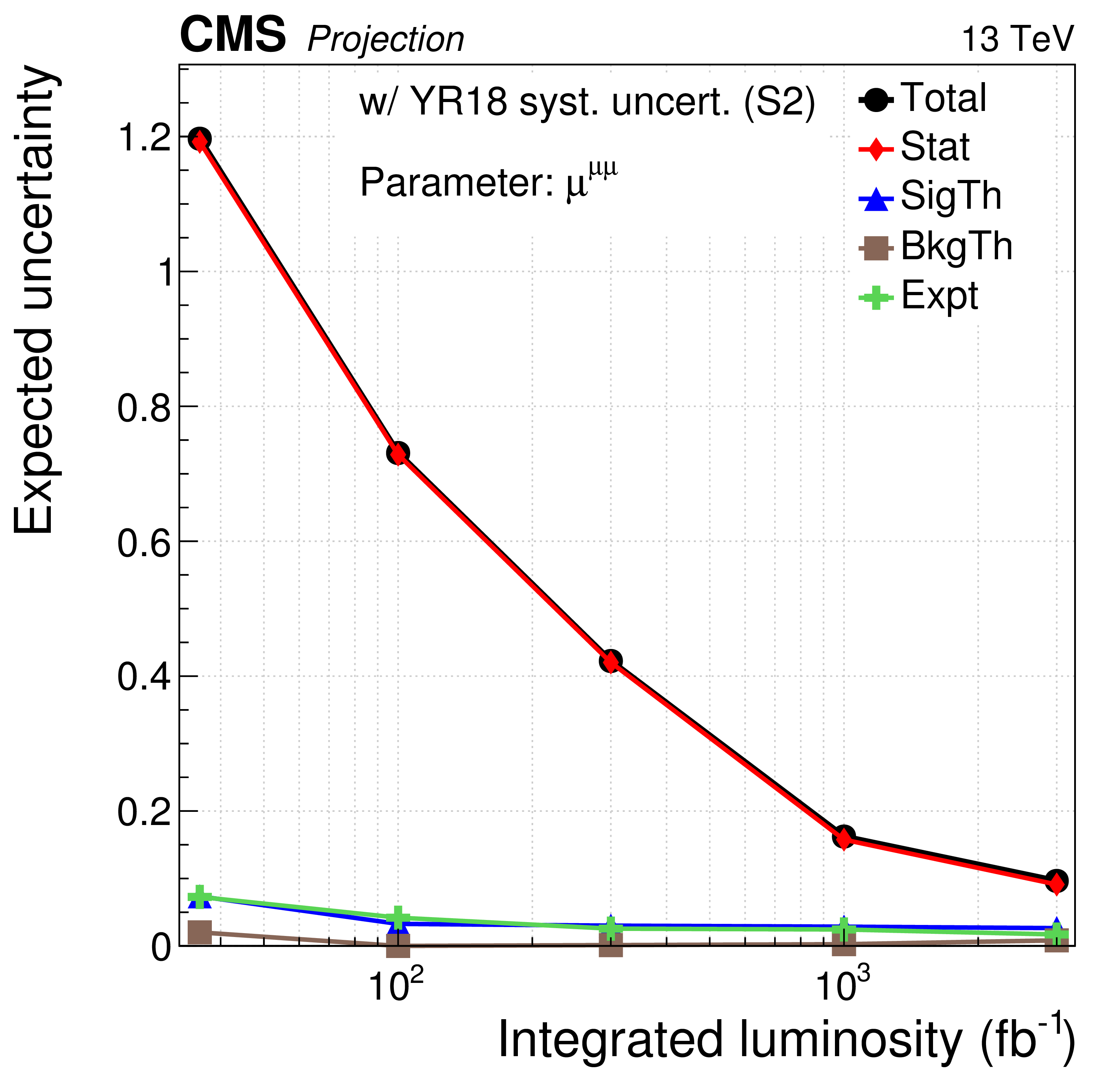
Evolution of the uncertainty contribution with integrated luminosity for the per-decay signal strength parameters in S2 (with YR18 systematic uncertainties). |
png pdf |
Figure 19-a:
Evolution of the uncertainty contribution with integrated luminosity for the per-decay signal strength parameters in S2 (with YR18 systematic uncertainties). |

png pdf |
Figure 19-b:
Evolution of the uncertainty contribution with integrated luminosity for the per-decay signal strength parameters in S2 (with YR18 systematic uncertainties). |
png pdf |
Figure 19-c:
Evolution of the uncertainty contribution with integrated luminosity for the per-decay signal strength parameters in S2 (with YR18 systematic uncertainties). |
png pdf |
Figure 19-d:
Evolution of the uncertainty contribution with integrated luminosity for the per-decay signal strength parameters in S2 (with YR18 systematic uncertainties). |
png pdf |
Figure 19-e:
Evolution of the uncertainty contribution with integrated luminosity for the per-decay signal strength parameters in S2 (with YR18 systematic uncertainties). |
png pdf |
Figure 19-f:
Evolution of the uncertainty contribution with integrated luminosity for the per-decay signal strength parameters in S2 (with YR18 systematic uncertainties). |

png pdf |
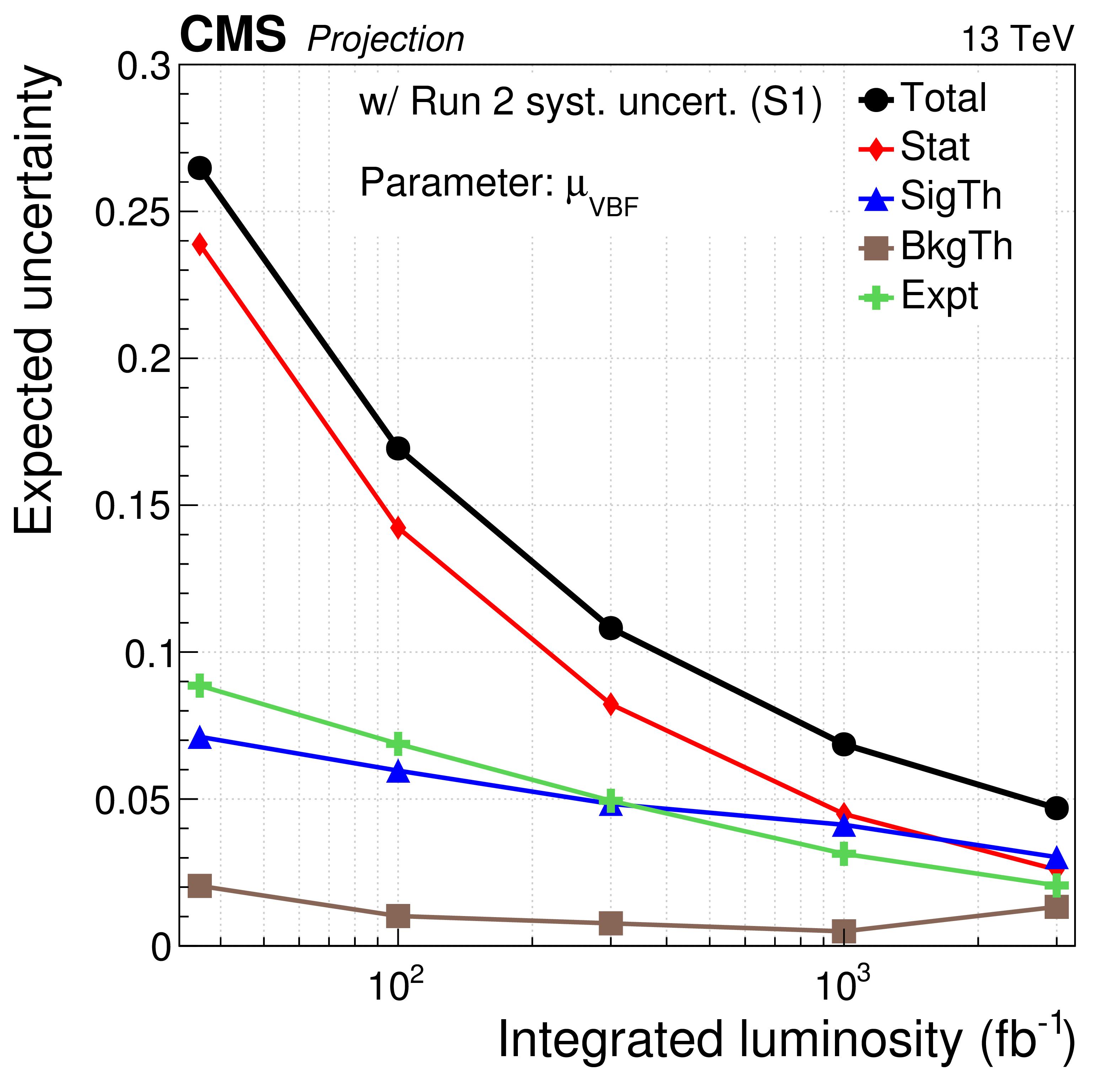
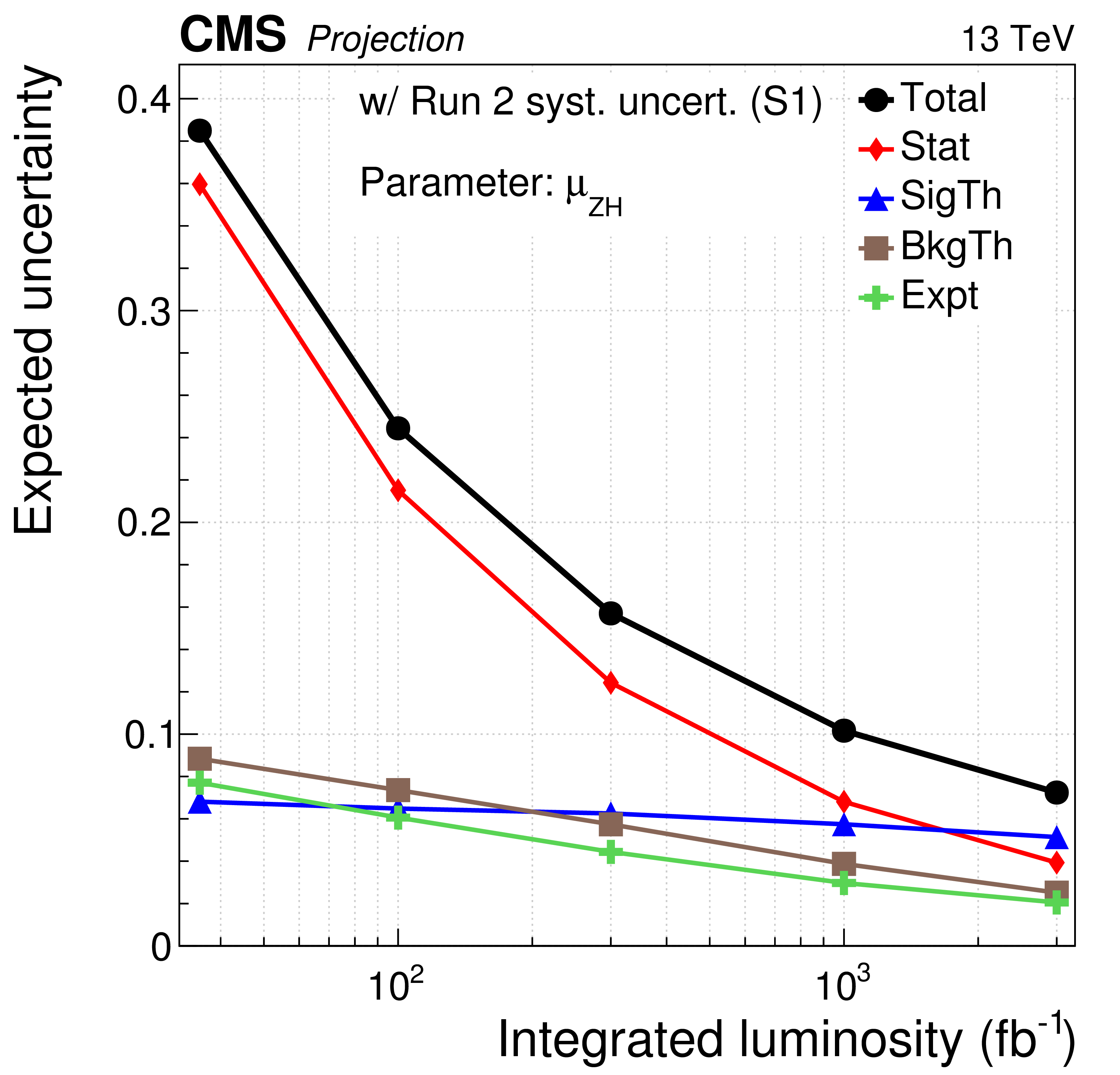
Figure 20:
Evolution of the uncertainty contribution with integrated luminosity for the per-production signal strength parameters in S1 (with Run 2 systematic uncertainties [30]). |

png pdf |
Figure 20-a:
Evolution of the uncertainty contribution with integrated luminosity for the per-production signal strength parameters in S1 (with Run 2 systematic uncertainties [30]). |
png pdf |
Figure 20-b:
Evolution of the uncertainty contribution with integrated luminosity for the per-production signal strength parameters in S1 (with Run 2 systematic uncertainties [30]). |
png pdf |
Figure 20-c:
Evolution of the uncertainty contribution with integrated luminosity for the per-production signal strength parameters in S1 (with Run 2 systematic uncertainties [30]). |
png pdf |
Figure 20-d:
Evolution of the uncertainty contribution with integrated luminosity for the per-production signal strength parameters in S1 (with Run 2 systematic uncertainties [30]). |

png pdf |
Figure 20-e:
Evolution of the uncertainty contribution with integrated luminosity for the per-production signal strength parameters in S1 (with Run 2 systematic uncertainties [30]). |
png pdf |
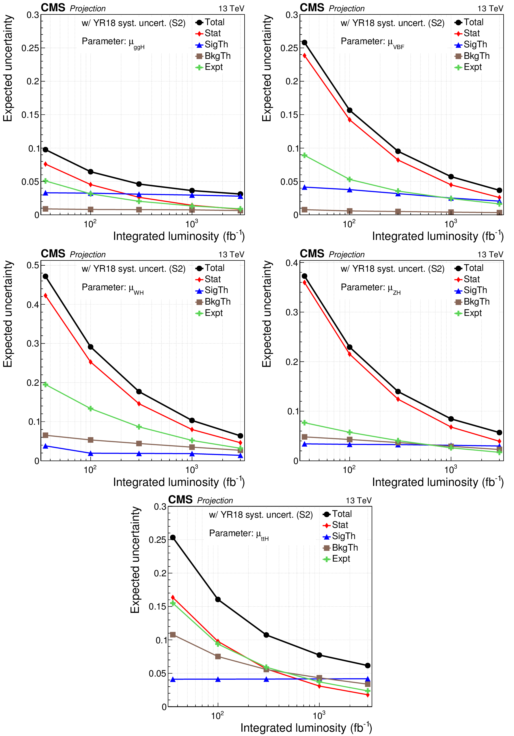
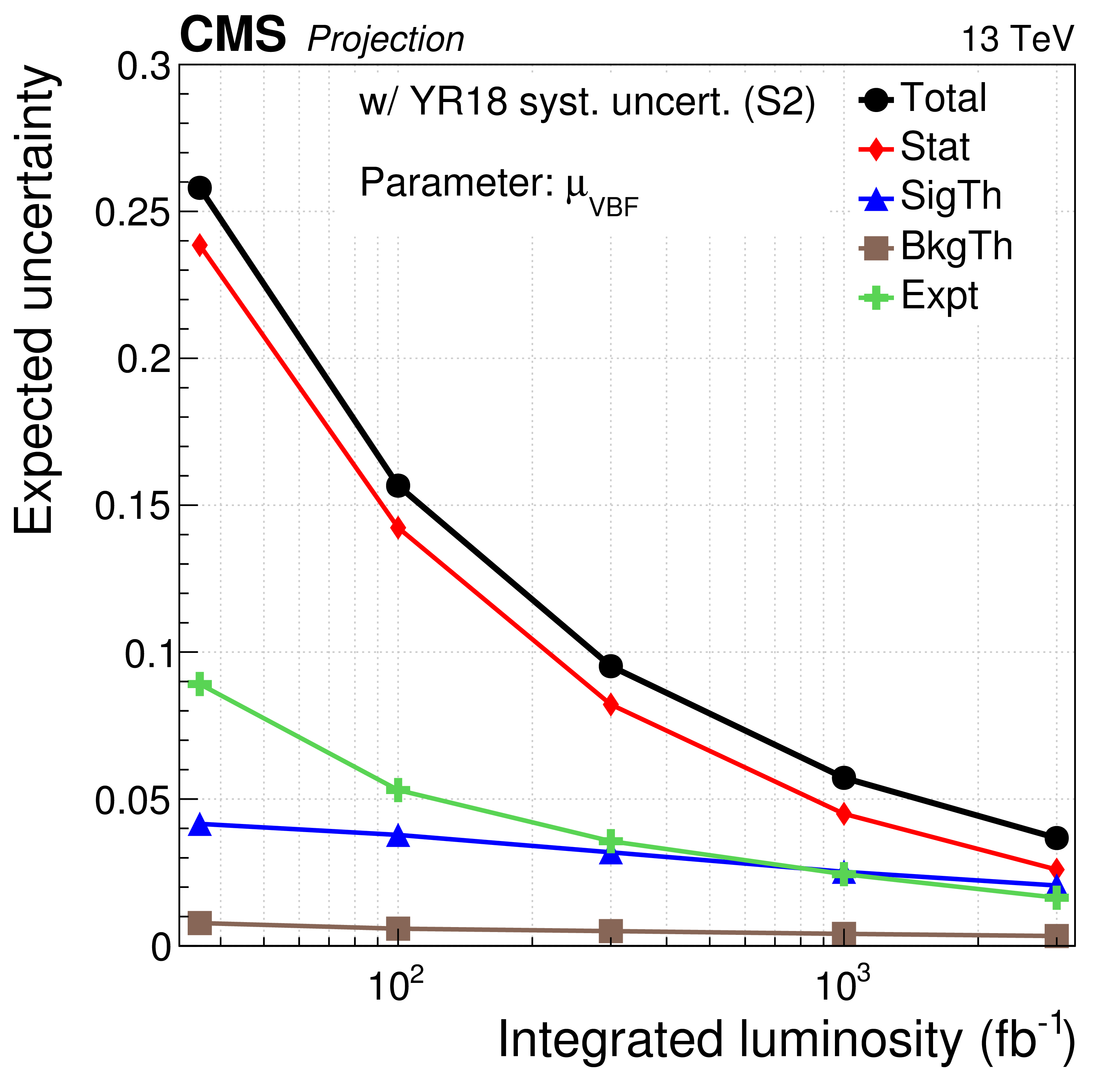
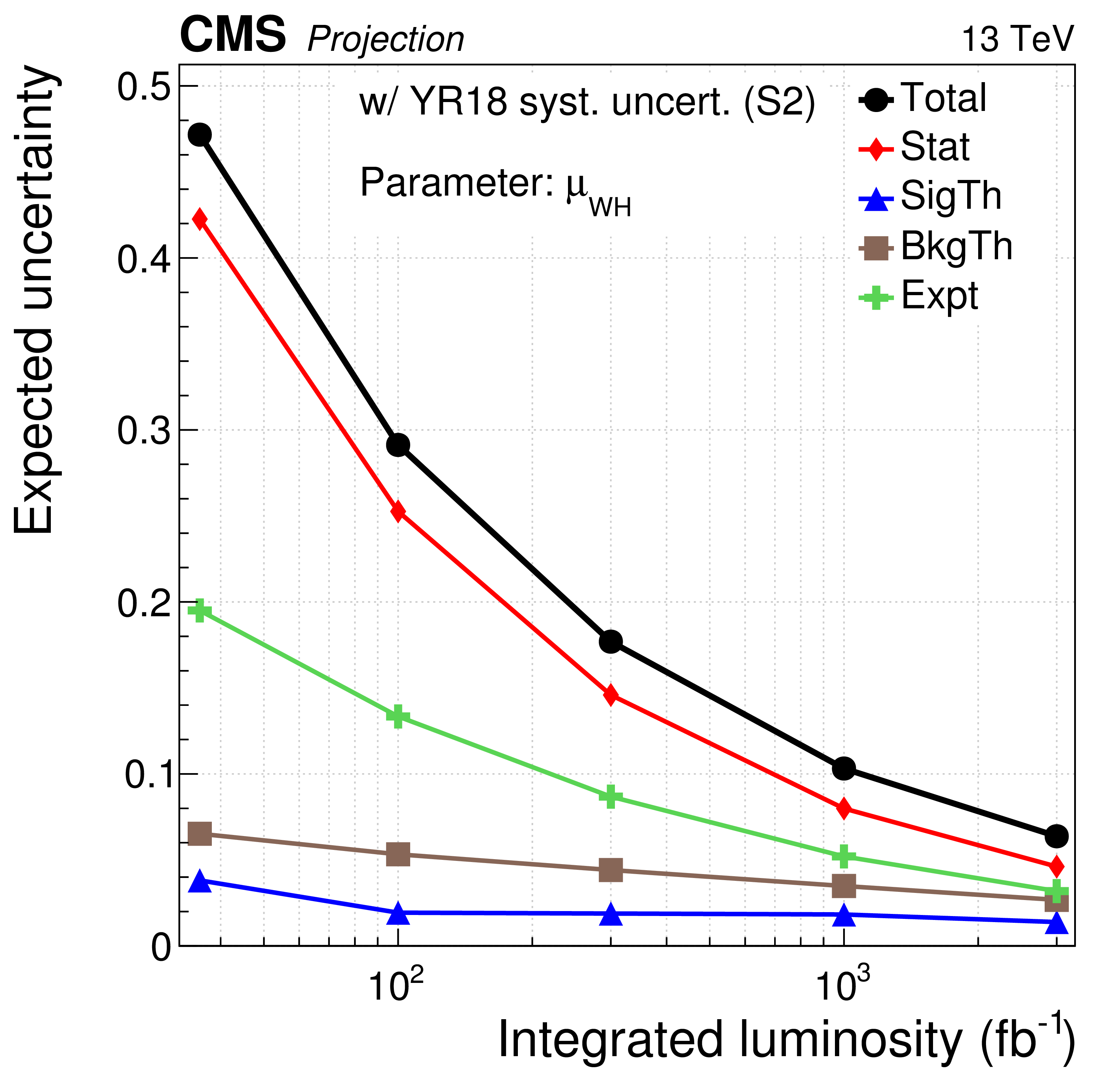
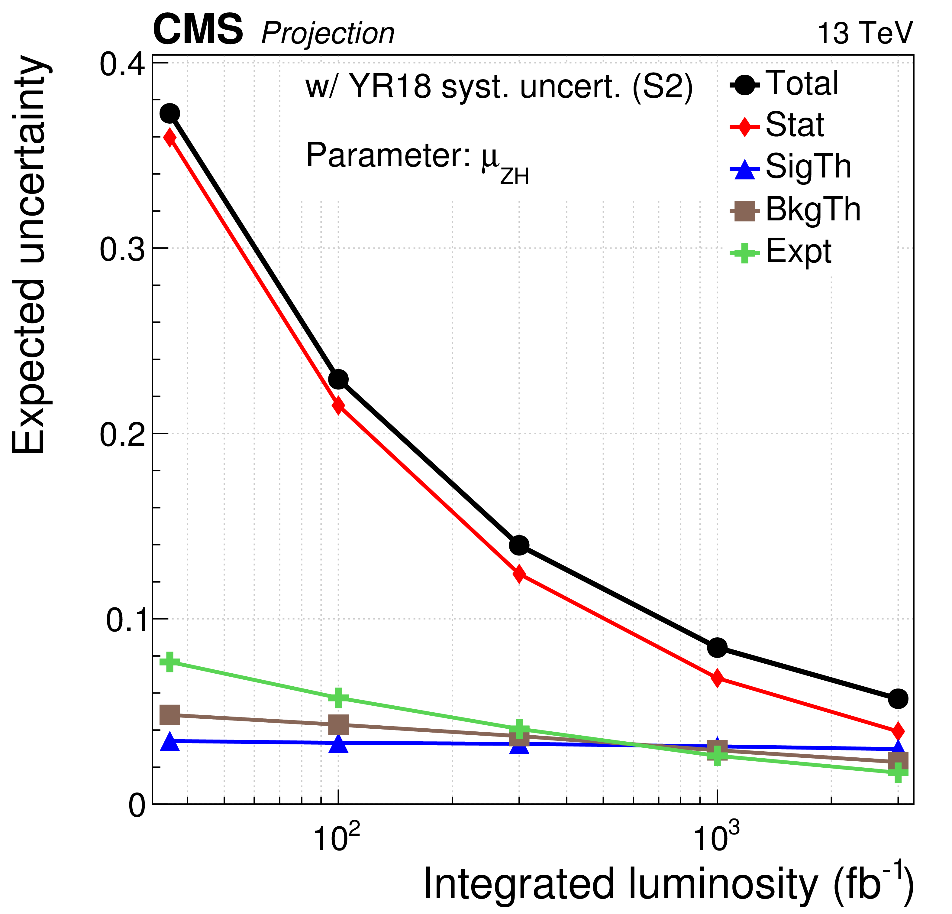
Figure 21:
Evolution of the uncertainty contribution with integrated luminosity for the per-production signal strength parameters in S2 (with YR18 systematic uncertainties). |

png pdf |
Figure 21-a:
Evolution of the uncertainty contribution with integrated luminosity for the per-production signal strength parameters in S2 (with YR18 systematic uncertainties). |
png pdf |
Figure 21-b:
Evolution of the uncertainty contribution with integrated luminosity for the per-production signal strength parameters in S2 (with YR18 systematic uncertainties). |
png pdf |
Figure 21-c:
Evolution of the uncertainty contribution with integrated luminosity for the per-production signal strength parameters in S2 (with YR18 systematic uncertainties). |
png pdf |
Figure 21-d:
Evolution of the uncertainty contribution with integrated luminosity for the per-production signal strength parameters in S2 (with YR18 systematic uncertainties). |

png pdf |
Figure 21-e:
Evolution of the uncertainty contribution with integrated luminosity for the per-production signal strength parameters in S2 (with YR18 systematic uncertainties). |
png pdf |
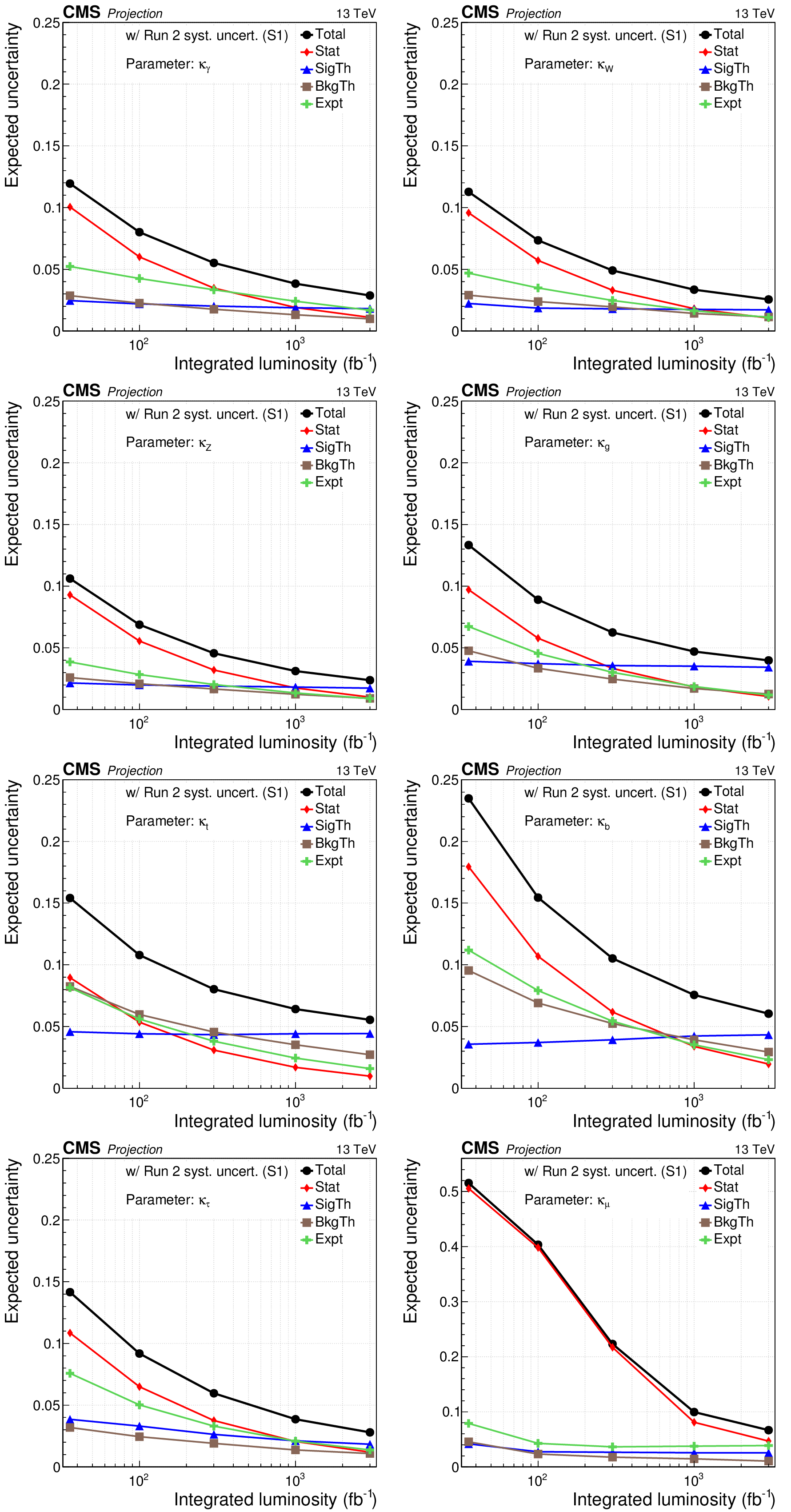
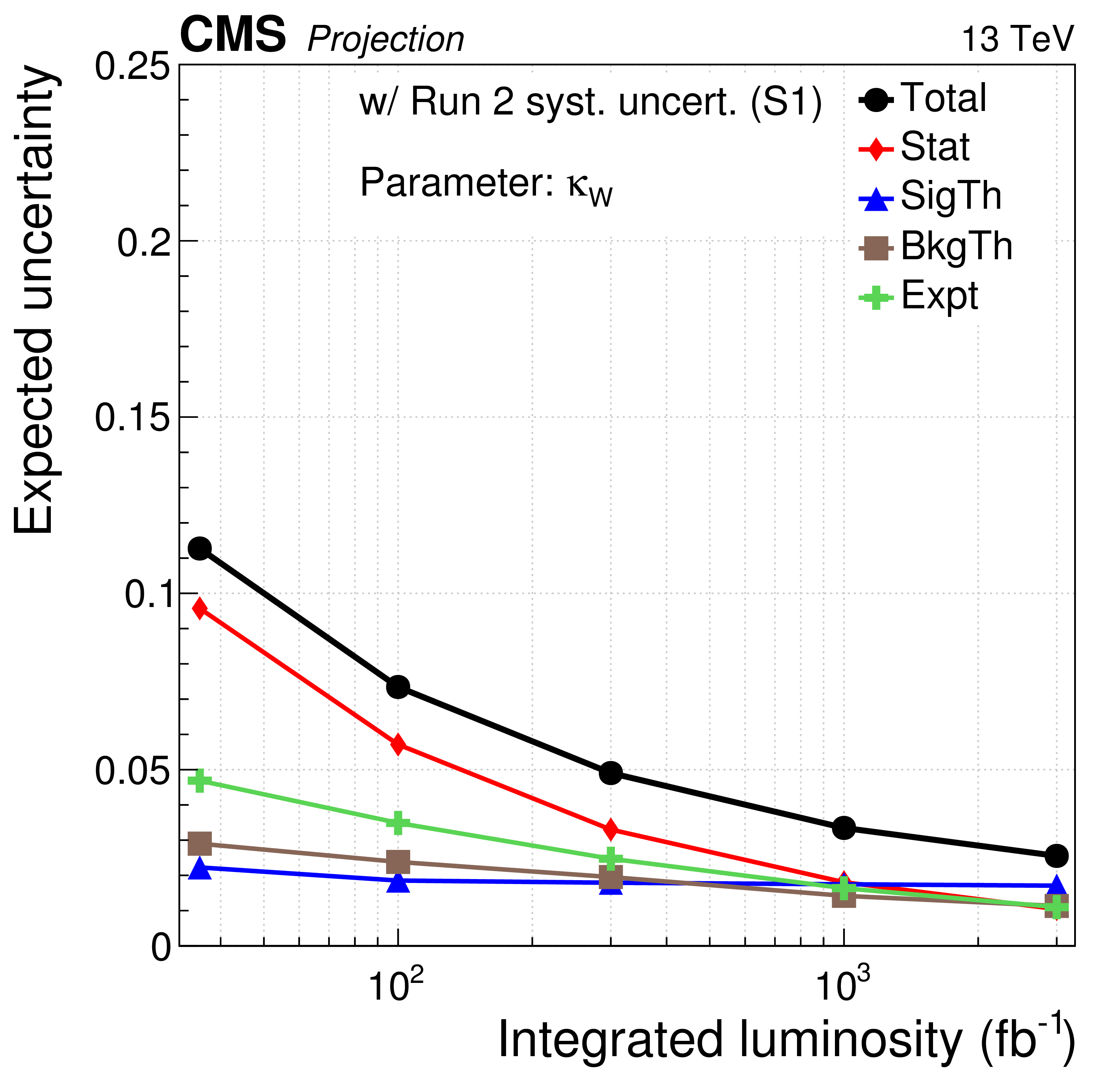
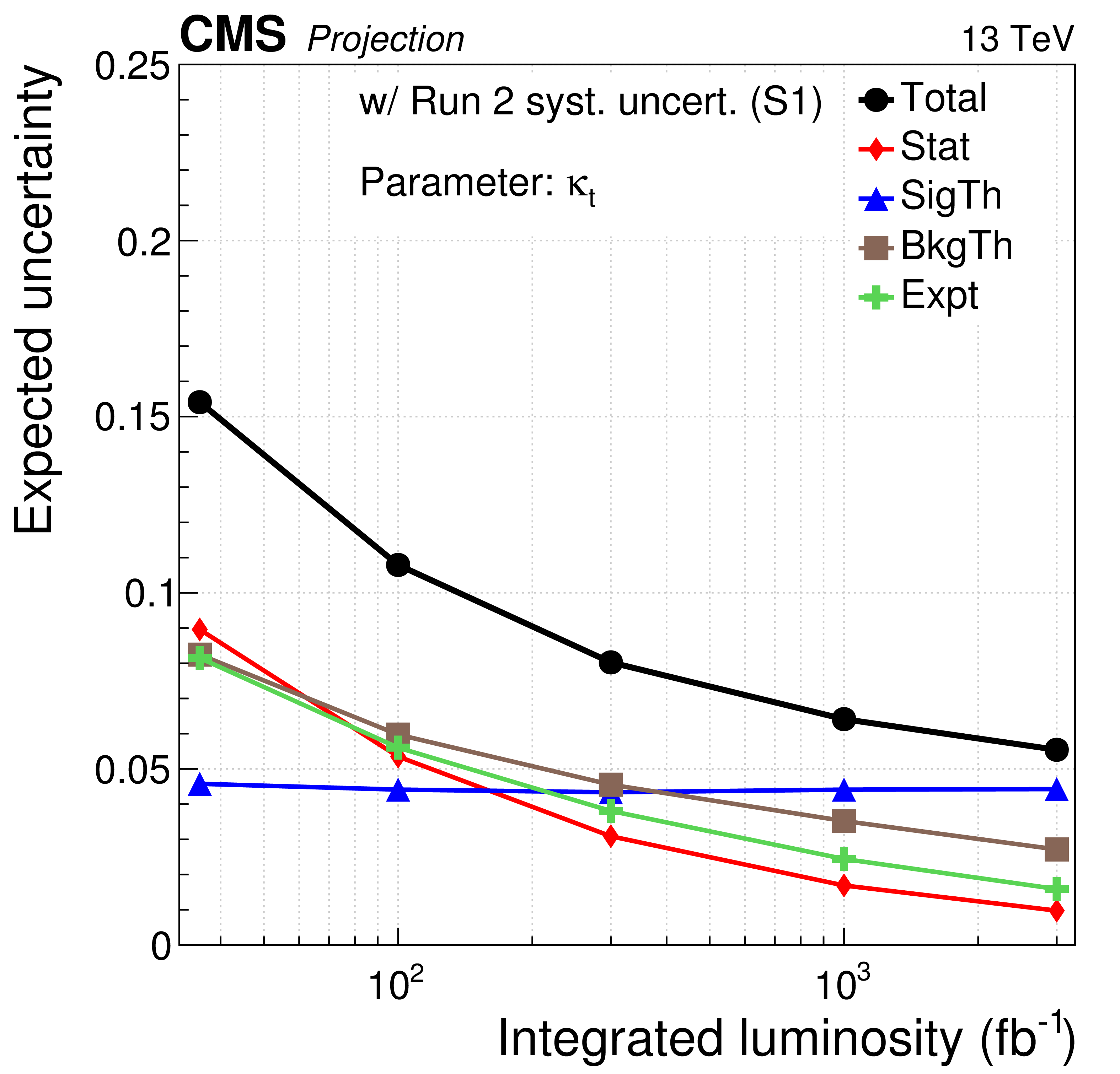
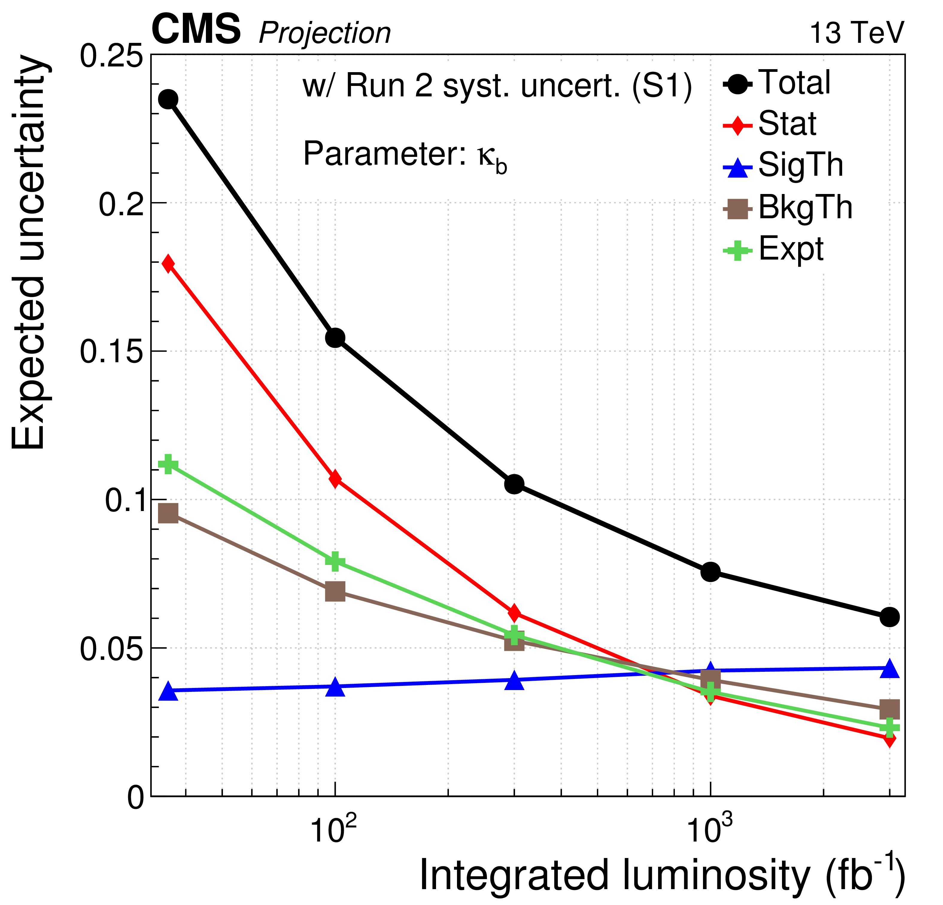
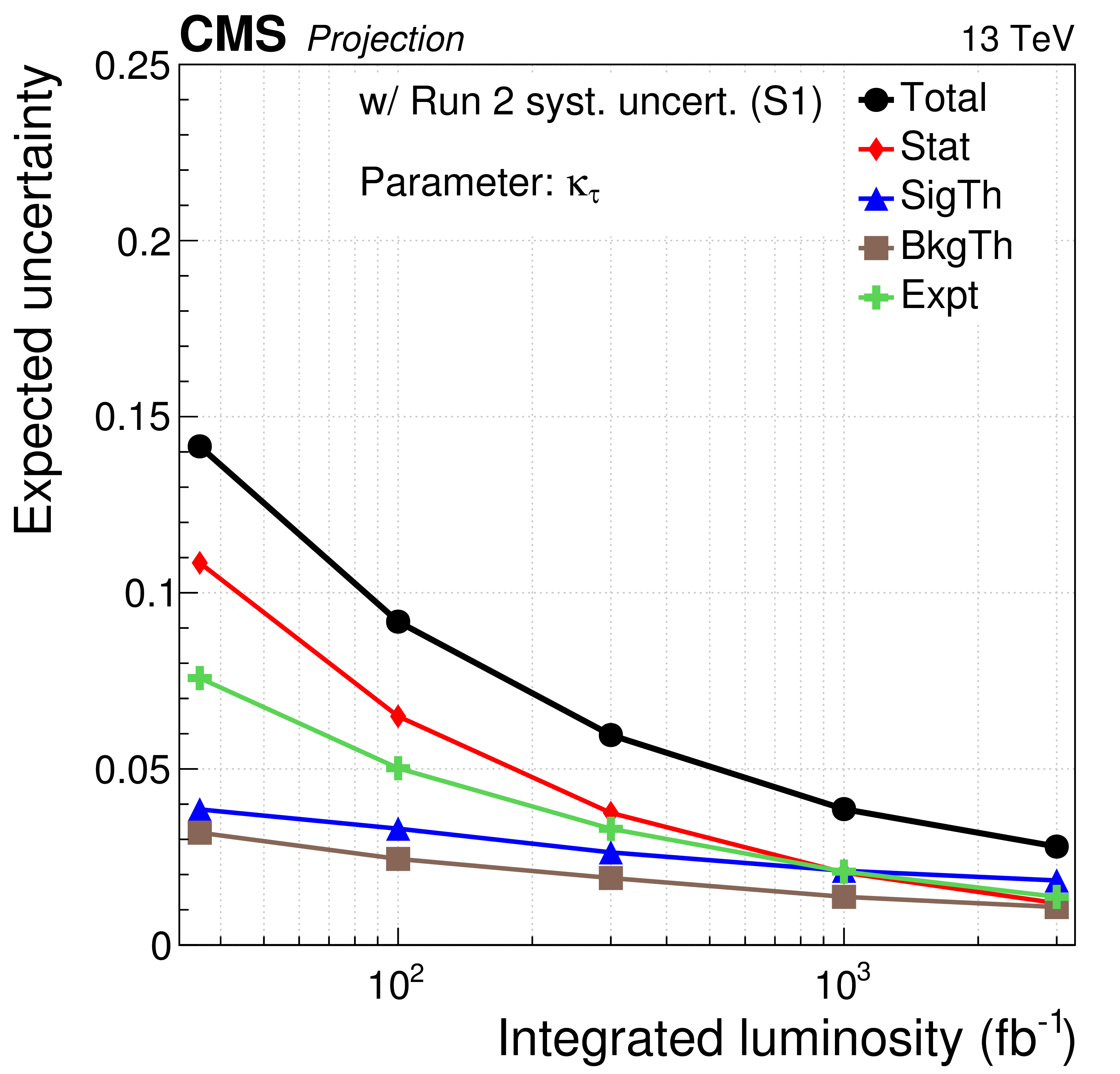
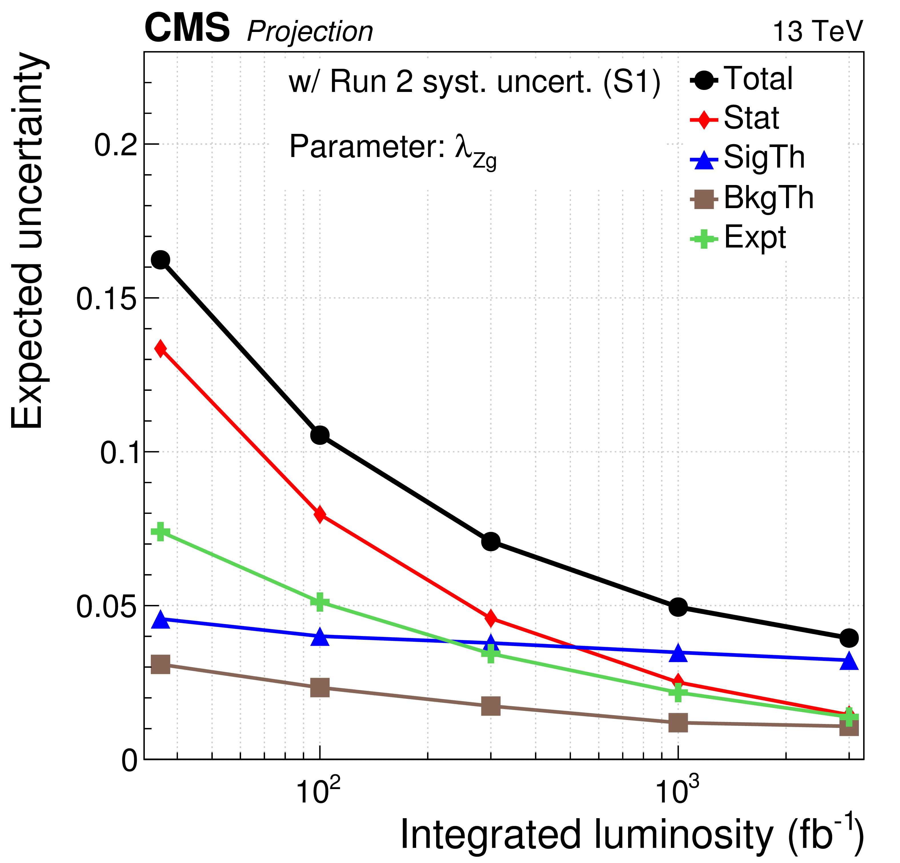
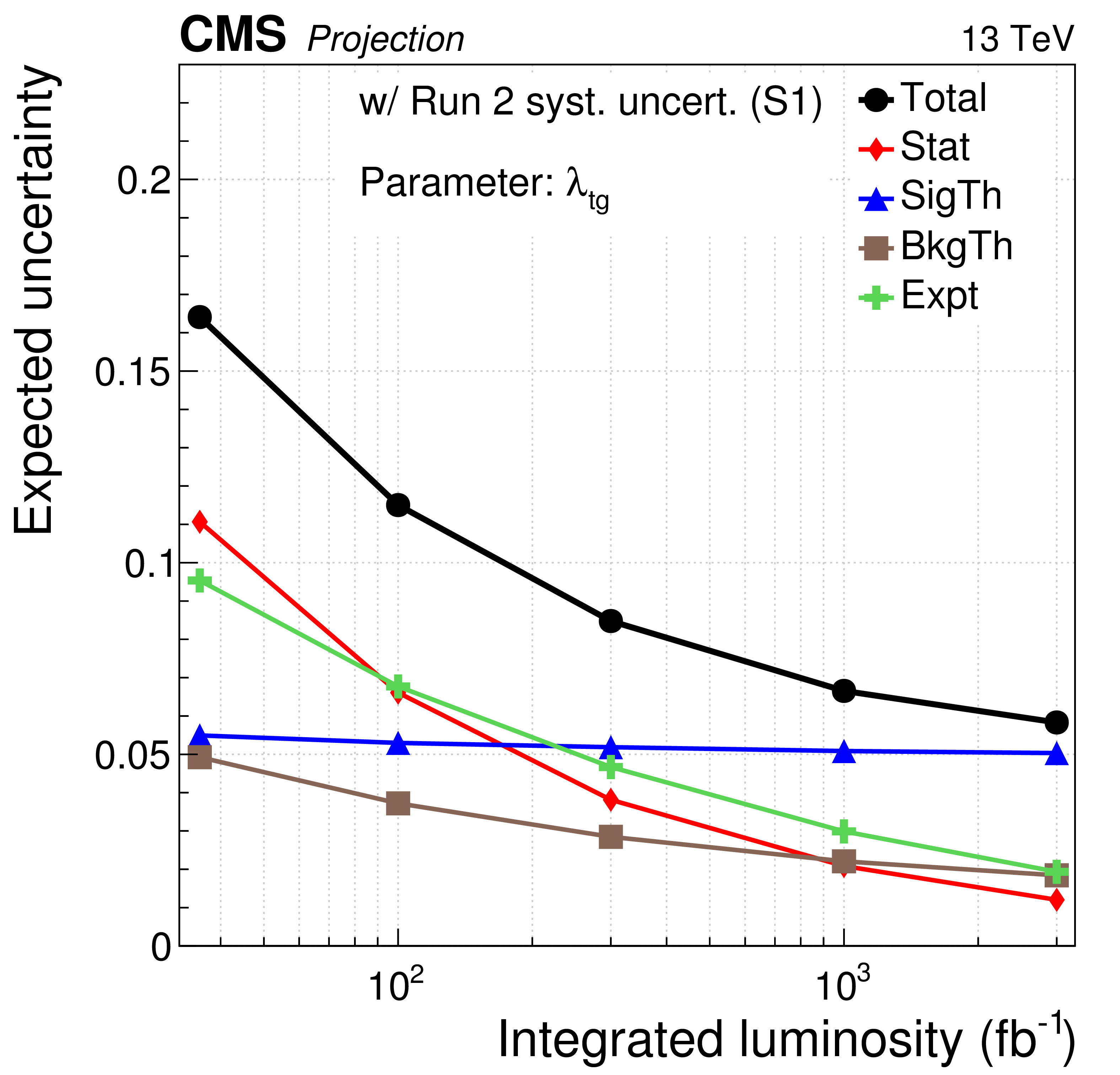
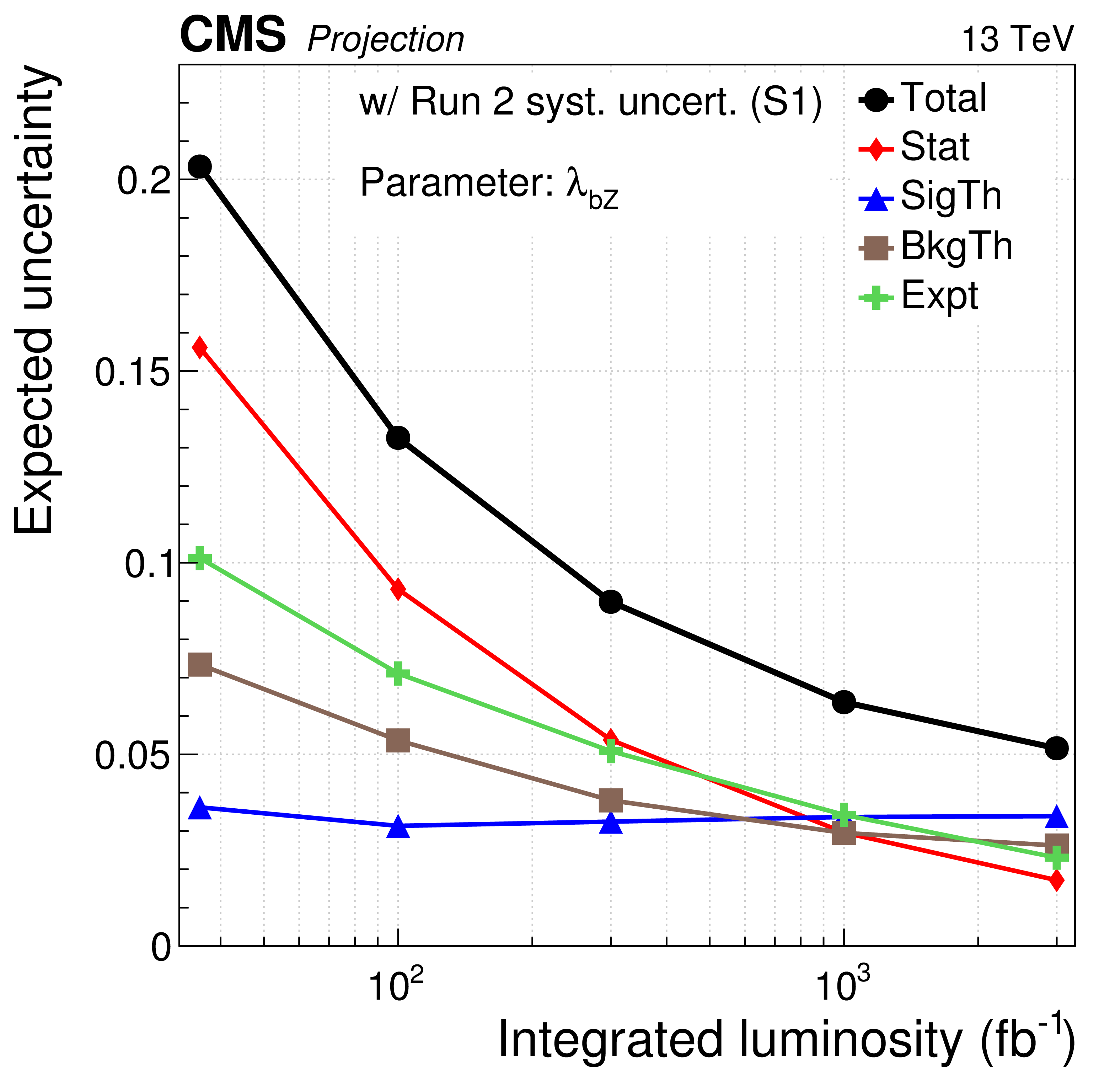
Figure 22:
Evolution of the uncertainty contribution with integrated luminosity for the coupling modifier parameters in S1 (with Run 2 systematic uncertainties [30]). |

png pdf |
Figure 22-a:
Evolution of the uncertainty contribution with integrated luminosity for the coupling modifier parameters in S1 (with Run 2 systematic uncertainties [30]). |
png pdf |
Figure 22-b:
Evolution of the uncertainty contribution with integrated luminosity for the coupling modifier parameters in S1 (with Run 2 systematic uncertainties [30]). |

png pdf |
Figure 22-c:
Evolution of the uncertainty contribution with integrated luminosity for the coupling modifier parameters in S1 (with Run 2 systematic uncertainties [30]). |

png pdf |
Figure 22-d:
Evolution of the uncertainty contribution with integrated luminosity for the coupling modifier parameters in S1 (with Run 2 systematic uncertainties [30]). |
png pdf |
Figure 22-e:
Evolution of the uncertainty contribution with integrated luminosity for the coupling modifier parameters in S1 (with Run 2 systematic uncertainties [30]). |
png pdf |
Figure 22-f:
Evolution of the uncertainty contribution with integrated luminosity for the coupling modifier parameters in S1 (with Run 2 systematic uncertainties [30]). |
png pdf |
Figure 22-g:
Evolution of the uncertainty contribution with integrated luminosity for the coupling modifier parameters in S1 (with Run 2 systematic uncertainties [30]). |

png pdf |
Figure 22-h:
Evolution of the uncertainty contribution with integrated luminosity for the coupling modifier parameters in S1 (with Run 2 systematic uncertainties [30]). |
png pdf |
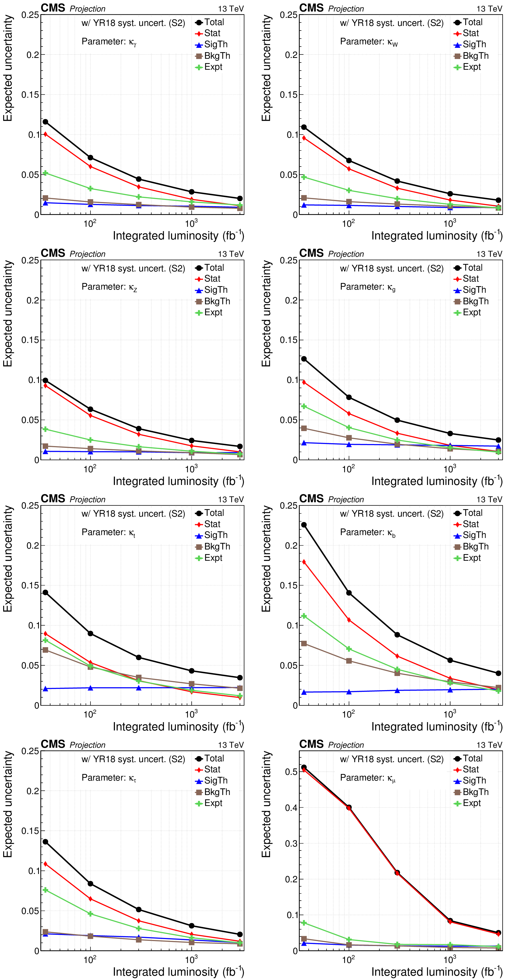
Figure 23:
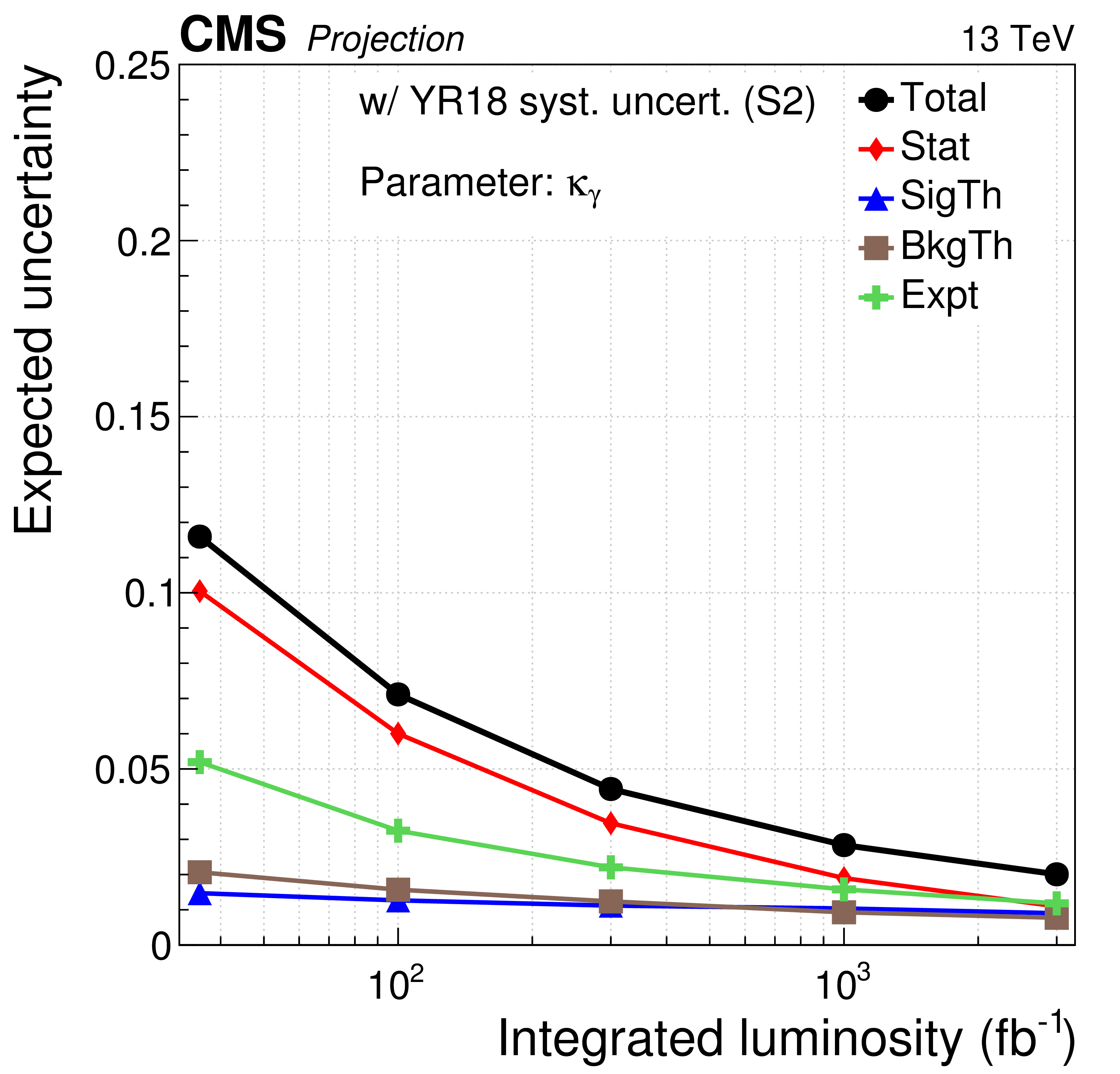
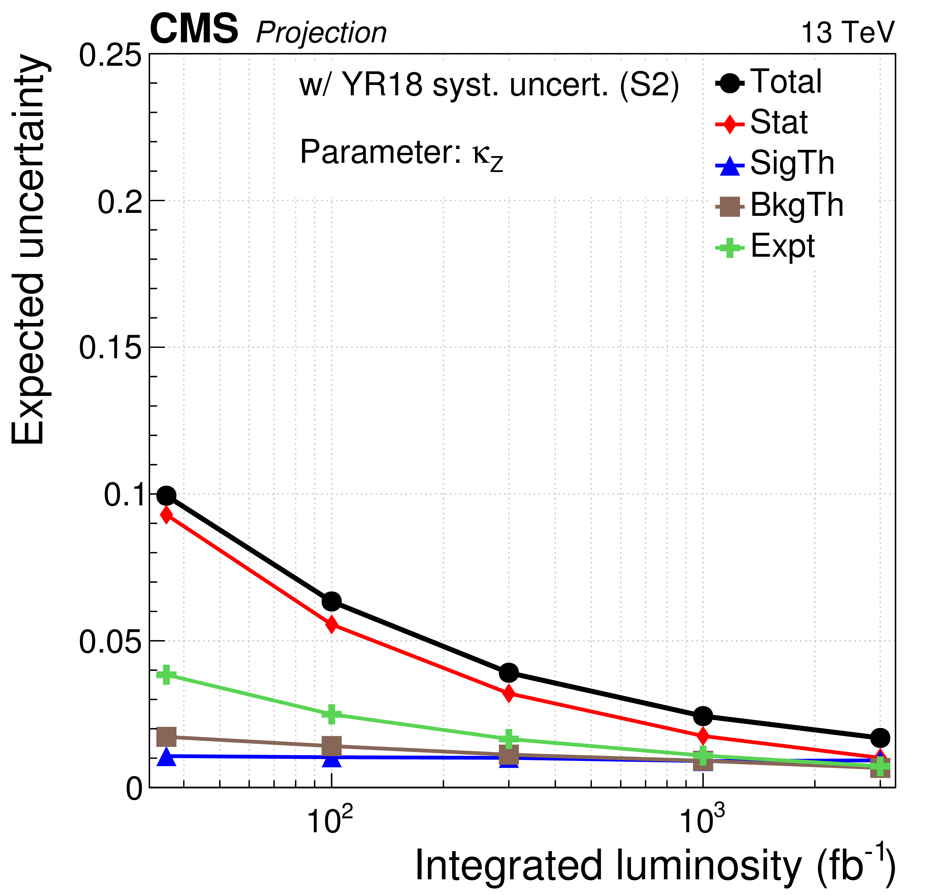
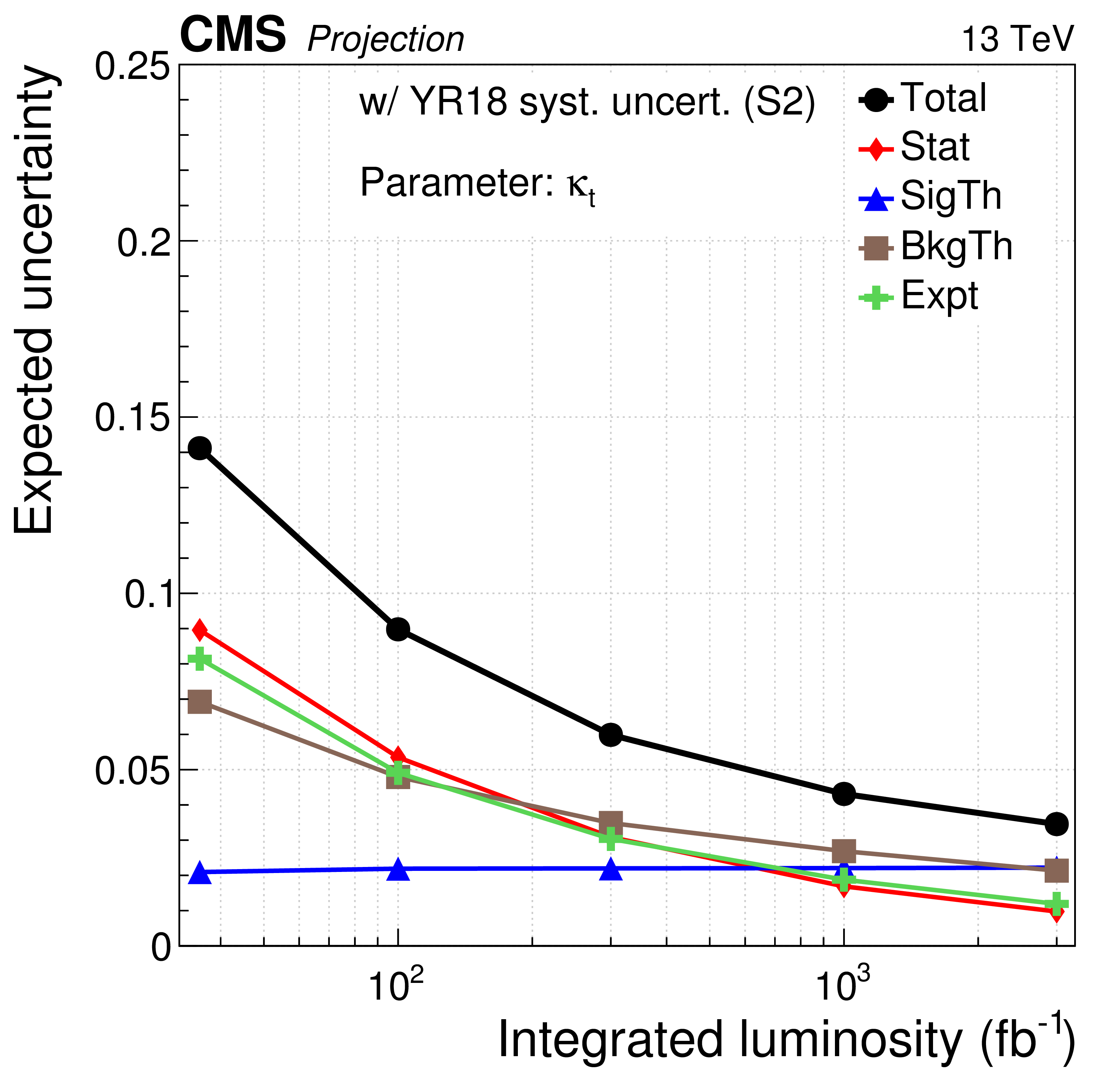
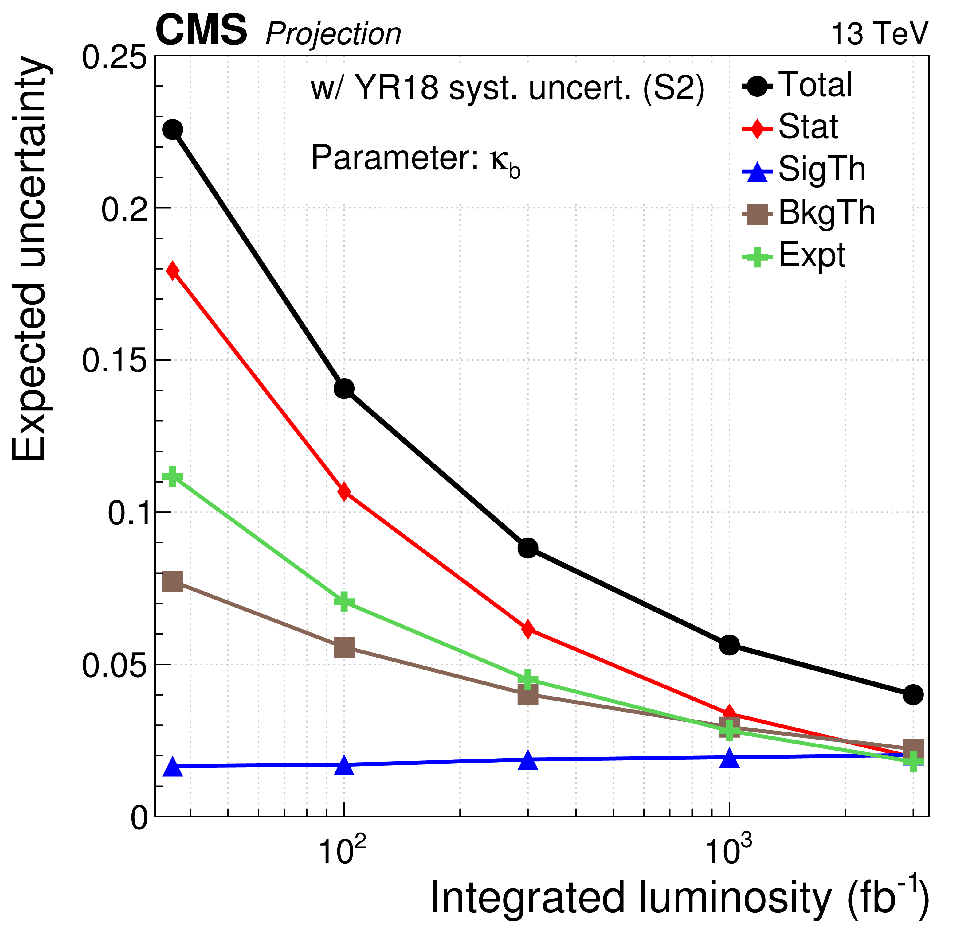
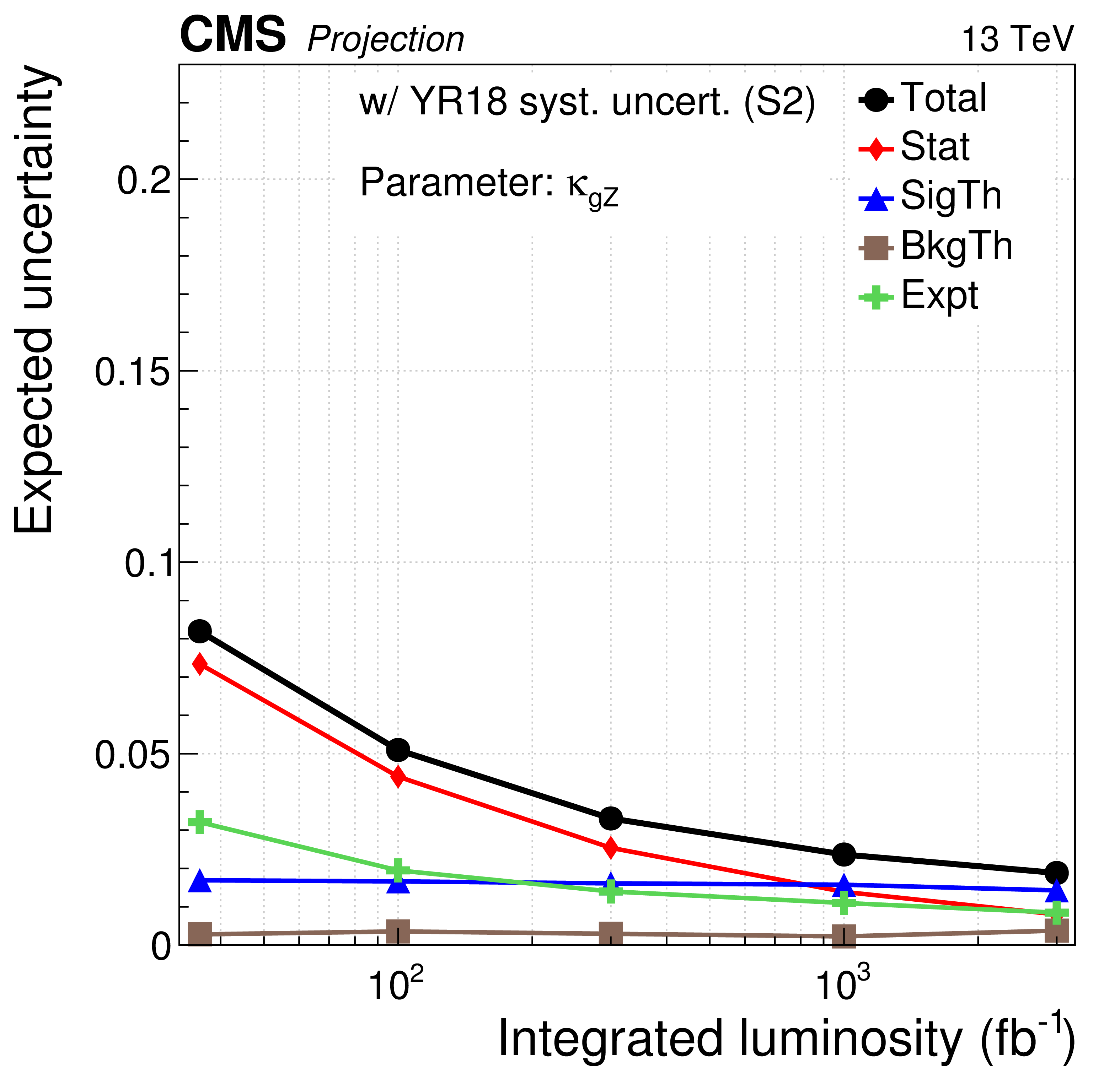
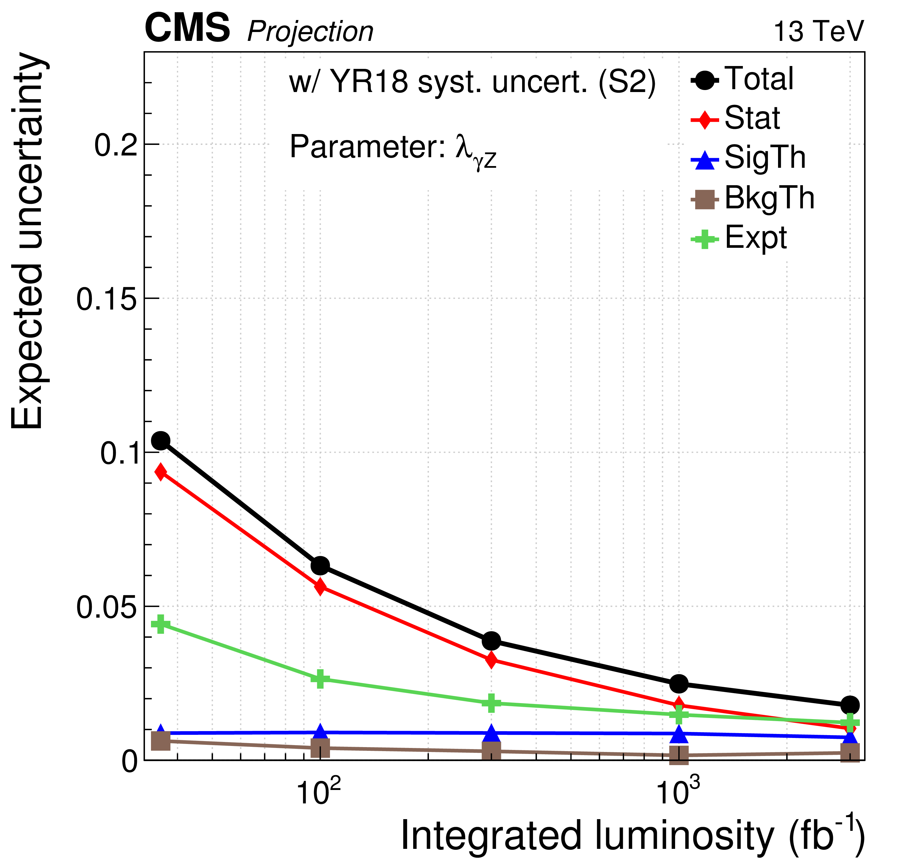
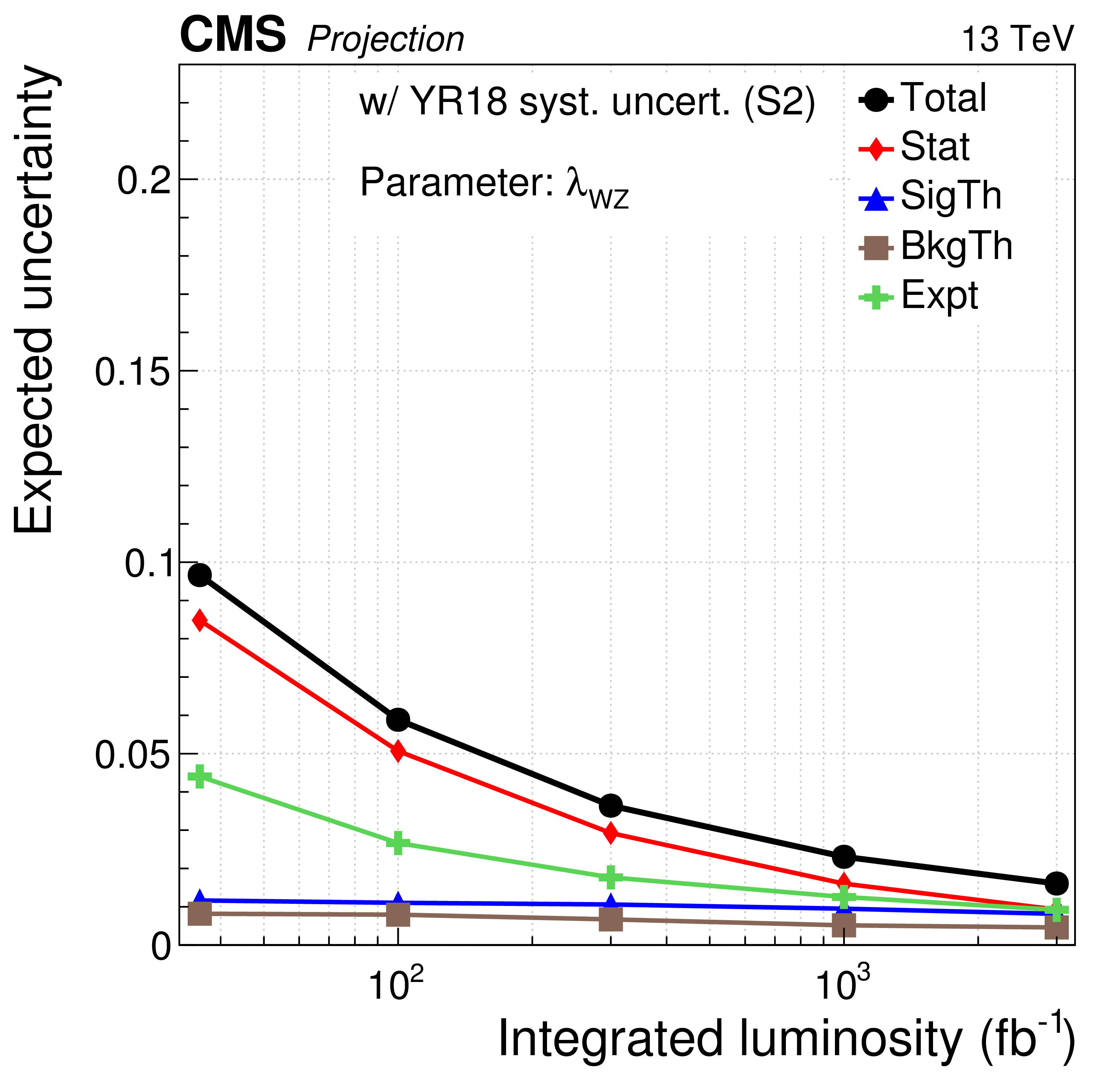
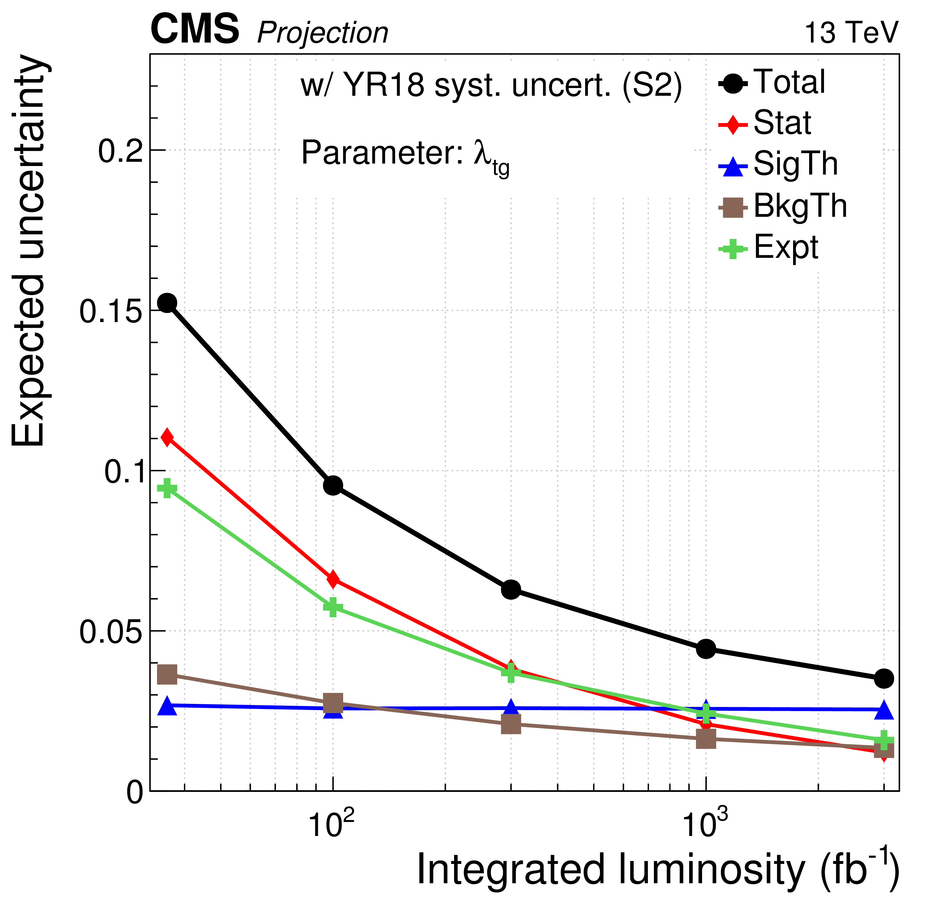
Evolution of the uncertainty contribution with integrated luminosity for the coupling modifier parameters in S2 (with YR18 systematic uncertainties). |
png pdf |
Figure 23-a:
Evolution of the uncertainty contribution with integrated luminosity for the coupling modifier parameters in S2 (with YR18 systematic uncertainties). |

png pdf |
Figure 23-b:
Evolution of the uncertainty contribution with integrated luminosity for the coupling modifier parameters in S2 (with YR18 systematic uncertainties). |
png pdf |
Figure 23-c:
Evolution of the uncertainty contribution with integrated luminosity for the coupling modifier parameters in S2 (with YR18 systematic uncertainties). |

png pdf |
Figure 23-d:
Evolution of the uncertainty contribution with integrated luminosity for the coupling modifier parameters in S2 (with YR18 systematic uncertainties). |
png pdf |
Figure 23-e:
Evolution of the uncertainty contribution with integrated luminosity for the coupling modifier parameters in S2 (with YR18 systematic uncertainties). |
png pdf |
Figure 23-f:
Evolution of the uncertainty contribution with integrated luminosity for the coupling modifier parameters in S2 (with YR18 systematic uncertainties). |

png pdf |
Figure 23-g:
Evolution of the uncertainty contribution with integrated luminosity for the coupling modifier parameters in S2 (with YR18 systematic uncertainties). |

png pdf |
Figure 23-h:
Evolution of the uncertainty contribution with integrated luminosity for the coupling modifier parameters in S2 (with YR18 systematic uncertainties). |

png pdf |
Figure 24:
Summary plot showing the total expected $ \pm $1$ \sigma $ uncertainties in S1 (with Run 2 systematic uncertainties [30]) and S2 (with YR18 systematic uncertainties) on the coupling modifier ratio parameters for 300 fb$^{-1}$ (left) and 3000 fb$^{-1}$ (right). |
png pdf |
Figure 24-a:
Summary plot showing the total expected $ \pm $1$ \sigma $ uncertainties in S1 (with Run 2 systematic uncertainties [30]) and S2 (with YR18 systematic uncertainties) on the coupling modifier ratio parameters for 300 fb$^{-1}$ (left) and 3000 fb$^{-1}$ (right). |

png pdf |
Figure 24-b:
Summary plot showing the total expected $ \pm $1$ \sigma $ uncertainties in S1 (with Run 2 systematic uncertainties [30]) and S2 (with YR18 systematic uncertainties) on the coupling modifier ratio parameters for 300 fb$^{-1}$ (left) and 3000 fb$^{-1}$ (right). |

png pdf |
Figure 25:
Evolution of the uncertainty contribution with integrated luminosity for the coupling modifier ratio parameters in S1 (with Run 2 systematic uncertainties [30]). |

png pdf |
Figure 25-a:
Evolution of the uncertainty contribution with integrated luminosity for the coupling modifier ratio parameters in S1 (with Run 2 systematic uncertainties [30]). |

png pdf |
Figure 25-b:
Evolution of the uncertainty contribution with integrated luminosity for the coupling modifier ratio parameters in S1 (with Run 2 systematic uncertainties [30]). |

png pdf |
Figure 25-c:
Evolution of the uncertainty contribution with integrated luminosity for the coupling modifier ratio parameters in S1 (with Run 2 systematic uncertainties [30]). |
png pdf |
Figure 25-d:
Evolution of the uncertainty contribution with integrated luminosity for the coupling modifier ratio parameters in S1 (with Run 2 systematic uncertainties [30]). |
png pdf |
Figure 25-e:
Evolution of the uncertainty contribution with integrated luminosity for the coupling modifier ratio parameters in S1 (with Run 2 systematic uncertainties [30]). |
png pdf |
Figure 25-f:
Evolution of the uncertainty contribution with integrated luminosity for the coupling modifier ratio parameters in S1 (with Run 2 systematic uncertainties [30]). |

png pdf |
Figure 25-g:
Evolution of the uncertainty contribution with integrated luminosity for the coupling modifier ratio parameters in S1 (with Run 2 systematic uncertainties [30]). |

png pdf |
Figure 25-h:
Evolution of the uncertainty contribution with integrated luminosity for the coupling modifier ratio parameters in S1 (with Run 2 systematic uncertainties [30]). |

png pdf |
Figure 26:
Evolution of the uncertainty contribution with integrated luminosity for the coupling modifier ratio parameters in S2 (with YR18 systematic uncertainties). |
png pdf |
Figure 26-a:
Evolution of the uncertainty contribution with integrated luminosity for the coupling modifier ratio parameters in S2 (with YR18 systematic uncertainties). |
png pdf |
Figure 26-b:
Evolution of the uncertainty contribution with integrated luminosity for the coupling modifier ratio parameters in S2 (with YR18 systematic uncertainties). |
png pdf |
Figure 26-c:
Evolution of the uncertainty contribution with integrated luminosity for the coupling modifier ratio parameters in S2 (with YR18 systematic uncertainties). |

png pdf |
Figure 26-d:
Evolution of the uncertainty contribution with integrated luminosity for the coupling modifier ratio parameters in S2 (with YR18 systematic uncertainties). |
png pdf |
Figure 26-e:
Evolution of the uncertainty contribution with integrated luminosity for the coupling modifier ratio parameters in S2 (with YR18 systematic uncertainties). |
png pdf |
Figure 26-f:
Evolution of the uncertainty contribution with integrated luminosity for the coupling modifier ratio parameters in S2 (with YR18 systematic uncertainties). |

png pdf |
Figure 26-g:
Evolution of the uncertainty contribution with integrated luminosity for the coupling modifier ratio parameters in S2 (with YR18 systematic uncertainties). |

png pdf |
Figure 26-h:
Evolution of the uncertainty contribution with integrated luminosity for the coupling modifier ratio parameters in S2 (with YR18 systematic uncertainties). |

png pdf |
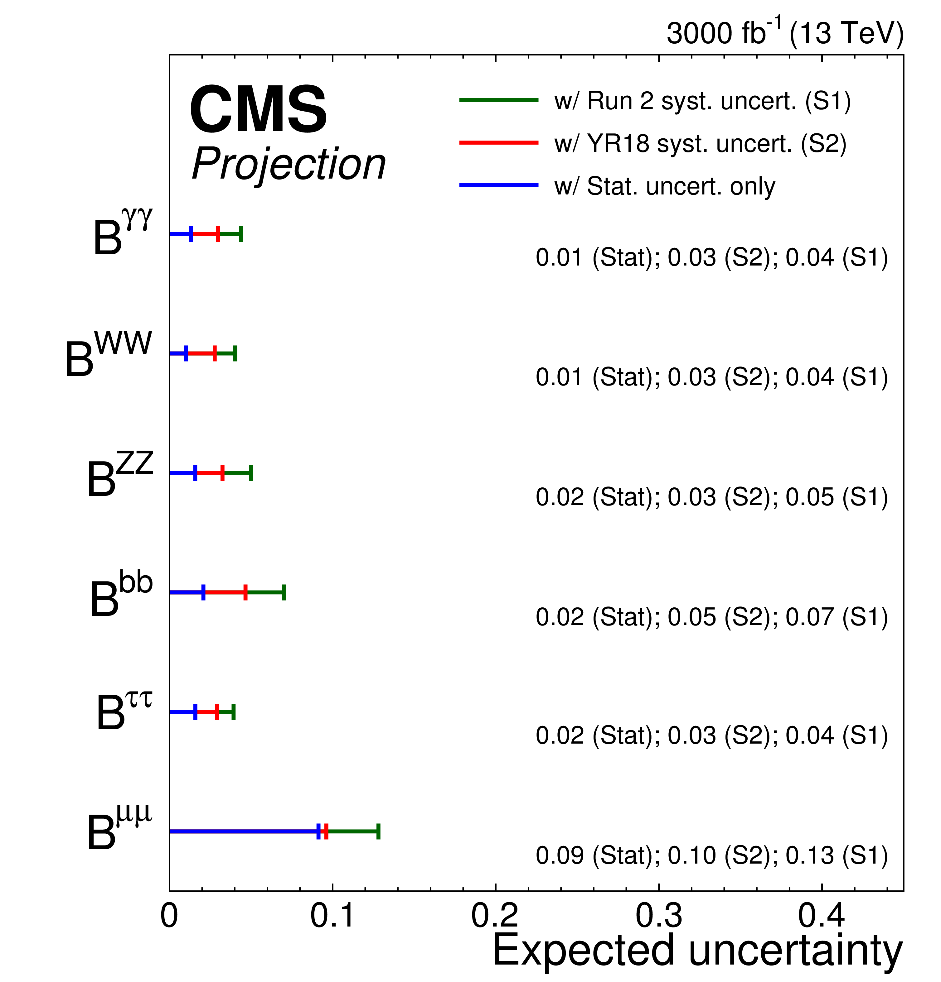
Figure 27:
Summary plot showing the total expected $ \pm $1$ \sigma $ uncertainties in S1 (with Run 2 systematic uncertainties [30]) and S2 (with YR18 systematic uncertainties) on the branching ratio measurements for 300 fb$^{-1}$ (left) and 3000 fb$^{-1}$ (right). The statistical-only component of the uncertainty is also shown. |

png pdf |
Figure 27-a:
Summary plot showing the total expected $ \pm $1$ \sigma $ uncertainties in S1 (with Run 2 systematic uncertainties [30]) and S2 (with YR18 systematic uncertainties) on the branching ratio measurements for 300 fb$^{-1}$ (left) and 3000 fb$^{-1}$ (right). The statistical-only component of the uncertainty is also shown. |
png pdf |
Figure 27-b:
Summary plot showing the total expected $ \pm $1$ \sigma $ uncertainties in S1 (with Run 2 systematic uncertainties [30]) and S2 (with YR18 systematic uncertainties) on the branching ratio measurements for 300 fb$^{-1}$ (left) and 3000 fb$^{-1}$ (right). The statistical-only component of the uncertainty is also shown. |

png pdf |
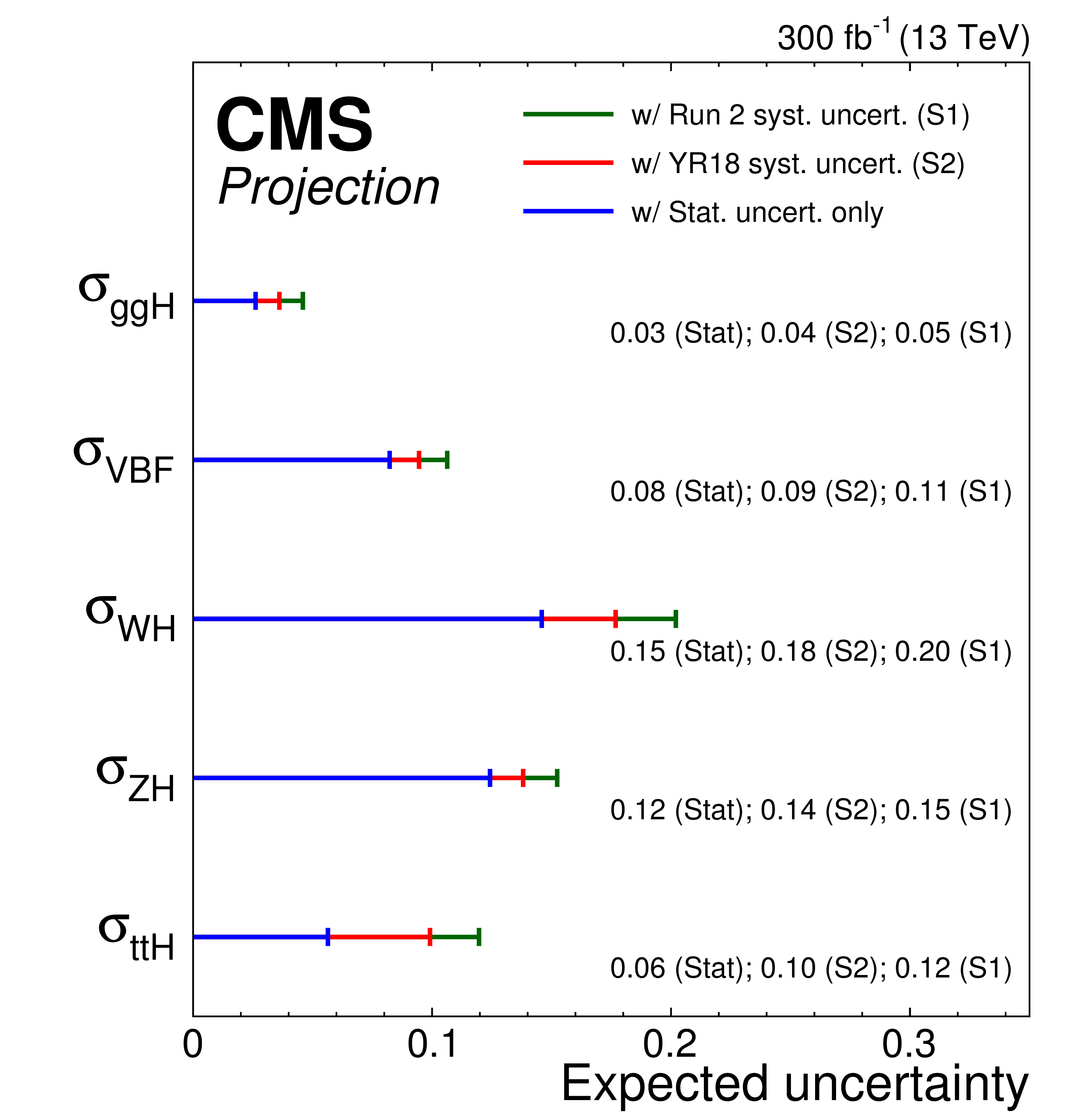
Figure 28:
Summary plot showing the total expected $ \pm $1$ \sigma $ uncertainties in S1 (with Run 2 systematic uncertainties [30]) and S2 (with YR18 systematic uncertainties) on the cross section measurements for 300 fb$^{-1}$ (left) and 3000 fb$^{-1}$ (right). The statistical-only component of the uncertainty is also shown. |
png pdf |
Figure 28-a:
Summary plot showing the total expected $ \pm $1$ \sigma $ uncertainties in S1 (with Run 2 systematic uncertainties [30]) and S2 (with YR18 systematic uncertainties) on the cross section measurements for 300 fb$^{-1}$ (left) and 3000 fb$^{-1}$ (right). The statistical-only component of the uncertainty is also shown. |

png pdf |
Figure 28-b:
Summary plot showing the total expected $ \pm $1$ \sigma $ uncertainties in S1 (with Run 2 systematic uncertainties [30]) and S2 (with YR18 systematic uncertainties) on the cross section measurements for 300 fb$^{-1}$ (left) and 3000 fb$^{-1}$ (right). The statistical-only component of the uncertainty is also shown. |
| Tables | |
png pdf |
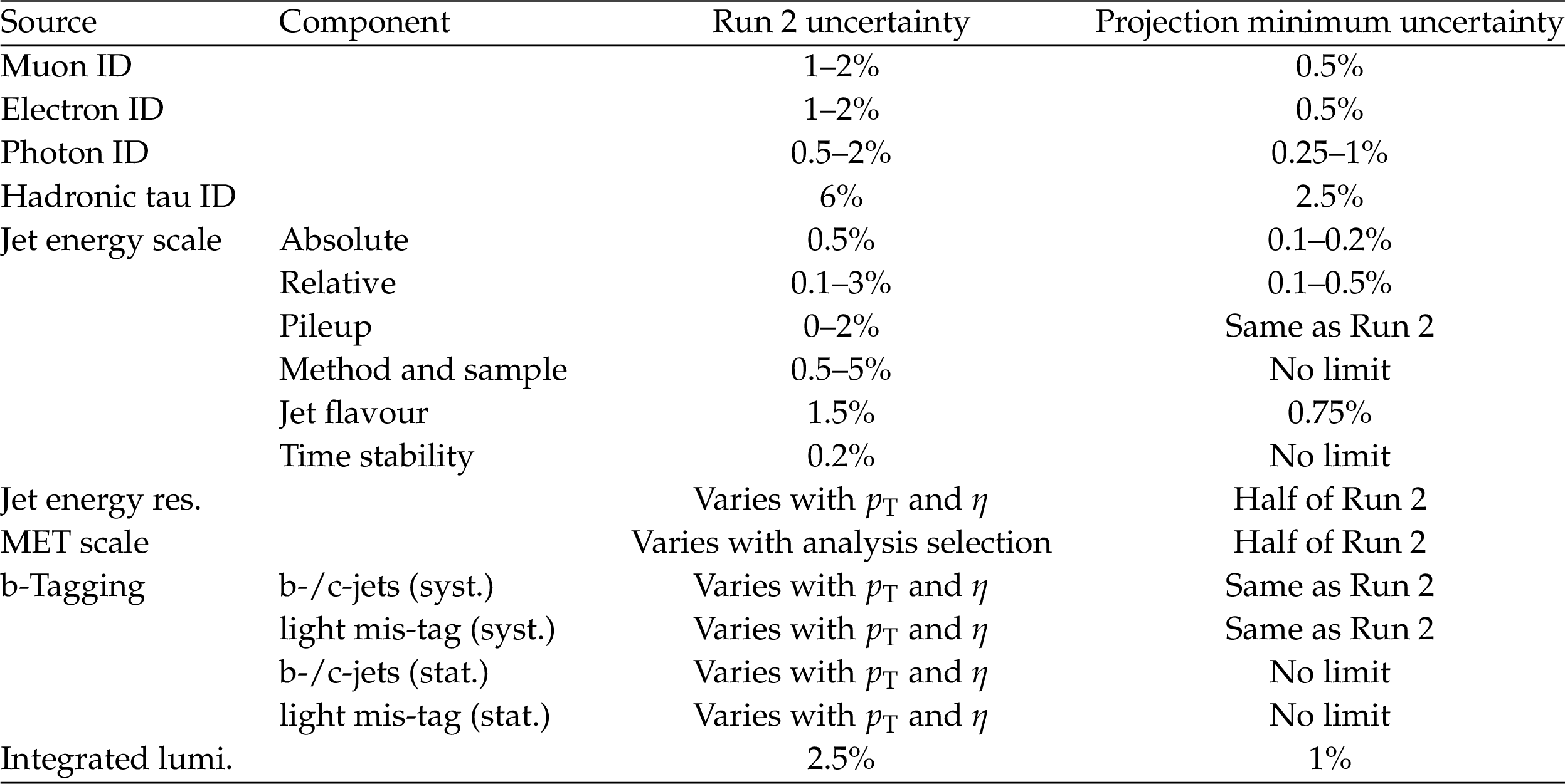
Table 1:
The sources of systematic uncertainty for which minimum values are applied in S2. |

png pdf |
Table 2:
The expected $ \pm $1$ \sigma $ uncertainties, expressed as percentages, on the per-decay-mode signal strength parameters. Values are given for both S1 (with Run 2 systematic uncertainties [30]) and S2 (with YR18 systematic uncertainties). The total uncertainty is decomposed into four components: statistical (Stat), signal theory (SigTh), background theory (BkgTh) and experimental (Exp). |

png pdf |
Table 3:
The expected $ \pm $1$ \sigma $ uncertainties, expressed as percentages, on the per-production-mode signal strength parameters. Values are given for both S1 (with Run 2 systematic uncertainties [30]) and S2 (with YR18 systematic uncertainties). The total uncertainty is decomposed into four components: statistical (Stat), signal theory (SigTh), background theory (BkgTh) and experimental (Exp). |

png pdf |
Table 4:
The expected $ \pm $1$ \sigma $ uncertainties, expressed as percentages, on the coupling modifier parameters, as well as $ {\mathrm {B_{BSM}}} $ and $ {\Gamma _{{\mathrm {H}}}/\Gamma _{{\mathrm {H}}}^{\mathrm {SM}}} $. The values for the $ {\mathrm {B_{BSM}}} $ parameter correspond to the $+1\sigma $ uncertainties only. Values are given for both S1 (with Run 2 systematic uncertainties [30]) and S2 (with YR18 systematic uncertainties). The total uncertainty is decomposed into four components: statistical (Stat), signal theory (SigTh), background theory (BkgTh) and experimental (Exp). |

png pdf |
Table 5:
Breakdown of the contributions to the expected uncertainties on the ttH signal-strength $\mu $ at different luminosities for S1 (with Run 2 systematic uncertainties [27]) and S2 (with YR18 systematic uncertainties). The uncertainties are given in percent relative to $\mu =$ 1. Results with 35.9 fb$^{-1}$ are intended for comparison with the projections to higher luminosities and differ in parts from [27] for consistency with the projected results: uncertainties due to the limited number of MC events have been omitted and theory systematic uncertainties have been halved in case of the scenario S2. |

png pdf |
Table 6:
Contributions of particular groups of uncertainties, expressed as percentages, at an integrated luminosity of 3000 fb$^{-1}$ in S1 (with Run 2 systematic uncertainties [24]) and S2 (with YR18 systematic uncertainties). The total uncertainty is decomposed into four components: signal theory, background theory, experimental and statistical. The signal theory uncertainty is further split into inclusive and acceptance parts, and the contributions of the b tagging and JES/JER uncertainties to the experimental component are also given. |

png pdf |
Table 7:
The $ \pm $1$ \sigma $ uncertainties on expected $\mu _{{{\mathrm {t}} {\mathrm {H}}}}$=1 for scenarios S1 (with Run 2 systematic uncertainties [38]) and S2 (with YR18 systematic uncertainties) at all three luminosities, considering also the case when $\mu _{{\mathrm{t} \mathrm{t} {\mathrm {H}}}}$ is fixed at the SM value. |

png pdf |
Table 8:
Relative uncertainties on the projected $ {{p_{\mathrm {T}}} ({\mathrm {H}})} $ spectrum under S1 (with Run 2 systematic uncertainties [41]) at 3000 fb$^{-1}$ . |

png pdf |
Table 9:
Relative uncertainties on the projected $ {{p_{\mathrm {T}}} ({\mathrm {H}})} $ spectrum under S2 (with YR18 systematic uncertainties) at 3000 fb$^{-1}$ . |

png pdf |
Table 10:
Summary of the 95% CL intervals for ${{f_{a 3}} {\cos\left ({\phi _{a 3}} \right)}}$, under the assumption $ {\Gamma _ {\mathrm {H}}} = {\Gamma _ {\mathrm {H}} ^{\mathrm {SM}}} $, and for ${\Gamma _ {\mathrm {H}}}$ under the assumption $ {f_{a i}} =$ 0 for projections at 3000 fb$^{-1}$ . Constraints on ${{f_{a 3}} {\cos\left ({\phi _{a 3}} \right)}}$ are multiplied by $10^{4}$. Values are given for scenarios S1 (with Run 2 systematic uncertainties [47]) and the approximate S2 scenario, as described in the text. |

png pdf |
Table 11:
The expected $ \pm $1$ \sigma $ uncertainties, expressed as percentages, on the coupling modifier ratio parameters. Values are given for both S1 (with Run 2 systematic uncertainties [30]) and S2 (with YR18 systematic uncertainties). The total uncertainty is decomposed into four components: statistical (Stat), signal theory (SigTh), background theory (BkgTh) and experimental (Exp). |

png pdf |
Table 12:
The expected $ \pm $1$ \sigma $ uncertainties on the branching ratio measurements, expressed as percentages, and assuming the SM values for the production cross sections. Values are given for both S1 (with Run 2 systematic uncertainties [30]) and S2 (with YR18 systematic uncertainties). The total uncertainty is decomposed into four components: statistical (Stat), signal theory (SigTh), background theory (BkgTh) and experimental (Exp). The theory uncertainties on the branching ratios are neglected in these results. |
png pdf |
Table 13:
The expected $ \pm $1$ \sigma $ uncertainties on the cross section measurements, expressed as percentages, and assuming the SM values for the branching fractions. Values are given for both S1 (with Run 2 systematic uncertainties [30]) and S2 (with YR18 systematic uncertainties). The total uncertainty is decomposed into four components: statistical (Stat), signal theory (SigTh), background theory (BkgTh) and experimental (Exp). The theory uncertainties on the production cross sections are neglected in these results. |
| Summary |
|
The discovery of the Higgs boson opened a new era of precision measurements of the properties of the new particle, aimed to thoroughly test their consistency with the SM predictions. The present measurements of the Higgs boson couplings to fermions, bosons and of the tensor structure of the Higgs boson interaction with electroweak gauge bosons show no significant deviations with respect to the SM expectations. The HL-LHC will provide a unique environment in which to test the Higgs boson properties. This summary describes the projected sensitivity to 300 and 3000 fb$^{-1}$ of several Higgs boson analyses performed on the 13 TeV data set collected in 2016. The projections are performed under different scenarios considering the systematic uncertainties under Run 2 and HL-LHC conditions. Results have been presented for a combined measurement of coupling modifiers and signal strengths, with additional studies for ttH and VH production with $\text{H}\to\text{bb}$ decay, and for production in association with a single top quark. Projections have also been given for the measurement of the Higgs boson transverse momentum differential cross section, and the expected constraints on anomalous couplings and the total width using on- and off-shell $\text{H}\to\text{ZZ}$ measurements. |
| Additional Figures | |

png pdf |
Additional Figure 1:
Total post-fit uncertainty on $\mu $ as a function of the prior $ {\mathrm{t} \mathrm{t} \text {+}\text {HF}} $ background normalisation uncertainty expected at 35.9 fb$^{-1}$ (left) and at 3000 fb$^{-1}$ (right). The point at 50% prior $ {\mathrm{t} \mathrm{t} \text {+}\text {HF}} $ uncertainty corresponds to the nominal fit model; at the other points, the prior $ {\mathrm{t} \mathrm{t} \text {+}\text {HF}} $ cross-section uncertainty (all four nuisance parameters for ${\mathrm{t} \mathrm{t} \text {+}\mathrm{b} \mathrm{b}}$, ${\mathrm{t} \mathrm{t} \text {+}\mathrm{b}}$, ${\mathrm{t} \mathrm{t} \text {+2}\mathrm{b}}$, and ${\mathrm{t} \mathrm{t} \text {+}\mathrm{c} \mathrm{c}}$) has been reduced as indicated on the x-axis. In each case, all other uncertainties follow the {\text {S2}} scenario. |
png pdf |
Additional Figure 1-a:
Total post-fit uncertainty on $\mu $ as a function of the prior $ {\mathrm{t} \mathrm{t} \text {+}\text {HF}} $ background normalisation uncertainty expected at 35.9 fb$^{-1}$ (left) and at 3000 fb$^{-1}$ (right). The point at 50% prior $ {\mathrm{t} \mathrm{t} \text {+}\text {HF}} $ uncertainty corresponds to the nominal fit model; at the other points, the prior $ {\mathrm{t} \mathrm{t} \text {+}\text {HF}} $ cross-section uncertainty (all four nuisance parameters for ${\mathrm{t} \mathrm{t} \text {+}\mathrm{b} \mathrm{b}}$, ${\mathrm{t} \mathrm{t} \text {+}\mathrm{b}}$, ${\mathrm{t} \mathrm{t} \text {+2}\mathrm{b}}$, and ${\mathrm{t} \mathrm{t} \text {+}\mathrm{c} \mathrm{c}}$) has been reduced as indicated on the x-axis. In each case, all other uncertainties follow the {\text {S2}} scenario. |
png pdf |
Additional Figure 1-b:
Total post-fit uncertainty on $\mu $ as a function of the prior $ {\mathrm{t} \mathrm{t} \text {+}\text {HF}} $ background normalisation uncertainty expected at 35.9 fb$^{-1}$ (left) and at 3000 fb$^{-1}$ (right). The point at 50% prior $ {\mathrm{t} \mathrm{t} \text {+}\text {HF}} $ uncertainty corresponds to the nominal fit model; at the other points, the prior $ {\mathrm{t} \mathrm{t} \text {+}\text {HF}} $ cross-section uncertainty (all four nuisance parameters for ${\mathrm{t} \mathrm{t} \text {+}\mathrm{b} \mathrm{b}}$, ${\mathrm{t} \mathrm{t} \text {+}\mathrm{b}}$, ${\mathrm{t} \mathrm{t} \text {+2}\mathrm{b}}$, and ${\mathrm{t} \mathrm{t} \text {+}\mathrm{c} \mathrm{c}}$) has been reduced as indicated on the x-axis. In each case, all other uncertainties follow the {\text {S2}} scenario. |

png pdf |
Additional Figure 2:
Correlation coefficients ($\rho $) between parameters in the signal strength per-production-and-decay parametrisation for S2 (with YR18 systematic uncertainties) at 3000 fb$^{-1}$. |
| Additional Tables | |
png pdf |
Additional Table 1:
The expected $ \pm $1$ \sigma $ uncertainties, expressed as percentages, on the per-production-and-decay signal strength parameters. Values are given for both S1 and S2. The total uncertainty is decomposed into four components: statistical (Stat), signal theory (SigTh), background theory (BkgTh) and experimental (Exp). |
| References | ||||
| 1 | ATLAS Collaboration | Observation of a new particle in the search for the standard model higgs boson with the atlas detector at the lhc | PLB 716 (2012) 129 | |
| 2 | CMS Collaboration | Observation of a new boson at a mass of 125~GeV with the CMS experiment at the LHC | PLB 716 (2012) 3061 | |
| 3 | CMS Collaboration | Observation of a new boson with mass near 125 GeV in pp collisions at $ \sqrt{s} = $ 7 and 8 TeV | JHEP 06 (2013) 081 | CMS-HIG-12-036 1303.4571 |
| 4 | CMS Collaboration | The CMS Experiment at the CERN LHC | JINST 3 (2008) S08004 | CMS-00-001 |
| 5 | G. Apollinari et al. | High-Luminosity Large Hadron Collider (HL-LHC) : Preliminary Design Report | ||
| 6 | CMS Collaboration | Technical Proposal for the Phase-II Upgrade of the CMS Detector | CMS-PAS-TDR-15-002 | CMS-PAS-TDR-15-002 |
| 7 | CMS Collaboration | The Phase-2 Upgrade of the CMS Tracker | CDS | |
| 8 | CMS Collaboration | The Phase-2 Upgrade of the CMS Barrel Calorimeters Technical Design Report | CDS | |
| 9 | CMS Collaboration | The Phase-2 Upgrade of the CMS Endcap Calorimeter | CDS | |
| 10 | CMS Collaboration | The Phase-2 Upgrade of the CMS Muon Detectors | CDS | |
| 11 | CMS Collaboration | CMS Phase-2 Object Performance | ||
| 12 | DELPHES 3 Collaboration | DELPHES 3, A modular framework for fast simulation of a generic collider experiment | JHEP 02 (2014) 057 | 1307.6346 |
| 13 | CMS Collaboration | Projected Performance of an Upgraded CMS Detector at the LHC and HL-LHC: Contribution to the Snowmass Process | in Proceedings, Community Summer Study 2013: Snowmass on the Mississippi (CSS2013): Minneapolis, MN, USA, July 29-August 6, 2013 2013 | 1307.7135 |
| 14 | CMS Collaboration | Projected performance of Higgs analyses at the HL-LHC for ECFA 2016 | CMS-PAS-FTR-16-002 | CMS-PAS-FTR-16-002 |
| 15 | LHC Higgs Cross Section Working Group Collaboration | Handbook of LHC Higgs Cross Sections: 4. Deciphering the Nature of the Higgs Sector | 1610.07922 | |
| 16 | ATLAS and CMS Collaborations, LHC Higgs Combination Group | Procedure for the LHC Higgs boson search combination in Summer 2011 | ATL-PHYS-PUB 2011-11, CMS NOTE 2011/005 | |
| 17 | W. Verkerke and D. P. Kirkby | The RooFit toolkit for data modeling | in 13$^\textth$ International Conference for Computing in High Energy and Nuclear Physics (CHEP03) 2003 CHEP-2003-MOLT007 | physics/0306116 |
| 18 | L. Moneta et al. | The RooStats Project | PoS ACAT2010 (2010) 57 | 1009.1003 |
| 19 | G. Cowan, K. Cranmer, E. Gross, and O. Vitells | Asymptotic formulae for likelihood-based tests of new physics | EPJC 71 (2011) 1554 | 1007.1727 |
| 20 | CMS Collaboration | Measurements of Higgs boson properties in the diphoton decay channel in proton-proton collisions at $ \sqrt{s} = $ 13 TeV | Accepted by JHEP | CMS-HIG-16-040 1804.02716 |
| 21 | CMS Collaboration | Measurements of properties of the Higgs boson decaying into the four-lepton final state in pp collisions at $ \sqrt{s}= $ 13 ~TeV | JHEP 11 (2017) 47 | CMS-HIG-16-041 1706.09936 |
| 22 | CMS Collaboration | Measurements of properties of the Higgs boson decaying to a W boson pair in pp collisions at $ \sqrt{s}= $ 13 TeV | Submitted to PLB | CMS-HIG-16-042 1806.05246 |
| 23 | CMS Collaboration | Observation of the Higgs boson decay to a pair of $ \tau $ leptons with the CMS detector | PLB 779 (2018) 283 | CMS-HIG-16-043 1708.00373 |
| 24 | CMS Collaboration | Evidence for the Higgs boson decay to a bottom quark-antiquark pair | PLB 780 (2018) 501 | CMS-HIG-16-044 1709.07497 |
| 25 | CMS Collaboration | Inclusive search for a highly boosted Higgs boson decaying to a bottom quark-antiquark pair | PRL 120 (2018) 071802 | CMS-HIG-17-010 1709.05543 |
| 26 | CMS Collaboration | Evidence for associated production of a Higgs boson with a top quark pair in final states with electrons, muons, and hadronically decaying $ \tau $ leptons at $ \sqrt{s} = $ 13 TeV | JHEP 08 (2018) 066 | CMS-HIG-17-018 1803.05485 |
| 27 | CMS Collaboration | Search for $ \mathrm{t\overline{t}} $H production in the $ \mathrm{H}\to\mathrm{b\overline{b}} $ decay channel with leptonic $ \mathrm{t\overline{t}} $ decays in proton-proton collisions at $ \sqrt{s} = $ 13 TeV | Submitted to JHEP | CMS-HIG-17-026 1804.03682 |
| 28 | CMS Collaboration | Search for $ \mathrm{t}\overline{\mathrm{t}} $H production in the all-jet final state in proton-proton collisions at $ \sqrt{s}= $ 13 TeV | JHEP 06 (2018) 101 | CMS-HIG-17-022 1803.06986 |
| 29 | CMS Collaboration | Search for the Higgs boson decaying to two muons in proton-proton collisions at $ \sqrt{s}= $ 13 TeV | Accepted by PRLett | CMS-HIG-17-019 1807.06325 |
| 30 | CMS Collaboration | Combined measurements of Higgs boson couplings in proton-proton collisions at $ \sqrt{s}= $ 13 TeV | \emphSubmitted to EPJC | CMS-HIG-17-031 1809.10733 |
| 31 | LHC Higgs Cross Section Working Group | Handbook of LHC Higgs Cross Sections: 3. Higgs Properties | 1307.1347 | |
| 32 | CMS Collaboration | Observation of $ \mathrm{t\overline{t}} $H production | PRL 120 (2018) 231801 | CMS-HIG-17-035 1804.02610 |
| 33 | CMS Collaboration | Measurements of $ \mathrm{t\bar{t}} $ cross sections in association with b jets and inclusive jets and their ratio using dilepton final states in pp collisions at $ \sqrt{s} = $ 13 TeV | PLB 776 (2018) 355 | CMS-TOP-16-010 1705.10141 |
| 34 | G. Bevilacqua, M. V. Garzelli, and A. Kardos | $ \text{t}\overline{\text{t}}\text{b}\overline{\text{b}} $ hadroproduction with massive bottom quarks with PowHel | 1709.06915 | |
| 35 | T. Jezo, J. M. Lindert, N. Moretti, and S. Pozzorini | New NLOPS predictions for $ \mathrm{t\bar{t}}\text{+b-jet} $ production at the LHC | 1802.00426 | |
| 36 | ATLAS Collaboration | Observation of $ H \rightarrow b\bar{b} $ decays and $ VH $ production with the ATLAS detector | PLB786 (2018) 59--86 | 1808.08238 |
| 37 | CMS Collaboration | Observation of Higgs boson decay to bottom quarks | PRL 121 (2018) 121801 | CMS-HIG-18-016 1808.08242 |
| 38 | CMS Collaboration | Search for the associated production of a Higgs boson and a single top quark in pp collisions at $ \sqrt{s} = 13 \mathrm{TeV} $ | CMS-PAS-HIG-18-009 | CMS-PAS-HIG-18-009 |
| 39 | CMS Collaboration | Search for production of a Higgs boson and a single top quark in multilepton final states in proton collisions at $ \sqrt{s}= $ 13 TeV | CMS-PAS-HIG-17-005 | CMS-PAS-HIG-17-005 |
| 40 | CMS Collaboration | Search for the th($ \mathrm{H\rightarrow b\bar{b}} $) process at $ \sqrt{s} = $ 13 TeV and study of higgs boson couplings | ||
| 41 | CMS Collaboration | Combined measurement and interpretation of differential Higgs boson production cross sections at $ \sqrt{s} = $ 13 TeV | CMS-PAS-HIG-17-028 | CMS-PAS-HIG-17-028 |
| 42 | F. Bishara, U. Haisch, P. F. Monni, and E. Re | Constraining Light-Quark Yukawa Couplings from Higgs Distributions | PRL 118 (2017) 121801 | 1606.09253 |
| 43 | M. Grazzini, A. Ilnicka, M. Spira, and M. Wiesemann | Effective Field Theory for Higgs properties parametrisation: the transverse momentum spectrum case | in 52nd Rencontres de Moriond on QCD and High Energy Interactions (Moriond QCD 2017) La Thuile, Italy, March 25-April 1, 2017 2017 | 1705.05143 |
| 44 | M. Grazzini, A. Ilnicka, M. Spira, and M. Wiesemann | Modeling BSM effects on the Higgs transverse-momentum spectrum in an EFT approach | JHEP 03 (2017) 115 | 1612.00283 |
| 45 | CMS Collaboration | Constraints on the spin-parity and anomalous HVV couplings of the Higgs boson in proton collisions at 7 and 8 TeV | PRD 92 (2015) 012004 | CMS-HIG-14-018 1411.3441 |
| 46 | CMS Collaboration | Limits on the Higgs boson lifetime and width from its decay to four charged leptons | PRD92 (2015) 072010 | CMS-HIG-14-036 1507.06656 |
| 47 | CMS Collaboration | Measurements of Higgs boson properties from on-shell and off-shell production in the four-lepton final state | CMS-PAS-HIG-18-002 | CMS-PAS-HIG-18-002 |
| 48 | ATLAS Collaboration | Off-shell Higgs signal strength measurement using high-mass H$ \rightarrow $ZZ$ \rightarrow $ 4l events at High Luminosity LHC | ATL-PHYS-PUB-2015-024 | |
|
|
Compact Muon Solenoid LHC, CERN |
|

|

|

|

|

|