

Compact Muon Solenoid
LHC, CERN
| CMS-PAS-HIG-15-003 | ||
| First results on Higgs to WW at $ \sqrt{s} = $ 13 TeV | ||
| CMS Collaboration | ||
| June 2016 | ||
| Abstract: The first results on the standard model Higgs boson decaying to a W-boson pair at $ \sqrt{s} = $ 13 TeV at the LHC are reported. The event sample corresponds to an integrated luminosity of 2.3 $\pm$ 0.1 fb$^{-1}$, collected by the CMS detector in 2015. The $\mathrm{W}^+\mathrm{W}^-$ candidates are selected in events with an oppositely charged $\mathrm{e}\mu$ pair and large missing transverse momentum in association with up to one jet. The observed (expected) significance for the SM Higgs boson with a mass of 125 GeV is 0.7$\sigma$ (2.0$\sigma$), corresponding to an observed cross section times branching ratio of 0.3 $\pm$ 0.5 times the standard model prediction. | ||
| Links: CDS record (PDF) ; inSPIRE record ; CADI line (restricted) ; | ||
| Figures | |
png |
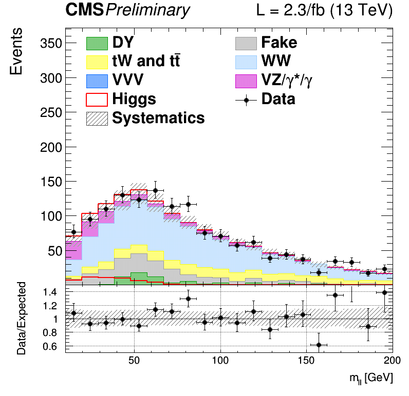
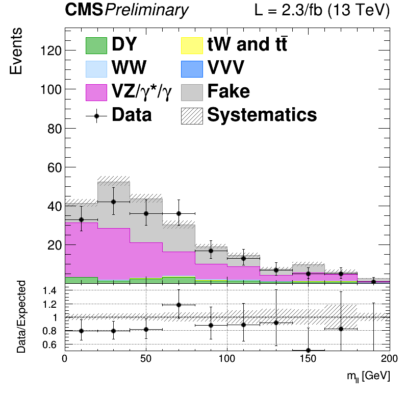
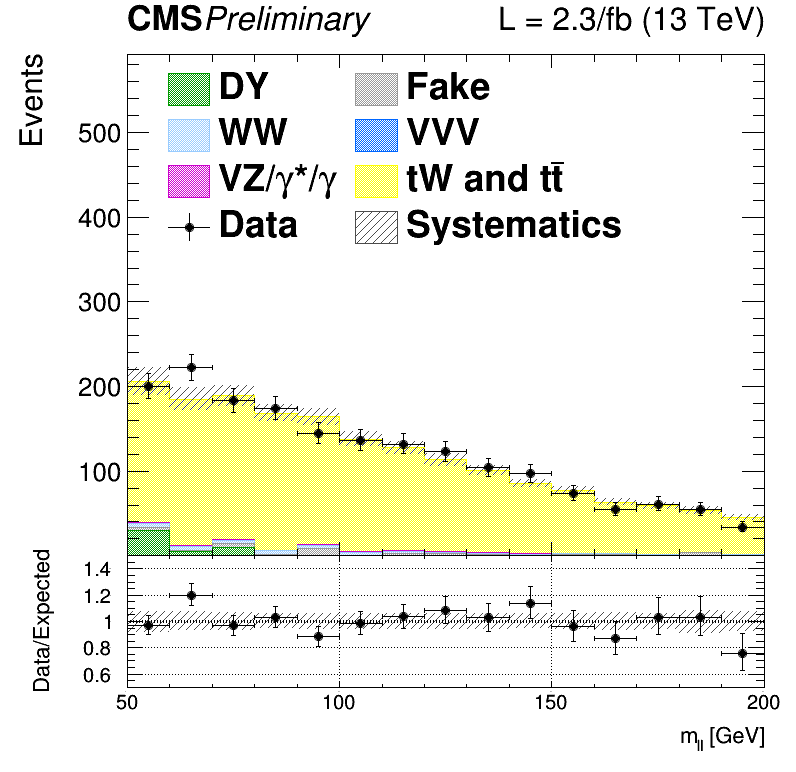
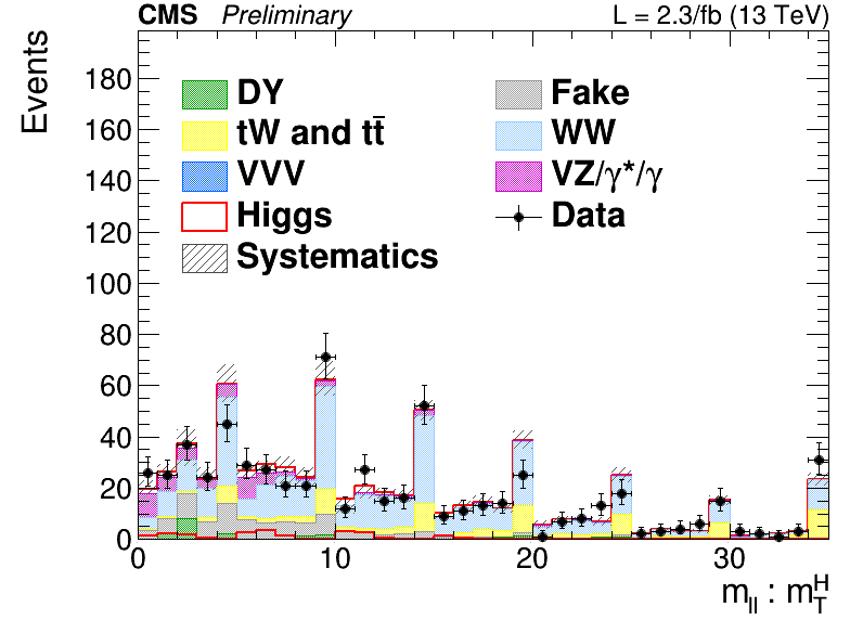
Figure 1-a:
Distributions of ${m_{\ell \ell }}$ (a,c) and ${m_\mathrm {T}^\mathrm {H}}$ (b,d) for events with 0 jet (a,b) and 1 jet (c,d), for the main backgrounds (stacked histograms), and for the expected SM Higgs boson signal with $m_{\mathrm{H}} =$ 125 GeV (superimposed and stacked red histogram) after all selection criteria. The last bin of the histograms includes overflows. Scale factors estimated from data are applied to the jet induced, the Drell-Yan, and top backgrounds. |
png |
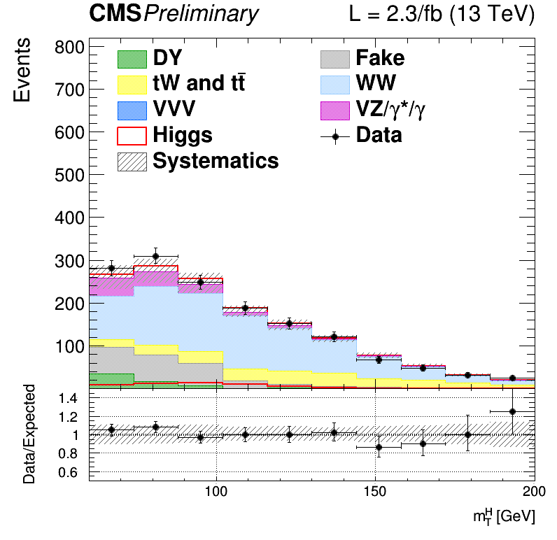
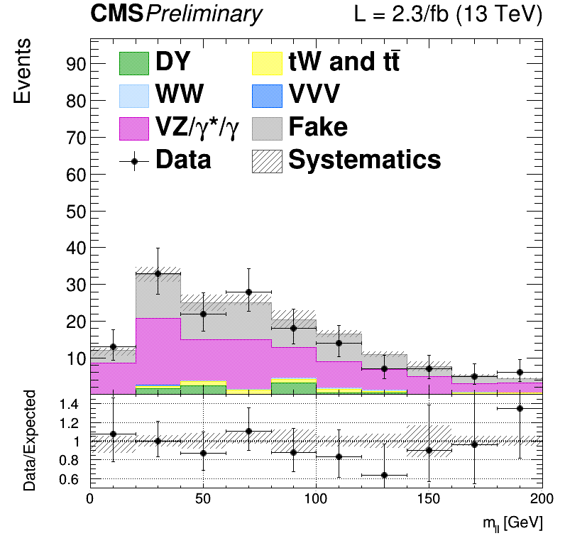
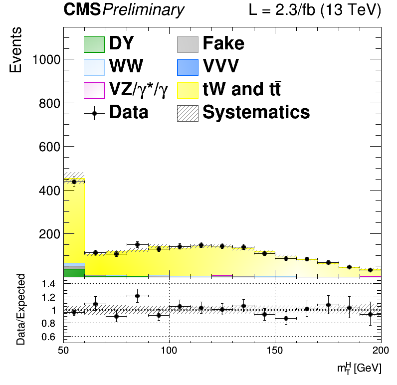
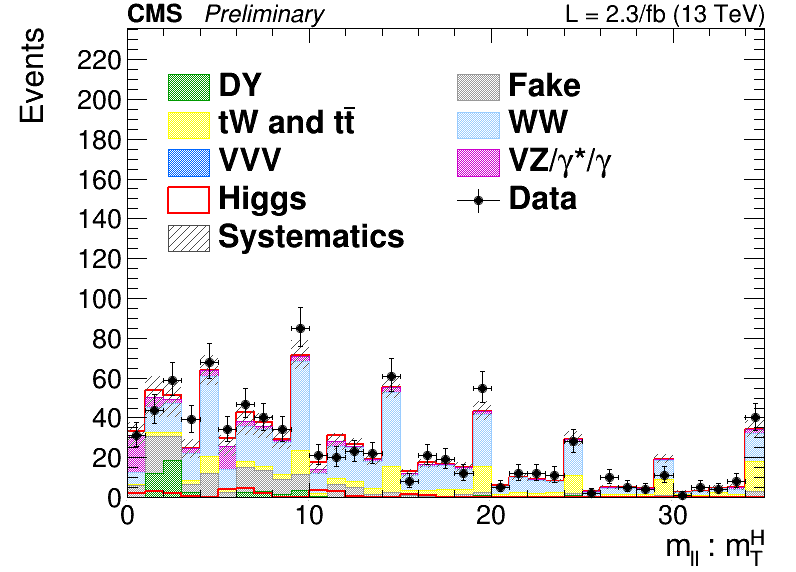
Figure 1-b:
Distributions of ${m_{\ell \ell }}$ (a,c) and ${m_\mathrm {T}^\mathrm {H}}$ (b,d) for events with 0 jet (a,b) and 1 jet (c,d), for the main backgrounds (stacked histograms), and for the expected SM Higgs boson signal with $m_{\mathrm{H}} =$ 125 GeV (superimposed and stacked red histogram) after all selection criteria. The last bin of the histograms includes overflows. Scale factors estimated from data are applied to the jet induced, the Drell-Yan, and top backgrounds. |
png |
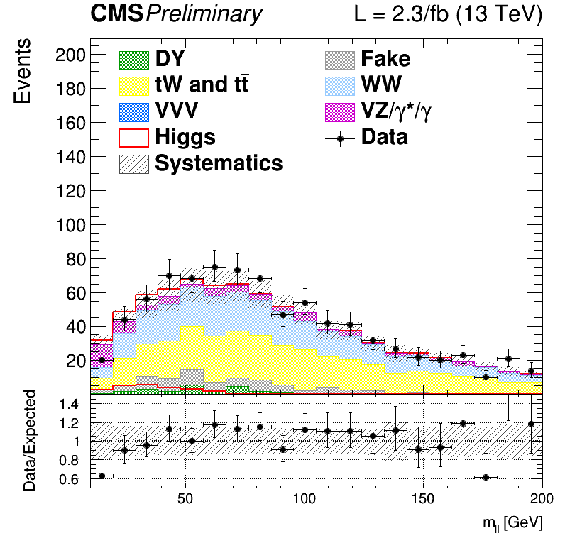
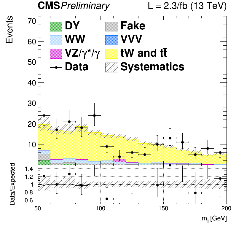
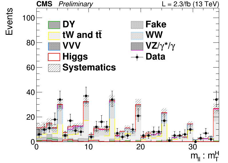
Figure 1-c:
Distributions of ${m_{\ell \ell }}$ (a,c) and ${m_\mathrm {T}^\mathrm {H}}$ (b,d) for events with 0 jet (a,b) and 1 jet (c,d), for the main backgrounds (stacked histograms), and for the expected SM Higgs boson signal with $m_{\mathrm{H}} =$ 125 GeV (superimposed and stacked red histogram) after all selection criteria. The last bin of the histograms includes overflows. Scale factors estimated from data are applied to the jet induced, the Drell-Yan, and top backgrounds. |
png |
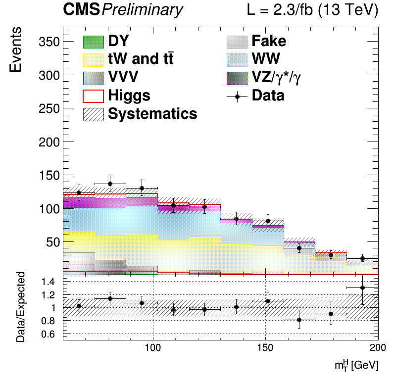
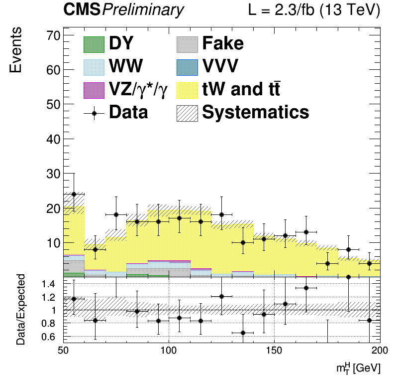
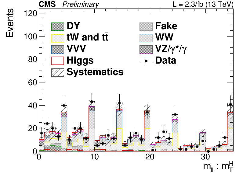
Figure 1-d:
Distributions of ${m_{\ell \ell }}$ (a,c) and ${m_\mathrm {T}^\mathrm {H}}$ (b,d) for events with 0 jet (a,b) and 1 jet (c,d), for the main backgrounds (stacked histograms), and for the expected SM Higgs boson signal with $m_{\mathrm{H}} =$ 125 GeV (superimposed and stacked red histogram) after all selection criteria. The last bin of the histograms includes overflows. Scale factors estimated from data are applied to the jet induced, the Drell-Yan, and top backgrounds. |
png |
Figure 2-a:
Distributions of ${m_{\ell \ell }}$ for events with 0 jet (a) and 1 jet (b) in the same-charge dilepton control region. The global normalisation factor of 0.8 for the jet induced background derived in this control region is applied. The last bin of the histograms includes overflows. |
png |
Figure 2-b:
Distributions of ${m_{\ell \ell }}$ for events with 0 jet (a) and 1 jet (b) in the same-charge dilepton control region. The global normalisation factor of 0.8 for the jet induced background derived in this control region is applied. The last bin of the histograms includes overflows. |
png |
Figure 3-a:
Distributions of ${m_{\ell \ell }}$ (a,c) and ${m_\mathrm {T}^\mathrm {H}}$ (b,d) for events with 0 jet (a,b) and 1 jet (c,d) in top enriched phase space. Scale factors estimated from data are applied. |
png |
Figure 3-b:
Distributions of ${m_{\ell \ell }}$ (a,c) and ${m_\mathrm {T}^\mathrm {H}}$ (b,d) for events with 0 jet (a,b) and 1 jet (c,d) in top enriched phase space. Scale factors estimated from data are applied. |
png |
Figure 3-c:
Distributions of ${m_{\ell \ell }}$ (a,c) and ${m_\mathrm {T}^\mathrm {H}}$ (b,d) for events with 0 jet (a,b) and 1 jet (c,d) in top enriched phase space. Scale factors estimated from data are applied. |
png |
Figure 3-d:
Distributions of ${m_{\ell \ell }}$ (a,c) and ${m_\mathrm {T}^\mathrm {H}}$ (b,d) for events with 0 jet (a,b) and 1 jet (c,d) in top enriched phase space. Scale factors estimated from data are applied. |
png |
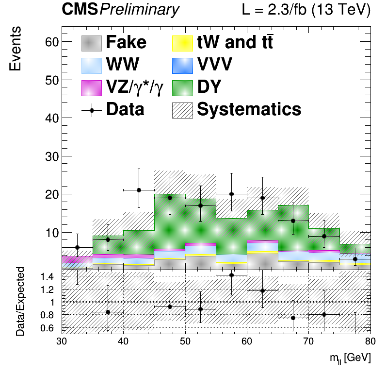
Figure 4-a:
Distributions of ${m_{\ell \ell }}$ for events with 0 jet (a) and 1 jet (b) in the DY$\rightarrow \tau \tau $ ${m_\mathrm {T}^\mathrm {H}} < $ 60 GeV and 30 GeV $< {m_{\ell \ell }} <$ 80 GeV control region. Scale factors estimated from the normalization difference to the data are applied. |
png |
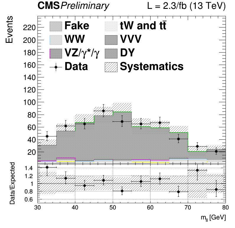
Figure 4-b:
Distributions of ${m_{\ell \ell }}$ for events with 0 jet (a) and 1 jet (b) in the DY$\rightarrow \tau \tau $ ${m_\mathrm {T}^\mathrm {H}} < $ 60 GeV and 30 GeV $< {m_{\ell \ell }} <$ 80 GeV control region. Scale factors estimated from the normalization difference to the data are applied. |
png |
Figure 5-a:
Bi-dimensional distributions of the ${m_{\ell \ell }}$ and ${m_\mathrm {T}^\mathrm {H}}$ templates in the 0-jet (a,b) and 1-jet (c,d) and $\mu $e (a,c) and e$\mu $ (b,d) categories after the WW level selection. The bi-dimensional templates ranges are 10 $ < {m_{\ell \ell }} < $ 110 GeV and 0 $ < {m_\mathrm {T}^\mathrm {H}} < $ 200 GeV with 5 bins in ${m_{\ell \ell }}$ and 10 bins in ${m_\mathrm {T}^\mathrm {H}} $. The distributions are unrolled to one dimensional histograms such that that identical values of ${m_\mathrm {T}^\mathrm {H}}$ are in adjacent bins. The background and signal contributions are normalized according to their pre-fit values except that scale factors estimated from data are applied to the jet induced, the Drell-Yan, and top backgrounds. |
png |
Figure 5-b:
Bi-dimensional distributions of the ${m_{\ell \ell }}$ and ${m_\mathrm {T}^\mathrm {H}}$ templates in the 0-jet (a,b) and 1-jet (c,d) and $\mu $e (a,c) and e$\mu $ (b,d) categories after the WW level selection. The bi-dimensional templates ranges are 10 $ < {m_{\ell \ell }} < $ 110 GeV and 0 $ < {m_\mathrm {T}^\mathrm {H}} < $ 200 GeV with 5 bins in ${m_{\ell \ell }}$ and 10 bins in ${m_\mathrm {T}^\mathrm {H}} $. The distributions are unrolled to one dimensional histograms such that that identical values of ${m_\mathrm {T}^\mathrm {H}}$ are in adjacent bins. The background and signal contributions are normalized according to their pre-fit values except that scale factors estimated from data are applied to the jet induced, the Drell-Yan, and top backgrounds. |
png |
Figure 5-c:
Bi-dimensional distributions of the ${m_{\ell \ell }}$ and ${m_\mathrm {T}^\mathrm {H}}$ templates in the 0-jet (a,b) and 1-jet (c,d) and $\mu $e (a,c) and e$\mu $ (b,d) categories after the WW level selection. The bi-dimensional templates ranges are 10 $ < {m_{\ell \ell }} < $ 110 GeV and 0 $ < {m_\mathrm {T}^\mathrm {H}} < $ 200 GeV with 5 bins in ${m_{\ell \ell }}$ and 10 bins in ${m_\mathrm {T}^\mathrm {H}} $. The distributions are unrolled to one dimensional histograms such that that identical values of ${m_\mathrm {T}^\mathrm {H}}$ are in adjacent bins. The background and signal contributions are normalized according to their pre-fit values except that scale factors estimated from data are applied to the jet induced, the Drell-Yan, and top backgrounds. |
png |
Figure 5-d:
Bi-dimensional distributions of the ${m_{\ell \ell }}$ and ${m_\mathrm {T}^\mathrm {H}}$ templates in the 0-jet (a,b) and 1-jet (c,d) and $\mu $e (a,c) and e$\mu $ (b,d) categories after the WW level selection. The bi-dimensional templates ranges are 10 $ < {m_{\ell \ell }} < $ 110 GeV and 0 $ < {m_\mathrm {T}^\mathrm {H}} < $ 200 GeV with 5 bins in ${m_{\ell \ell }}$ and 10 bins in ${m_\mathrm {T}^\mathrm {H}} $. The distributions are unrolled to one dimensional histograms such that that identical values of ${m_\mathrm {T}^\mathrm {H}}$ are in adjacent bins. The background and signal contributions are normalized according to their pre-fit values except that scale factors estimated from data are applied to the jet induced, the Drell-Yan, and top backgrounds. |
| Summary |
| A measurement of the SM Higgs boson decaying to WW in pp collisions at $\sqrt{s} =$ 13 TeV is performed by the CMS experiment using a data sample corresponding to an integrated luminosity of 2.3 fb$^{-1}$. The $\mathrm{W^+W^-}$ candidates are selected in events with an oppositely charged $\mathrm{e}\mu$ pair and large missing transverse momentum in association with up to one additional jet. The observed (expected) significance for a SM Higgs boson with a mass of 125 GeV is 0.7$\sigma$ (2.0$\sigma$), corresponding to an observed cross section times branching ratio of 0.3 $\pm$ 0.5 times the standard model prediction. |
| References | ||||
| 1 | F. Englert and R. Brout | Broken Symmetry and the Mass of Gauge Vector Mesons | PRL 13 (1964) 321 | |
| 2 | P. W. Higgs | Broken symmetries, massless particles and gauge fields | PL12 (1964) 132 | |
| 3 | P. W. Higgs | Broken Symmetries and the Masses of Gauge Bosons | PRL 13 (1964) 508 | |
| 4 | G. S. Guralnik, C. R. Hagen, and T. W. B. Kibble | Global conservation laws and massless particles | PRL 13 (1964) 585 | |
| 5 | P. W. Higgs | Spontaneous symmetry breakdown without massless bosons | PR145 (1966) 1156 | |
| 6 | T. W. B. Kibble | Symmetry breaking in non-Abelian gauge theories | PR155 (1967) 1554 | |
| 7 | ATLAS Collaboration | Observation of a new particle in the search for the Standard Model Higgs boson with the ATLAS detector at the LHC | PLB 716 (2012) 1 | 1207.7214 |
| 8 | CMS Collaboration | Observation of a new boson at a mass of 125 GeV with the CMS experiment at the LHC | PLB 716 (2012) 30 | CMS-HIG-12-028 1207.7235 |
| 9 | ATLAS Collaboration | Measurements of the Higgs boson production and decay rates and coupling strengths using pp collision data at $ \sqrt{s}=7 $ and 8 TeV in the ATLAS experiment | EPJC76 (2016), no. 1, 6 | 1507.04548 |
| 10 | ATLAS Collaboration | Evidence for the spin-0 nature of the Higgs boson using ATLAS data | PLB726 (2013) 120--144 | 1307.1432 |
| 11 | CMS Collaboration | Precise determination of the mass of the Higgs boson and tests of compatibility of its couplings with the standard model predictions using proton collisions at 7 and 8 $ \,\text {TeV} $ | EPJC75 (2015), no. 5, 212 | CMS-HIG-14-009 1412.8662 |
| 12 | CMS Collaboration | Constraints on the spin-parity and anomalous HVV couplings of the Higgs boson in proton collisions at 7 and 8 TeV | PRD92 (2015), no. 1, 012004 | CMS-HIG-14-018 1411.3441 |
| 13 | ATLAS and CMS | Combined Measurement of the Higgs Boson Mass in $ pp $ Collisions at $ \sqrt{s}=7 $ and 8 TeV with the ATLAS and CMS Experiments | PRL 114 (2015) 191803 | 1503.07589 |
| 14 | ATLAS and CMS | Measurements of the Higgs boson production and decay rates and constraints on its couplings from a combined ATLAS and CMS analysis of the LHC pp collision data at $ \sqrt{s} $ = 7 and 8 TeV | Technical Report CMS-PAS-HIG-15-002, CERN, Geneva | |
| 15 | CMS Collaboration | Measurement of Higgs boson production and properties in the WW decay channel with leptonic final states | JHEP 01 (2014) 096 | CMS-HIG-13-023 1312.1129 |
| 16 | CMS Collaboration | The CMS experiment at the CERN LHC | JINST 3 (2008) S08004 | |
| 17 | P. Nason | A New method for combining NLO QCD with shower Monte Carlo algorithms | JHEP 11 (2004) 040 | hep-ph/0409146 |
| 18 | S. Frixione, P. Nason, and C. Oleari | Matching NLO QCD computations with Parton Shower simulations: the POWHEG method | JHEP 11 (2007) 070 | 0709.2092 |
| 19 | S. Alioli, P. Nason, C. Oleari, and E. Re | A general framework for implementing NLO calculations in shower Monte Carlo programs: the POWHEG BOX | JHEP 06 (2010) 043 | 1002.2581 |
| 20 | S. Alioli, P. Nason, C. Oleari, and E. Re | NLO Higgs boson production via gluon fusion matched with shower in POWHEG | JHEP 04 (2009) 002 | 0812.0578 |
| 21 | P. Nason and C. Oleari | NLO Higgs boson production via vector-boson fusion matched with shower in POWHEG | JHEP 02 (2010) 037 | 0911.5299 |
| 22 | S. Bolognesi, Y. Gao, A. Gritsan et al. | |||
| 23 | G. Luisoni, P. Nason, C. Oleari, and F. Tramontano | $ HW^{\pm} $/HZ + 0 and 1 jet at NLO with the POWHEG BOX interfaced to GoSam and their merging within MiNLO | JHEP 10 (2013) 083 | 1306.2542 |
| 24 | T. Sjostrand, S. Mrenna, and P. Z. Skands | A Brief Introduction to PYTHIA 8.1 | CPC 178 (2008) 852--867 | 0710.3820 |
|
|
Compact Muon Solenoid LHC, CERN |
|

|

|

|

|

|