

Compact Muon Solenoid
LHC, CERN
| CMS-PAS-HIG-16-020 | ||
| Updated measurements of Higgs boson production in the diphoton decay channel at $\sqrt{s}=$ 13 TeV in pp collisions at CMS. | ||
| CMS Collaboration | ||
| August 2016 | ||
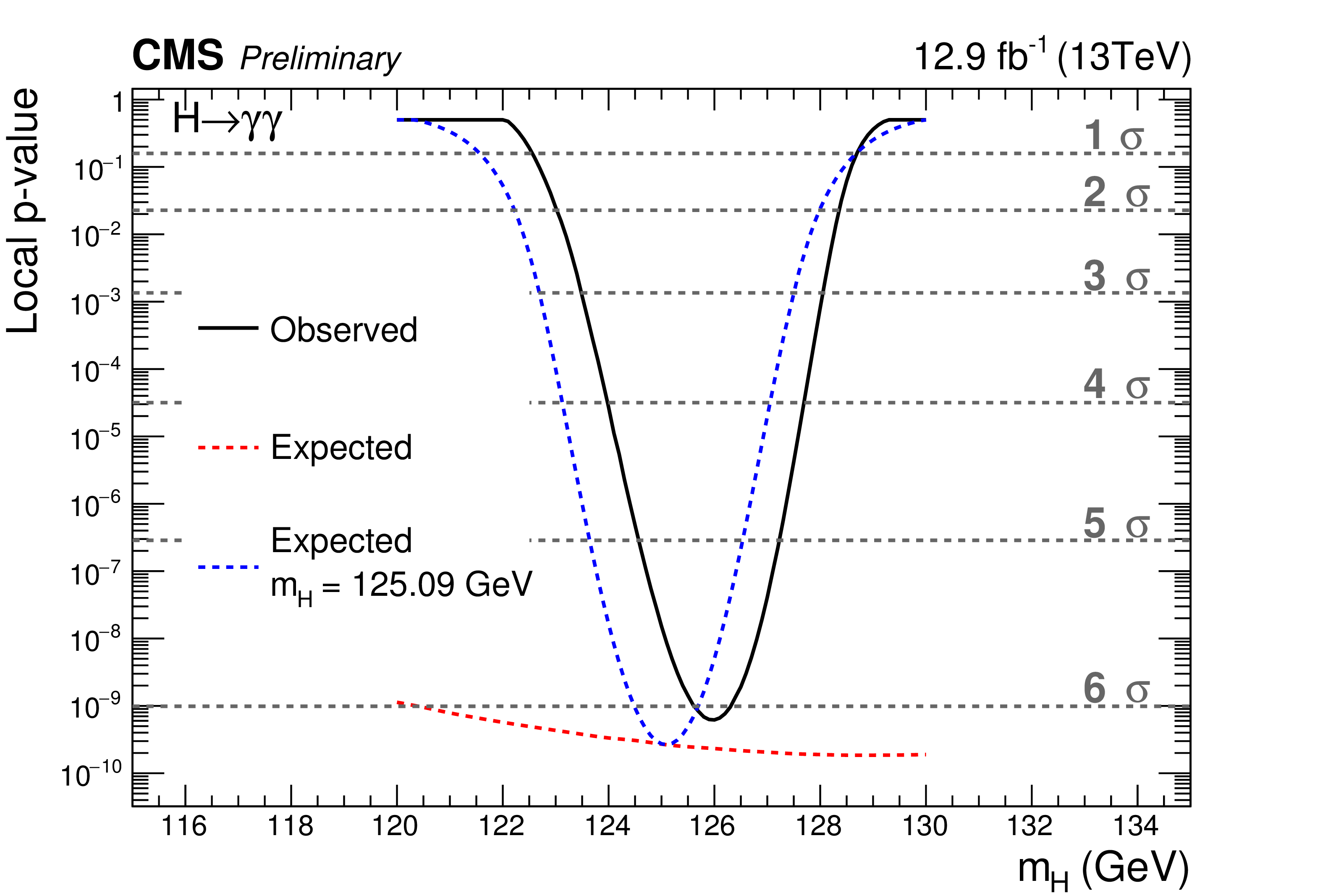
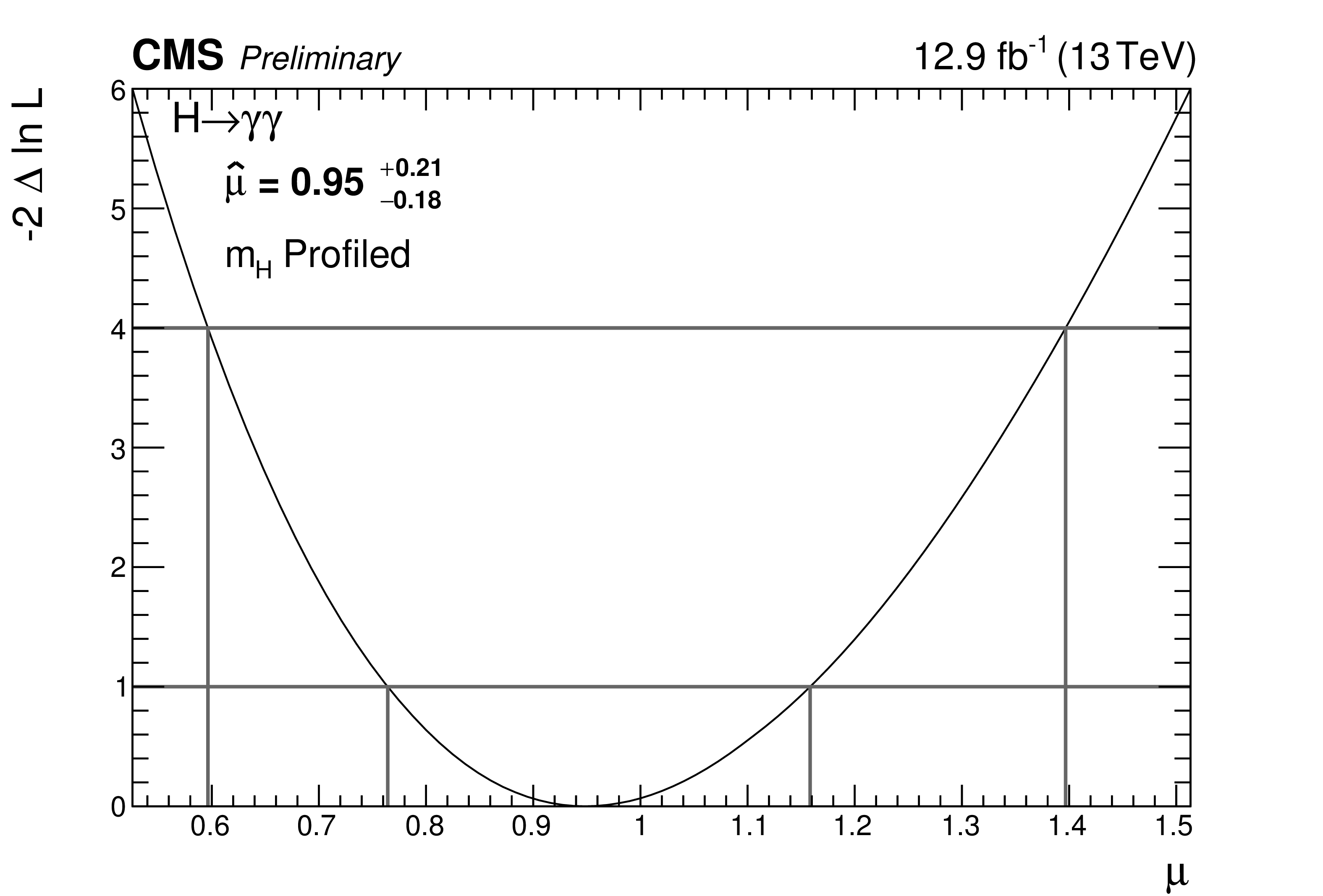
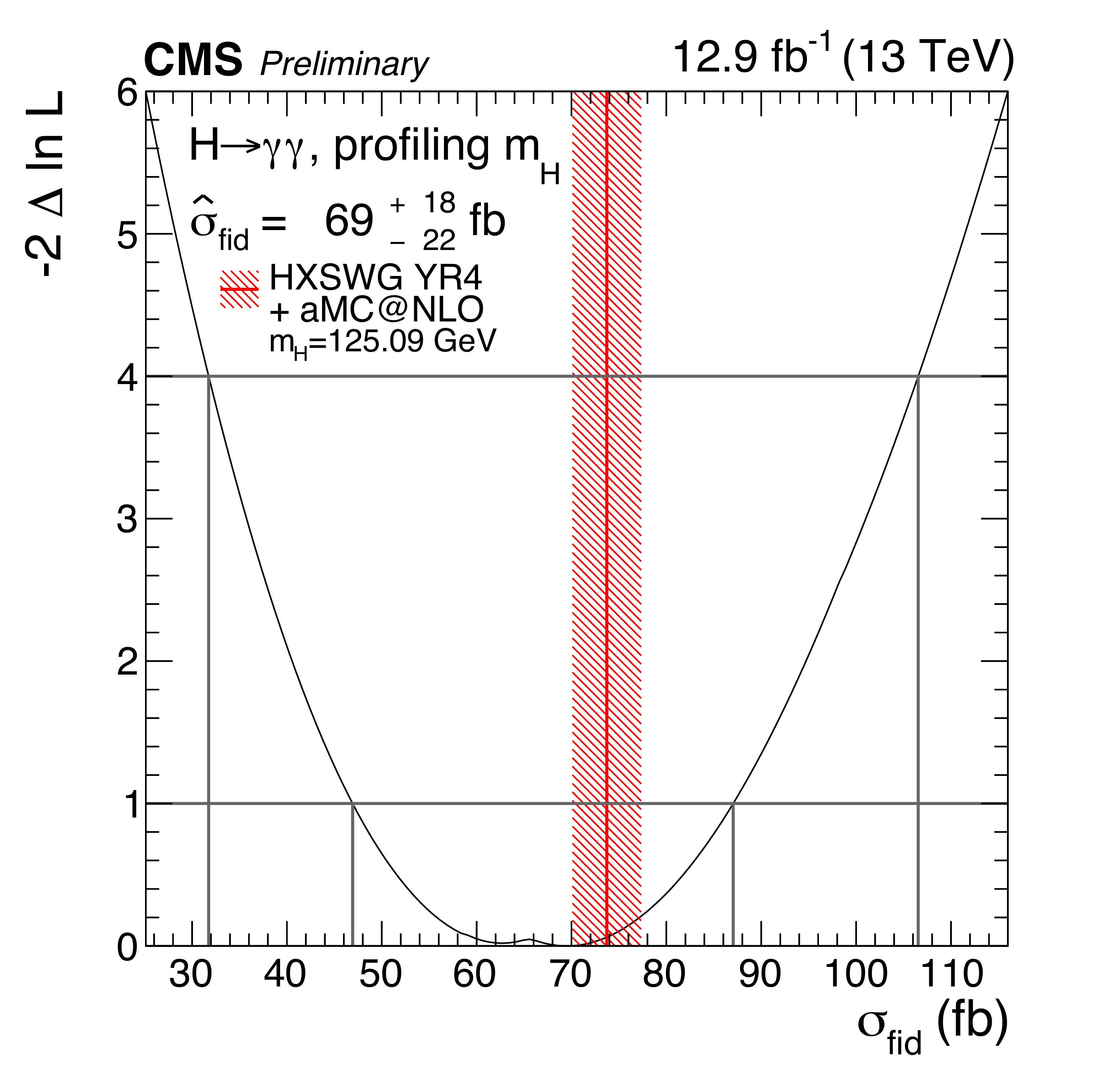
| Abstract: An observation of the Higgs boson production for the two photon decay channel with the 2016 LHC Run-2 data is described. The analysis is performed using the dataset recorded by the CMS experiment at the LHC from pp collisions at centre-of-mass energy of 13 TeV corresponding to an integrated luminosity of 12.9 fb$^{-1}$. The observed significance for the standard model Higgs boson at the Run 1 ATLAS+CMS combined $m_{\mathrm{H}} =$ 125.09 GeV is 5.6$ \sigma$, where 6.2$ \sigma$ is expected. A maximum significance of 6.1$ \sigma$ is observed at 126.0 GeV. The best-fit signal strength relative to the standard model prediction is 0.95 $\pm$ 0.20 = 0.95 $\pm$ 0.17 (stat) $^{+0.10}_{-0.07}$ (syst) $^{+0.08}_{-0.05}$ (theo) when the mass parameter is profiled in the fit, and 0.91 $\pm$ 0.20 = 0.91 $\pm$ 0.17 (stat) $^{+0.09}_{-0.07}$ (syst) $^{+0.08}_{-0.05}$ (theo) when it is fixed to $m_{\mathrm{H}} =$ 125.09 GeV. The fiducial cross section is measured to be $\hat{\sigma}_{fid} =$ 69 $^{+18}_{-22}$ fb = 69 $^{+16}_{-22}$ (stat) $^{+8} _{-6}$ (syst) fb, where the standard model theoretical prediction is 73.8 $\pm$ 3.8 fb. | ||
| Links: CDS record (PDF) ; inSPIRE record ; CADI line (restricted) ; | ||
| Figures | |

png pdf |
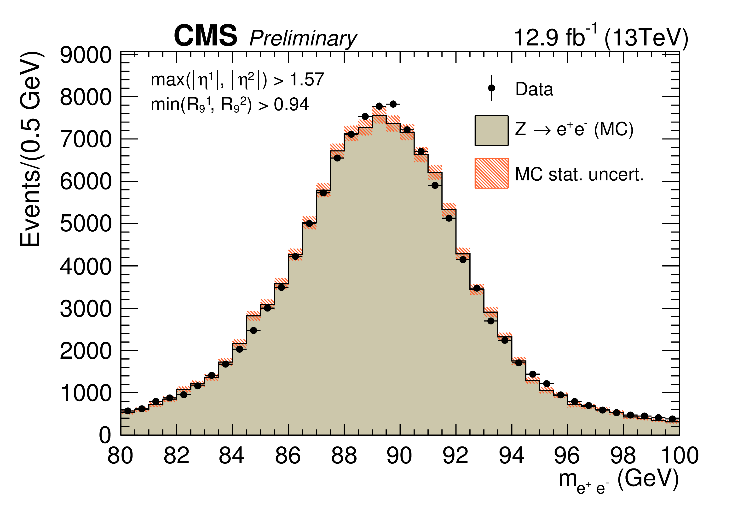
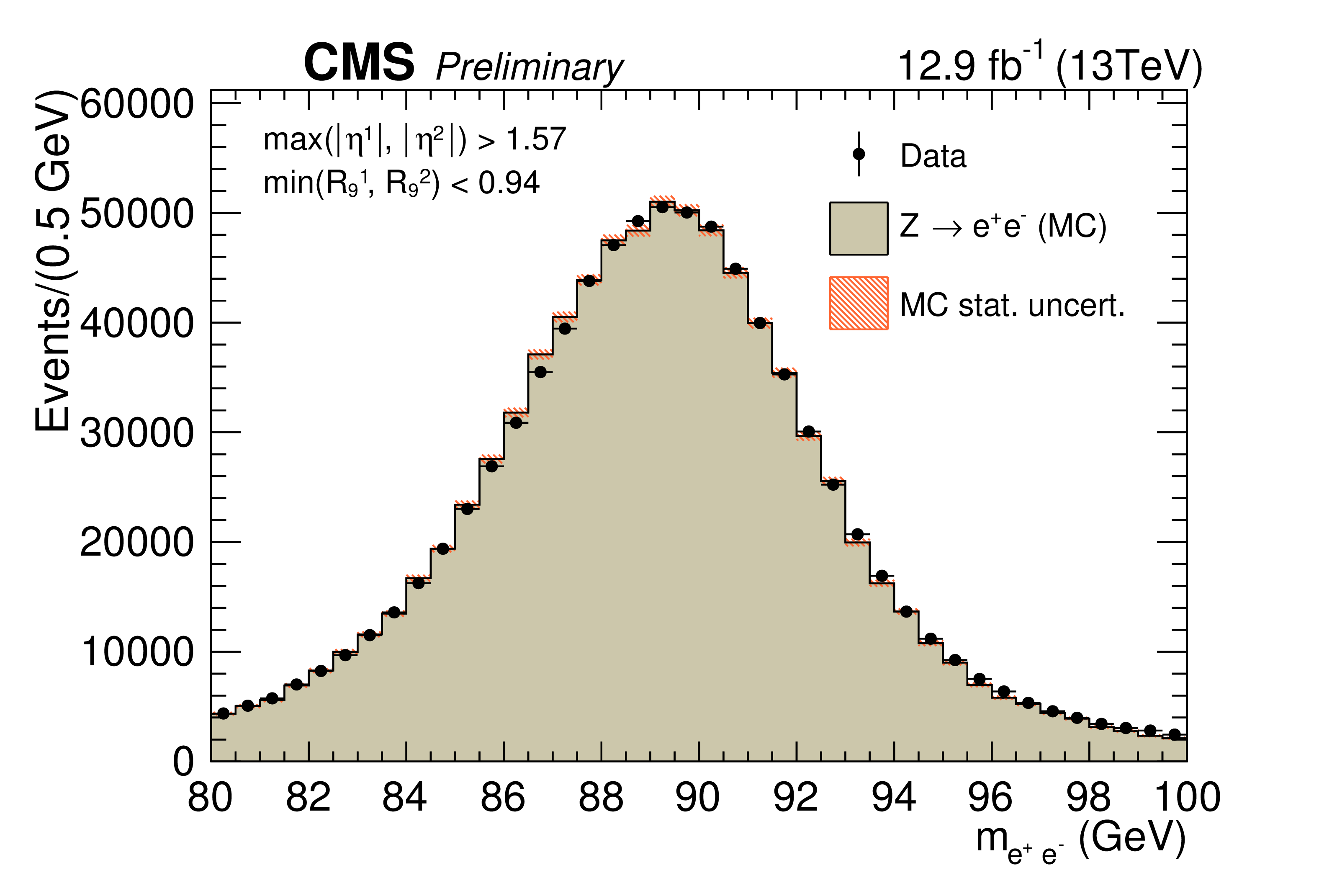
Figure 1-a:
Comparison of the dielectron invariant mass distributions in data and simulation for Z$\rightarrow $ e$^{+}$e$^{-}$ events where electrons are reconstructed as photons. The events are split into categories according to the $\eta $ and $ {R_\mathrm {9}}$ of the electrons. The simulated distribution is normalized to the integral of the data distribution in the range 87 GeV $ < m_{e^{+}e^{-}} < $ 93 GeV. |

png pdf |
Figure 1-b:
Comparison of the dielectron invariant mass distributions in data and simulation for Z$\rightarrow $ e$^{+}$e$^{-}$ events where electrons are reconstructed as photons. The events are split into categories according to the $\eta $ and $ {R_\mathrm {9}}$ of the electrons. The simulated distribution is normalized to the integral of the data distribution in the range 87 GeV $ < m_{e^{+}e^{-}} < $ 93 GeV. |
png pdf |
Figure 1-c:
Comparison of the dielectron invariant mass distributions in data and simulation for Z$\rightarrow $ e$^{+}$e$^{-}$ events where electrons are reconstructed as photons. The events are split into categories according to the $\eta $ and $ {R_\mathrm {9}}$ of the electrons. The simulated distribution is normalized to the integral of the data distribution in the range 87 GeV $ < m_{e^{+}e^{-}} < $ 93 GeV. |
png pdf |
Figure 1-d:
Comparison of the dielectron invariant mass distributions in data and simulation for Z$\rightarrow $ e$^{+}$e$^{-}$ events where electrons are reconstructed as photons. The events are split into categories according to the $\eta $ and $ {R_\mathrm {9}}$ of the electrons. The simulated distribution is normalized to the integral of the data distribution in the range 87 GeV $ < m_{e^{+}e^{-}} < $ 93 GeV. |

png pdf |
Figure 2:
Comparison of the true vertex identification efficiency and the average estimated vertex probability as a function of the reconstructed diphoton ${p_{\mathrm {T}}} $ in simulated H$\to \gamma \gamma $ events with $ {m_{\mathrm {H}} }=$ 125 GeV. Events are weighted according to the cross-sections of the different production modes and to match distributions of pileup and location of primary vertices in data. |
png pdf |
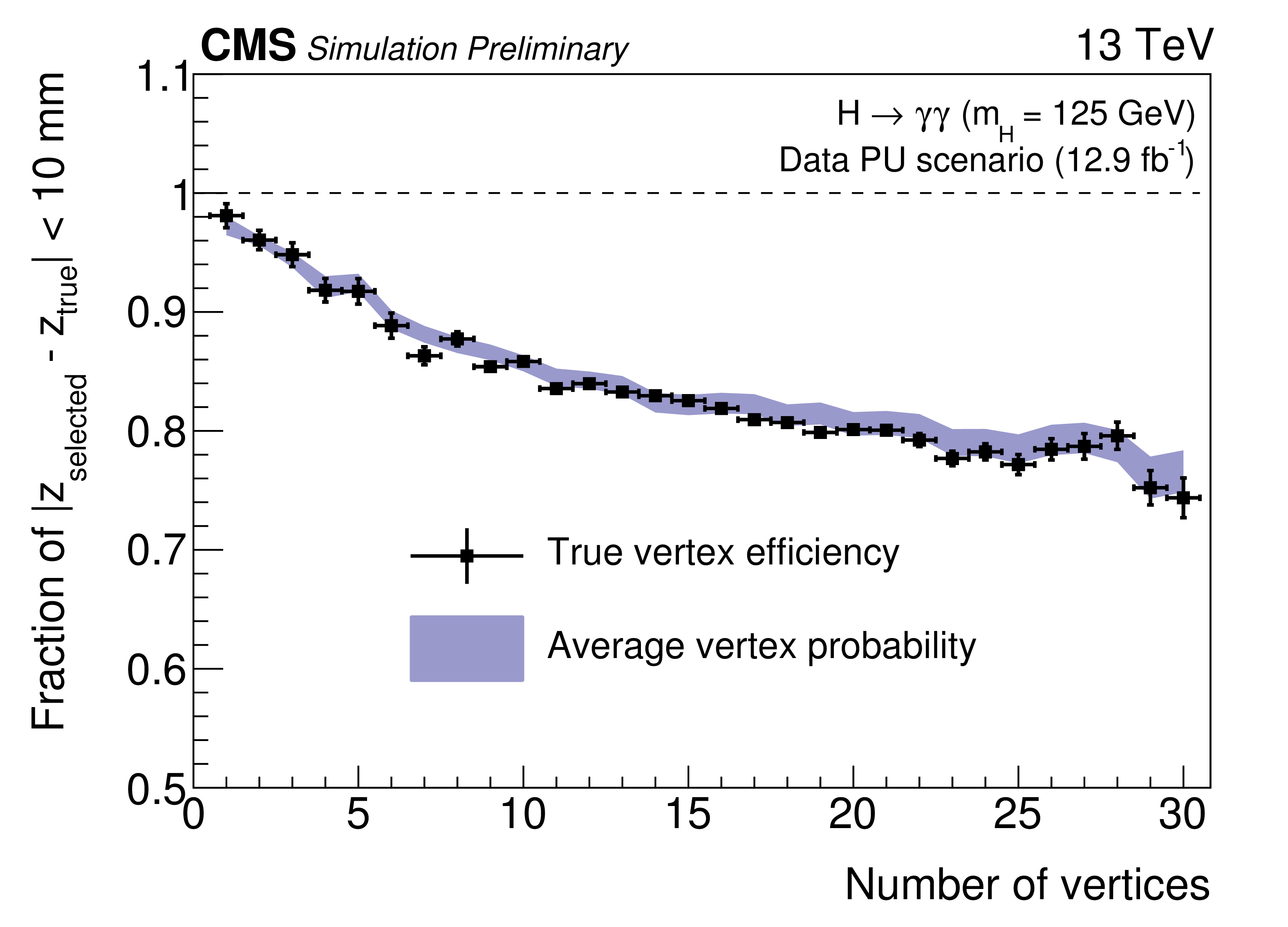
Figure 3:
Comparison of the true vertex identification efficiency and the average estimated vertex probability as a function of the number of primary vertices in simulated H$\to \gamma \gamma $ events with $ {m_{\mathrm {H}} }=$ 125 GeV. Events are weighted according to the cross-sections of the different production modes and to match distributions of pileup and location of primary vertices in data. |
png pdf |
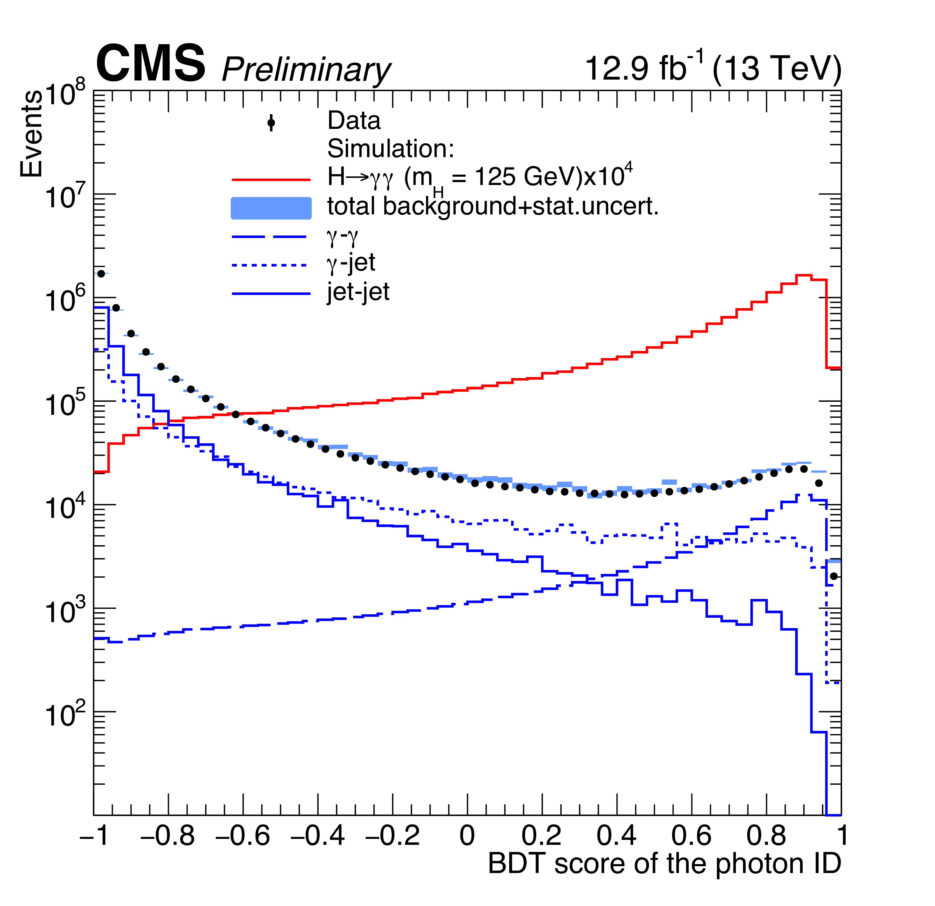
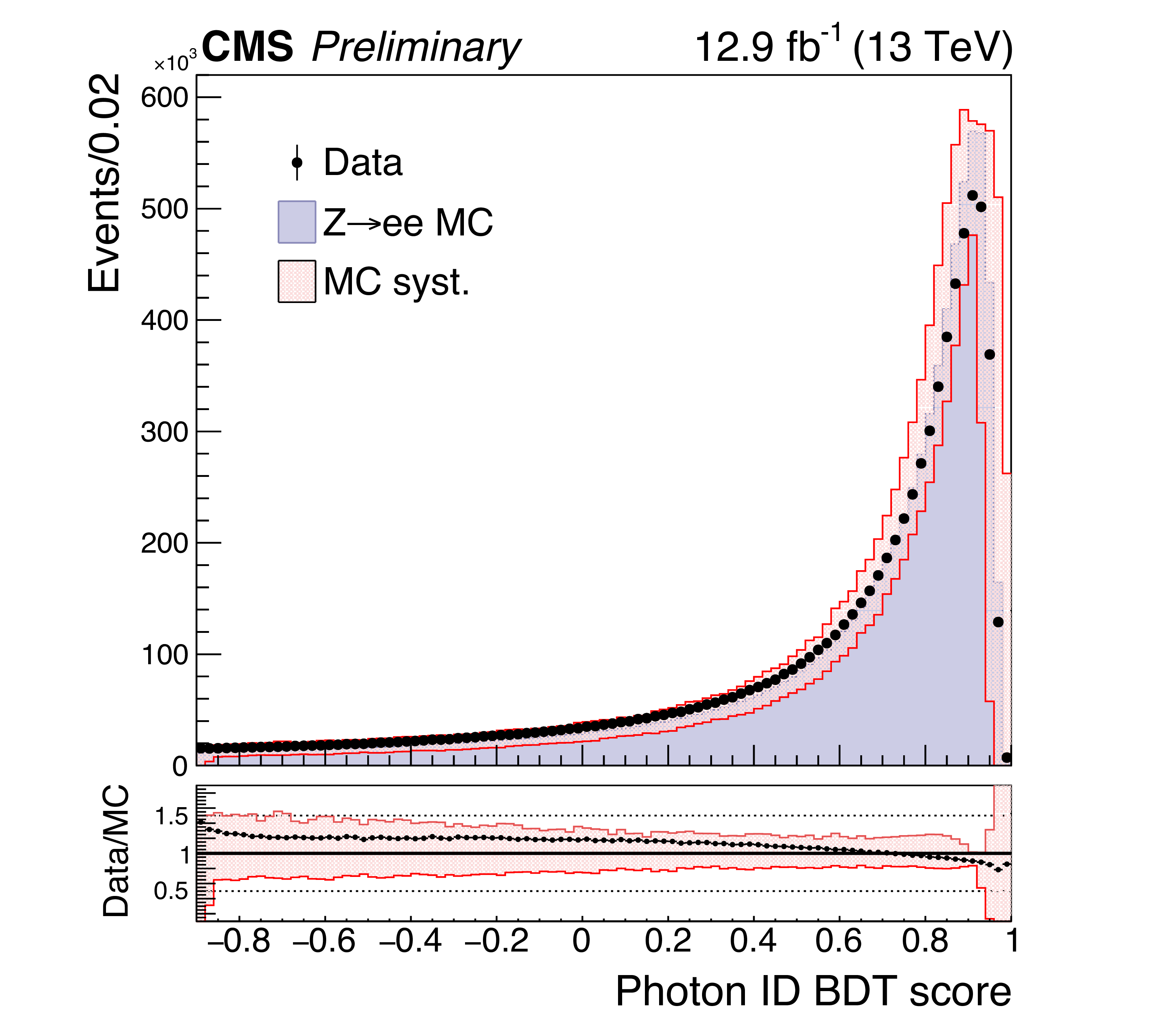
Figure 4-a:
(a) $\text {BDT}_{\gamma \text { ID}}$ score of the lower-scoring photon of diphoton pairs with an invariant mass in the range 100 $ < m_{\gamma \gamma } < $ 180 GeV, for events passing the preselection in the 13TeV dataset (points), and for simulated background events (blue histogram). Histograms are also shown for different components of the simulated background, in which there are either two, one, or zero prompt candidate photons. The sum of all background distributions, generated at leading order, is scaled up to data. The red histogram corresponds to simulated Higgs boson signal events. (b) $\text {BDT}_{\gamma \text { ID}}$ score for Z$\rightarrow $ e$^{+}$e$^{-}$ events in data and simulation, where the electrons are reconstructed as photons. The systematic uncertainty applied to the shape from simulation (hashed region) is also shown. |
png pdf |
Figure 4-b:
(a) $\text {BDT}_{\gamma \text { ID}}$ score of the lower-scoring photon of diphoton pairs with an invariant mass in the range 100 $ < m_{\gamma \gamma } < $ 180 GeV, for events passing the preselection in the 13TeV dataset (points), and for simulated background events (blue histogram). Histograms are also shown for different components of the simulated background, in which there are either two, one, or zero prompt candidate photons. The sum of all background distributions, generated at leading order, is scaled up to data. The red histogram corresponds to simulated Higgs boson signal events. (b) $\text {BDT}_{\gamma \text { ID}}$ score for Z$\rightarrow $ e$^{+}$e$^{-}$ events in data and simulation, where the electrons are reconstructed as photons. The systematic uncertainty applied to the shape from simulation (hashed region) is also shown. |
png pdf |
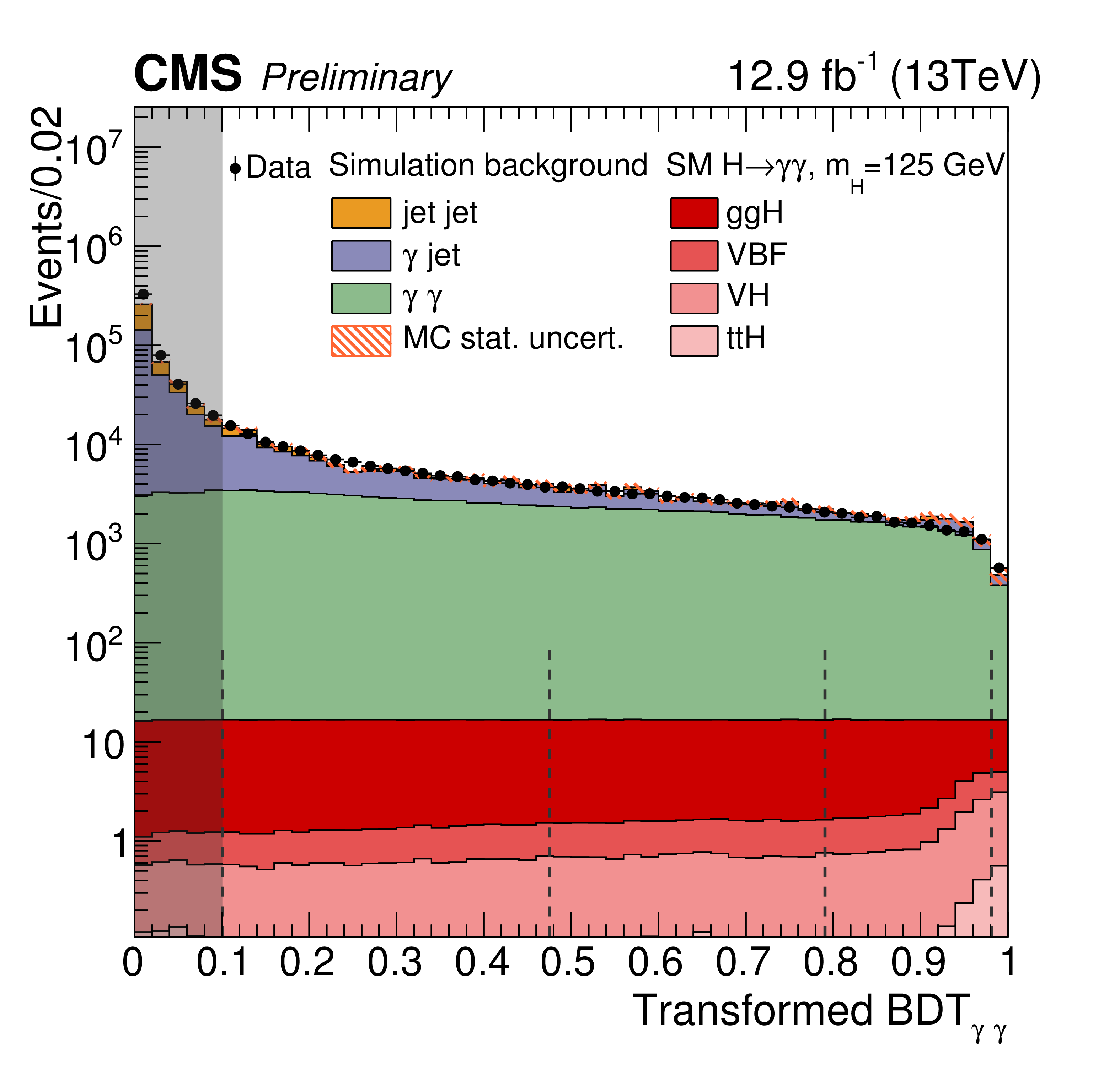
Figure 5-a:
(a) Transformed $\text {BDT}_{\gamma \gamma }$ classifier score in data (black points) and simulation (stacked histograms) for events in the region 100 $ < m_{\gamma \gamma } < $ 180 GeV. (b) Transformed $\text {BDT}_{\gamma \gamma }$ classifier score for Z$\rightarrow $ e$^{+}$e$^{-}$ events, where electrons are reconstructed as photons, in data (black points) and simulation (filled histogram). The hashed region represents the systematic uncertainty resulting from the combination of the uncertainties on the $\text {BDT}_{\gamma \text { ID}}$ and the photon energy resolution. The gray bands represent events rejected in the analysis. |
png pdf |
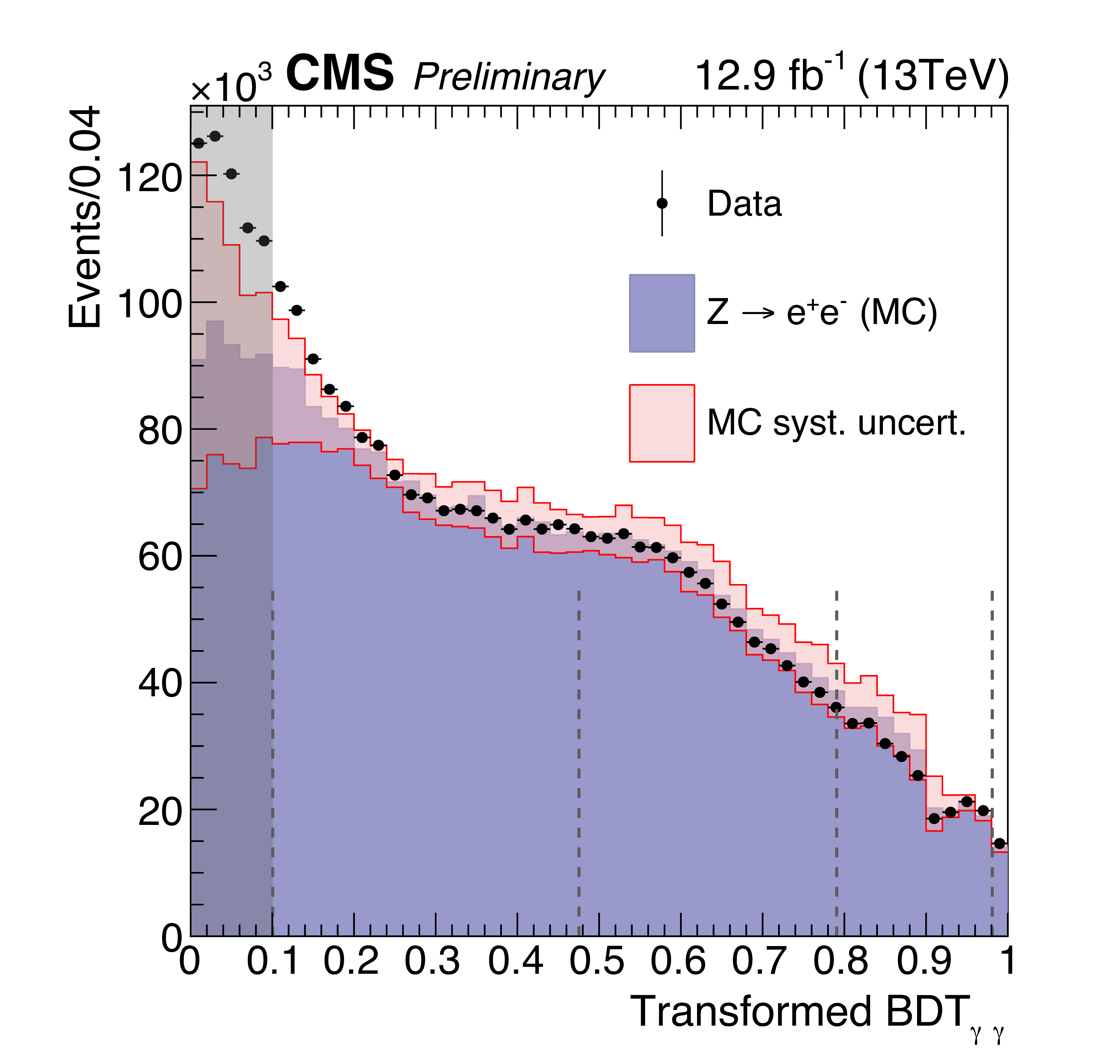
Figure 5-b:
(a) Transformed $\text {BDT}_{\gamma \gamma }$ classifier score in data (black points) and simulation (stacked histograms) for events in the region 100 $ < m_{\gamma \gamma } < $ 180 GeV. (b) Transformed $\text {BDT}_{\gamma \gamma }$ classifier score for Z$\rightarrow $ e$^{+}$e$^{-}$ events, where electrons are reconstructed as photons, in data (black points) and simulation (filled histogram). The hashed region represents the systematic uncertainty resulting from the combination of the uncertainties on the $\text {BDT}_{\gamma \text { ID}}$ and the photon energy resolution. The gray bands represent events rejected in the analysis. |
png pdf |
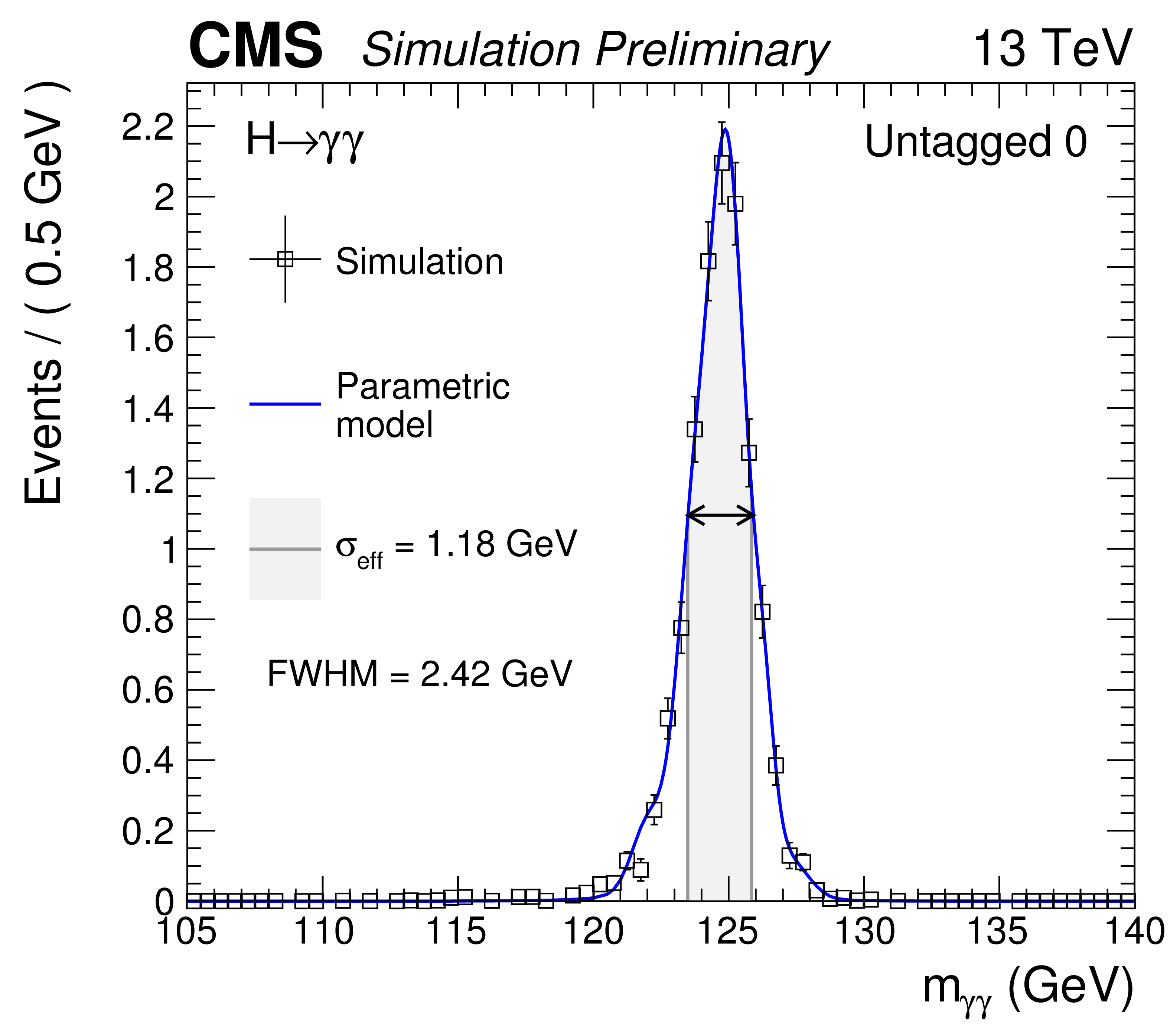
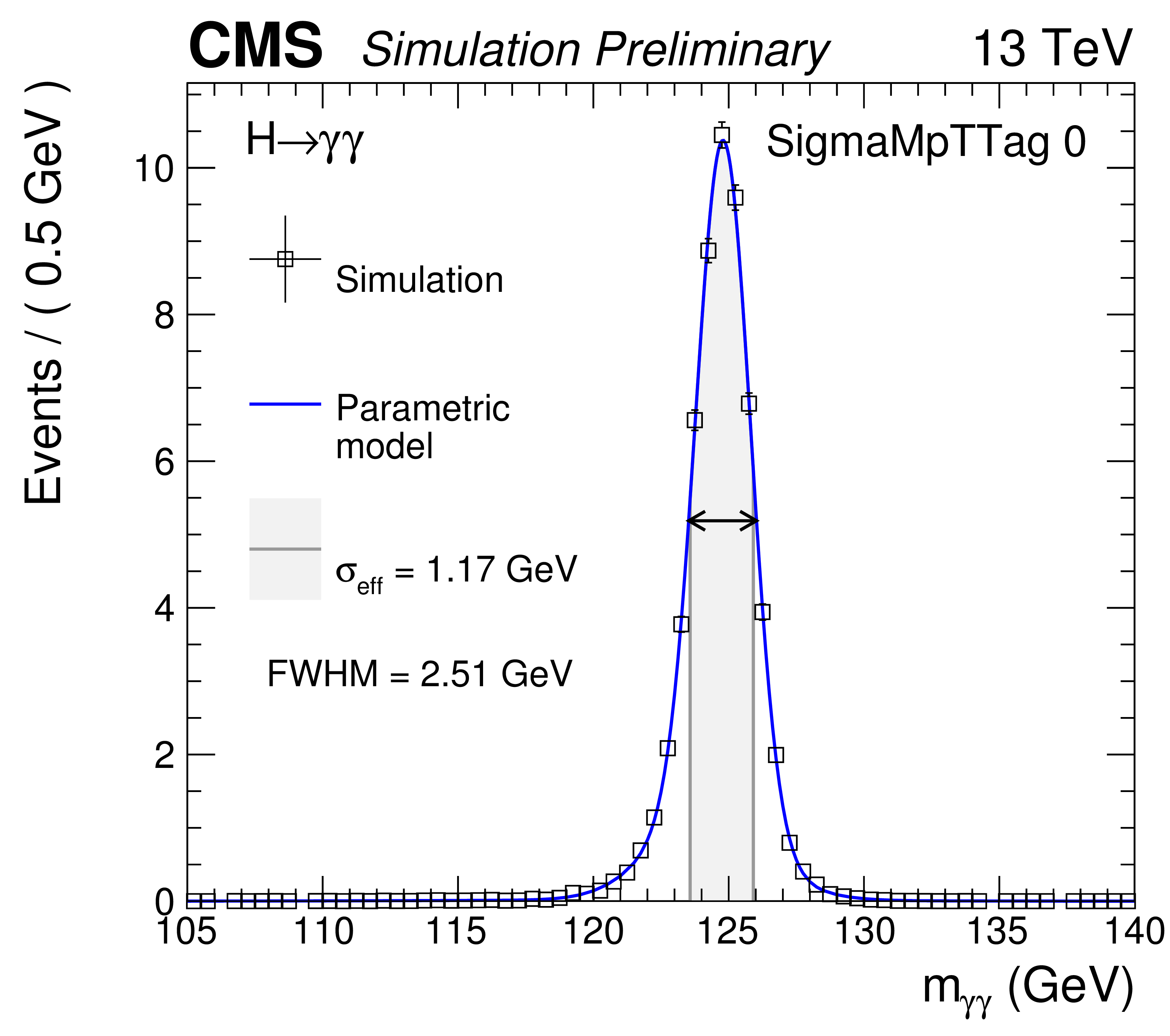
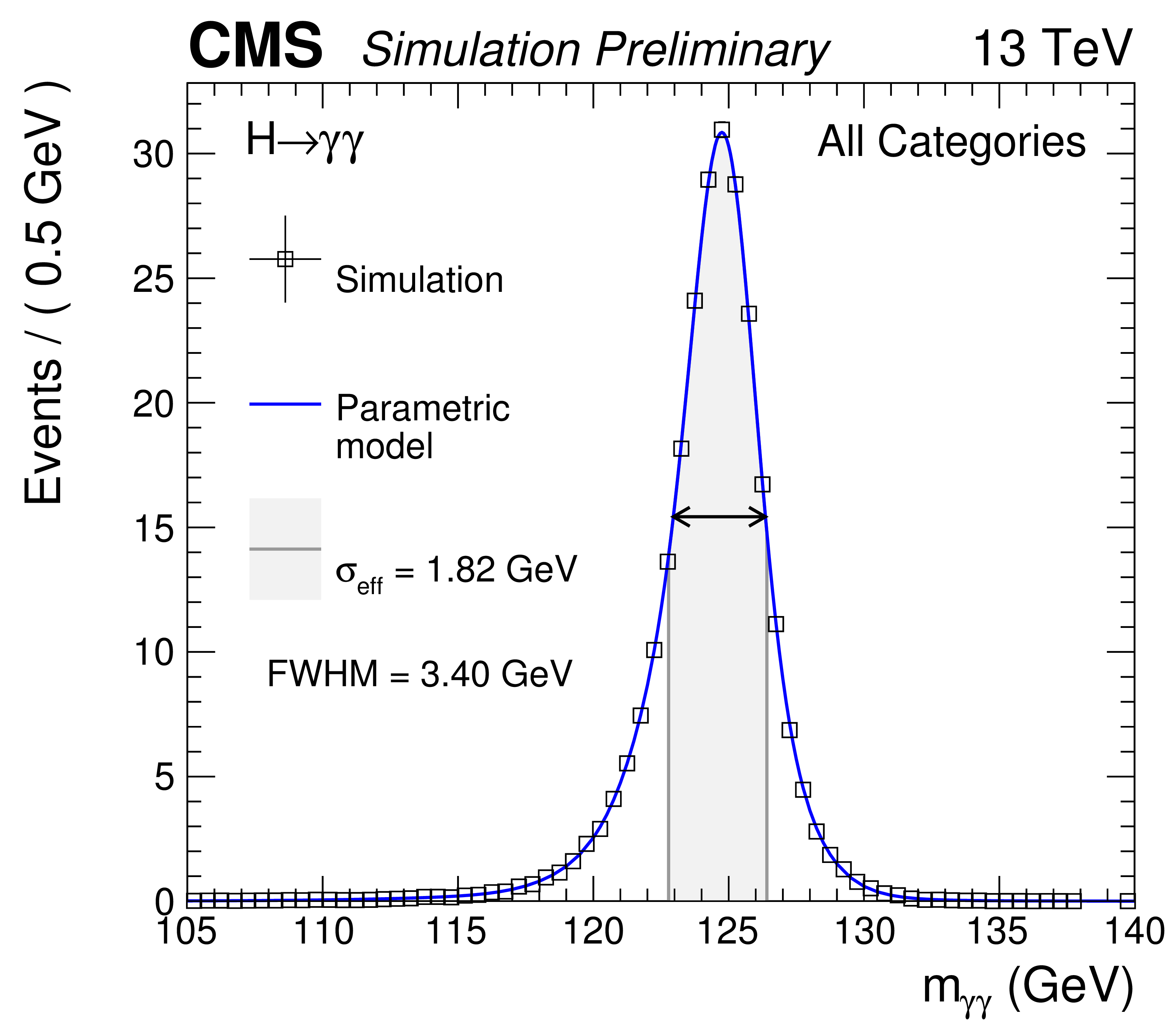
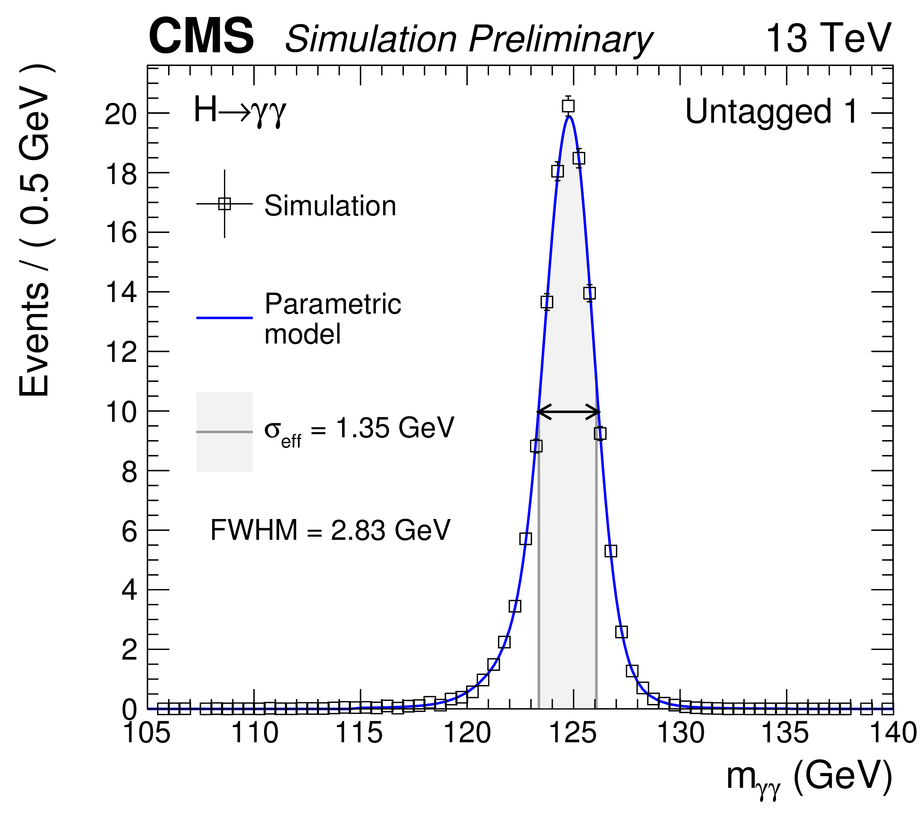
Figure 6-a:
Parametrized signal shape for the best resolution category (a) and for all categories combined together (b) for a simulated H$\to \gamma \gamma $ signal sample with $ {m_{\mathrm {H}} }= $ 125 GeV. The black points represent weighted simulation events and the blue lines are the corresponding models. Also shown are the $\sigma _{eff}$ value (half the width of the narrowest interval containing 68.3% of the invariant mass distribution), FWHM and the corresponding interval. |

png pdf |
Figure 6-b:
Parametrized signal shape for the best resolution category (a) and for all categories combined together (b) for a simulated H$\to \gamma \gamma $ signal sample with $ {m_{\mathrm {H}} }= $ 125 GeV. The black points represent weighted simulation events and the blue lines are the corresponding models. Also shown are the $\sigma _{eff}$ value (half the width of the narrowest interval containing 68.3% of the invariant mass distribution), FWHM and the corresponding interval. |

png pdf |
Figure 7:
The efficiency$\times $acceptance of the signal model as a function of $ {m_{\mathrm {H}} }$ for all categories combined. |

png pdf |
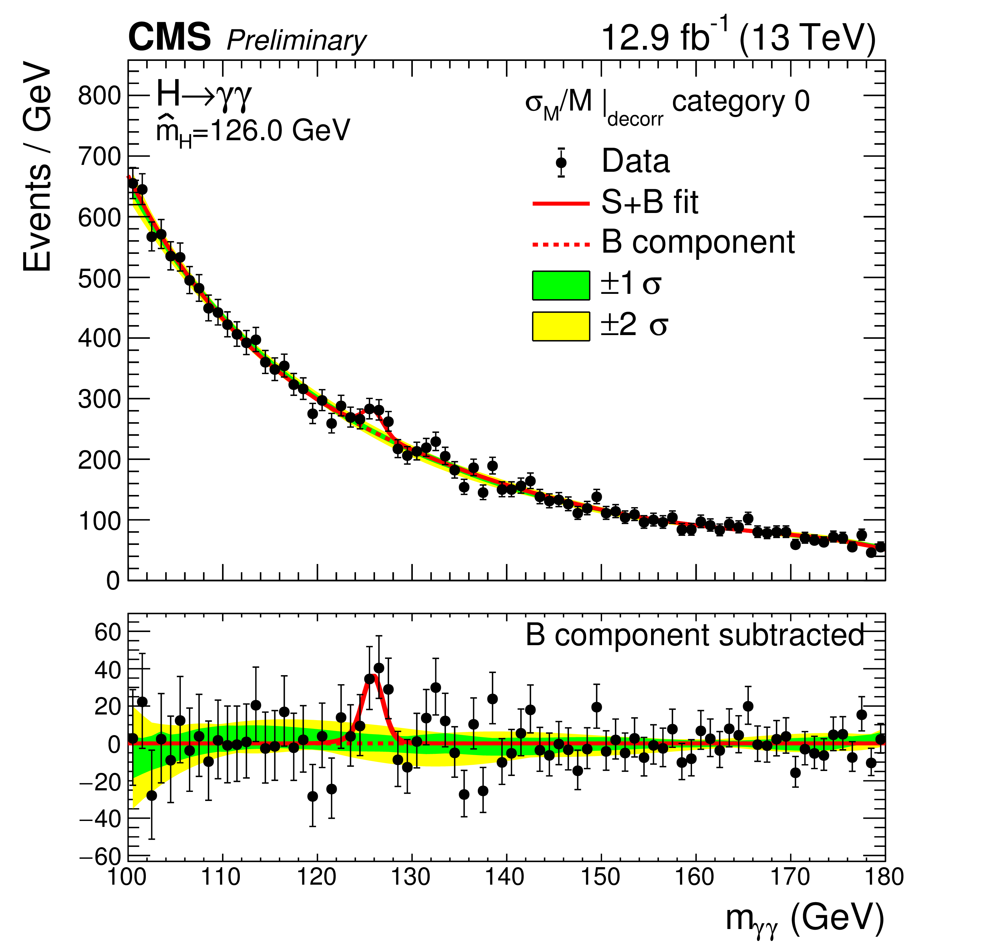
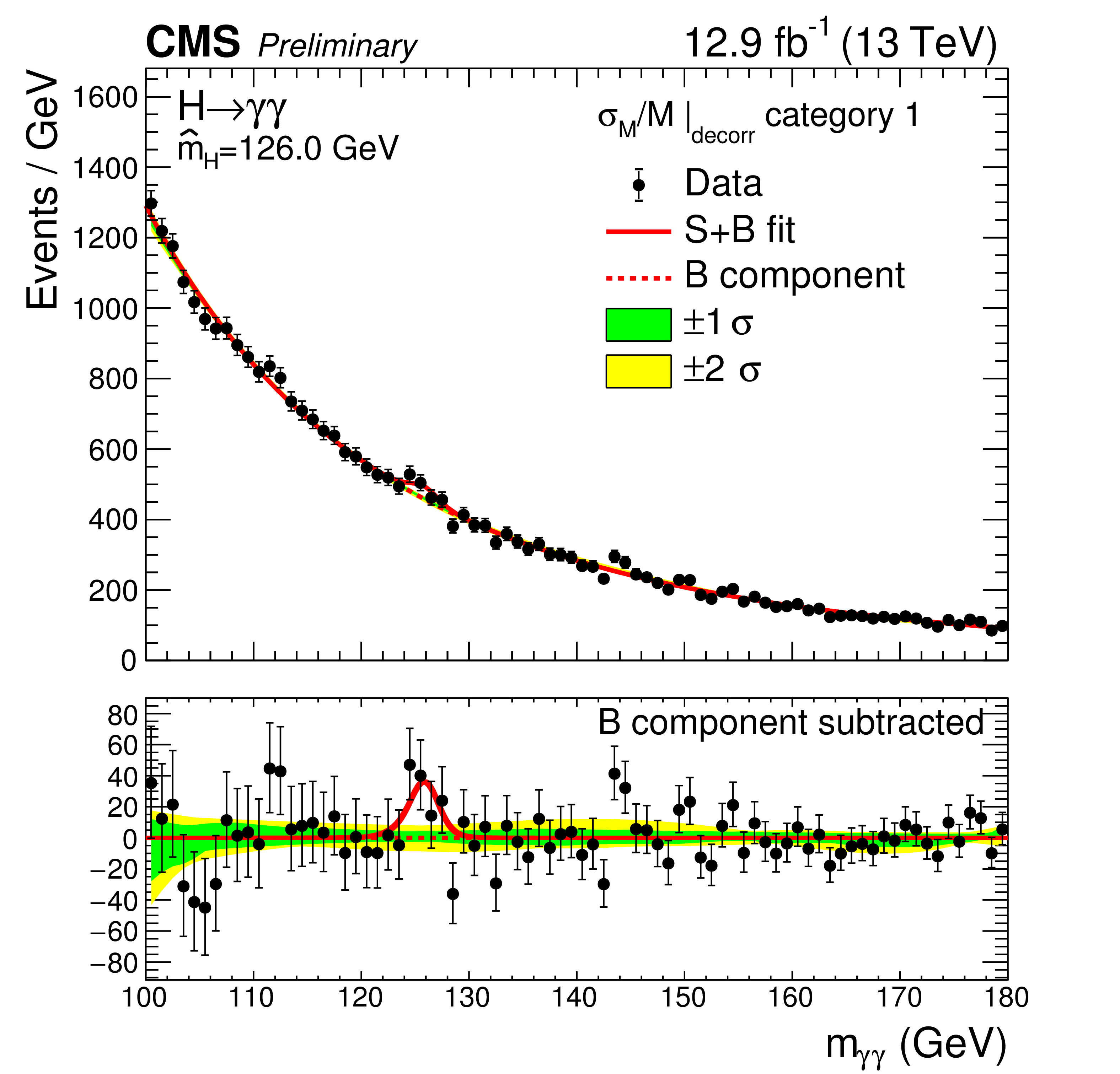
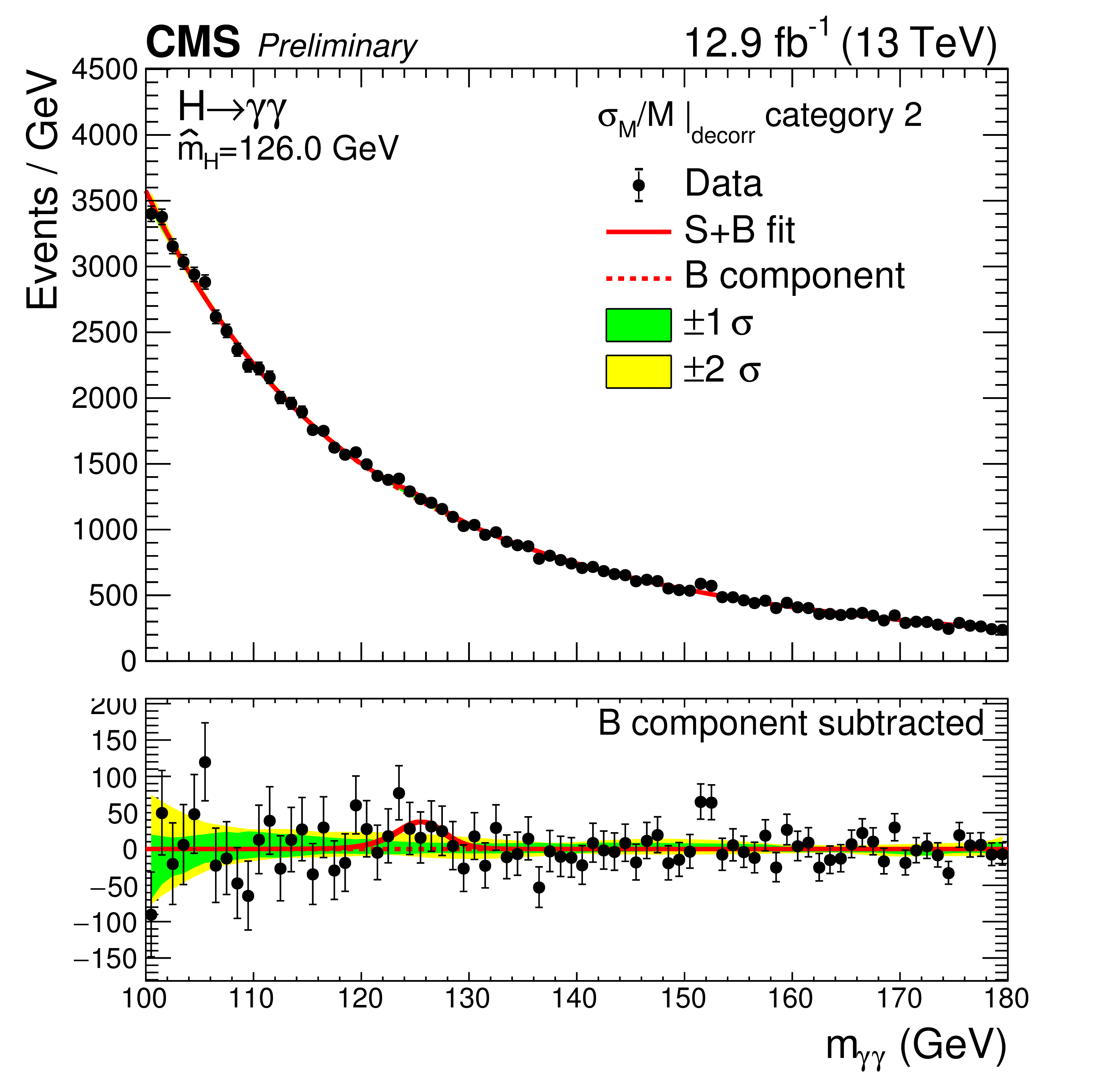
Figure 8-a:
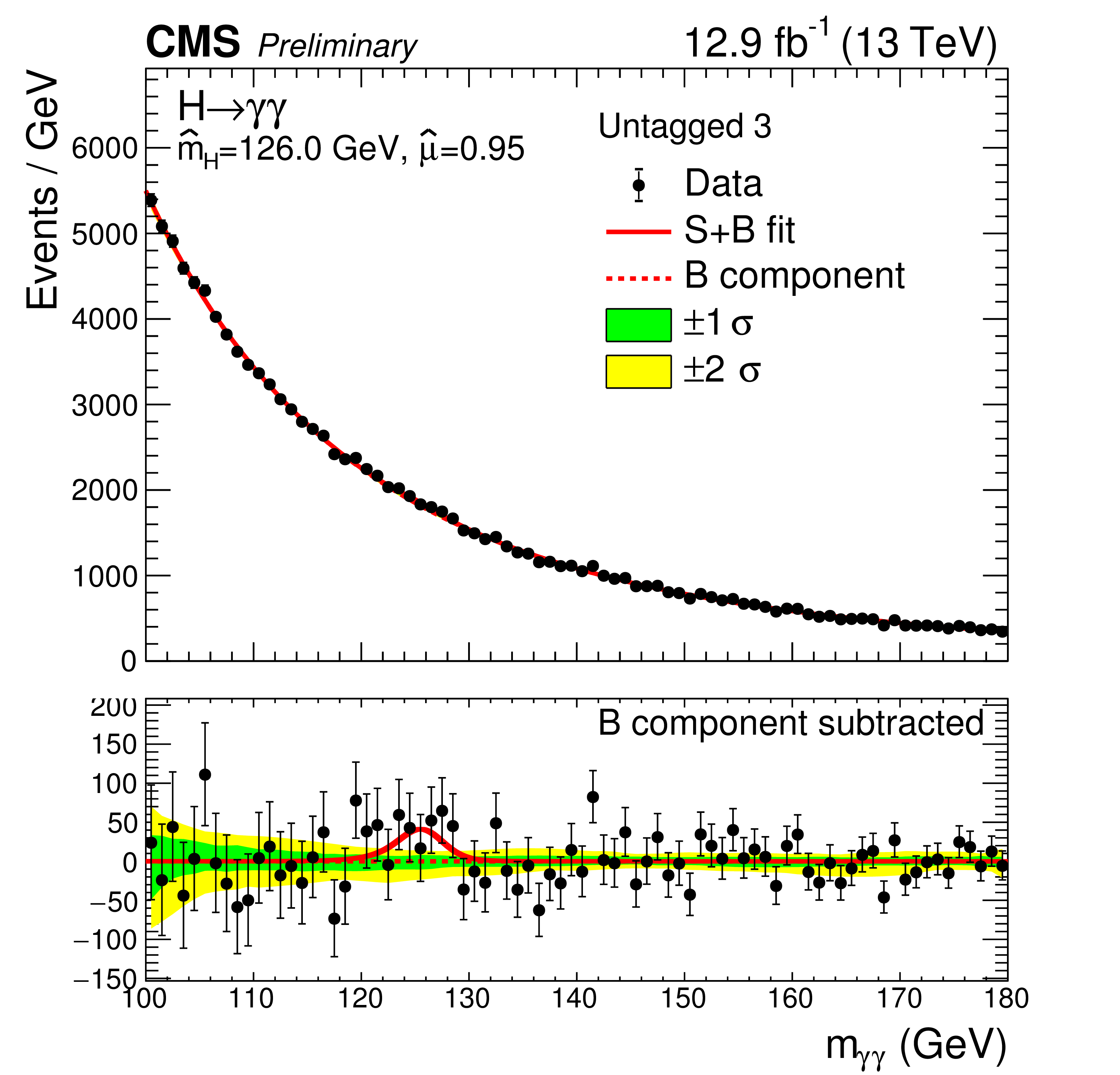
Data points (black) and signal plus background model fits in the four untagged categories are shown. The 1 standard deviation (green) and 2 standard deviation bands (yellow) include the uncertainties of the fit. The bottom plot shows the residuals after background subtraction. |

png pdf |
Figure 8-b:
Data points (black) and signal plus background model fits in the four untagged categories are shown. The 1 standard deviation (green) and 2 standard deviation bands (yellow) include the uncertainties of the fit. The bottom plot shows the residuals after background subtraction. |

png pdf |
Figure 8-c:
Data points (black) and signal plus background model fits in the four untagged categories are shown. The 1 standard deviation (green) and 2 standard deviation bands (yellow) include the uncertainties of the fit. The bottom plot shows the residuals after background subtraction. |
png pdf |
Figure 8-d:
Data points (black) and signal plus background model fits in the four untagged categories are shown. The 1 standard deviation (green) and 2 standard deviation bands (yellow) include the uncertainties of the fit. The bottom plot shows the residuals after background subtraction. |
png pdf |
Figure 9-a:
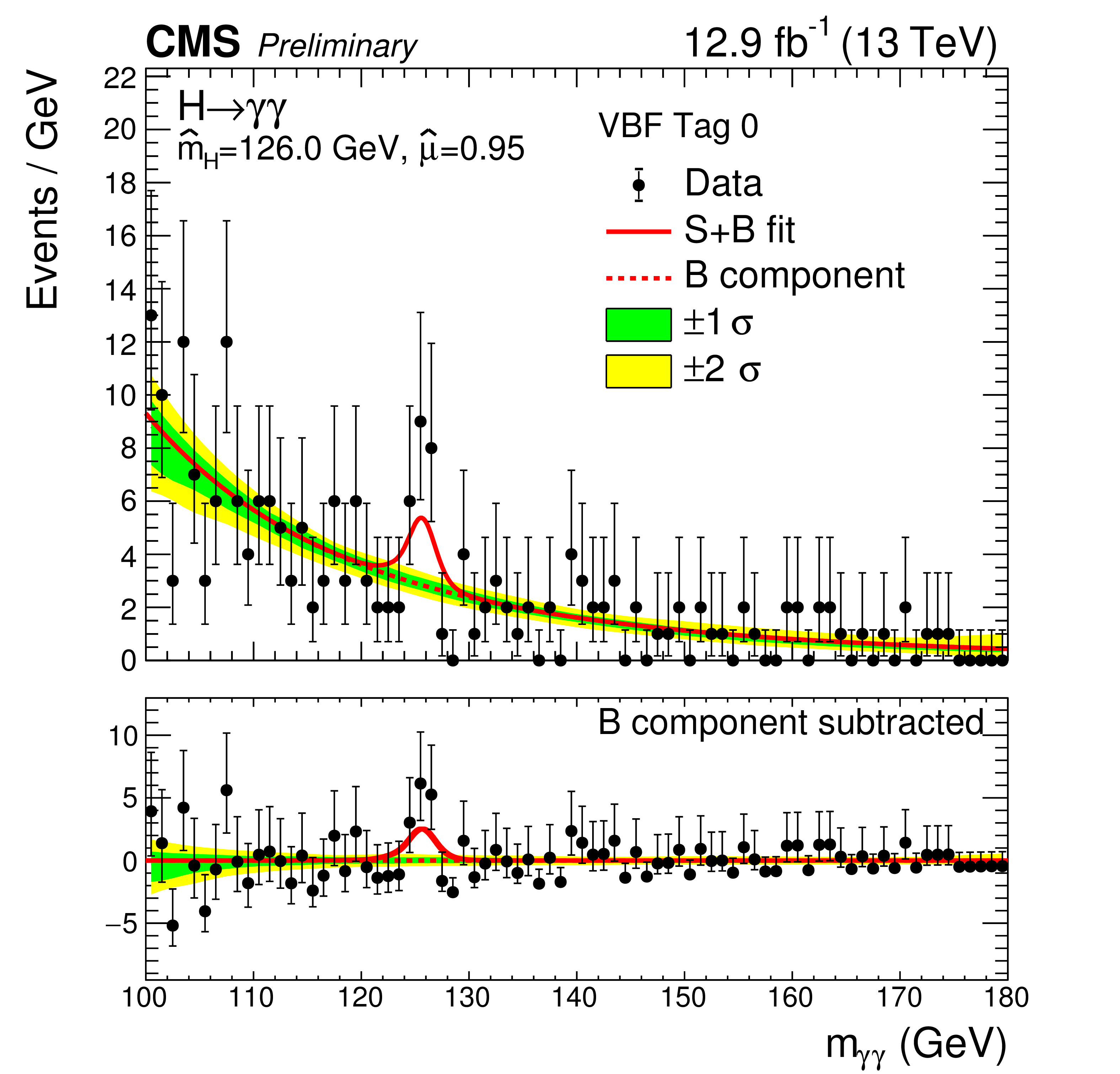
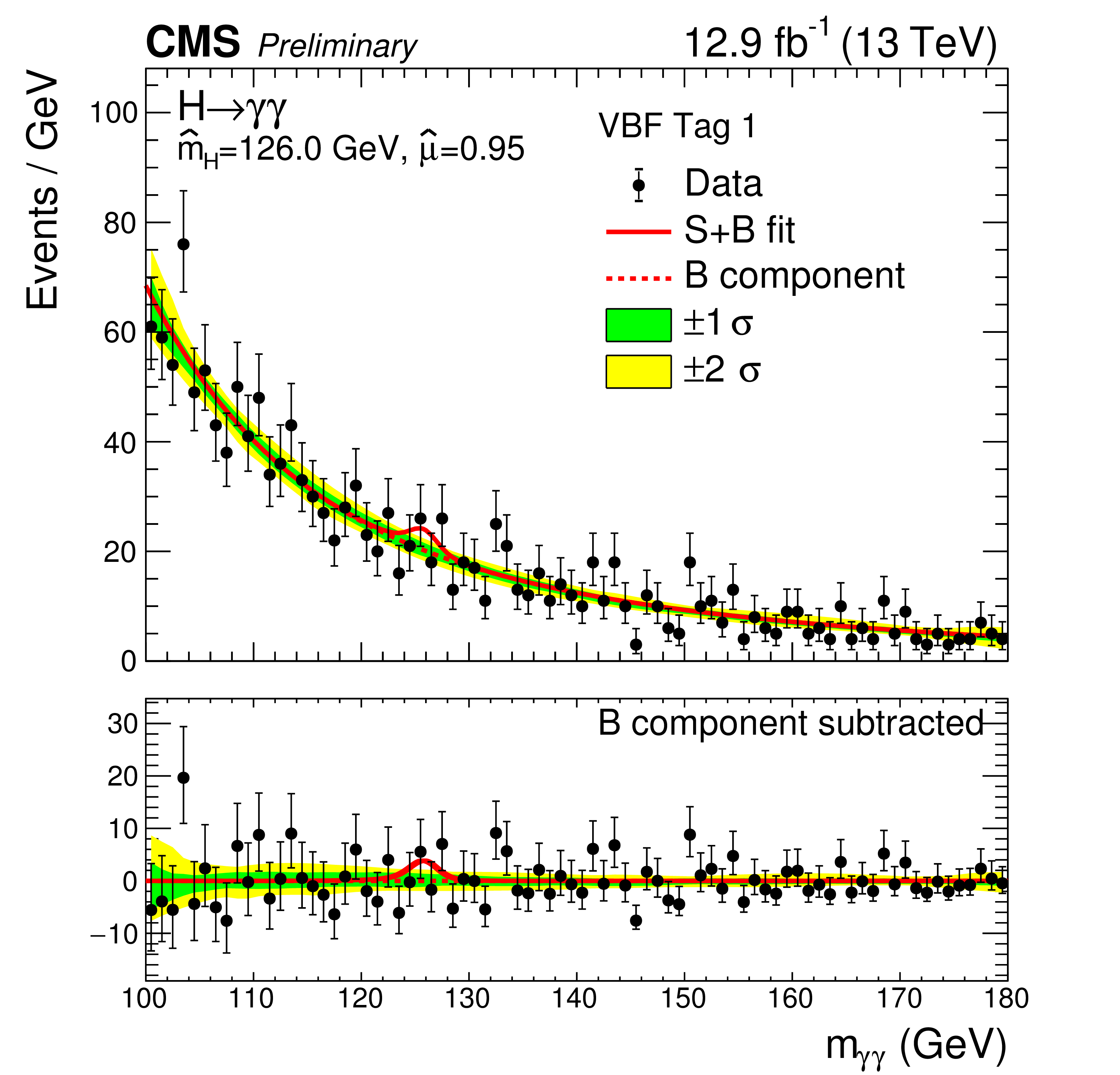
Data points (black) and signal plus background model fits in VBF and $\mathrm {t\bar{t}H}$ categories are shown. The 1 standard deviation (green) and 2 standard deviation bands (yellow) include the uncertainties of the fit. The bottom plot shows the residuals after background subtraction. |
png pdf |
Figure 9-b:
Data points (black) and signal plus background model fits in VBF and $\mathrm {t\bar{t}H}$ categories are shown. The 1 standard deviation (green) and 2 standard deviation bands (yellow) include the uncertainties of the fit. The bottom plot shows the residuals after background subtraction. |

png pdf |
Figure 9-c:
Data points (black) and signal plus background model fits in VBF and $\mathrm {t\bar{t}H}$ categories are shown. The 1 standard deviation (green) and 2 standard deviation bands (yellow) include the uncertainties of the fit. The bottom plot shows the residuals after background subtraction. |

png pdf |
Figure 9-d:
Data points (black) and signal plus background model fits in VBF and $\mathrm {t\bar{t}H}$ categories are shown. The 1 standard deviation (green) and 2 standard deviation bands (yellow) include the uncertainties of the fit. The bottom plot shows the residuals after background subtraction. |

png pdf |
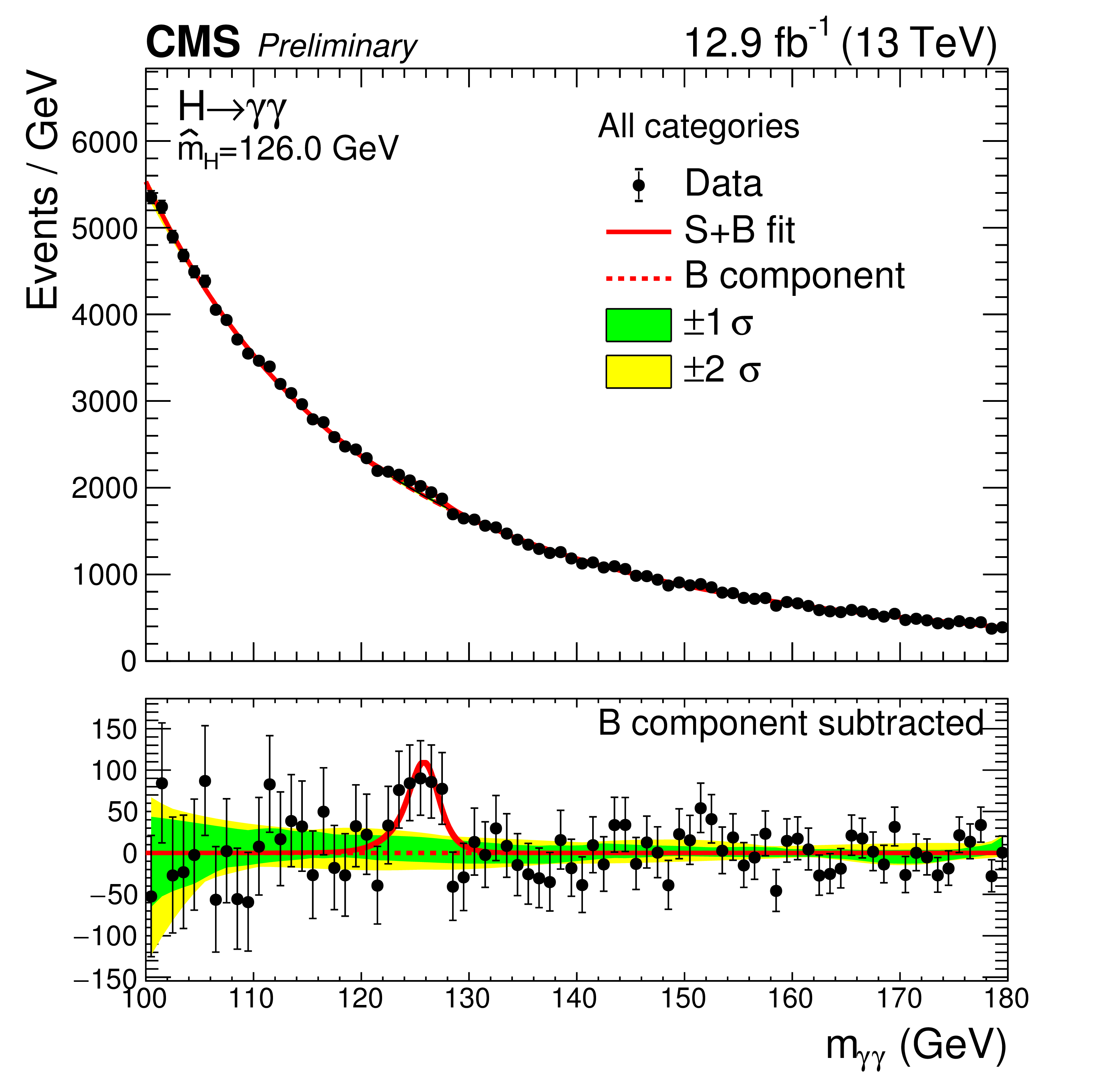
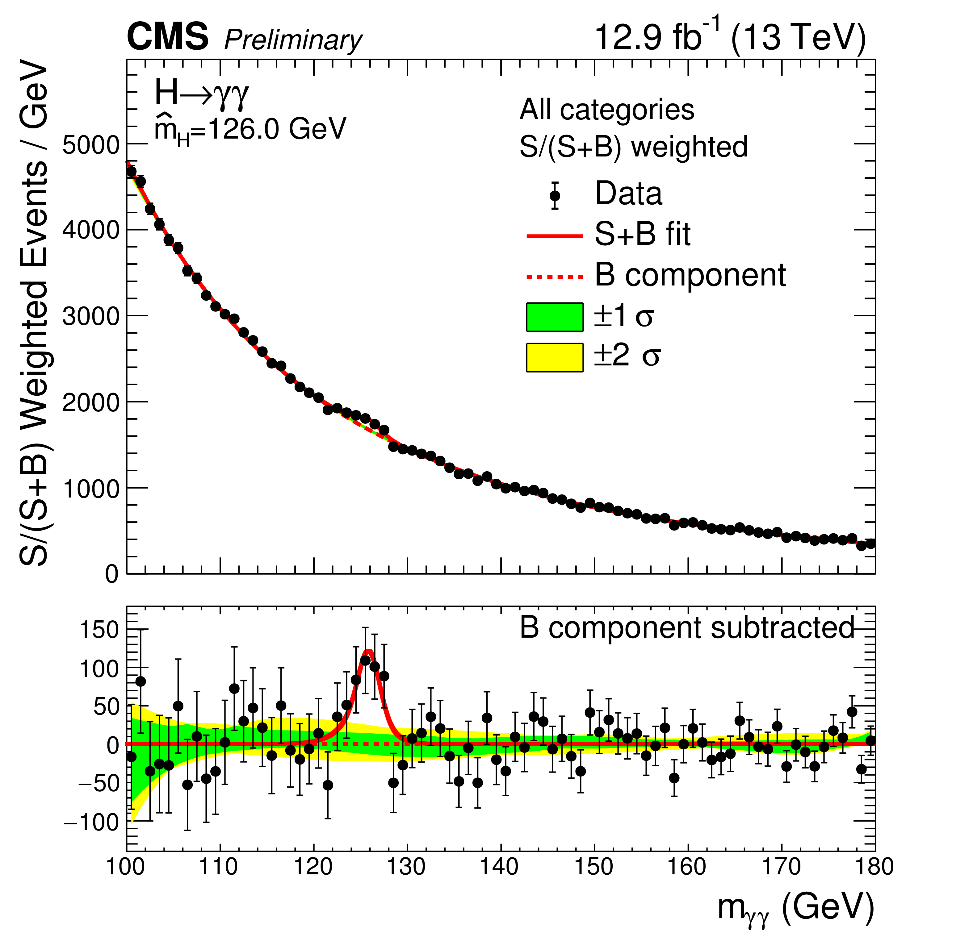
Figure 10-a:
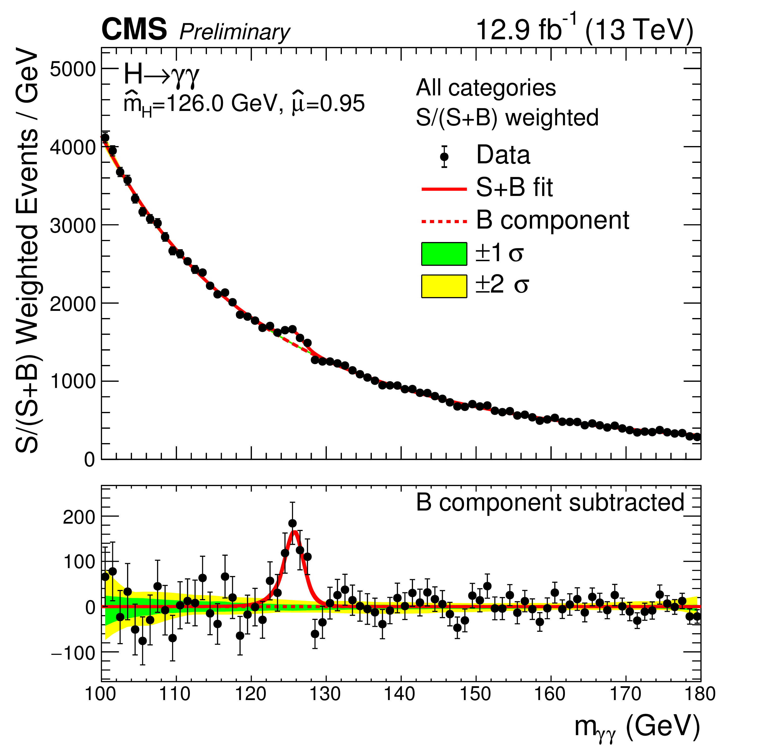
Data points (black) and signal plus background model fits for all categories summed (left) and where the categories are summed weighted by their sensitivity (right). The 1 standard deviation (green) and 2 standard deviation bands (yellow) include the uncertainties of the fit. The bottom plot shows the residuals after background subtraction. |
png pdf |
Figure 10-b:
Data points (black) and signal plus background model fits for all categories summed (left) and where the categories are summed weighted by their sensitivity (right). The 1 standard deviation (green) and 2 standard deviation bands (yellow) include the uncertainties of the fit. The bottom plot shows the residuals after background subtraction. |
png pdf |
Figure 11:
The observed p-value (black) is compared to the SM expectation across the fit range 120-130GeV, where the SM Higgs boson is assumed to have a mass $m_{\mathrm{H}}=125.09$GeV (blue). The red line shows the maximum significance for each mass hypothesis in the range $120$GeV$ |
png pdf |
Figure 12:
The likelihood scan for the signal strength where the value of the standard model Higgs boson mass is profiled in the fit. |

png pdf |
Figure 13:
Signal strength modifiers measured in each category (black points) for profiled $m_{\mathrm{H}}$, compared to the overall signal strength (green band) and to the SM expectation (dashed red line). |
png pdf |
Figure 14:
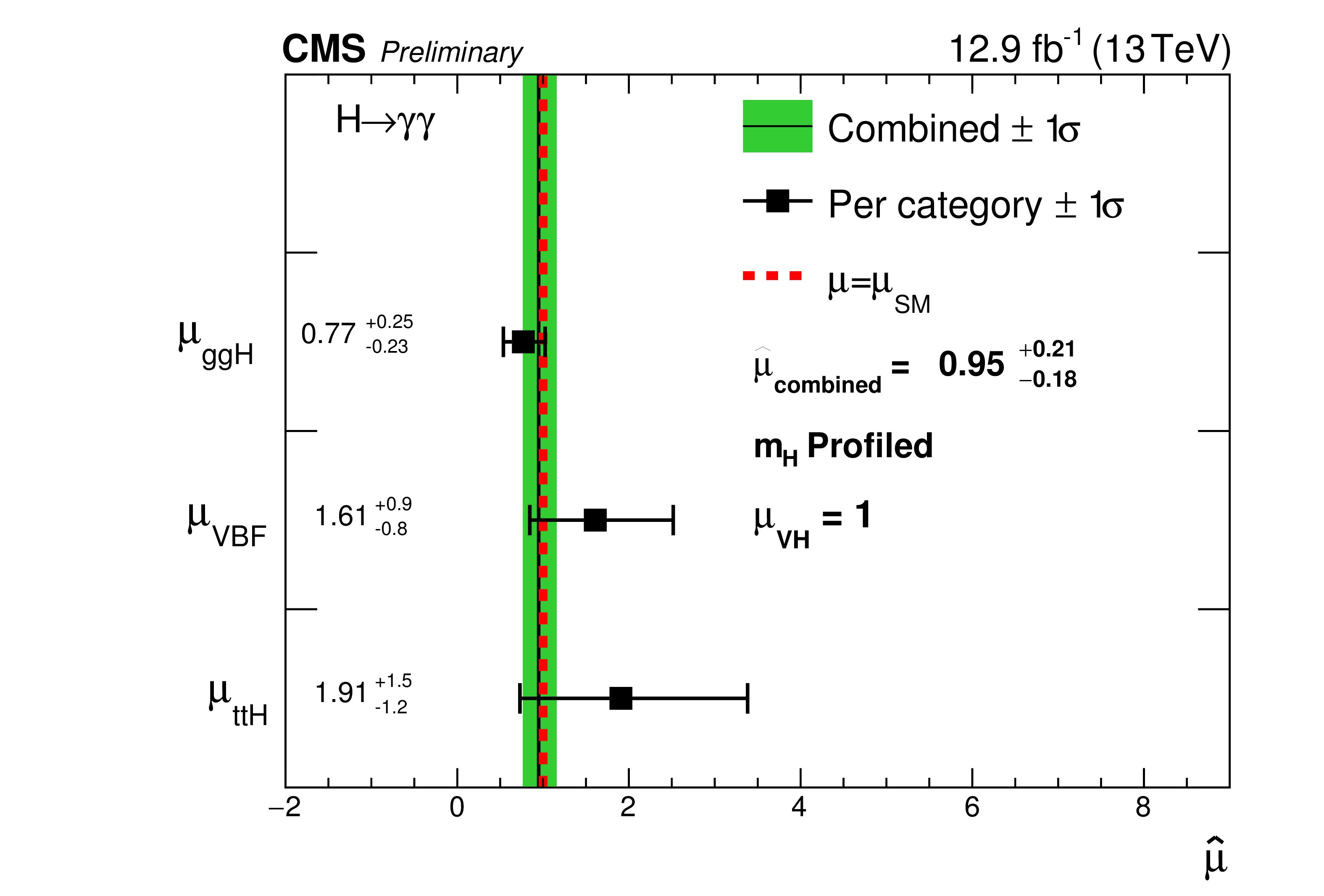
Signal strength modifiers measured for each process (black points) for profiled $m_{\mathrm{H}}$, compared to the overall signal strength (green band) and to the SM expectation (dashed red line). Since this analysis does include any categories targeting the VH process, we impose $\mu _{\text {VH}} =1$. |

png pdf |
Figure 15:
The two-dimensional best-fit (black cross) of the signal strengths for fermionic (ggH, $\mathrm {t\bar{t}H}$) and bosonic (VBF, ZH, WH) production modes compared to the SM expectations (red diamond). The Higgs boson mass is profiled in the fit. The solid (dashed) line represents the 1 standard deviation (2 standard deviation) confidence region. |

png pdf |
Figure 16-a:
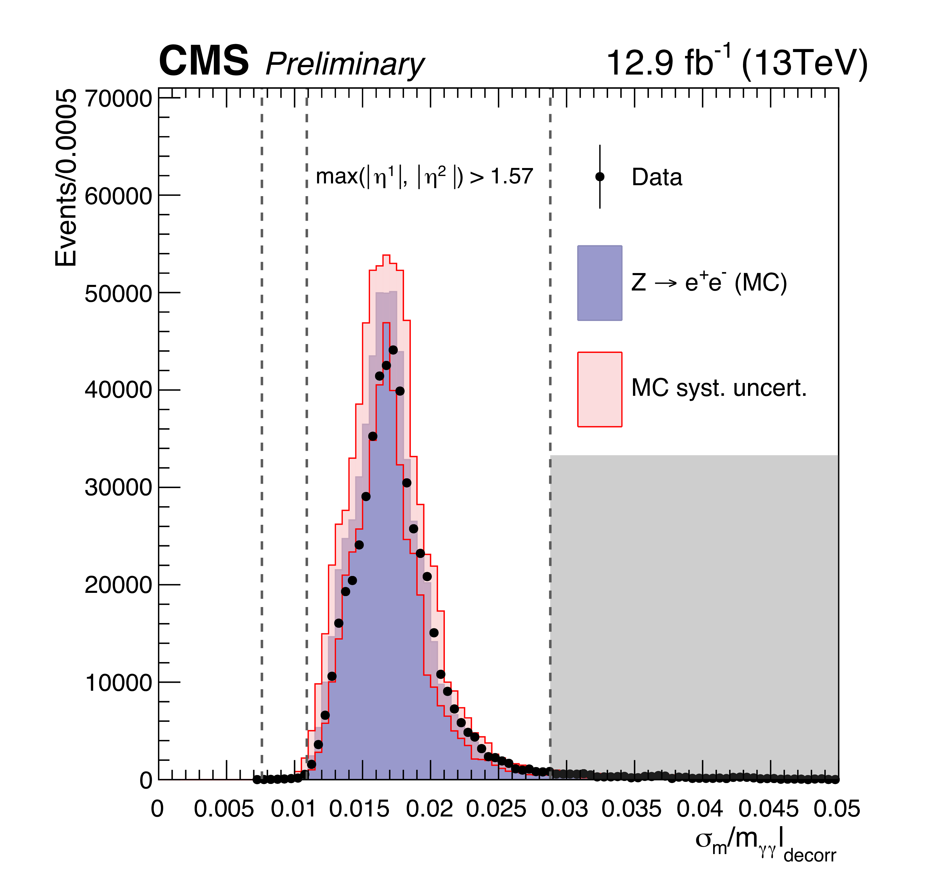
The distribution of the $ {\sigma _{M}/M }_{\textup {decorr}} $ for Z$\rightarrow $ e$^{+}$e$^{-}$ events, where electrons are reconstructed as photons, for events where both electrons are reconstructed in the ECAL barrel region (a) and for all remaining events (b). The red hashed region represents the systematic uncertainty resulting from the impact on the mass of the systematic uncertainty assigned to the per-photon energy resolution. Events in the gray region are discarded. |
png pdf |
Figure 16-b:
The distribution of the $ {\sigma _{M}/M }_{\textup {decorr}} $ for Z$\rightarrow $ e$^{+}$e$^{-}$ events, where electrons are reconstructed as photons, for events where both electrons are reconstructed in the ECAL barrel region (a) and for all remaining events (b). The red hashed region represents the systematic uncertainty resulting from the impact on the mass of the systematic uncertainty assigned to the per-photon energy resolution. Events in the gray region are discarded. |
png pdf |
Figure 17-a:
Fits of the distributions of the diphoton invariant mass for a simulated sample of Higgs bosons at $m_{\mathrm{H}}=$ 125 GeV for the category with the best resolution (left) and for all categories combined. |
png pdf |
Figure 17-b:
Fits of the distributions of the diphoton invariant mass for a simulated sample of Higgs bosons at $m_{\mathrm{H}}=$ 125 GeV for the category with the best resolution (left) and for all categories combined. |
png pdf |
Figure 18-a:
Data points (black) and signal plus background model fits in each of the categories used for the fiducial analysis are shown. The 1 standard deviation (green) and 2 standard deviation bands (yellow) include the uncertainties of the fit. The bottom plot shows the residuals after background subtraction. |
png pdf |
Figure 18-b:
Data points (black) and signal plus background model fits in each of the categories used for the fiducial analysis are shown. The 1 standard deviation (green) and 2 standard deviation bands (yellow) include the uncertainties of the fit. The bottom plot shows the residuals after background subtraction. |
png pdf |
Figure 18-c:
Data points (black) and signal plus background model fits in each of the categories used for the fiducial analysis are shown. The 1 standard deviation (green) and 2 standard deviation bands (yellow) include the uncertainties of the fit. The bottom plot shows the residuals after background subtraction. |
png pdf |
Figure 19-a:
Data points (black) and signal plus background model fits for all the fiducial analysis categories summed (a) and where the categories are summed weighted by their sensitivity (b). The 1 standard deviation (green) and 2 standard deviation bands (yellow) include the uncertainties of the fit. The bottom plot shows the residuals after background subtraction. |
png pdf |
Figure 19-b:
Data points (black) and signal plus background model fits for all the fiducial analysis categories summed (a) and where the categories are summed weighted by their sensitivity (b). The 1 standard deviation (green) and 2 standard deviation bands (yellow) include the uncertainties of the fit. The bottom plot shows the residuals after background subtraction. |
png pdf |
Figure 20:
A likelihood scan for the fiducial cross section where the value of the standard model Higgs boson mass is profiled in the fit. The red line and hashed area represent the SM expected fiducial cross section and uncertainty for a Higgs boson of mass $m_{\mathrm{H}}=$ 125.09 GeV. The normalisation has been set using the latest values from [18] and the acceptance is defined using the aMC@NLO generator-level quantities. |

png pdf |
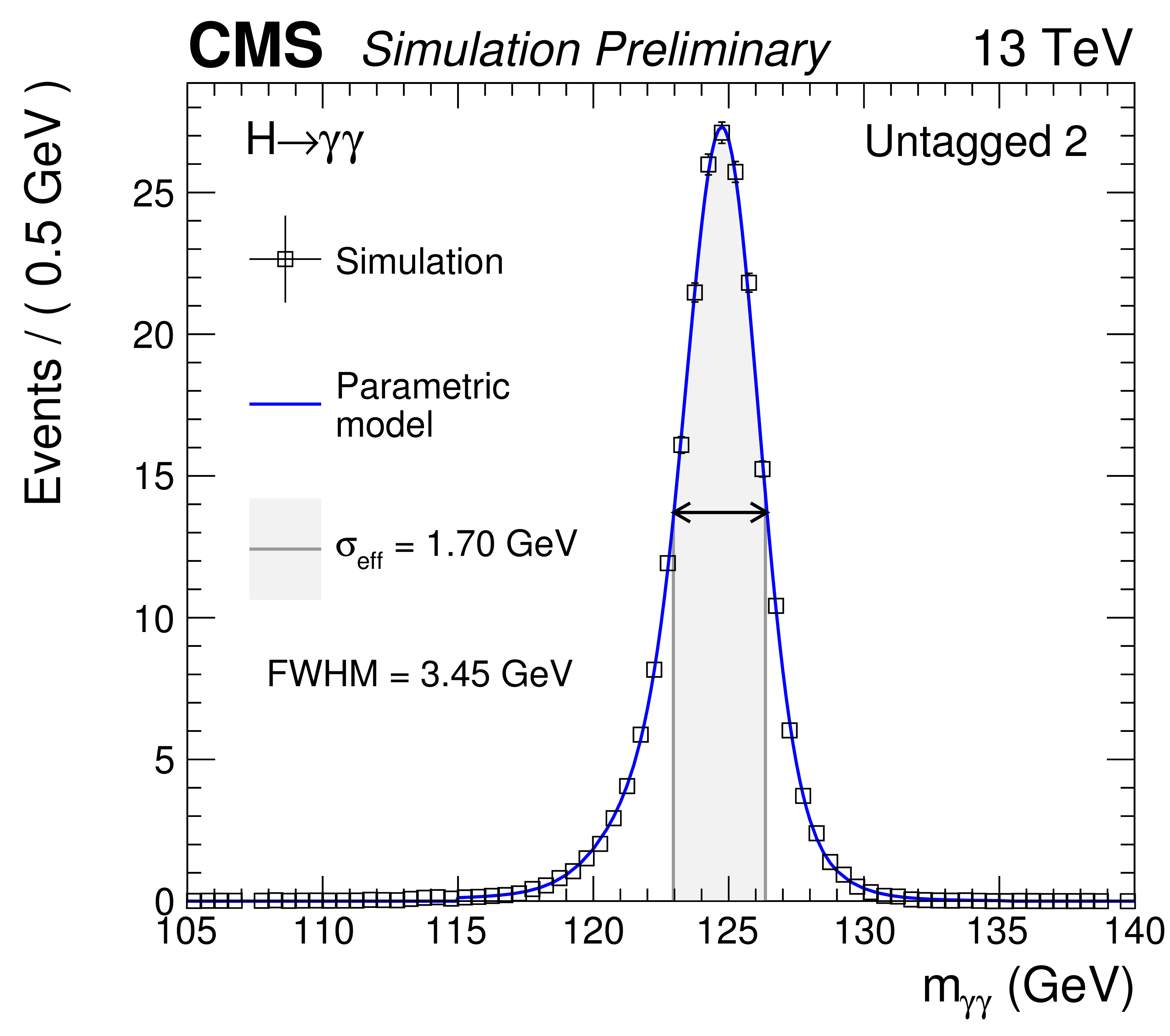
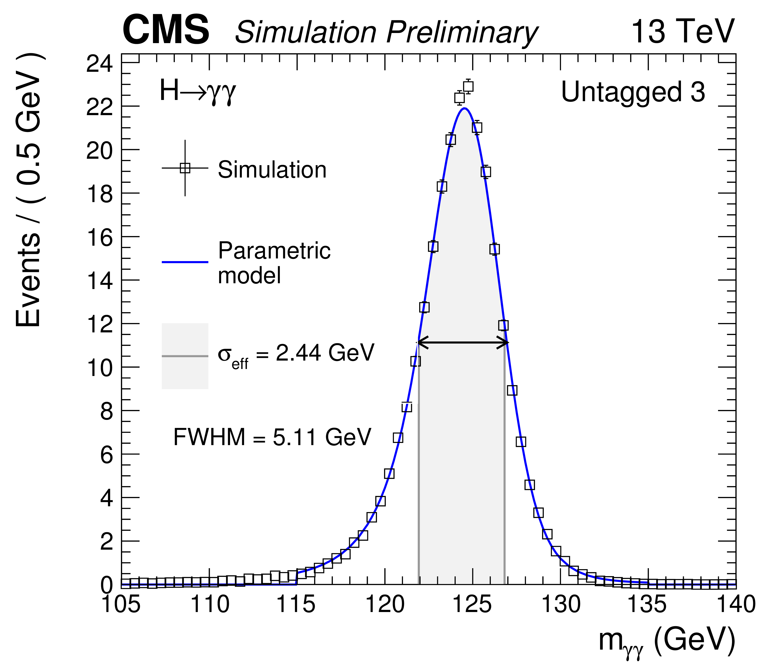
Figure 21-a:
Parametrized signal shapes for the inclusive categories, for a simulated H$\to \gamma \gamma $ signal sample with $ {m_{\mathrm {H}} }=$ 125 GeV. The black points represent weighted simulation events and the blue lines are the corresponding models. Also shown are the $\sigma _{eff}$ value (half the width of the narrowest interval containing 68.3% of the invariant mass distribution), FWHM and the corresponding interval. |
png pdf |
Figure 21-b:
Parametrized signal shapes for the inclusive categories, for a simulated H$\to \gamma \gamma $ signal sample with $ {m_{\mathrm {H}} }=$ 125 GeV. The black points represent weighted simulation events and the blue lines are the corresponding models. Also shown are the $\sigma _{eff}$ value (half the width of the narrowest interval containing 68.3% of the invariant mass distribution), FWHM and the corresponding interval. |
png pdf |
Figure 21-c:
Parametrized signal shapes for the inclusive categories, for a simulated H$\to \gamma \gamma $ signal sample with $ {m_{\mathrm {H}} }=$ 125 GeV. The black points represent weighted simulation events and the blue lines are the corresponding models. Also shown are the $\sigma _{eff}$ value (half the width of the narrowest interval containing 68.3% of the invariant mass distribution), FWHM and the corresponding interval. |
png pdf |
Figure 21-d:
Parametrized signal shapes for the inclusive categories, for a simulated H$\to \gamma \gamma $ signal sample with $ {m_{\mathrm {H}} }=$ 125 GeV. The black points represent weighted simulation events and the blue lines are the corresponding models. Also shown are the $\sigma _{eff}$ value (half the width of the narrowest interval containing 68.3% of the invariant mass distribution), FWHM and the corresponding interval. |
png pdf |
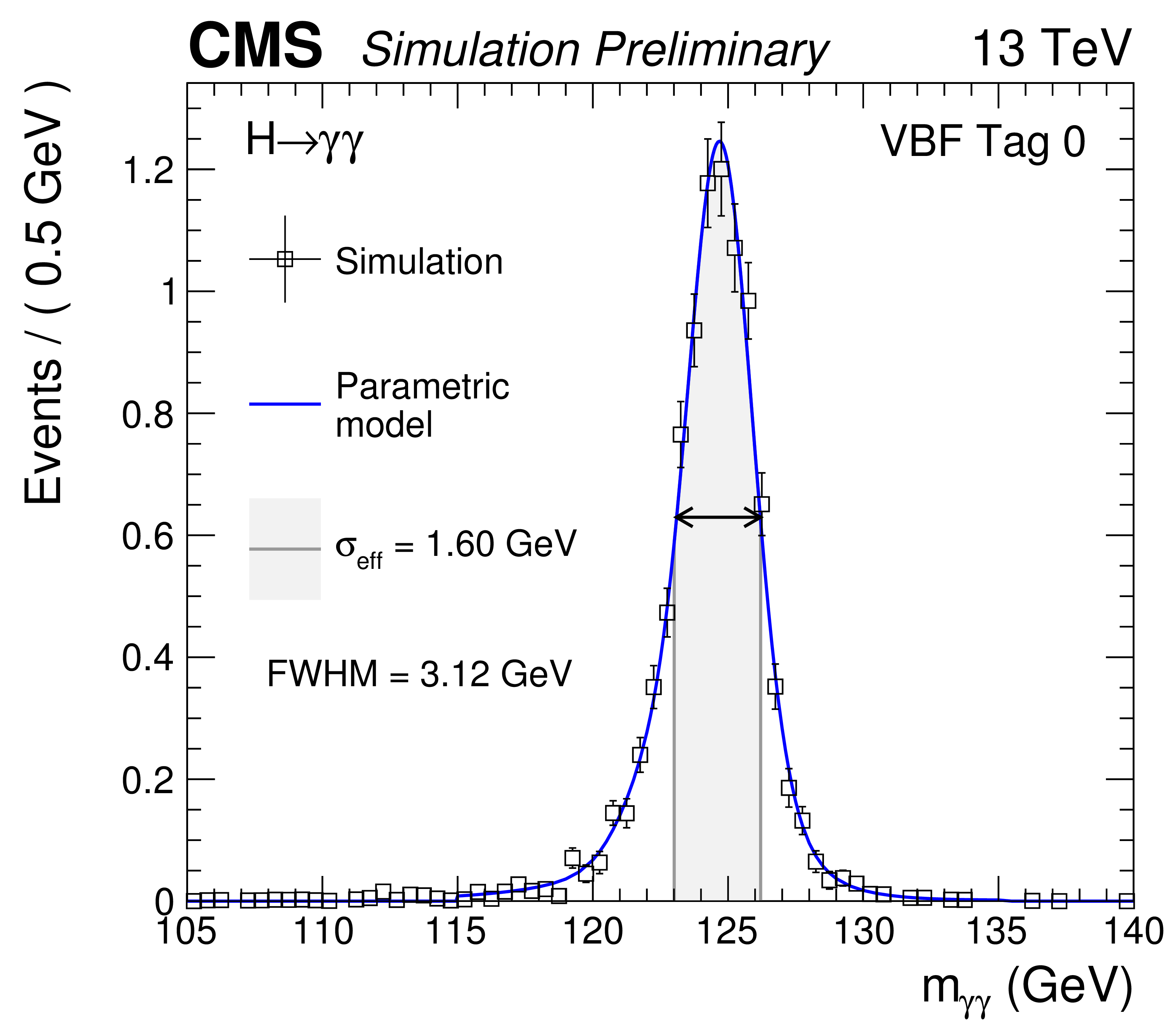
Figure 22-a:
Parametrized signal shapes for the VBF and TTH categories, for a simulated H$\to \gamma \gamma $ signal sample with $ {m_{\mathrm {H}} }=$ 125 GeV. The black points represent weighted simulation events and the blue lines are the corresponding models. Also shown are the $\sigma _{eff}$ value (half the width of the narrowest interval containing 68.3% of the invariant mass distribution), FWHM and the corresponding interval. |
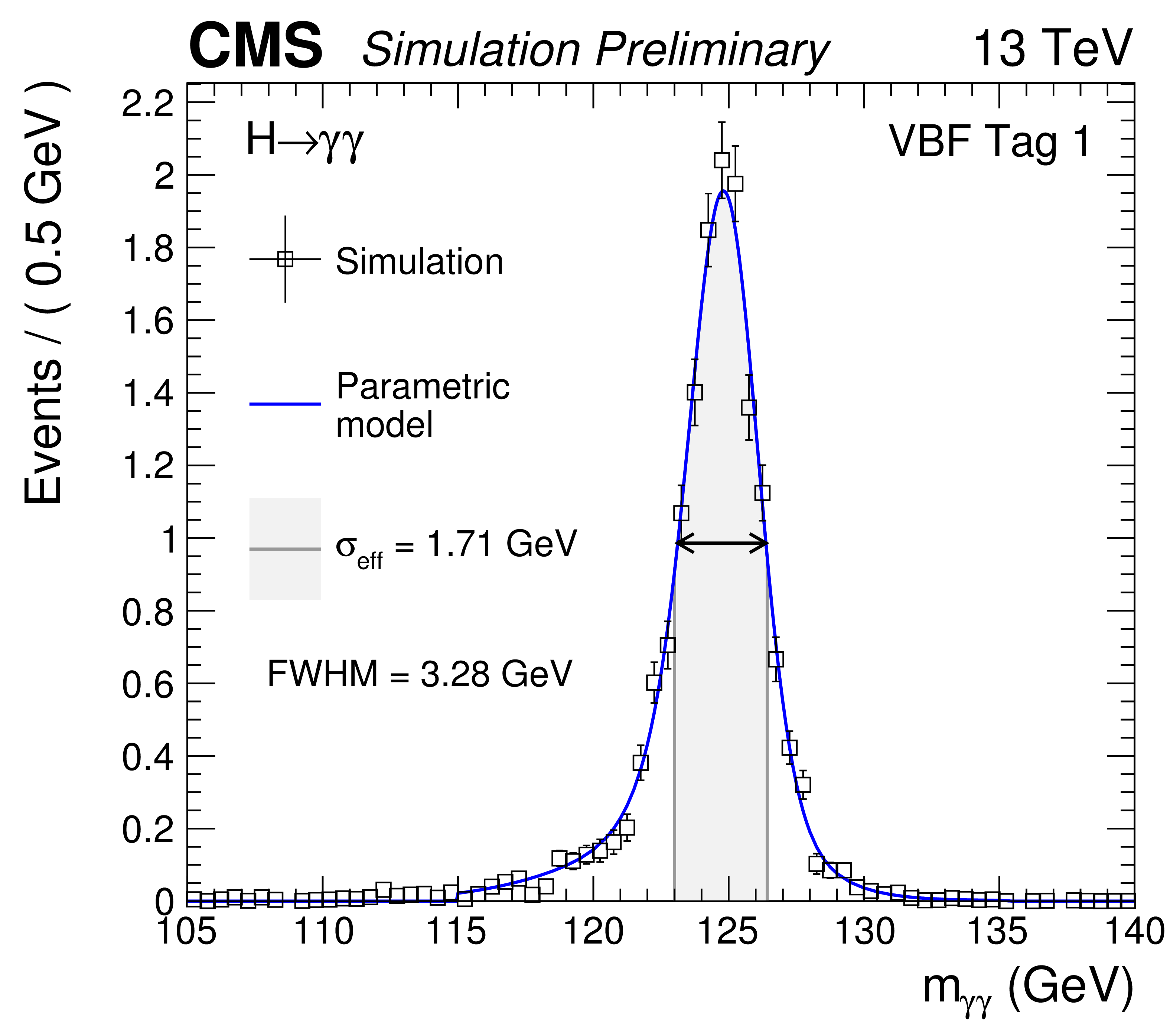
png pdf |
Figure 22-b:
Parametrized signal shapes for the VBF and TTH categories, for a simulated H$\to \gamma \gamma $ signal sample with $ {m_{\mathrm {H}} }=$ 125 GeV. The black points represent weighted simulation events and the blue lines are the corresponding models. Also shown are the $\sigma _{eff}$ value (half the width of the narrowest interval containing 68.3% of the invariant mass distribution), FWHM and the corresponding interval. |
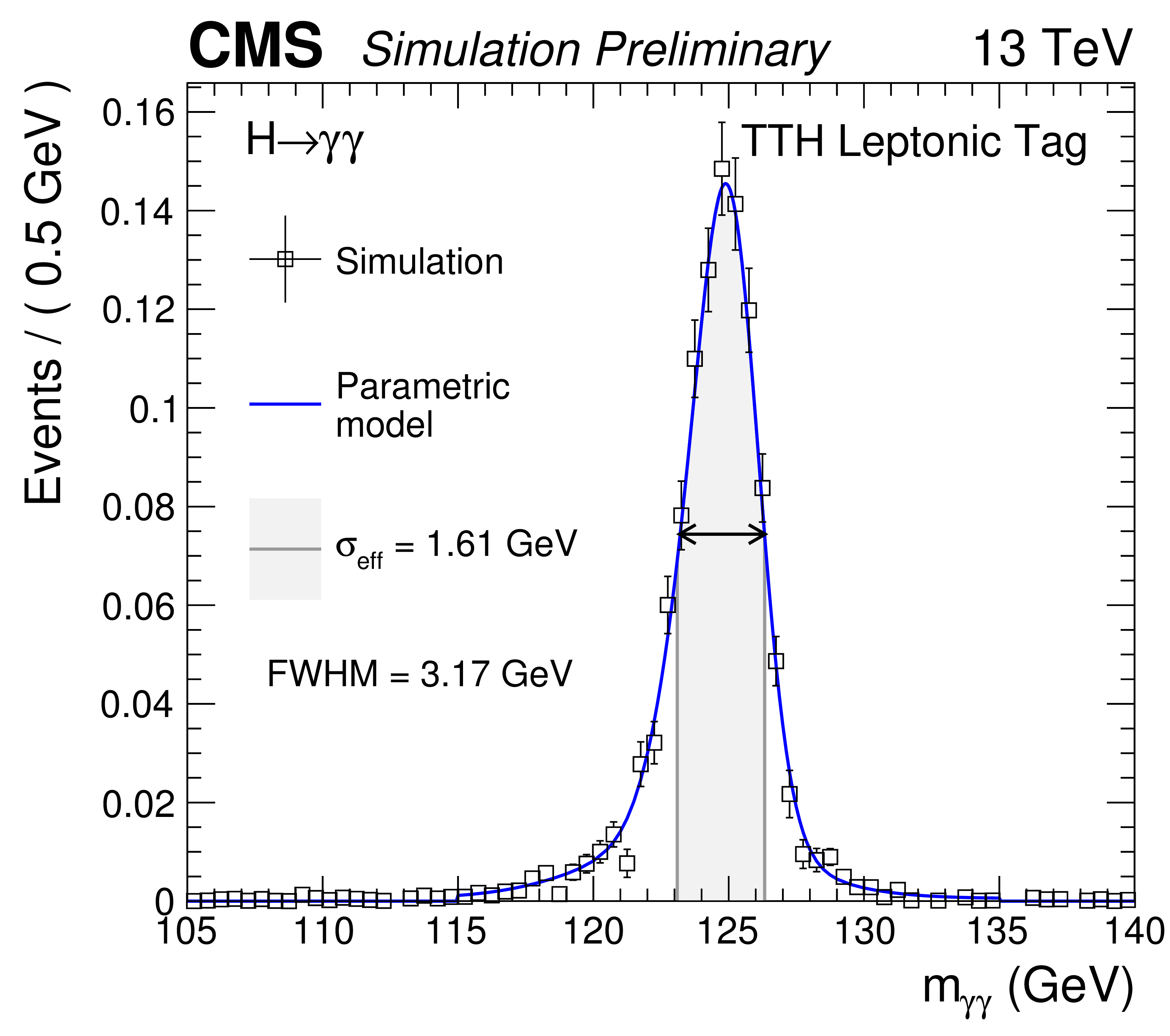
png pdf |
Figure 22-c:
Parametrized signal shapes for the VBF and TTH categories, for a simulated H$\to \gamma \gamma $ signal sample with $ {m_{\mathrm {H}} }=$ 125 GeV. The black points represent weighted simulation events and the blue lines are the corresponding models. Also shown are the $\sigma _{eff}$ value (half the width of the narrowest interval containing 68.3% of the invariant mass distribution), FWHM and the corresponding interval. |
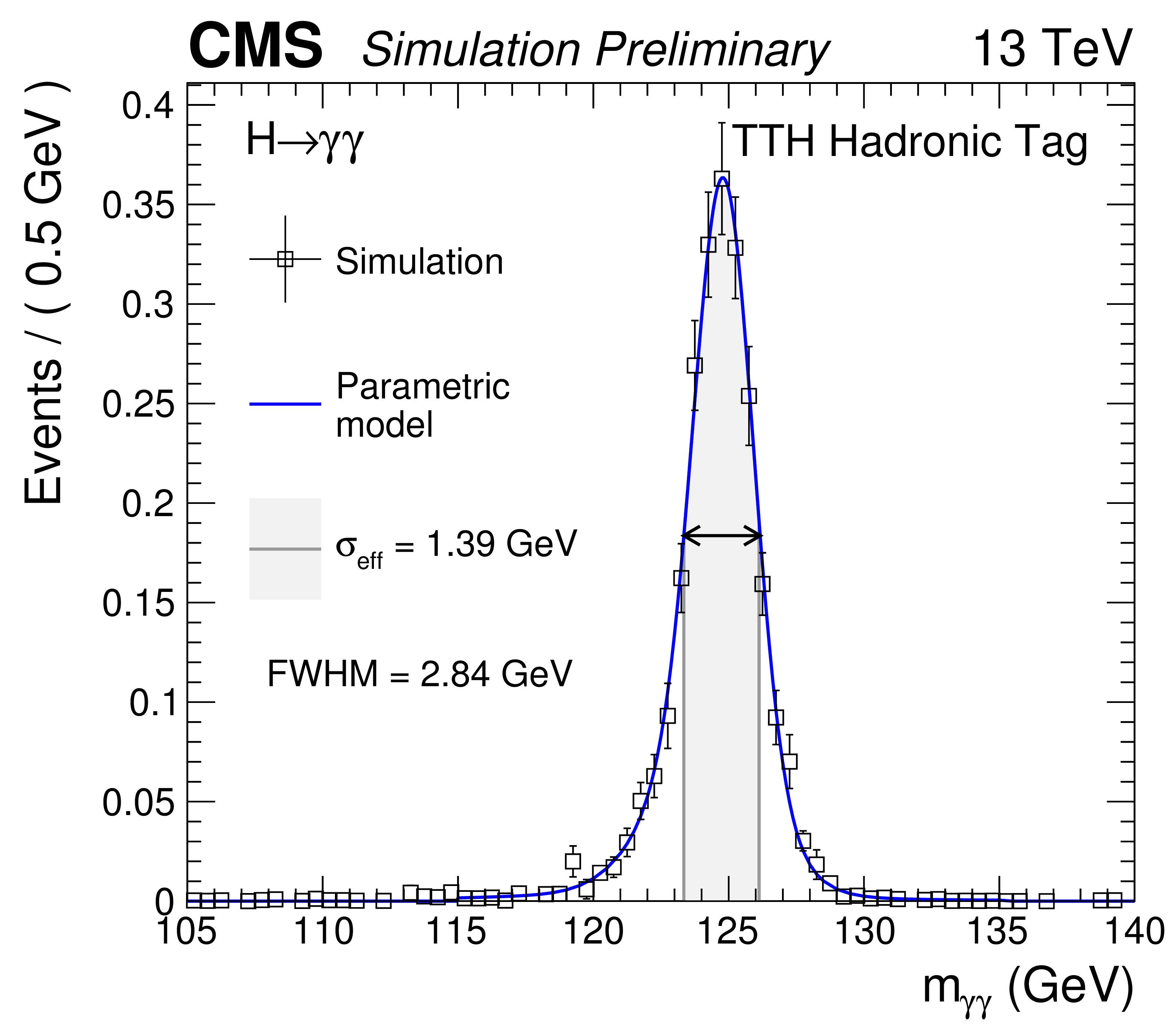
png pdf |
Figure 22-d:
Parametrized signal shapes for the VBF and TTH categories, for a simulated H$\to \gamma \gamma $ signal sample with $ {m_{\mathrm {H}} }=$ 125 GeV. The black points represent weighted simulation events and the blue lines are the corresponding models. Also shown are the $\sigma _{eff}$ value (half the width of the narrowest interval containing 68.3% of the invariant mass distribution), FWHM and the corresponding interval. |
png pdf |
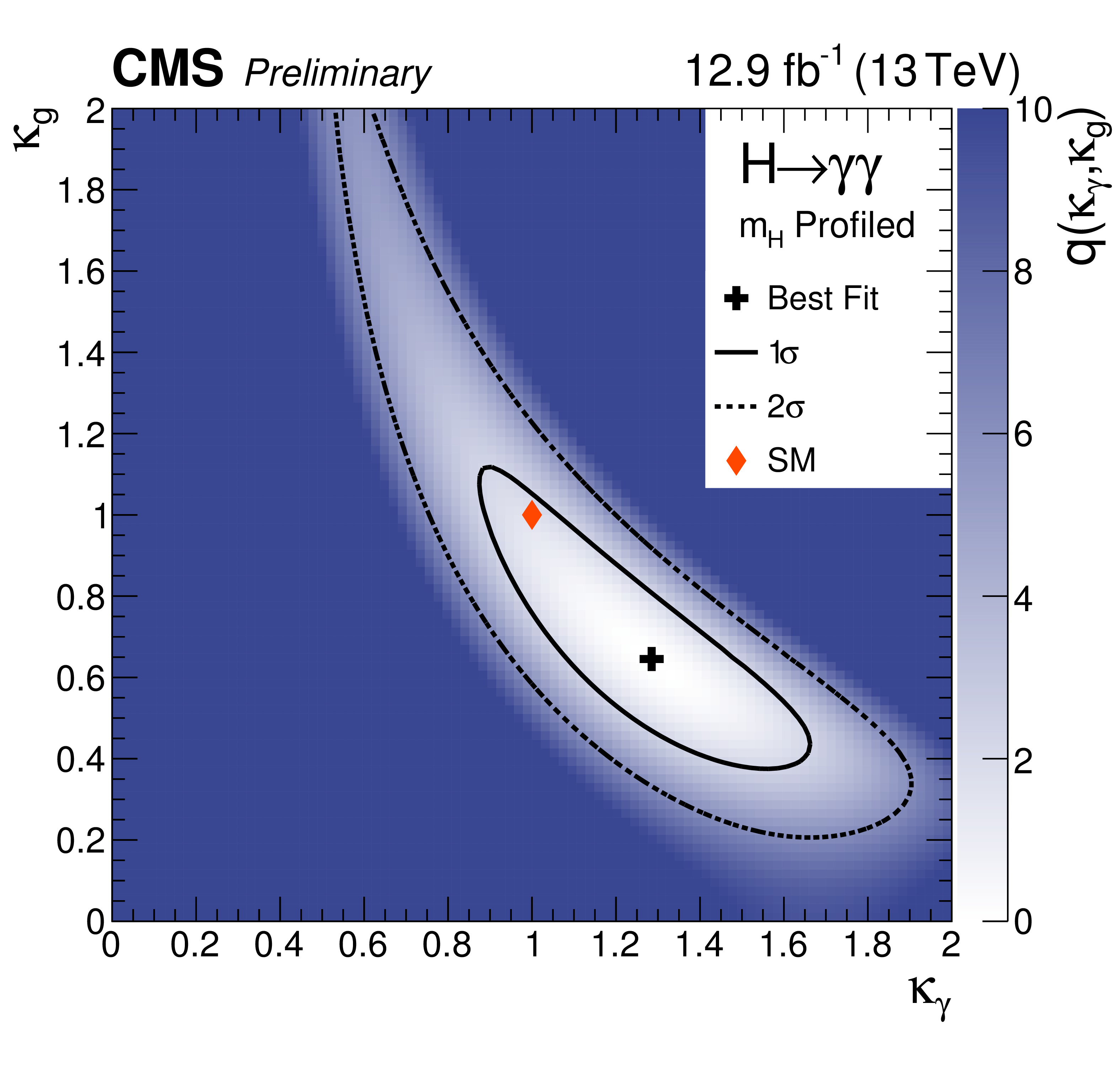
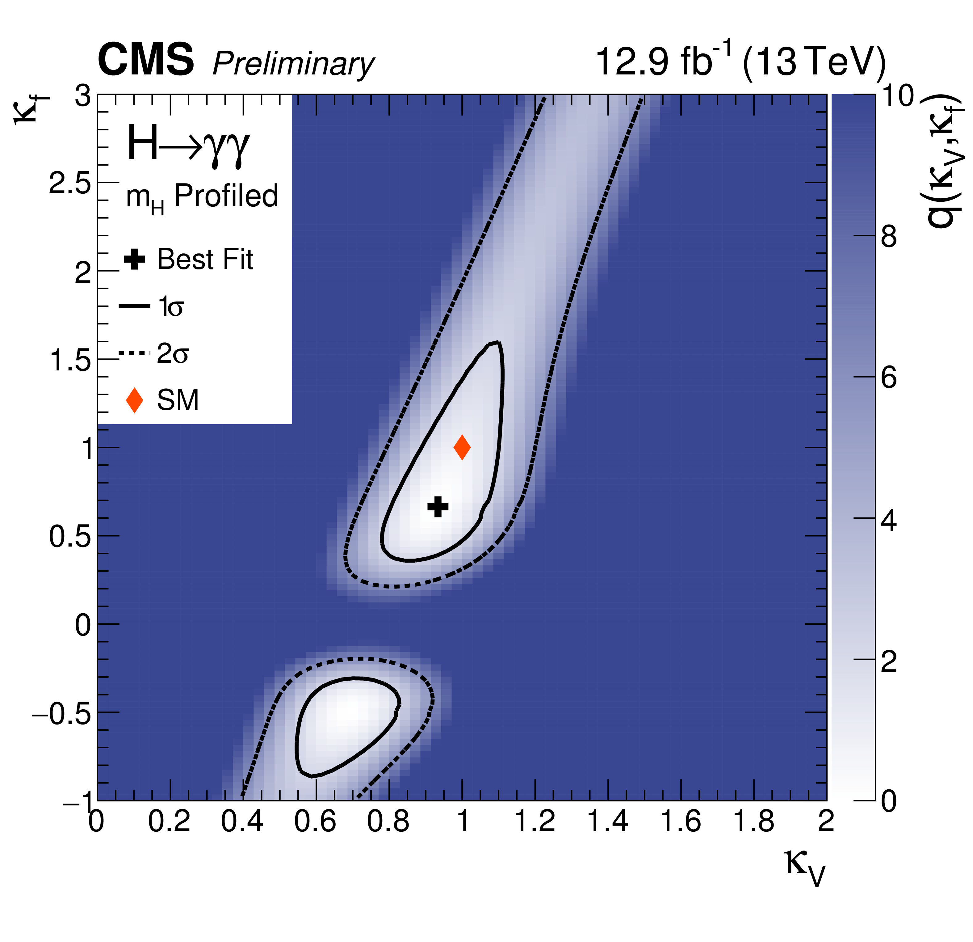
Figure 23-a:
Two-dimensional likelihood scans of $\kappa _{f}$ versus $\kappa _{V}$ (a) and $\kappa _{g}$ versus $\kappa _{\gamma }$ (b) are shown. The variables $\kappa _{V}$ and $\kappa _{f}$ are, respectively, the coupling modifiers of the Higgs boson to vector bosons and to fermions while $\kappa _{\gamma }$ and $\kappa _{g}$ are the effective coupling modifiers to photons and to gluons [36]. All four variables are expressed relative to the SM expectations. The mass of the Higgs boson is profiled in the fits. For each scan, the value of the Higgs boson mass is profiled The standard model expectation is marked with a red diamond. |
png pdf |
Figure 23-b:
Two-dimensional likelihood scans of $\kappa _{f}$ versus $\kappa _{V}$ (a) and $\kappa _{g}$ versus $\kappa _{\gamma }$ (b) are shown. The variables $\kappa _{V}$ and $\kappa _{f}$ are, respectively, the coupling modifiers of the Higgs boson to vector bosons and to fermions while $\kappa _{\gamma }$ and $\kappa _{g}$ are the effective coupling modifiers to photons and to gluons [36]. All four variables are expressed relative to the SM expectations. The mass of the Higgs boson is profiled in the fits. For each scan, the value of the Higgs boson mass is profiled The standard model expectation is marked with a red diamond. |
png pdf |
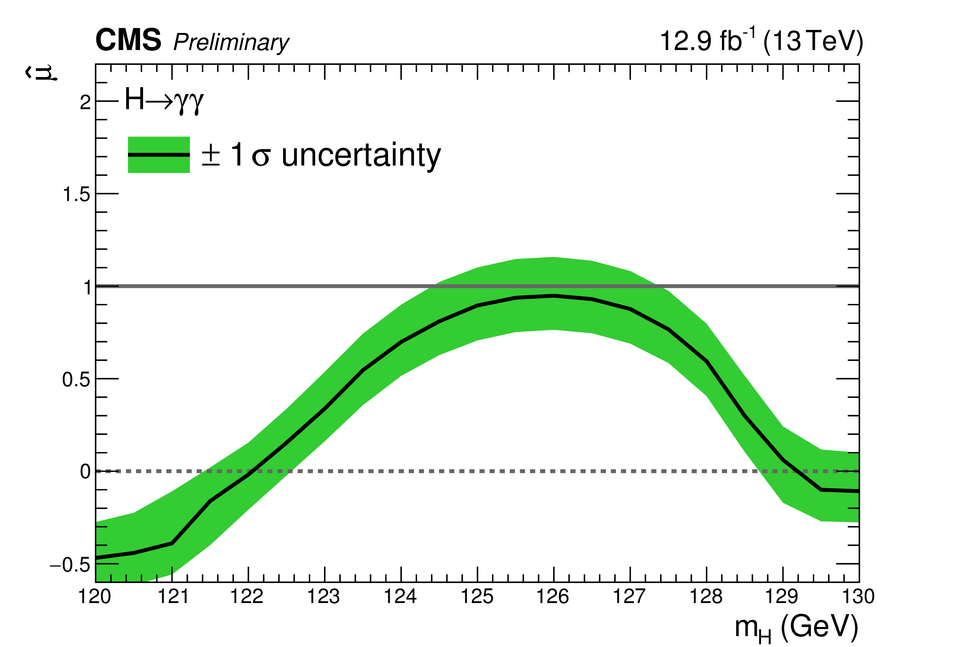
Figure 24:
The figure shows the result of performing a one-dimensional likelihood scan of the signal strength for various values of $m_{\mathrm{H}}$. The green band represents the uncertainties on the value of the signal strength at each point. |
png pdf |
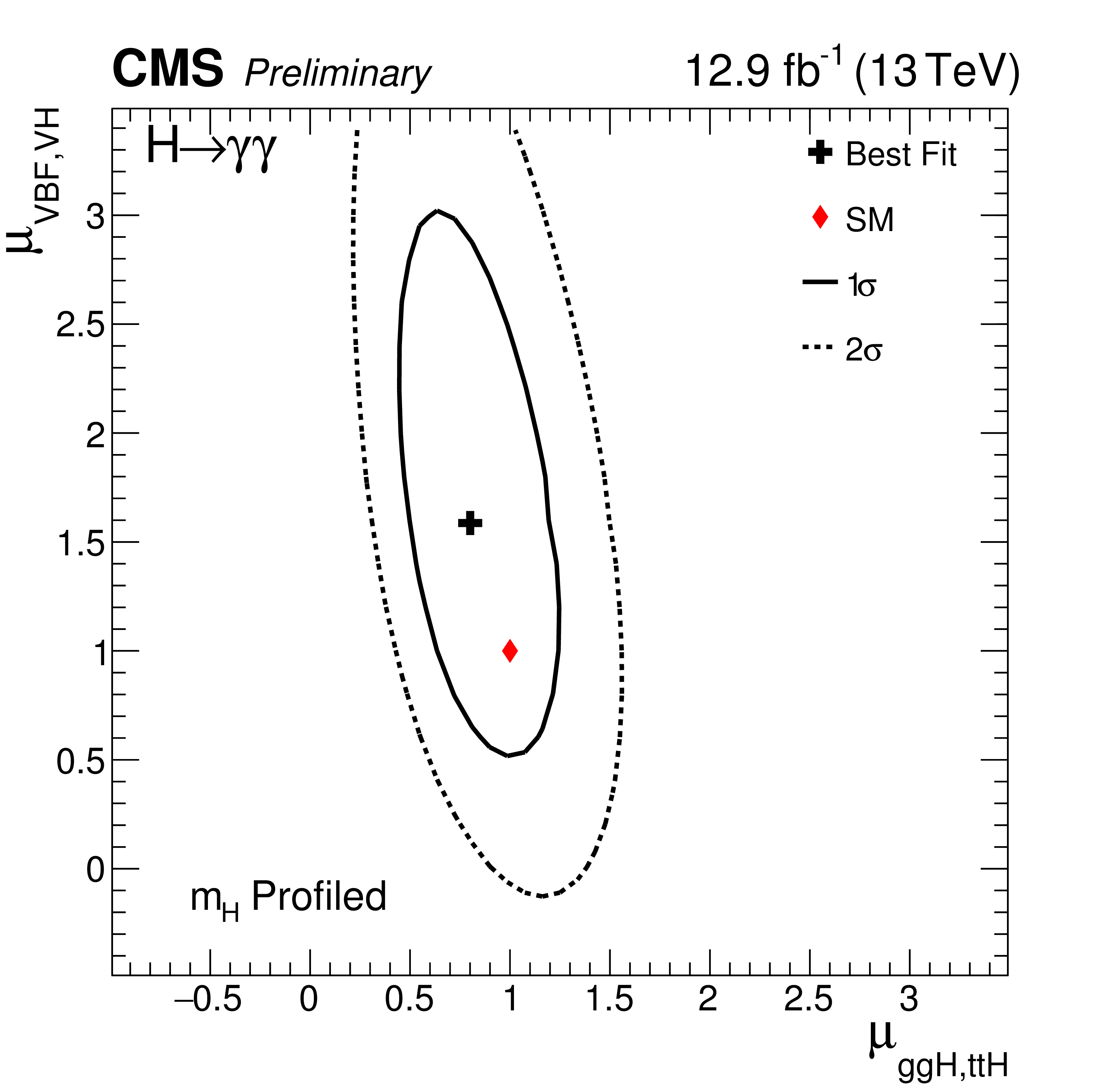
Figure 25:
The two-dimensional best-fit (black cross) of the signal strengths for fermionic (ggH, $\mathrm {t\bar{t}H}$) and bosonic (VBF, ZH, WH) production modes compared to the SM expectations (red diamond). The Higgs boson mass is profiled in the fit. The solid (dashed) line represents the 1 standard deviation (2 standard deviation) confidence region. The axis ranges have been chosen to be exactly the same as those from the equivalent plot from Run 1 (Fig.23 in [9]). |
png pdf |
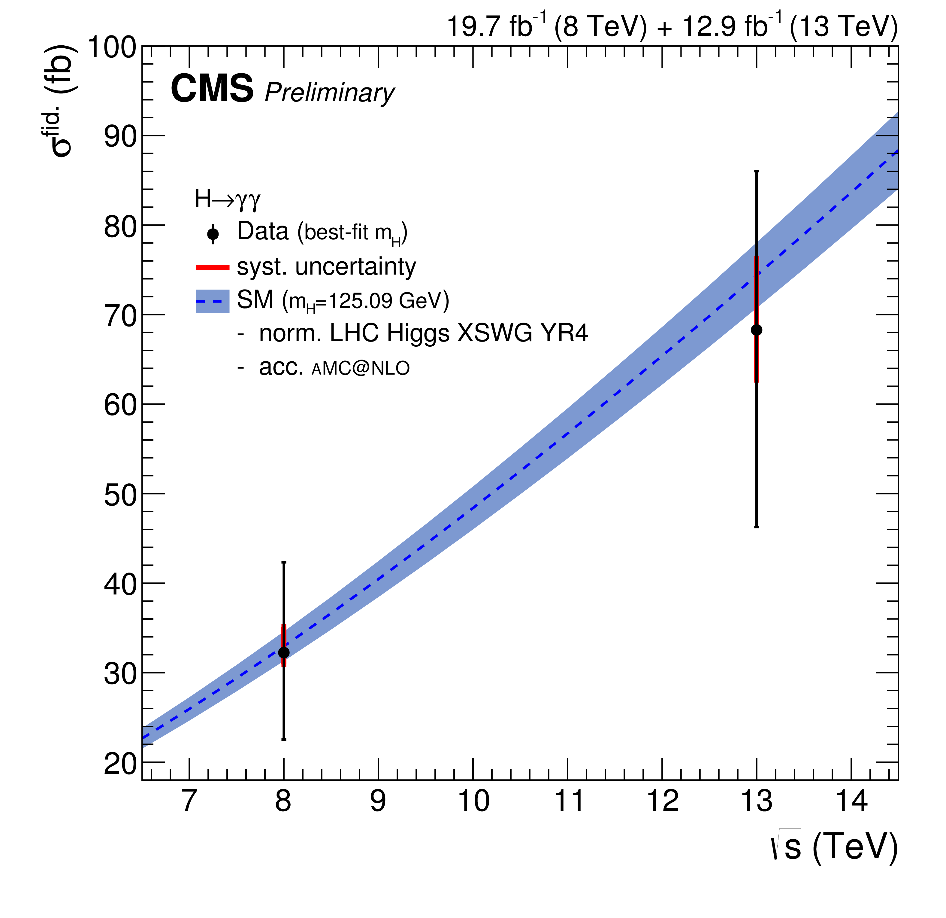
Figure 26:
The results of the measurements of the fiducial cross section by CMS at 8TeV (from the Run 1 analysis [9]) and (13TeV from this analysis) are shown. The black markers represent the best-fit value of the fiducial cross section for the best-fit mass in each case, along with the corresponding uncertainties. The red lines represent the size of the systematic component on the uncertainty. The blue dashed line and shading represent the SM expected fiducial cross section and uncertainty for a Higgs boson of mass $m_{\mathrm{H}}=125.09$ GeV. The normalisation has been set using the latest values from [18] and the acceptance is defined using the aMC@NLO generator-level quantities in both cases. |
| Tables | |

png pdf |
Table 1:
Preselection requirements. |

png pdf |
Table 2:
Photon preselection efficiencies measured in four photon categories, obtained with a tag and probe technique using Z$\rightarrow $ e$^{+}$e$^{-}$ events after applying all requirements except the electron veto. |

png pdf |
Table 3:
The expected number of signal events per category and the percentage breakdown per production mode in that category. The $\sigma _{eff}$, computed as the smallest interval containing 68.3% of the invariant mass distribution, and $\sigma _{HM}$, computed as the width of the distribution at half of its highest point divided by 2.35 are also shown as an estimate of the $m_{\gamma \gamma }$ resolution in that category. The expected number of background events per GeV around 125 GeV is also listed. |
| Summary |
| We report the observation of the Higgs boson decaying in the diphoton channel and the measurement of some of its properties. The analysis uses the 2016 dataset so far collected by the CMS experiment in proton-proton collisions at $\sqrt{s}=$ 13 TeV. The analysis follows closely the strategy adopted for the Run 1 result [9]. The selected events are divided into classes loosely targeting the different Higgs production processes, in order to increase the overall sensitivity of the analysis. A separate analysis making a measurement of the fiducial cross-section of the Higgs boson is also reported. A clear signal is observed in the diphoton channel. The significance of the observation at the Run 1 best fit mass of $m_{\mathrm{H}} =$ 125.09 GeV is 5. $\sigma$ where 6.2$ \sigma$ was expected for the SM Higgs boson, and the best-fit signal strength fixing $m_{\mathrm{H}} =$ 125.09 GeV is reported to be 0.91 $\pm$ 0.20 = 0.91 $\pm$ 0.17 (stat) $^{+0.09}_{-0.07}$ (syst) $^{+0.08}_{-0.05}$ (theo). The best-fit values for the signal strength modifiers associated with the ggH and ttH production mechanisms, and with the VBF and VH mechanisms are found to be $\mu_{ggH,t\bar{t}H} =$ 0.80 $^{+0.14}_{-0.18}$ and $\mu_{VBF,VH}=$ 1.59 $^{+0.73}_{-0.45}$ respectively when $m_{\mathrm{H}}$ is profiled in the fit. The highest significance of 6.1$ \sigma$ was observed at $m_{\mathrm{H}} =$ 126.0 GeV, where 6.2$ \sigma$ was expected. The best-fit value of the fiducial cross section of the Higgs boson is found to be $\hat{\sigma}_{fid} =$ 69 $^{+18}_{-22}$ fb = 69 $^{+16}_{-22}$ (stat) $^{+8} _{-6}$ (syst) fb, where the standard model theoretical prediction is 73.8 $\pm$ 3.8 fb. All the results are compatible with the expectations from a standard model Higgs boson. |
| References | ||||
| 1 | S. L. Glashow | Partial-symmetries of weak interactions | Nucl. Phys. 22 (1961) 579 | |
| 2 | S. Weinberg | A model of leptons | PRL 19 (1967) 1264 | |
| 3 | A. Salam | Weak and electromagnetic interactions | in Elementary particle physics: relativistic groups and analyticity, N. Svartholm, ed., p. 367 Almquvist \& Wiskell, 1968 Proceedings of the eighth Nobel symposium | |
| 4 | ATLAS Collaboration | Observation of a new particle in the search for the Standard Model Higgs boson with the ATLAS detector at the LHC | PLB716 (2012) 1--29 | 1207.7214 |
| 5 | CMS Collaboration | Observation of a new boson at a mass of 125 GeV with the CMS experiment at the LHC | PLB716 (2012) 30--61 | CMS-HIG-12-028 1207.7235 |
| 6 | F. Englert and R. Brout | Broken symmetries and the masses of gauge bosons | PRL 13 (1964) 321 | |
| 7 | P. W. Higgs | Broken symmetry and the mass of gauge vector mesons | PRL 13 (1964) 508 | |
| 8 | G. Guralnik, C. Hagen, and T. Kibble | Global Conservation Laws and Massless Particles | Phys.Rev.Lett. 13 (1964) 585 | |
| 9 | CMS Collaboration | Observation of the diphoton decay of the Higgs boson and measurement of its properties | EPJC74 (2014), no. 10 | CMS-HIG-13-001 1407.0558 |
| 10 | ATLAS, CMS Collaboration | Combined Measurement of the Higgs Boson Mass in $ pp $ Collisions at $ \sqrt{s}=7 $ and 8 TeV with the ATLAS and CMS Experiments | PRL 114 (2015) 191803 | 1503.07589 |
| 11 | CMS Collaboration | First results on Higgs to gammagamma at 13 TeV | CMS-PAS-HIG-15-005 | CMS-PAS-HIG-15-005 |
| 12 | CMS Collaboration | The CMS experiment at the CERN LHC | JINST 3 (2008) S08004 | CMS-00-001 |
| 13 | CMS Collaboration | Performance of Photon Reconstruction and Identification with the CMS Detector in Proton-Proton Collisions at sqrt(s) = 8 TeV | JINST 10 (2015), no. 08, P08010 | CMS-EGM-14-001 1502.02702 |
| 14 | J. Alwall et al. | The automated computation of tree-level and next-to-leading order differential cross sections, and their matching to parton shower simulations | JHEP 07 (2014) 079 | 1405.0301 |
| 15 | T. Sjostrand, S. Mrenna, and P. Z. Skands | A Brief Introduction to PYTHIA 8.1 | CPC 178 (2008) 852--867 | 0710.3820 |
| 16 | R. Frederix and S. Frixione | Merging meets matching in MC@NLO | JHEP 12 (2012) 061 | 1209.6215 |
| 17 | CMS Collaboration | Event generator tunes obtained from underlying event and multiparton scattering measurements | CMS-GEN-14-001 1512.00815 |
|
| 18 | LHC Higgs Cross Section Working Group Collaboration | Handbook of LHC Higgs Cross Sections: 4. Higgs Properties | technical report | |
| 19 | T. Gleisberg et al. | Event generation with SHERPA 1.1 | JHEP 02 (2009) 007 | 0811.4622 |
| 20 | GEANT4 Collaboration | GEANT4: A Simulation toolkit | NIMA 506 (2003) 250 | |
| 21 | CMS Collaboration | Particle-Flow Event Reconstruction in CMS and Performance for Jets, Taus, and MET | CDS | |
| 22 | M. Cacciari, G. P. Salam, and G. Soyez | The anti-$ k_t $ jet clustering algorithm | JHEP 04 (2008) 063 | |
| 23 | M. Cacciari, G. P. Salam, and G. Soyez | FastJet User Manual | EPJC72 (2012) 1896 | 1111.6097 |
| 24 | CMS Collaboration | Determination of Jet Energy Calibration and Transverse Momentum Resolution in CMS | JINST 06 (2011) P11002 | |
| 25 | M. Cacciari and G. P. Salam | Pileup subtraction using jet areas | PLB659 (2008) 119 | |
| 26 | CMS Collaboration | Measurement of the inclusive W and Z production cross sections in pp collisions at $ \sqrt {s} = 7 $ TeV with the CMS experiment | JHEP 2011 (2011) 1 | |
| 27 | CMS Collaboration | Electron and Photon performance using data collected by CMS at $ \sqrt{s} $ = 13 TeV and 25ns | CDS | |
| 28 | CMS Collaboration | Identification of b-quark jets with the CMS experiment | JINST 8 (2013) P04013 | CMS-BTV-12-001 1211.4462 |
| 29 | D. L. Rainwater, R. Szalapski, and D. Zeppenfeld | Probing color singlet exchange in $ Z $ + two jet events at the CERN LHC | PRD54 (1996) 6680--6689 | hep-ph/9605444 |
| 30 | G. Cowan et al. | Asymptotic formulae for likelihood-based tests of new physics | EPJC 71 (2011) 1 | 1007.1727 |
| 31 | P. D. Dauncey, M. Kenzie, N. Wardle, and G. J. Davies | Handling uncertainties in background shapes: the discrete profiling method | JINST 10 (2015), no. 04, P04015 | 1408.6865 |
| 32 | J. Butterworth et al. | PDF4LHC recommendations for LHC Run II | JPG43 (2016) 023001 | 1510.03865 |
| 33 | F. Demartin et al. | The impact of PDF and alphas uncertainties on Higgs Production in gluon fusion at hadron colliders | PRD82 (2010) 014002 | 1004.0962 |
| 34 | S. Carrazza et al. | An Unbiased Hessian Representation for Monte Carlo PDFs | EPJC75 (2015), no. 8, 369 | 1505.06736 |
| 35 | CMS Collaboration | First measurement of the differential cross section for $ \mathrm{ t \bar{t} } $ production in the dilepton final state at $ \sqrt{s}=13 $~TeV | Technical Report CMS-PAS-TOP-15-010, CERN, 2015. Geneva, Dec | |
| 36 | LHC Higgs Cross Section Working Group Collaboration | Handbook of LHC Higgs Cross Sections: 3. Higgs Properties | 1307.1347 | |
|
|
Compact Muon Solenoid LHC, CERN |
|

|

|

|

|

|