

Compact Muon Solenoid
LHC, CERN
| CMS-PAS-SUS-16-012 | ||
| Search for supersymmetry in events with a Higgs decaying to two photons using the razor variables | ||
| CMS Collaboration | ||
| August 2016 | ||
| Abstract: A search for supersymmetry is carried out in proton-proton collisions with a center of mass energy of 13 TeV and corresponding to an integrated luminosity of 15.2 $\mathrm{fb}^{-1}$ collected with the CMS experiment at the CERN LHC. Events are selected by requiring one Higgs boson candidate decaying into two photons in association with at least one jet. Events are categorized according to the properties of the Higgs boson candidate(s) and the razor variables ($M_{R}$ and $R^{2}$) are used to improve discrimination between SUSY signals and the standard model backgrounds. The search is carried out by fitting the diphoton invariant mass distribution in each search region. The result of the search is interpreted in the context of a simplified model of bottom squark production and upper limits on the corresponding production cross section are derived. | ||
| Links: CDS record (PDF) ; inSPIRE record ; CADI line (restricted) ; | ||
| Figures | |

png pdf |
Figure 1:
Diagram illustrating the SUSY benchmark simplified model of bottom squark decays to a Higgs boson, a b-jet, and the LSP. |
png pdf |
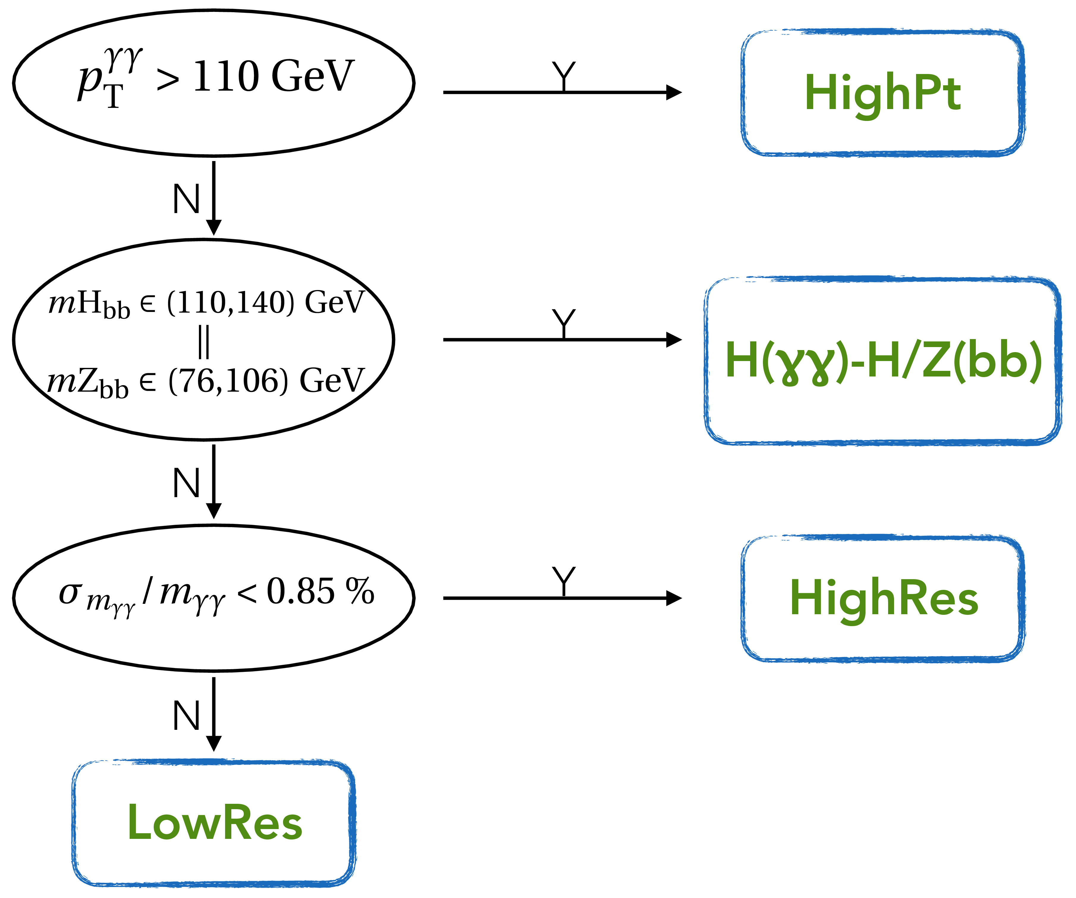
Figure 2:
Diagram illustrating the event categorization used in the analysis. |
png pdf |
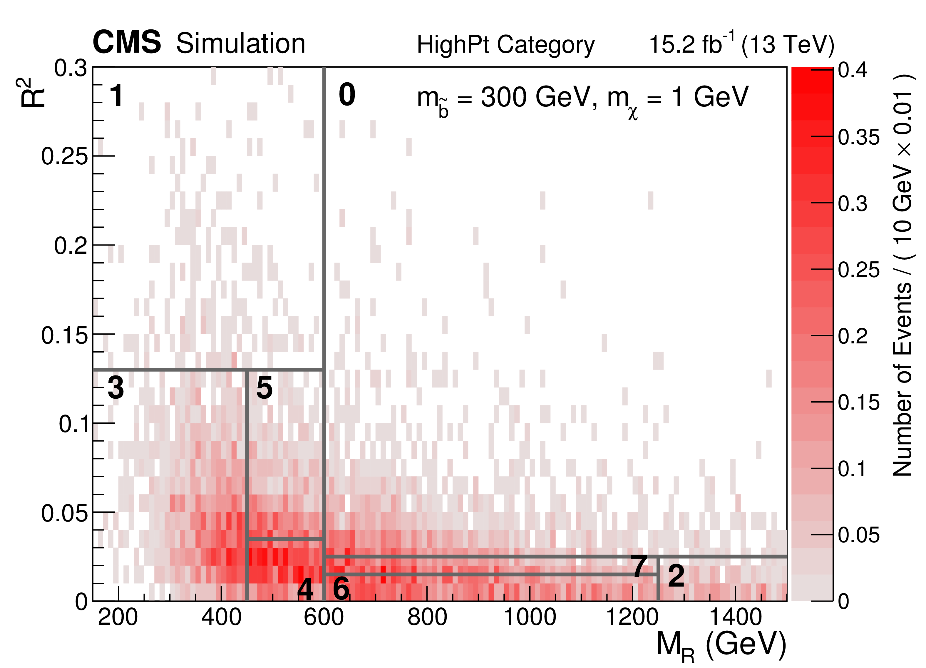
Figure 3-a:
Distribution of events in the $M_{R}$ and $R^{2}$ plane for the HighPt and H($\gamma \gamma $)-H/Z(bb) category for sbottom pair production with $m_{\tilde{b}}=$ 300 GeV and $m_{\chi }=$ 1 GeV. The signal expectation is shown in the color scale and the bin numbers show where each bin is located in the $M_{R}$ and $R^{2}$ plane. |

png pdf |
Figure 3-b:
Distribution of events in the $M_{R}$ and $R^{2}$ plane for the HighPt and H($\gamma \gamma $)-H/Z(bb) category for sbottom pair production with $m_{\tilde{b}}=$ 300 GeV and $m_{\chi }=$ 1 GeV. The signal expectation is shown in the color scale and the bin numbers show where each bin is located in the $M_{R}$ and $R^{2}$ plane. |
png pdf |
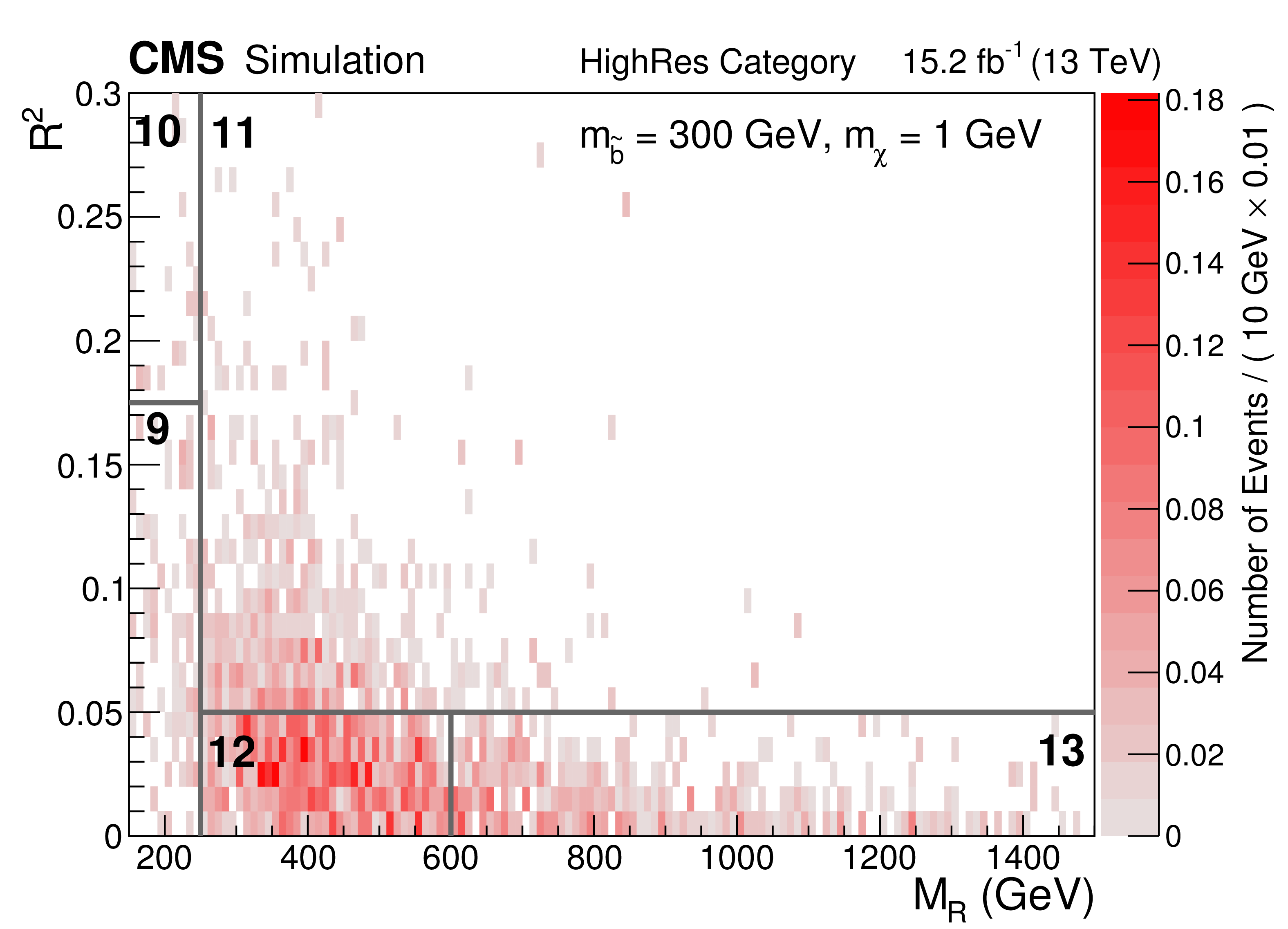
Figure 4-a:
Distribution of events in the $M_{R}$ and $R^{2}$ plane for the HighRes and LowRes categories for sbottom pair production with $m_{\tilde{b}}=$ 300 GeV and $m_{\chi }=$ 1 GeV. The signal expectation is shown in the color scale and the bin numbers show where each bin is located in the $M_{R}$ and $R^{2}$ plane. |
png pdf |
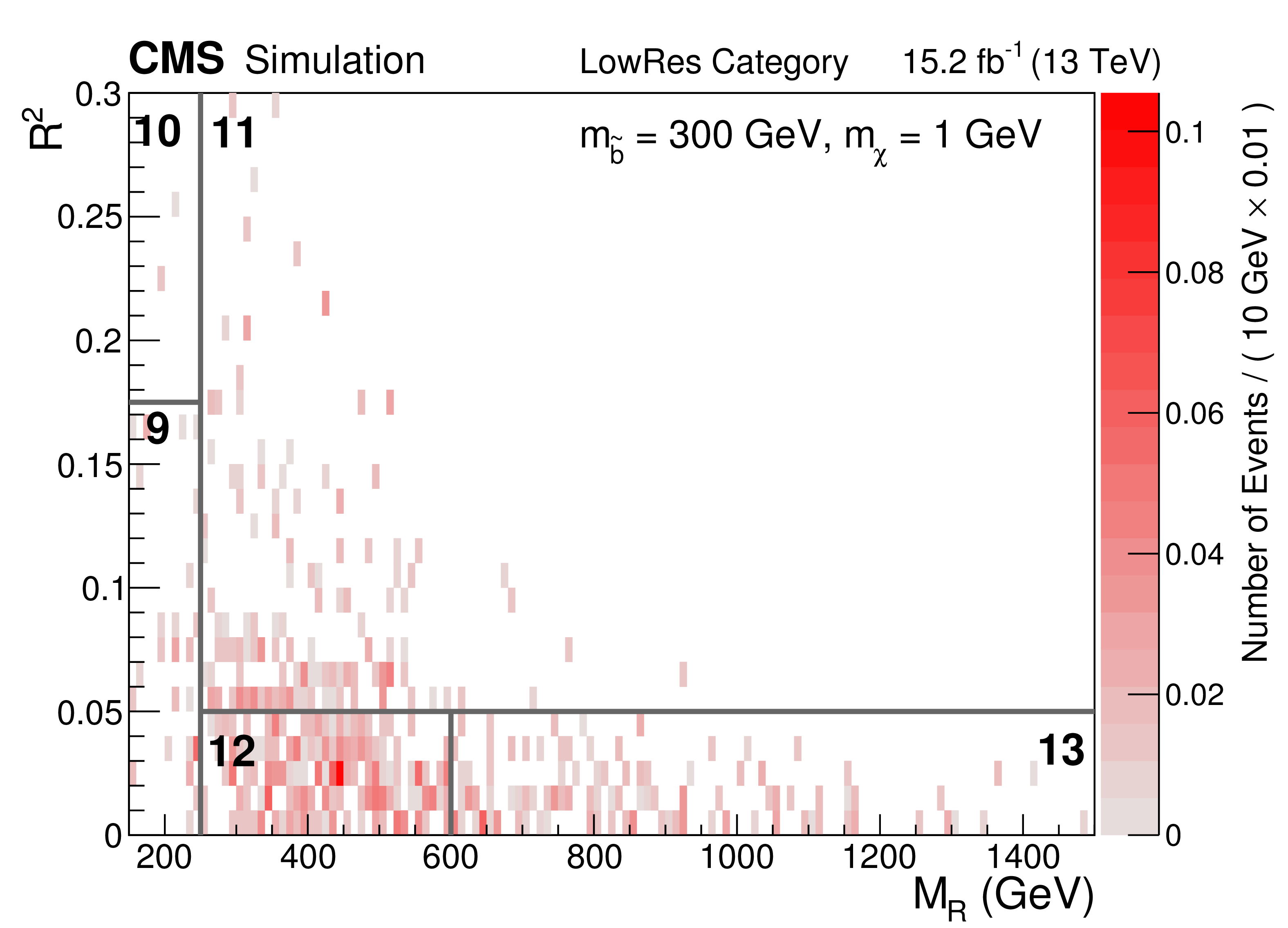
Figure 4-b:
Distribution of events in the $M_{R}$ and $R^{2}$ plane for the HighRes and LowRes categories for sbottom pair production with $m_{\tilde{b}}=$ 300 GeV and $m_{\chi }=$ 1 GeV. The signal expectation is shown in the color scale and the bin numbers show where each bin is located in the $M_{R}$ and $R^{2}$ plane. |
png |
Figure 5-a:
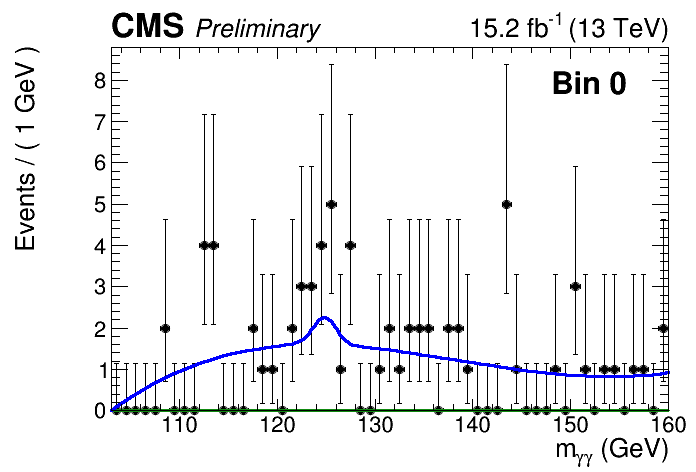
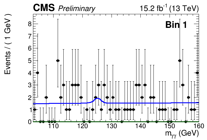
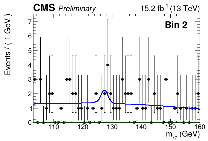
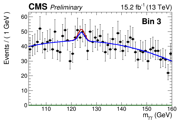
The diphoton mass distribution for various search region bins in the HighPt category are shown along with the background-only fit (a,c,e) and the signal plus background fit (b,d,f). The red curve represents the background prediction; the green curve represents the signal; and the blue curve represents the sum of the signal and background. The definition of the search bin is labeled above each pair of plots. |

png |
Figure 5-b:
The diphoton mass distribution for various search region bins in the HighPt category are shown along with the background-only fit (a,c,e) and the signal plus background fit (b,d,f). The red curve represents the background prediction; the green curve represents the signal; and the blue curve represents the sum of the signal and background. The definition of the search bin is labeled above each pair of plots. |
png |
Figure 5-c:
The diphoton mass distribution for various search region bins in the HighPt category are shown along with the background-only fit (a,c,e) and the signal plus background fit (b,d,f). The red curve represents the background prediction; the green curve represents the signal; and the blue curve represents the sum of the signal and background. The definition of the search bin is labeled above each pair of plots. |

png |
Figure 5-d:
The diphoton mass distribution for various search region bins in the HighPt category are shown along with the background-only fit (a,c,e) and the signal plus background fit (b,d,f). The red curve represents the background prediction; the green curve represents the signal; and the blue curve represents the sum of the signal and background. The definition of the search bin is labeled above each pair of plots. |
png |
Figure 5-e:
The diphoton mass distribution for various search region bins in the HighPt category are shown along with the background-only fit (a,c,e) and the signal plus background fit (b,d,f). The red curve represents the background prediction; the green curve represents the signal; and the blue curve represents the sum of the signal and background. The definition of the search bin is labeled above each pair of plots. |

png |
Figure 5-f:
The diphoton mass distribution for various search region bins in the HighPt category are shown along with the background-only fit (a,c,e) and the signal plus background fit (b,d,f). The red curve represents the background prediction; the green curve represents the signal; and the blue curve represents the sum of the signal and background. The definition of the search bin is labeled above each pair of plots. |

png |
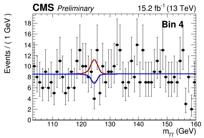
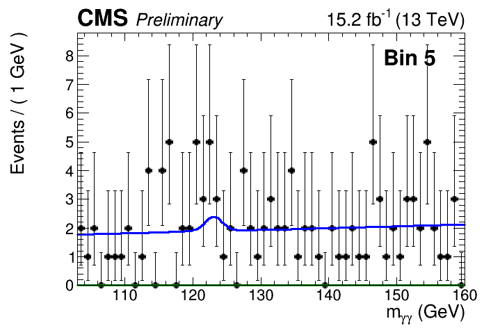
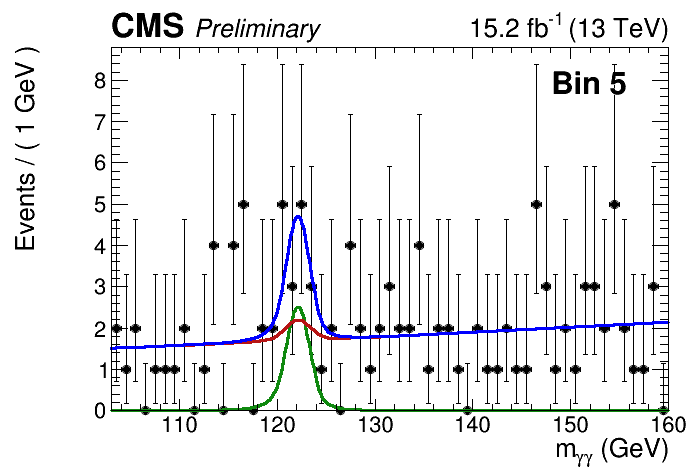
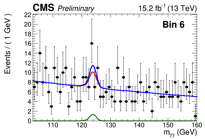
Figure 6-a:
The diphoton mass distribution for various search region bins in the HighPt category are shown along with the background-only fit (a,c,e) and the signal plus background fit (b,d,f). The red curve represents the background prediction; the green curve represents the signal; and the blue curve represents the sum of the signal and background. The definition of the bin is labeled above each pair of plots. |
png |
Figure 6-b:
The diphoton mass distribution for various search region bins in the HighPt category are shown along with the background-only fit (a,c,e) and the signal plus background fit (b,d,f). The red curve represents the background prediction; the green curve represents the signal; and the blue curve represents the sum of the signal and background. The definition of the bin is labeled above each pair of plots. |

png |
Figure 6-c:
The diphoton mass distribution for various search region bins in the HighPt category are shown along with the background-only fit (a,c,e) and the signal plus background fit (b,d,f). The red curve represents the background prediction; the green curve represents the signal; and the blue curve represents the sum of the signal and background. The definition of the bin is labeled above each pair of plots. |
png |
Figure 6-d:
The diphoton mass distribution for various search region bins in the HighPt category are shown along with the background-only fit (a,c,e) and the signal plus background fit (b,d,f). The red curve represents the background prediction; the green curve represents the signal; and the blue curve represents the sum of the signal and background. The definition of the bin is labeled above each pair of plots. |
png |
Figure 6-e:
The diphoton mass distribution for various search region bins in the HighPt category are shown along with the background-only fit (a,c,e) and the signal plus background fit (b,d,f). The red curve represents the background prediction; the green curve represents the signal; and the blue curve represents the sum of the signal and background. The definition of the bin is labeled above each pair of plots. |
png |
Figure 6-f:
The diphoton mass distribution for various search region bins in the HighPt category are shown along with the background-only fit (a,c,e) and the signal plus background fit (b,d,f). The red curve represents the background prediction; the green curve represents the signal; and the blue curve represents the sum of the signal and background. The definition of the bin is labeled above each pair of plots. |

png |
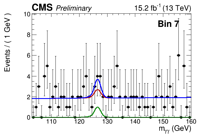
Figure 7-a:
The diphoton mass distribution for various search region bins in the HighPt category are shown along with the background-only fit (a,c) and the signal plus background fit (b,d). The red curve represents the background prediction; the green curve represents the signal; and the blue curve represents the sum of the signal and background. The definition of the bin is labeled above each pair of plots. |
png |
Figure 7-b:
The diphoton mass distribution for various search region bins in the HighPt category are shown along with the background-only fit (a,c) and the signal plus background fit (b,d). The red curve represents the background prediction; the green curve represents the signal; and the blue curve represents the sum of the signal and background. The definition of the bin is labeled above each pair of plots. |

png |
Figure 7-c:
The diphoton mass distribution for various search region bins in the HighPt category are shown along with the background-only fit (a,c) and the signal plus background fit (b,d). The red curve represents the background prediction; the green curve represents the signal; and the blue curve represents the sum of the signal and background. The definition of the bin is labeled above each pair of plots. |
png |
Figure 7-d:
The diphoton mass distribution for various search region bins in the HighPt category are shown along with the background-only fit (a,c) and the signal plus background fit (b,d). The red curve represents the background prediction; the green curve represents the signal; and the blue curve represents the sum of the signal and background. The definition of the bin is labeled above each pair of plots. |
png |
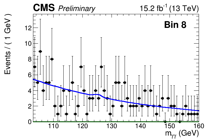
Figure 8-a:
The diphoton mass distribution for various search region bins in the H($\gamma \gamma $)-H/Z(bb) category are shown along with the background-only fit (a) and the signal plus background fit (b). The red curve represents the background prediction; the green curve represents the signal; and the blue curve represents the sum of the signal and background. The definition of the bin is labeled above each pair of plots. |

png |
Figure 8-b:
The diphoton mass distribution for various search region bins in the H($\gamma \gamma $)-H/Z(bb) category are shown along with the background-only fit (a) and the signal plus background fit (b). The red curve represents the background prediction; the green curve represents the signal; and the blue curve represents the sum of the signal and background. The definition of the bin is labeled above each pair of plots. |

png |
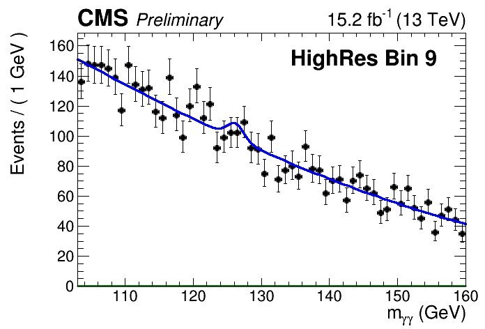
Figure 9-a:
The diphoton mass distribution for the search region bin 9 are shown along with the background-only fit (a,c) and the signal plus background fit (b,d). The top row shows the HighRes category, while the bottom row shows the LowRes category. The red curve represents the background prediction; the green curve represents the signal; and the blue curve represents the sum of the signal and background. The definition of the bin is labeled above each pair of plots. |
png |
Figure 9-b:
The diphoton mass distribution for the search region bin 9 are shown along with the background-only fit (a,c) and the signal plus background fit (b,d). The top row shows the HighRes category, while the bottom row shows the LowRes category. The red curve represents the background prediction; the green curve represents the signal; and the blue curve represents the sum of the signal and background. The definition of the bin is labeled above each pair of plots. |

png |
Figure 9-c:
The diphoton mass distribution for the search region bin 9 are shown along with the background-only fit (a,c) and the signal plus background fit (b,d). The top row shows the HighRes category, while the bottom row shows the LowRes category. The red curve represents the background prediction; the green curve represents the signal; and the blue curve represents the sum of the signal and background. The definition of the bin is labeled above each pair of plots. |

png |
Figure 9-d:
The diphoton mass distribution for the search region bin 9 are shown along with the background-only fit (a,c) and the signal plus background fit (b,d). The top row shows the HighRes category, while the bottom row shows the LowRes category. The red curve represents the background prediction; the green curve represents the signal; and the blue curve represents the sum of the signal and background. The definition of the bin is labeled above each pair of plots. |
png |
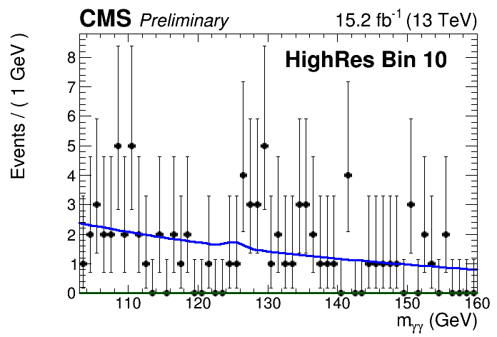
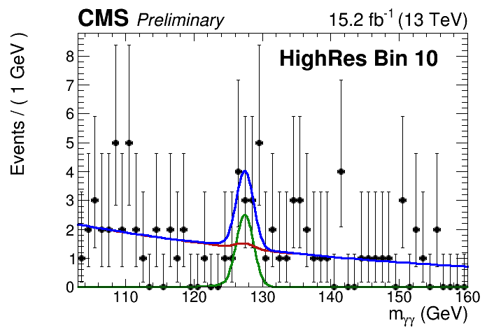
Figure 10-a:
The diphoton mass distribution for the search region bin 10 are shown along with the background-only fit (a,c) and the signal plus background fit (b,d). The top row shows the HighRes category, while the bottom row shows the LowRes category. The red curve represents the background prediction; the green curve represents the signal; and the blue curve represents the sum of the signal and background. The definition of the bin is labeled above each pair of plots. |
png |
Figure 10-b:
The diphoton mass distribution for the search region bin 10 are shown along with the background-only fit (a,c) and the signal plus background fit (b,d). The top row shows the HighRes category, while the bottom row shows the LowRes category. The red curve represents the background prediction; the green curve represents the signal; and the blue curve represents the sum of the signal and background. The definition of the bin is labeled above each pair of plots. |

png |
Figure 10-c:
The diphoton mass distribution for the search region bin 10 are shown along with the background-only fit (a,c) and the signal plus background fit (b,d). The top row shows the HighRes category, while the bottom row shows the LowRes category. The red curve represents the background prediction; the green curve represents the signal; and the blue curve represents the sum of the signal and background. The definition of the bin is labeled above each pair of plots. |

png |
Figure 10-d:
The diphoton mass distribution for the search region bin 10 are shown along with the background-only fit (a,c) and the signal plus background fit (b,d). The top row shows the HighRes category, while the bottom row shows the LowRes category. The red curve represents the background prediction; the green curve represents the signal; and the blue curve represents the sum of the signal and background. The definition of the bin is labeled above each pair of plots. |
png |
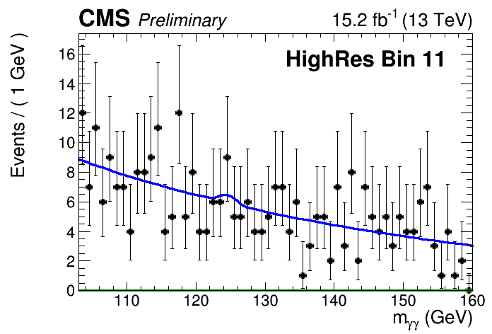
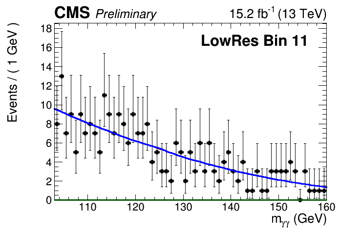
Figure 11-a:
The diphoton mass distribution for the search region bin 11 are shown along with the background-only fit (a,c) and the signal plus background fit (b,d). The top row shows the HighRes category, while the bottom row shows the LowRes category. The red curve represents the background prediction; the green curve represents the signal; and the blue curve represents the sum of the signal and background. The definition of the bin is labeled above each pair of plots. |

png |
Figure 11-b:
The diphoton mass distribution for the search region bin 11 are shown along with the background-only fit (a,c) and the signal plus background fit (b,d). The top row shows the HighRes category, while the bottom row shows the LowRes category. The red curve represents the background prediction; the green curve represents the signal; and the blue curve represents the sum of the signal and background. The definition of the bin is labeled above each pair of plots. |

png |
Figure 11-c:
The diphoton mass distribution for the search region bin 11 are shown along with the background-only fit (a,c) and the signal plus background fit (b,d). The top row shows the HighRes category, while the bottom row shows the LowRes category. The red curve represents the background prediction; the green curve represents the signal; and the blue curve represents the sum of the signal and background. The definition of the bin is labeled above each pair of plots. |
png |
Figure 11-d:
The diphoton mass distribution for the search region bin 11 are shown along with the background-only fit (a,c) and the signal plus background fit (b,d). The top row shows the HighRes category, while the bottom row shows the LowRes category. The red curve represents the background prediction; the green curve represents the signal; and the blue curve represents the sum of the signal and background. The definition of the bin is labeled above each pair of plots. |
png |
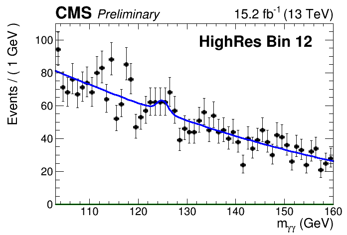
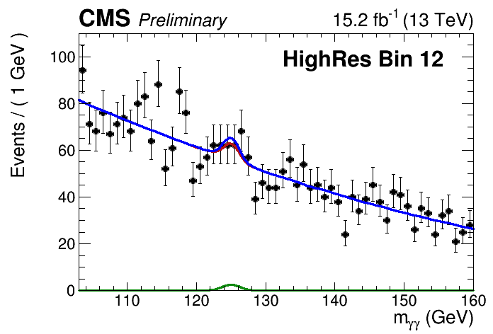
Figure 12-a:
The diphoton mass distribution for the search region bin 12 are shown along with the background-only fit (a,c) and the signal plus background fit (b,d). The top row shows the HighRes category, while the bottom row shows the LowRes category. The red curve represents the background prediction; the green curve represents the signal; and the blue curve represents the sum of the signal and background. The definition of the bin is labeled above each pair of plots. |
png |
Figure 12-b:
The diphoton mass distribution for the search region bin 12 are shown along with the background-only fit (a,c) and the signal plus background fit (b,d). The top row shows the HighRes category, while the bottom row shows the LowRes category. The red curve represents the background prediction; the green curve represents the signal; and the blue curve represents the sum of the signal and background. The definition of the bin is labeled above each pair of plots. |

png |
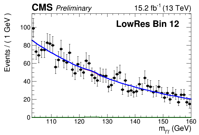
Figure 12-c:
The diphoton mass distribution for the search region bin 12 are shown along with the background-only fit (a,c) and the signal plus background fit (b,d). The top row shows the HighRes category, while the bottom row shows the LowRes category. The red curve represents the background prediction; the green curve represents the signal; and the blue curve represents the sum of the signal and background. The definition of the bin is labeled above each pair of plots. |
png |
Figure 12-d:
The diphoton mass distribution for the search region bin 12 are shown along with the background-only fit (a,c) and the signal plus background fit (b,d). The top row shows the HighRes category, while the bottom row shows the LowRes category. The red curve represents the background prediction; the green curve represents the signal; and the blue curve represents the sum of the signal and background. The definition of the bin is labeled above each pair of plots. |

png |
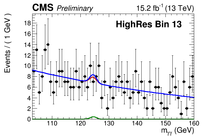
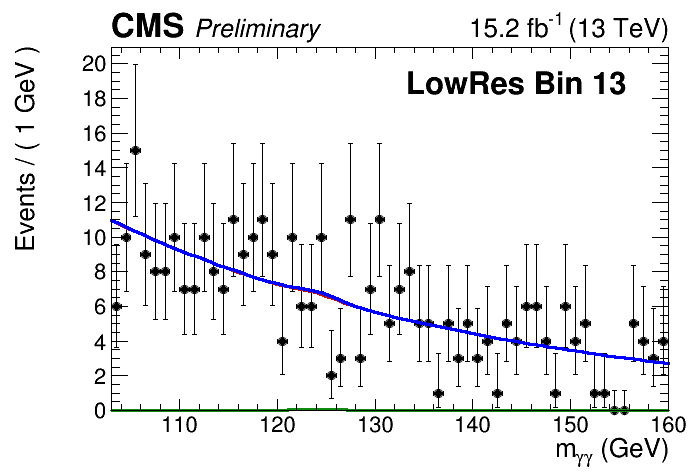
Figure 13-a:
The diphoton mass distribution for the search region bin 13 are shown along with the background-only fit (a,c) and the signal plus background fit (b,d). The top row shows the HighRes category, while the bottom row shows the LowRes category. The red curve represents the background prediction; the green curve represents the signal; and the blue curve represents the sum of the signal and background. The definition of the bin is labeled above each pair of plots. |
png |
Figure 13-b:
The diphoton mass distribution for the search region bin 13 are shown along with the background-only fit (a,c) and the signal plus background fit (b,d). The top row shows the HighRes category, while the bottom row shows the LowRes category. The red curve represents the background prediction; the green curve represents the signal; and the blue curve represents the sum of the signal and background. The definition of the bin is labeled above each pair of plots. |
png |
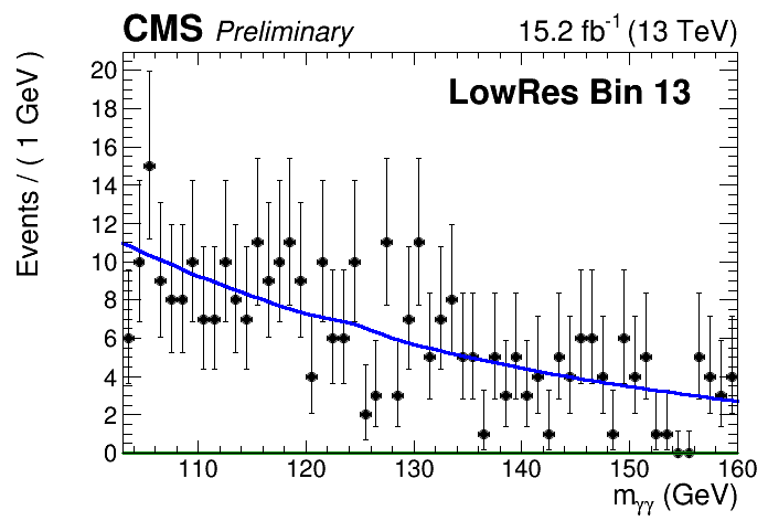
Figure 13-c:
The diphoton mass distribution for the search region bin 13 are shown along with the background-only fit (a,c) and the signal plus background fit (b,d). The top row shows the HighRes category, while the bottom row shows the LowRes category. The red curve represents the background prediction; the green curve represents the signal; and the blue curve represents the sum of the signal and background. The definition of the bin is labeled above each pair of plots. |
png |
Figure 13-d:
The diphoton mass distribution for the search region bin 13 are shown along with the background-only fit (a,c) and the signal plus background fit (b,d). The top row shows the HighRes category, while the bottom row shows the LowRes category. The red curve represents the background prediction; the green curve represents the signal; and the blue curve represents the sum of the signal and background. The definition of the bin is labeled above each pair of plots. |
png pdf |
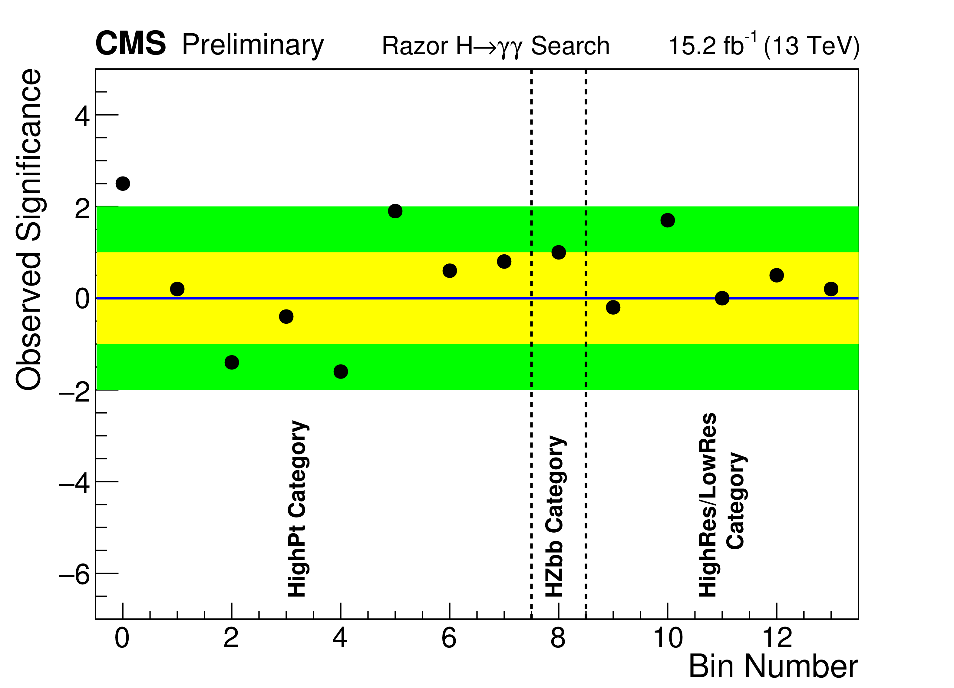
Figure 14:
The observed significance in units of standard deviations is plotted for each search bin. The significance is computed using the profile likelihood, where the sign reflects whether an excess (positive sign) or deficit (negative sign) is observed. The categories that the bins belong to are labeled at the bottom. The yellow and green bands represent the 1$\sigma $ and 2$\sigma $ regions, respectively. |
png pdf root |
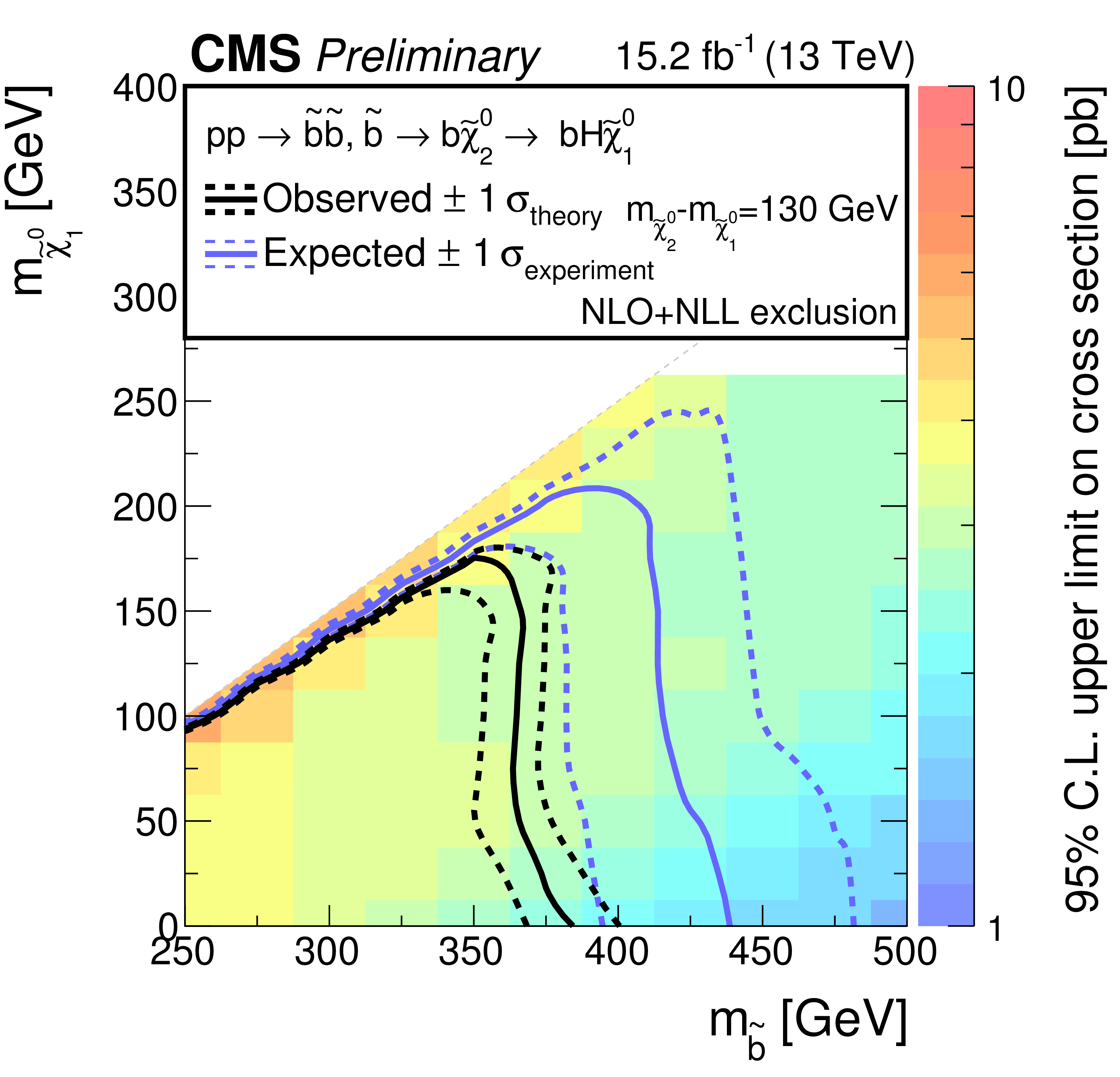
Figure 15:
The observed 95% confidence level (C.L.) upper limits on the production cross section for sbottom pair production decaying to a bottom quark, a Higgs boson, and the LSP are shown. The solid and dotted black contours represent the observed exclusion region and its 1$\sigma $ bands, while the analogous blue contours represent the expected exclusion region and its 1$\sigma $ bands. |
| Tables | |
png pdf |
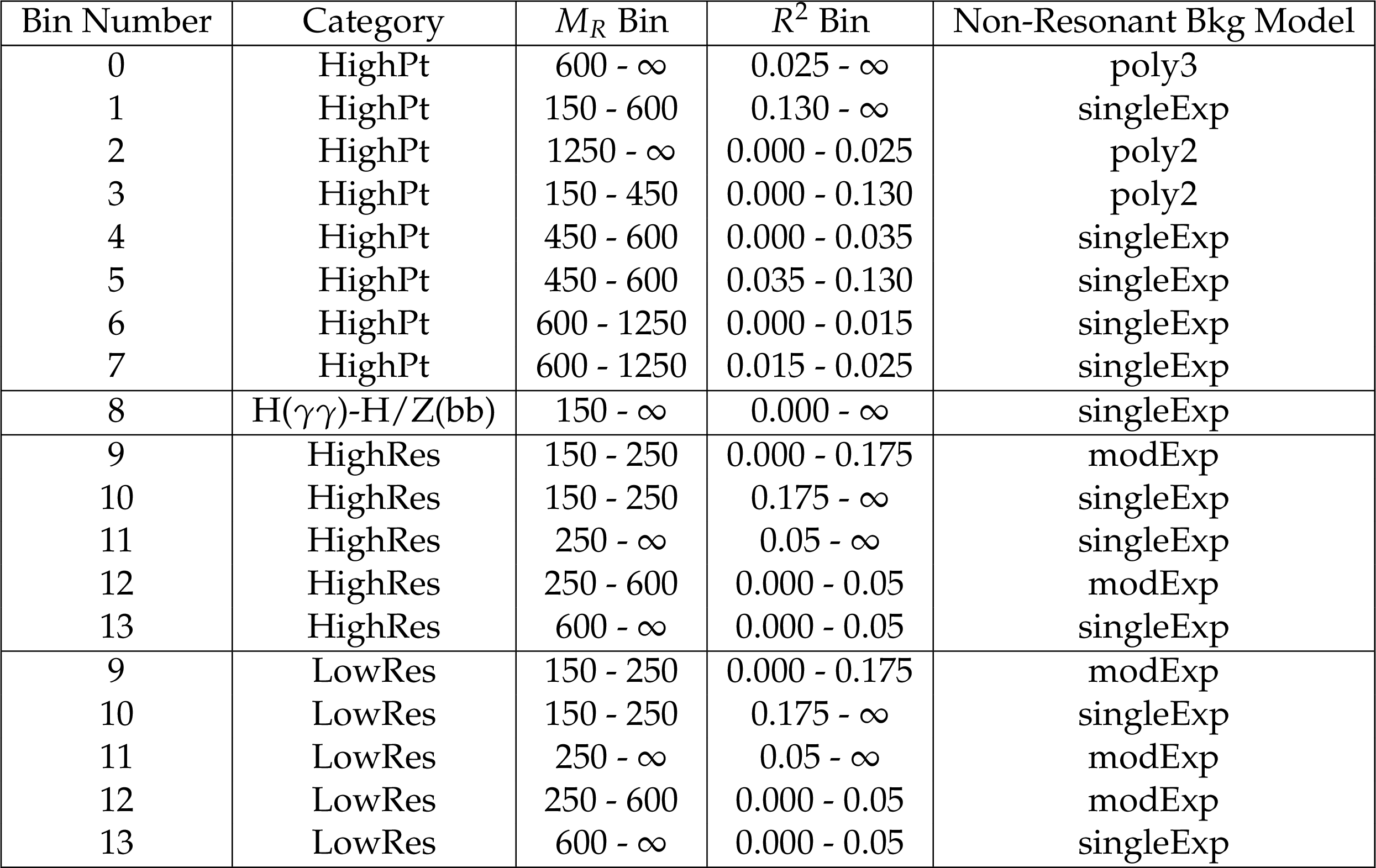
Table 1:
A summary of the search region bins in each category is presented. The functional form used to model the non-resonant background is also listed. An exponential function of the form $e^{-ax}$ is denoted as ``singleExp''; a modified exponential function of the form $e^{-ax^{b}}$ is denoted as ``modExp''; and an N'th order Bernstein polynomial is denoted by ``polyN''. |
png pdf |
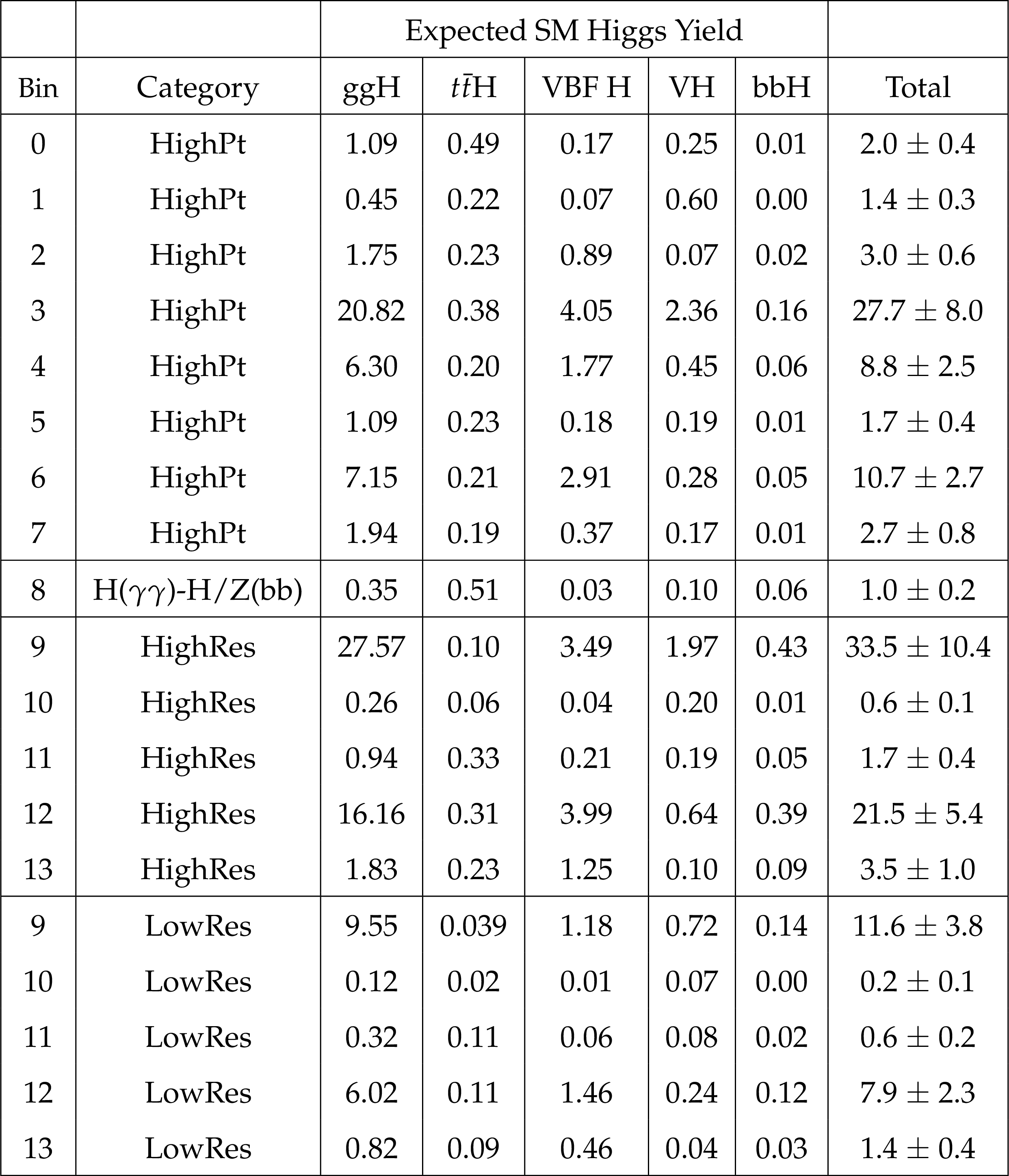
Table 2:
The predicted yields for the standard model Higgs background processes are shown for an integrated luminosity corresponding to 15.2 fb$^{-1}$ for each search region considered in this analysis. The contributions from each standard model Higgs process is shown separately, and the total is shown on the rightmost column along with its full uncertainty. |

png pdf |
Table 3:
Summary of systematic uncertainties and their size. |

png pdf |
Table 4:
The non-resonant background yields, SM Higgs background yields, best fit signal yields, and observed local significance are shown for the signal plus background fit in each search region bin. The uncertainties include both statistical and systematic components. The non-resonant background yields shown correspond to the yield within the window between 122 GeV and 129 GeV and is intended to better reflect the background under the signal peak. The observed significance for the bins in HighRes and LowRes categories are identical because they are the result of a simultaneous fit. The significance is computed using the profile likelihood, where the sign reflects whether an excess (positive sign) or deficit (negative sign) is observed. |
| Summary |
| A search for anomalous Higgs boson production through decays of supersymmetric particles is performed with data collected in 2015 and 2016 by the CMS experiment at the CERN LHC. Proton collisions collected at a center-of-mass energy $\sqrt{s}=$ 13 TeV are considered, corresponding to an integrated luminosity of about 15.2 fb$^{-1}$ (2.3 fb$^{-1}$ from 2015 and 12.9 fb$^{-1}$ from 2016). Higgs boson candidates are reconstructed from pairs of photons in the central part of the detector. The razor variables $M_{R}$ and $R^{2}$ are used to suppress SM Higgs boson production and other SM processes. The non-resonant background is estimated through a data-driven fit to the diphoton mass distribution using a functional form model selected by a combination of the AIC score and the result of a series of bias tests. The standard model Higgs background is estimated using the Monte Carlo simulation, with systematics on instrumental and theoretical uncertainties propagated. We interpret the results in terms of production cross-section limits on sbottom pair production each decaying to a Higgs boson, a b-quark, and the LSP, and exclude sbottoms with mass below 350 GeV. |
| References | ||||
| 1 | ATLAS Collaboration | Observation of a new particle in the search for the Standard Model Higgs boson with the ATLAS detector at the LHC | PLB 716 (2012) 1 | 1207.7214 |
| 2 | CMS Collaboration | Observation of a new boson at a mass of 125 GeV with the CMS experiment at the LHC | PLB 716 (2012) 30 | CMS-HIG-12-028 1207.7235 |
| 3 | CMS Collaboration | Inclusive search for squarks and gluinos in pp collisions at $ \sqrt{s} = 7 $ TeV | PRD 85 (2012) 012004 | CMS-SUS-10-009 1107.1279 |
| 4 | C. Rogan | Kinematics for new dynamics at the LHC | 1006.2727 | |
| 5 | CMS Collaboration | Search for SUSY with Higgs in the diphoton final state using the razor variables | CMS-PAS-SUS-14-017 | CMS-PAS-SUS-14-017 |
| 6 | C. Borschensky et al. | Squark and gluino production cross sections in pp collisions at $ \sqrt{s} $ = 13, 14, 33 and 100 TeV | EPJC74 (2014), no. 12 | 1407.5066 |
| 7 | CMS Collaboration | Observation of the diphoton decay of the Higgs boson and measurement of its properties | EPJC 74 (2014) 3076 | CMS-HIG-13-001 1407.0558 |
| 8 | CMS Collaboration | Performance of Photon Reconstruction and Identification with the CMS Detector in Proton-Proton Collisions at sqrt(s) = 8 TeV | JINST 10 (2015), no. 08, P08010 | CMS-EGM-14-001 1502.02702 |
| 9 | CMS Collaboration | Particle--flow event reconstruction in CMS and performance for jets, taus, and $ E_{\mathrm{T}}^{\text{miss}} $ | CDS | |
| 10 | CMS Collaboration | Commissioning of the particle-flow event reconstruction with the first LHC collisions recorded in the CMS detector | CDS | |
| 11 | M. Cacciari, G. P. Salam, and G. Soyez | FastJet user manual | EPJC 72 (2012) 1896 | 1111.6097 |
| 12 | M. Cacciari, G. P. Salam, and G. Soyez | The anti-k$ _{\mathrm T} $ jet clustering algorithm | JHEP 04 (2008) 063 | 0802.1189 |
| 13 | CMS Collaboration | Missing transverse energy performance of the CMS detector | JINST 6 (2011) P09001 | CMS-JME-10-009 1106.5048 |
| 14 | CMS Collaboration | Search for New Physics in the Multijet and Missing Transverse Momentum Final State in Proton-Proton Collisions at $ \sqrt{s} = 7 $ TeV | PRL 109 (2012) 171803 | CMS-SUS-12-011 1207.1898 |
| 15 | CMS Collaboration | Performance of the missing transverse energy reconstruction by the CMS experiment in $ \sqrt{s} $ = 8 TeV pp data | CDS | |
| 16 | CMS Collaboration | Performance of $ \mathrm{b } $ tagging at $ \sqrt{s} = $ 8 TeV in multijet, $ \mathrm{ t \bar{t} } $ and boosted topology events | CMS-PAS-BTV-13-001 | CMS-PAS-BTV-13-001 |
| 17 | CMS Collaboration | Search for supersymmetry with razor variables in pp collisions at $ \sqrt{s} $ = 7 TeV | PRD 90 (2014) 112001 | CMS-SUS-12-005 1405.3961 |
| 18 | H. Akaike | A new look at the statistical model identification | IEEE Transactions on Automatic Control 19-6 (1974) 716--723 | |
|
|
Compact Muon Solenoid LHC, CERN |
|

|

|

|

|

|