Distribution of $m_{K^+K^-}$ near the $\phi$ peak before the $\phi$ candidate selection. Non-$B^+$ backgrounds have been subtracted using sPlot weights [36] obtained from a fit to the $m_{ { J \mskip -3mu/\mskip -2mu\psi \mskip 2mu} K^+K^-K^+}$ distribution. The default $\phi$ selection window is indicated with vertical red lines. The fit (solid blue line) of a Breit--Wigner $\phi$ signal shape plus two-body phase space function (dashed red line), convolved with a Gaussian resolution function, is superimposed.

Mass of $B^+\rightarrow { J \mskip -3mu/\mskip -2mu\psi \mskip 2mu} \phi K^+$ candidates in the data (black points with error bars) together with the results of the fit (blue line) with a double-sided Crystal Ball shape for the $B^+$ signal on top of a quadratic function for the background (red dashed line). The fit is used to determine the background fraction under the peak in the mass range used in the amplitude analysis (indicated with vertical solid red lines). The sidebands used for the background parameterization are indicated with vertical dashed blue lines.

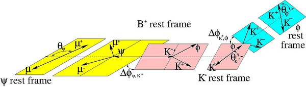
Definition of the $\theta_{ K ^* }$, $\theta_{ { J \mskip -3mu/\mskip -2mu\psi \mskip 2mu} }$, $\theta_{\phi}$, $\Delta{\phi}_{ K ^* , { J \mskip -3mu/\mskip -2mu\psi \mskip 2mu} }$ and $\Delta{\phi}_{ K ^* ,\phi }$ angles describing angular correlations in $B^+\rightarrow { J \mskip -3mu/\mskip -2mu\psi \mskip 2mu} K^{*+}$, $ { J \mskip -3mu/\mskip -2mu\psi \mskip 2mu} \rightarrow \mu^+\mu^-$, $K^{*+}\rightarrow \phi K^+$, $\phi\rightarrow K^+K^-$ decays ($ { J \mskip -3mu/\mskip -2mu\psi \mskip 2mu} $ is denoted as $\psi$ in the figure).

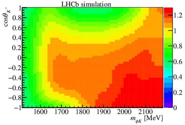
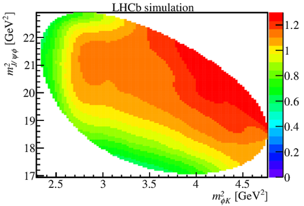
Parameterized efficiency $\epsilon_1(m_{\phi K},\cos\theta_{ K ^* })$ function (top) and its representation in the Dalitz plane $({m_{\phi K }^2},{m_{ { J \mskip -3mu/\mskip -2mu\psi \mskip 2mu} \phi }^2})$ (bottom). Function values corresponding to the color encoding are given on the right. The normalization arbitrarily corresponds to unity when averaged over the phase space.

Parameterized efficiency $\epsilon_2(\cos\theta_{\phi }|m_{\phi K})$, $\epsilon_3(\cos\theta_{ { J \mskip -3mu/\mskip -2mu\psi \mskip 2mu} }|m_{\phi K})$, $\epsilon_4(\Delta{\phi}_{ K ^* ,\phi }|m_{\phi K})$, $\epsilon_5(\Delta{\phi}_{ K ^* , { J \mskip -3mu/\mskip -2mu\psi \mskip 2mu} }|m_{\phi K})$ functions. Function values corresponding to the color encoding are given on the right. By construction each function integrates to unity at each $m_{\phi K}$ value. The structure in $\epsilon_2(\cos\theta_{\phi }|m_{\phi K})$ present between 1500 and $1600 \mathrm{ Me V} $ is an artifact of removing $B^+\rightarrow { J \mskip -3mu/\mskip -2mu\psi \mskip 2mu} K^+K^-K^+$ events in which both $K^+K^-$ combinations pass the $\phi$ mass selection window.

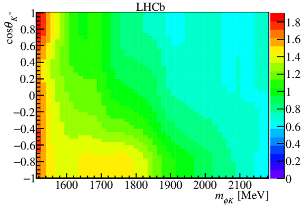
Parameterized background ${P_{\rm bkg}}_1(m_{\phi K},\cos\theta_{ K ^* })$ function (top) and its representation in the Dalitz plane $({m_{\phi K }^2},{m_{ { J \mskip -3mu/\mskip -2mu\psi \mskip 2mu} \phi }^2})$ (bottom). Function values corresponding to the color encoding are given on the right. The normalization arbitrarily corresponds to unity when averaged over the phase space.

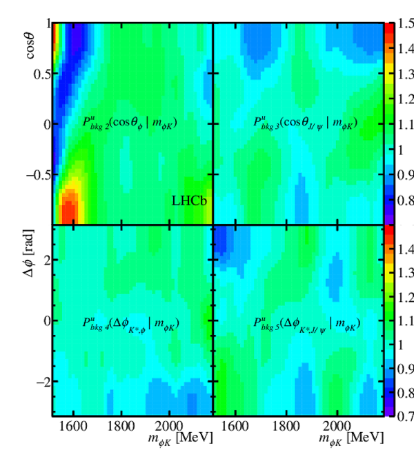
Parameterized background functions: $P^u_{\rm bkg 2}(\cos\theta_{\phi }|m_{\phi K })$, $P^u_{\rm bkg 3}(\cos\theta_{ { J \mskip -3mu/\mskip -2mu\psi \mskip 2mu} }|m_{\phi K })$, $P^u_{\rm bkg 4}(\Delta{\phi}_{ K ^* ,\phi }|m_{\phi K })$, $P^u_{\rm bkg 5}(\Delta{\phi}_{ K ^* , { J \mskip -3mu/\mskip -2mu\psi \mskip 2mu} }|m_{\phi K })$. Function values corresponding to the color encoding are given on the right. By construction each function integrates to unity at each $m_{\phi K}$ value.

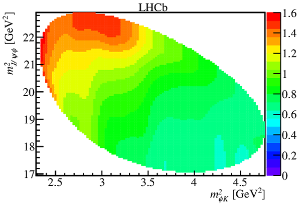
Background-subtracted and efficiency-corrected data yield in the Dalitz plane of $({m_{\phi K }^2},{m_{ { J \mskip -3mu/\mskip -2mu\psi \mskip 2mu} \phi }^2})$. Yield values corresponding to the color encoding are given on the right.

Background-subtracted and efficiency-corrected data yield in the Dalitz plane of $({m_{\phi K }^2},{m_{ { J \mskip -3mu/\mskip -2mu\psi \mskip 2mu} K }^2})$. Yield values corresponding to the color encoding are given on the right.

Background-subtracted and efficiency-corrected data yield in the Dalitz plane of $({m_{ { J \mskip -3mu/\mskip -2mu\psi \mskip 2mu} K }^2},{m_{ { J \mskip -3mu/\mskip -2mu\psi \mskip 2mu} \phi }^2})$. Yield values corresponding to the color encoding are given on the right.

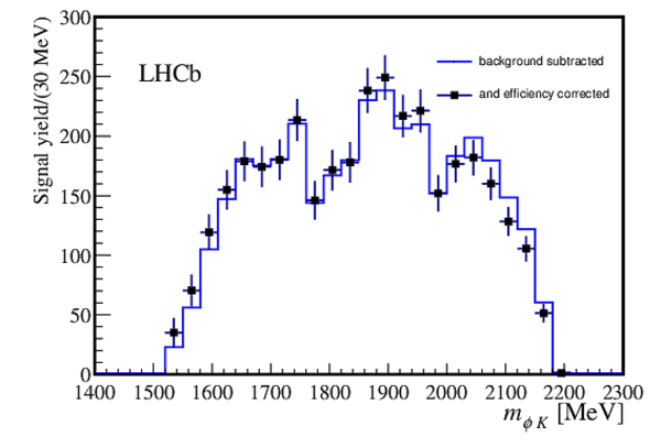
Background-subtracted (histogram) and efficiency-corrected (points) distribution of $m_{\phi K}$. See the text for the explanation of the efficiency normalization.

Background-subtracted (histogram) and efficiency-corrected (points) distribution of $m_{ { J \mskip -3mu/\mskip -2mu\psi \mskip 2mu} \phi}$. See the text for the explanation of the efficiency normalization.

Background-subtracted (histogram) and efficiency-corrected (points) distribution of $m_{ { J \mskip -3mu/\mskip -2mu\psi \mskip 2mu} K}$. See the text for the explanation of the efficiency normalization.

Kaon excitations predicted by Godfrey--Isgur [53] (horizontal black lines) labeled with their intrinsic quantum numbers: $n{}^{2S+1}L_J$ (see the text). Well established states are shown with narrower solid blue boxes extending to $\pm1\sigma$ in mass and labeled with their PDG names [37]. Unconfirmed states are shown with dashed green boxes. The long horizontal red lines indicate the $\phi K$ mass range probed in $B^+\rightarrow { J \mskip -3mu/\mskip -2mu\psi \mskip 2mu} \phi K^+$ decays.

Distribution of $m_{ { J \mskip -3mu/\mskip -2mu\psi \mskip 2mu} \phi}$ for the data and the fit results with a model containing only $K^{*+}\rightarrow \phi K^+$ contributions.

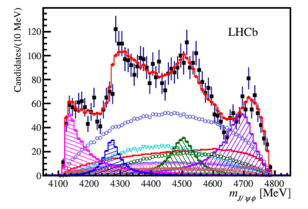
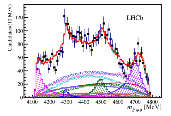
Distributions of (top left) $\phi K^+$, (top right) $ { J \mskip -3mu/\mskip -2mu\psi \mskip 2mu} K^+$ and (bottom) $ { J \mskip -3mu/\mskip -2mu\psi \mskip 2mu} \phi$ invariant masses for the $B^+\rightarrow { J \mskip -3mu/\mskip -2mu\psi \mskip 2mu} \phi K^+$ data (black data points) compared with the results of the default amplitude fit containing $K^{*+}\rightarrow \phi K^+$ and $X\rightarrow { J \mskip -3mu/\mskip -2mu\psi \mskip 2mu} \phi$ contributions. The total fit is given by the red points with error bars. Individual fit components are also shown. Displays of $m_{ { J \mskip -3mu/\mskip -2mu\psi \mskip 2mu} \phi}$ and of $m_{ { J \mskip -3mu/\mskip -2mu\psi \mskip 2mu} K}$ masses in slices of $m_{\phi K}$ are shown in Fig. 20.

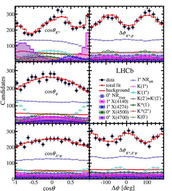
Distributions of the fitted decay angles from the $K^{*+}$ decay chain together with the display of the default fit model described in the text.

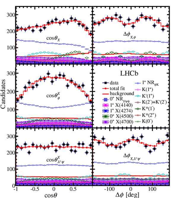
Distributions of the fitted decay angles from the $X$ decay chain together with the display of the default fit model described in the text.

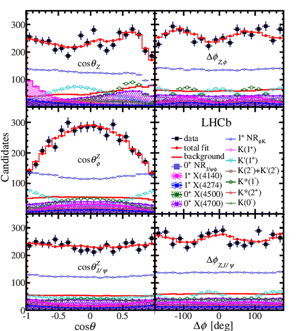
Distributions of the fitted decay angles from the $Z$ decay chain together with the display of the default fit model described in the text.

Distribution of (left) $m_{ { J \mskip -3mu/\mskip -2mu\psi \mskip 2mu} \phi}$ and (right) $m_{ { J \mskip -3mu/\mskip -2mu\psi \mskip 2mu} K}$ in three slices of $m_{\phi K }$: $<1750 \mathrm{ Me V} $, $1750-1950 \mathrm{ Me V} $, and $>1950 \mathrm{ Me V} $ from the top to the bottom, together with the projections of the default amplitude model. See the legend in Fig. 16 for a description of the components.

Mass of $B^+\rightarrow { J \mskip -3mu/\mskip -2mu\psi \mskip 2mu} \phi K^+$ candidates in the data with the $ p_{\mathrm{ T}} (K)>250 \mathrm{ Me V} $ (default) and $ p_{\mathrm{ T}} (K)>500 \mathrm{ Me V} $ selection requirements.

Distributions of (top) $\phi K^+$, (middle) $ { J \mskip -3mu/\mskip -2mu\psi \mskip 2mu} K^+$ and (bottom) $ { J \mskip -3mu/\mskip -2mu\psi \mskip 2mu} \phi$ invariant masses for the $B^+\rightarrow { J \mskip -3mu/\mskip -2mu\psi \mskip 2mu} \phi K^+$ data after changing the $ p_{\mathrm{ T}} (K)>0.25 \mathrm{ Ge V} $ requirement to $ p_{\mathrm{ T}} (K)>0.5 \mathrm{ Ge V} $, together with the fit projections. Compare to Fig. 16.

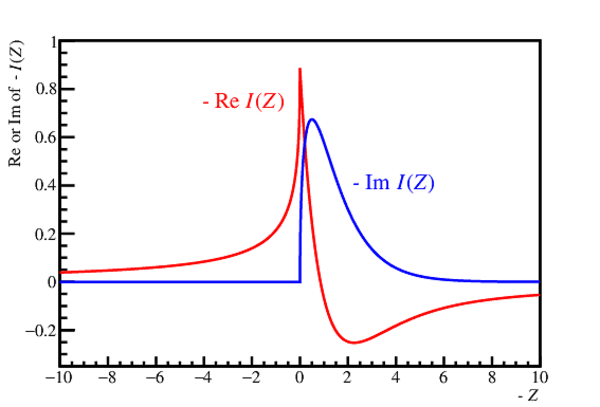
Dependence of the real and imaginary parts of the cusp amplitude on the mass in Swanson's model [61]. See the text for a more precise explanation.

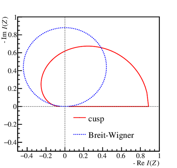
The Argand diagram of the the cusp amplitude in Swanson's model [61]. Motion with the mass is counter-clockwise. The peak amplitude is reached at threshold when the real part is maximal and the imaginary part is zero. The Breit--Wigner amplitude gives circular phase motion, also with counter-clockwise mass evolution, with maximum magnitude when zero is crossed on the real axis.

Distributions of (top left) $\phi K^+$, (top right) $ { J \mskip -3mu/\mskip -2mu\psi \mskip 2mu} K^+$ and (bottom) $ { J \mskip -3mu/\mskip -2mu\psi \mskip 2mu} \phi$ invariant masses for the $B^+\rightarrow { J \mskip -3mu/\mskip -2mu\psi \mskip 2mu} \phi K^+$ data (black data points) compared with the results of the amplitude fit containing $K^{*+}\rightarrow \phi K^+$ and $X\rightarrow { J \mskip -3mu/\mskip -2mu\psi \mskip 2mu} \phi$ contributions in which $X(4140)$ is represented as a $J^{PC}=1^{++}$ $D_s^+D_s^{*-}$ cusp. The total fit is given by the red points with error bars. Individual fit components are also shown.

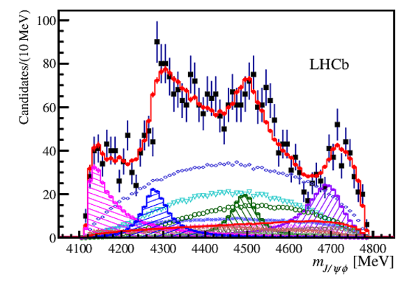
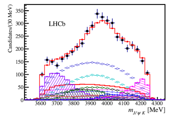
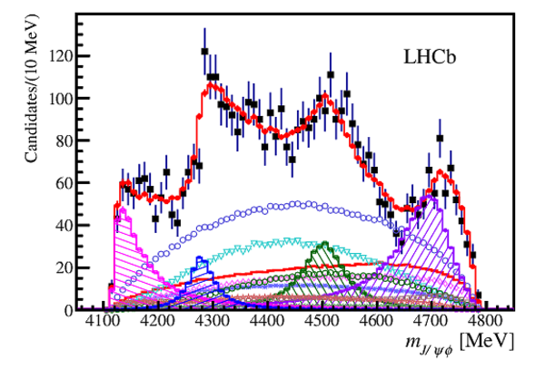
Distributions of $ { J \mskip -3mu/\mskip -2mu\psi \mskip 2mu} \phi$ invariant mass for the $B^+\rightarrow { J \mskip -3mu/\mskip -2mu\psi \mskip 2mu} \phi K^+$ data (black data points) compared with the results of the amplitude fit containing $K^{*+}\rightarrow \phi K^+$ and $X\rightarrow { J \mskip -3mu/\mskip -2mu\psi \mskip 2mu} \phi$ contributions in which $X(4140)$ and $X(4274)$ are represented as $J^{PC}=1^{++}$ $D_s^\pm D_s^{*\mp}$ and $0^{-+}$ $D_s^{\pm}D_{s0}^{*}(2317)^{\mp}$ cusps, respectively. The total fit is given by the red points with error bars. Individual fit components are also shown.

Animated gif made out of all figures.

Previous results related to the $X(4140)\rightarrow { J \mskip -3mu/\mskip -2mu\psi \mskip 2mu} \phi$ mass peak, first observed in $B^+\rightarrow { J \mskip -3mu/\mskip -2mu\psi \mskip 2mu} \phi K^+$ decays. The first (second) significance quoted for Ref. [27] is for the prompt (non-prompt) production components. The statistical and systematic errors are added in quadrature and then used in the weights to calculate the averages, excluding unpublished results (shown in italics). The last column gives a fraction of the total $B^+\rightarrow { J \mskip -3mu/\mskip -2mu\psi \mskip 2mu} \phi K^+$ rate attributed to the $X(4140)$ structure.

Previous results related to $ { J \mskip -3mu/\mskip -2mu\psi \mskip 2mu} \phi$ mass structures heavier than the $X(4140)$ peak. The unpublished results are shown in italics.

Results for significances, masses, widths and fit fractions of the components included in the default amplitude model. The first (second) errors are statistical (systematic). Errors on $f_L$ and $f_\perp$ are statistical only. Possible interpretations in terms of kaon excitation levels are given, with notation $n{}^{2S+1}L_J$, together with the masses predicted in the Godfrey-Isgur model [53]. Comparisons with the previously experimentally observed kaon excitations [37] and $X\rightarrow { J \mskip -3mu/\mskip -2mu\psi \mskip 2mu} \phi$ structures are also given.

Summary of the systematic uncertainties on the parameters of the $K^{*+}\rightarrow \phi K^+$ states with $J^P=2^-$ and $1^+$. The kaon $ p_{\mathrm{ T}} $ cross-check results are given at the bottom. All numbers for masses and widths are in $\mathrm{ Me V}$ and fit fractions in %.

Summary of the systematic uncertainties on the parameters of the $K^{*+}\rightarrow \phi K^+$ states with $J^P=0^-$, $1^-$ and $2^+$. The kaon $ p_{\mathrm{ T}} $ cross-check results are given at the bottom. All numbers for masses and widths are in $\mathrm{ Me V}$ and fit fractions in %.

Summary of the systematic uncertainties on the parameters of the $X\rightarrow { J \mskip -3mu/\mskip -2mu\psi \mskip 2mu} \phi$ states. The kaon $ p_{\mathrm{ T}} $ cross-check results are given at the bottom. All numbers for masses and widths are in $\mathrm{ Me V}$ and fit fractions in %.

Statistical significance of $J^{PC}$ preference for the $X$ states in the default model. The lowest significance value for each state is highlighted.

Significance, in standard deviations, of $J^{PC}$ preference for the $X$ states for dominant systematic variations of the fit model. The label "$L+n$" specifies which $L$ value in Eq. (9) is increased relative to its minimal value and by how much ($n$). The lowest significance value for each state is highlighted.