

Compact Muon Solenoid
LHC, CERN
| CMS-EXO-14-015 ; CERN-PH-EP-2015-281 | ||
| Search for excited leptons in proton-proton collisions at $ \sqrt{s} = $ 8 TeV | ||
| CMS Collaboration | ||
| 4 November 2015 | ||
| J. High Energy Phys. 03 (2016) 125 | ||
| Abstract: A search for compositeness of electrons and muons is presented using a data sample of proton-proton collisions at a center-of-mass energy of $ \sqrt{s} = $ 8 TeV collected with the CMS detector at the LHC and corresponding to an integrated luminosity of 19.7 fb$^{-1}$. Excited leptons ($\ell^*$) produced via contact interactions in conjunction with a standard model lepton are considered, and a search is made for their gauge decay modes. The decays considered are $\ell^* \to \ell \gamma$ and $\ell^* \to \ell \mathrm{ Z }$, which give final states of two leptons and a photon or, depending on the Z-boson decay mode, four leptons or two leptons and two jets. The number of events observed in data is consistent with the standard model prediction. Exclusion limits are set on the excited lepton mass, and the compositeness scale $\Lambda$. For the case $M_{\ell^*} = \Lambda$ the existence of excited electrons (muons) is excluded up to masses of 2.45 (2.47) TeV at 95% confidence level. Neutral current decays of excited leptons are considered for the first time, and limits are extended to include the possibility that the weight factors $f$ and $f^{\prime}$, which determine the couplings between standard model leptons and excited leptons via gauge mediated interactions, have opposite sign. | ||
| Links: e-print arXiv:1511.01407 [hep-ex] (PDF) ; CDS record ; inSPIRE record ; CADI line (restricted) ; | ||
| Figures | |
png pdf |
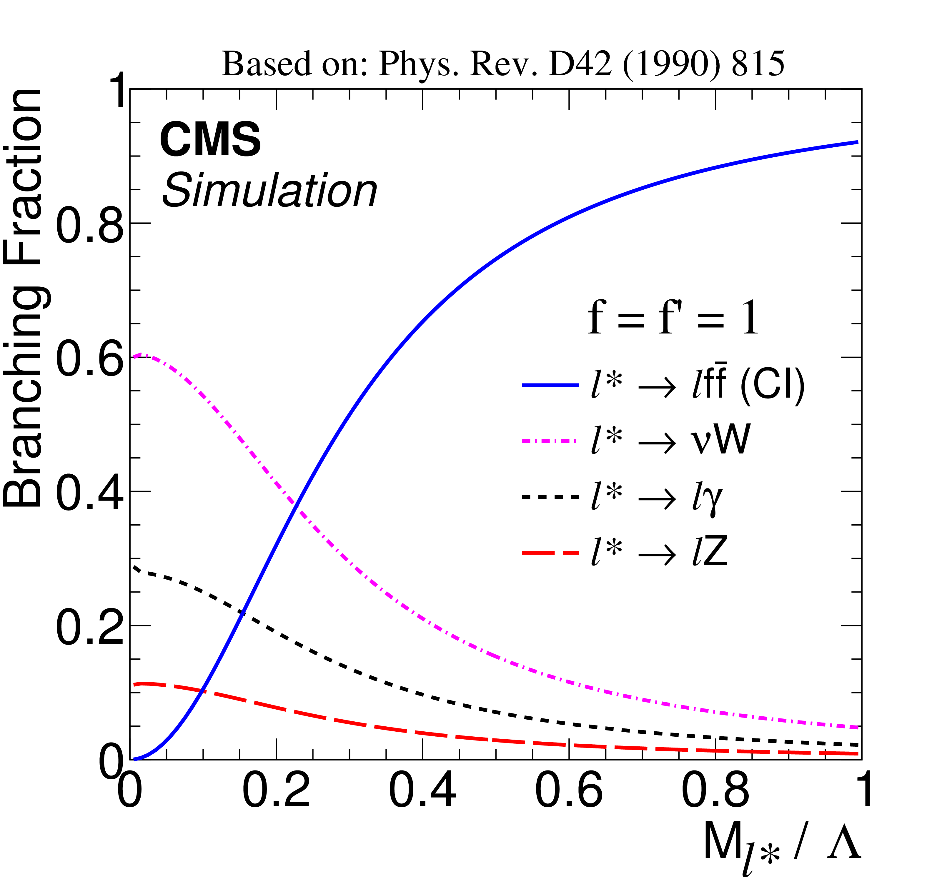
Figure 1-a:
Branching fractions for the decay of excited leptons, as a function of the ratio $M_{\ell ^{*}} / \Lambda $ of their mass to their compositeness scale, for the coupling weight factors $f = f^{\prime } =$ 1 (a) and $f = -f^{\prime } =$ 1 (b). The process $ {\ell ^*} \to \ell \mathrm{ f \bar{f} }$ indicates the decay via CI, while the other processes are gauge mediated decays. |
png pdf |
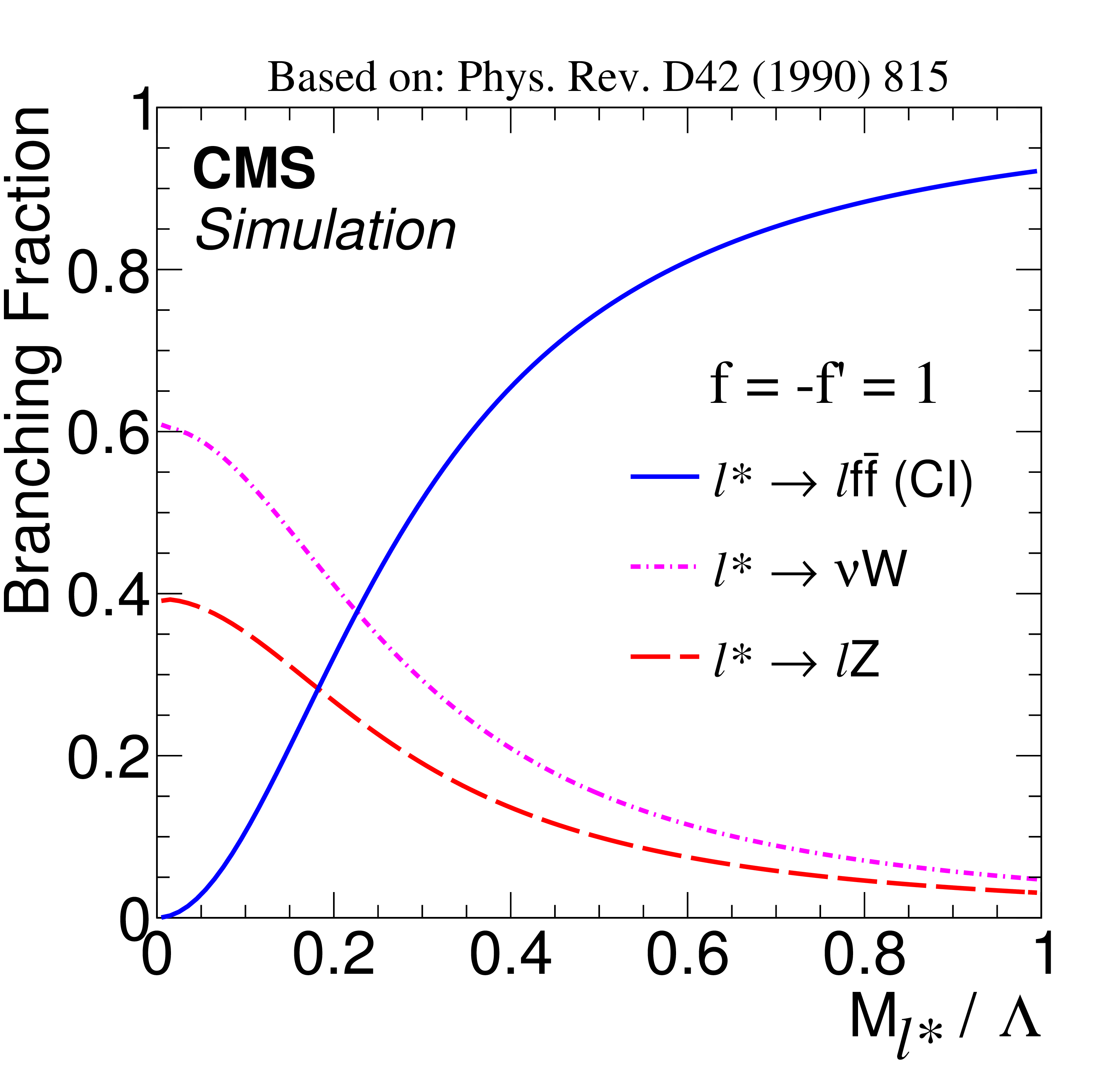
Figure 1-b:
Branching fractions for the decay of excited leptons, as a function of the ratio $M_{\ell ^{*}} / \Lambda $ of their mass to their compositeness scale, for the coupling weight factors $f = f^{\prime } =$ 1 (a) and $f = -f^{\prime } =$ 1 (b). The process $ {\ell ^*} \to \ell \mathrm{ f \bar{f} }$ indicates the decay via CI, while the other processes are gauge mediated decays. |
png pdf |
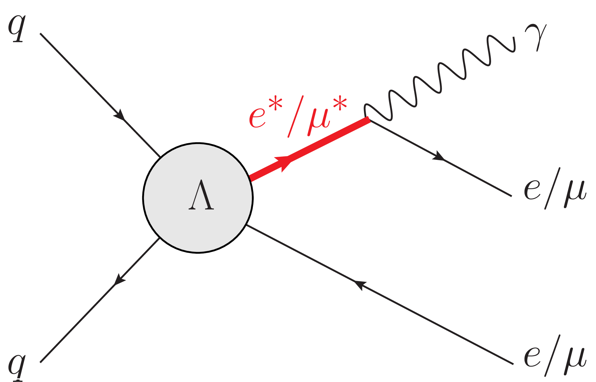
Figure 2-a:
Illustrative diagrams for ${\ell \ell ^* \to \ell \ell \gamma }$, where $\ell = \mathrm{ e } $, $\mu $. Decays of the Z boson to a pair of electrons, muons or jets are considered. |
png pdf |
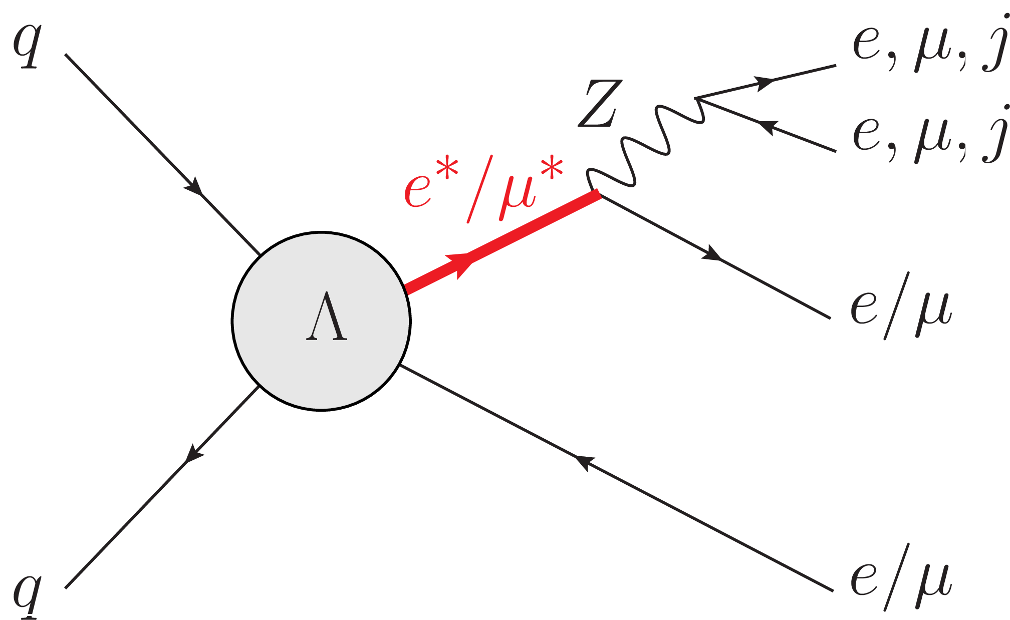
Figure 2-b:
Illustrative diagrams for ${\ell \ell \mathrm{ Z } }$, where $\ell = \mathrm{ e } $, $\mu $. Decays of the Z boson to a pair of electrons, muons or jets are considered. |
png pdf |
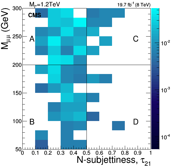
Figure 3-a:
Invariant mass of the pair of isolated muons vs. the N-subjettiness ratio, $\tau _{21}$, of the selected fat jet, for events passing the selection criteria given in Section 4.3, but with the cuts on $M_{\ell \ell }$ and $\tau _{21}$ relaxed for signal with $M_{\ell ^*}=$ 1.2 TeV (a), Drell-Yan+jets (b), $ {\mathrm{ t \bar{t} } } $+jets (c) and diboson events (d). The right hand scale gives to the number of events corresponding to the given integrated luminosity and the respective cross sections of the processes. |
png pdf |
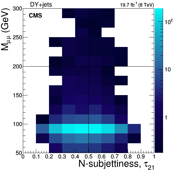
Figure 3-b:
Invariant mass of the pair of isolated muons vs. the N-subjettiness ratio, $\tau _{21}$, of the selected fat jet, for events passing the selection criteria given in Section 4.3, but with the cuts on $M_{\ell \ell }$ and $\tau _{21}$ relaxed for signal with $M_{\ell ^*}=$ 1.2 TeV (a), Drell-Yan+jets (b), $ {\mathrm{ t \bar{t} } } $+jets (c) and diboson events (d). The right hand scale gives to the number of events corresponding to the given integrated luminosity and the respective cross sections of the processes. |
png pdf |
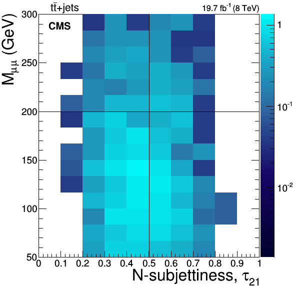
Figure 3-c:
Invariant mass of the pair of isolated muons vs. the N-subjettiness ratio, $\tau _{21}$, of the selected fat jet, for events passing the selection criteria given in Section 4.3, but with the cuts on $M_{\ell \ell }$ and $\tau _{21}$ relaxed for signal with $M_{\ell ^*}=$ 1.2 TeV (a), Drell-Yan+jets (b), $ {\mathrm{ t \bar{t} } } $+jets (c) and diboson events (d). The right hand scale gives to the number of events corresponding to the given integrated luminosity and the respective cross sections of the processes. |
png pdf |
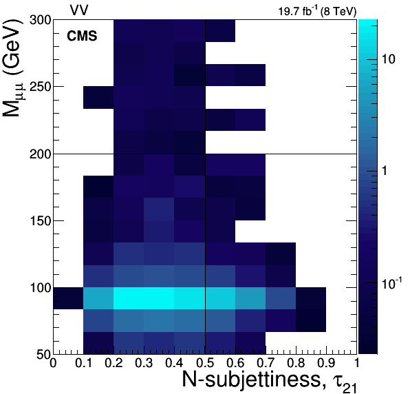
Figure 3-d:
Invariant mass of the pair of isolated muons vs. the N-subjettiness ratio, $\tau _{21}$, of the selected fat jet, for events passing the selection criteria given in Section 4.3, but with the cuts on $M_{\ell \ell }$ and $\tau _{21}$ relaxed for signal with $M_{\ell ^*}=$ 1.2 TeV (a), Drell-Yan+jets (b), $ {\mathrm{ t \bar{t} } } $+jets (c) and diboson events (d). The right hand scale gives to the number of events corresponding to the given integrated luminosity and the respective cross sections of the processes. |
png pdf |
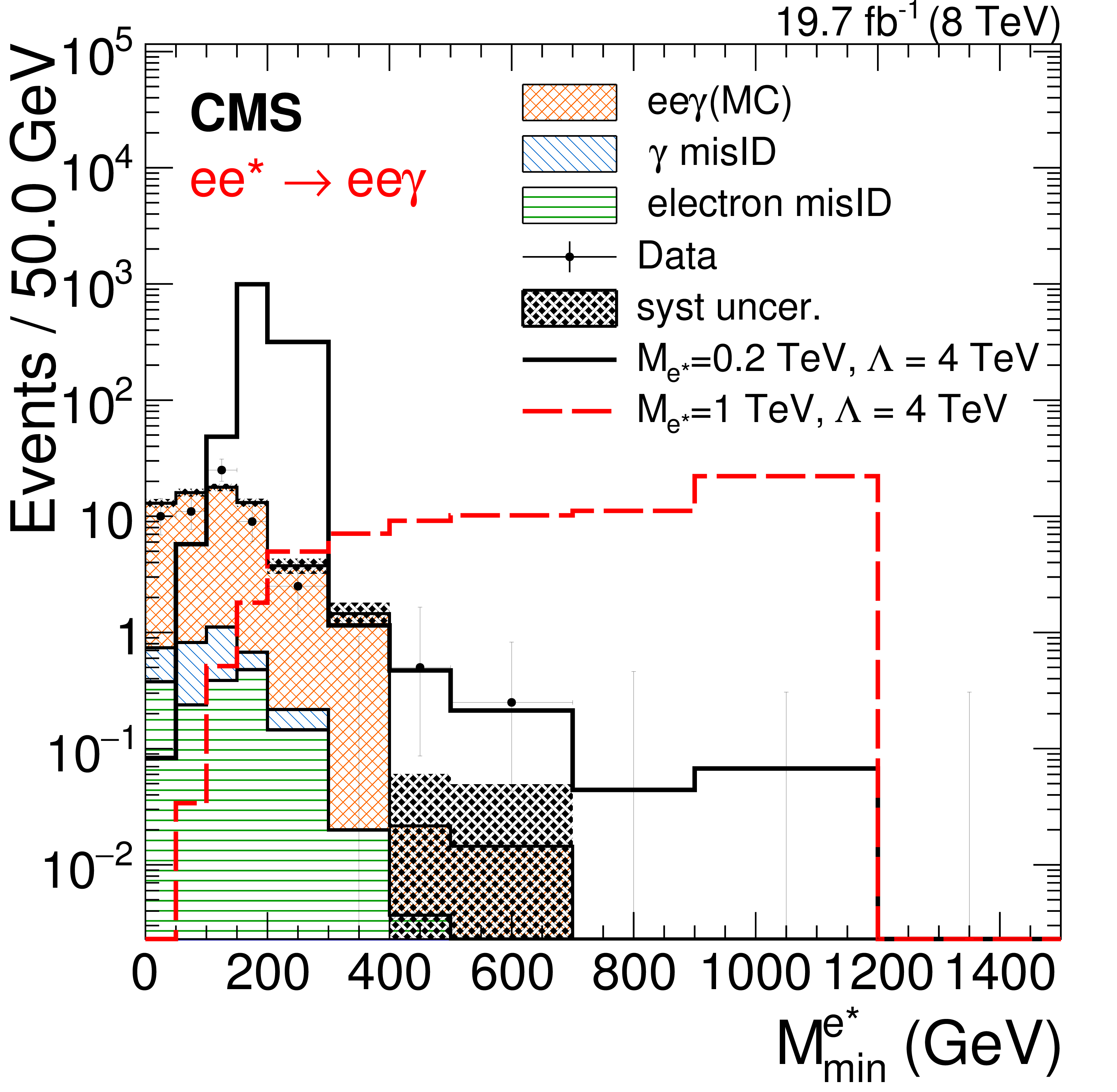
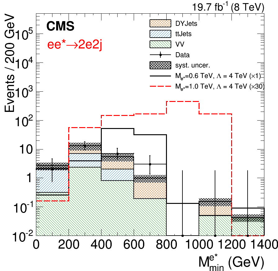
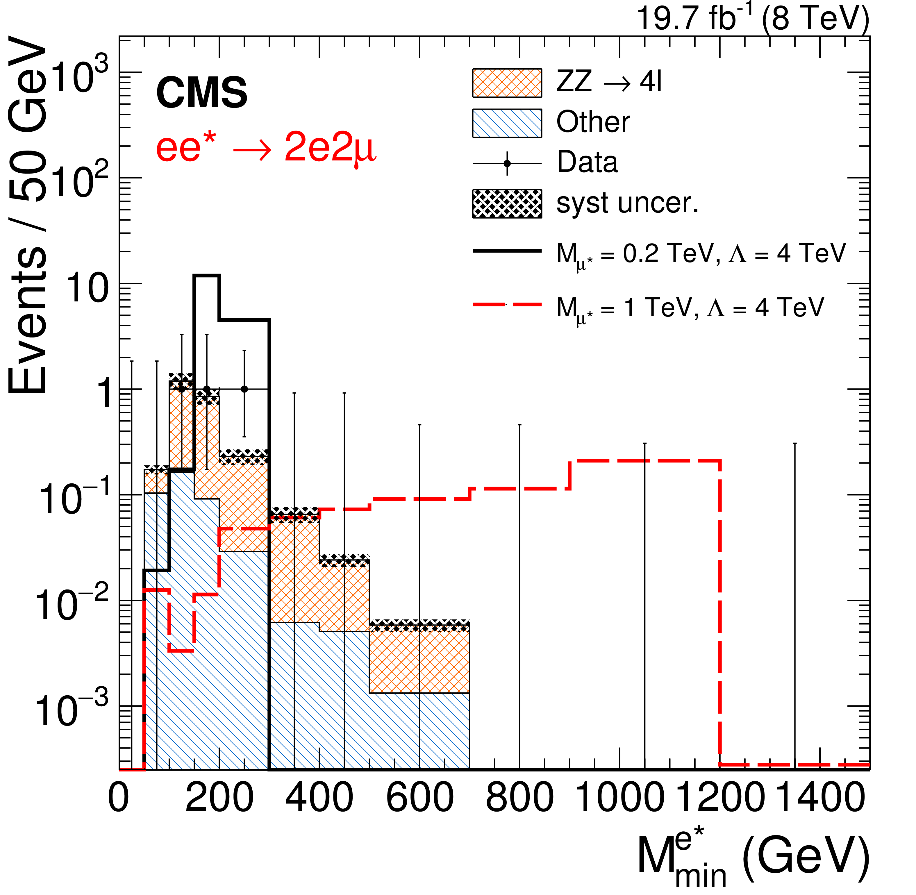
Figure 4-a:
Reconstructed minimum invariant mass from the vector boson ($\gamma $, $\mathrm{ Z } $) plus one electron for the four excited electron channels. a: $\mathrm{ e } \mathrm{ e } \gamma $, b: $2\mathrm{ e } 2 {\mathrm {j}} $, c: $4\mathrm{ e } $, d: $2\mathrm{ e } 2\mu $. Two signal distributions are shown for ${M_{\ell ^*}} = $ 0.2 and 1 TeV, except the $2\mathrm{ e } 2 {\mathrm {j}} $ channel where the trigger threshold only allows searches for $ {M_{\ell ^*}} > $ 0.5 TeV. The asymmetric error bars indicate the central confidence intervals for Poisson-distributed data and are obtained from the Neyman construction as described in Ref. [60]. |
png pdf |
Figure 4-b:
Reconstructed minimum invariant mass from the vector boson ($\gamma $, $\mathrm{ Z } $) plus one electron for the four excited electron channels. a: $\mathrm{ e } \mathrm{ e } \gamma $, b: $2\mathrm{ e } 2 {\mathrm {j}} $, c: $4\mathrm{ e } $, d: $2\mathrm{ e } 2\mu $. Two signal distributions are shown for ${M_{\ell ^*}} = $ 0.2 and 1 TeV, except the $2\mathrm{ e } 2 {\mathrm {j}} $ channel where the trigger threshold only allows searches for $ {M_{\ell ^*}} > $ 0.5 TeV. The asymmetric error bars indicate the central confidence intervals for Poisson-distributed data and are obtained from the Neyman construction as described in Ref. [60]. |

png pdf |
Figure 4-c:
Reconstructed minimum invariant mass from the vector boson ($\gamma $, $\mathrm{ Z } $) plus one electron for the four excited electron channels. a: $\mathrm{ e } \mathrm{ e } \gamma $, b: $2\mathrm{ e } 2 {\mathrm {j}} $, c: $4\mathrm{ e } $, d: $2\mathrm{ e } 2\mu $. Two signal distributions are shown for ${M_{\ell ^*}} = $ 0.2 and 1 TeV, except the $2\mathrm{ e } 2 {\mathrm {j}} $ channel where the trigger threshold only allows searches for $ {M_{\ell ^*}} > $ 0.5 TeV. The asymmetric error bars indicate the central confidence intervals for Poisson-distributed data and are obtained from the Neyman construction as described in Ref. [60]. |
png pdf |
Figure 4-d:
Reconstructed minimum invariant mass from the vector boson ($\gamma $, $\mathrm{ Z } $) plus one electron for the four excited electron channels. a: $\mathrm{ e } \mathrm{ e } \gamma $, b: $2\mathrm{ e } 2 {\mathrm {j}} $, c: $4\mathrm{ e } $, d: $2\mathrm{ e } 2\mu $. Two signal distributions are shown for ${M_{\ell ^*}} = $ 0.2 and 1 TeV, except the $2\mathrm{ e } 2 {\mathrm {j}} $ channel where the trigger threshold only allows searches for $ {M_{\ell ^*}} > $ 0.5 TeV. The asymmetric error bars indicate the central confidence intervals for Poisson-distributed data and are obtained from the Neyman construction as described in Ref. [60]. |
png pdf |
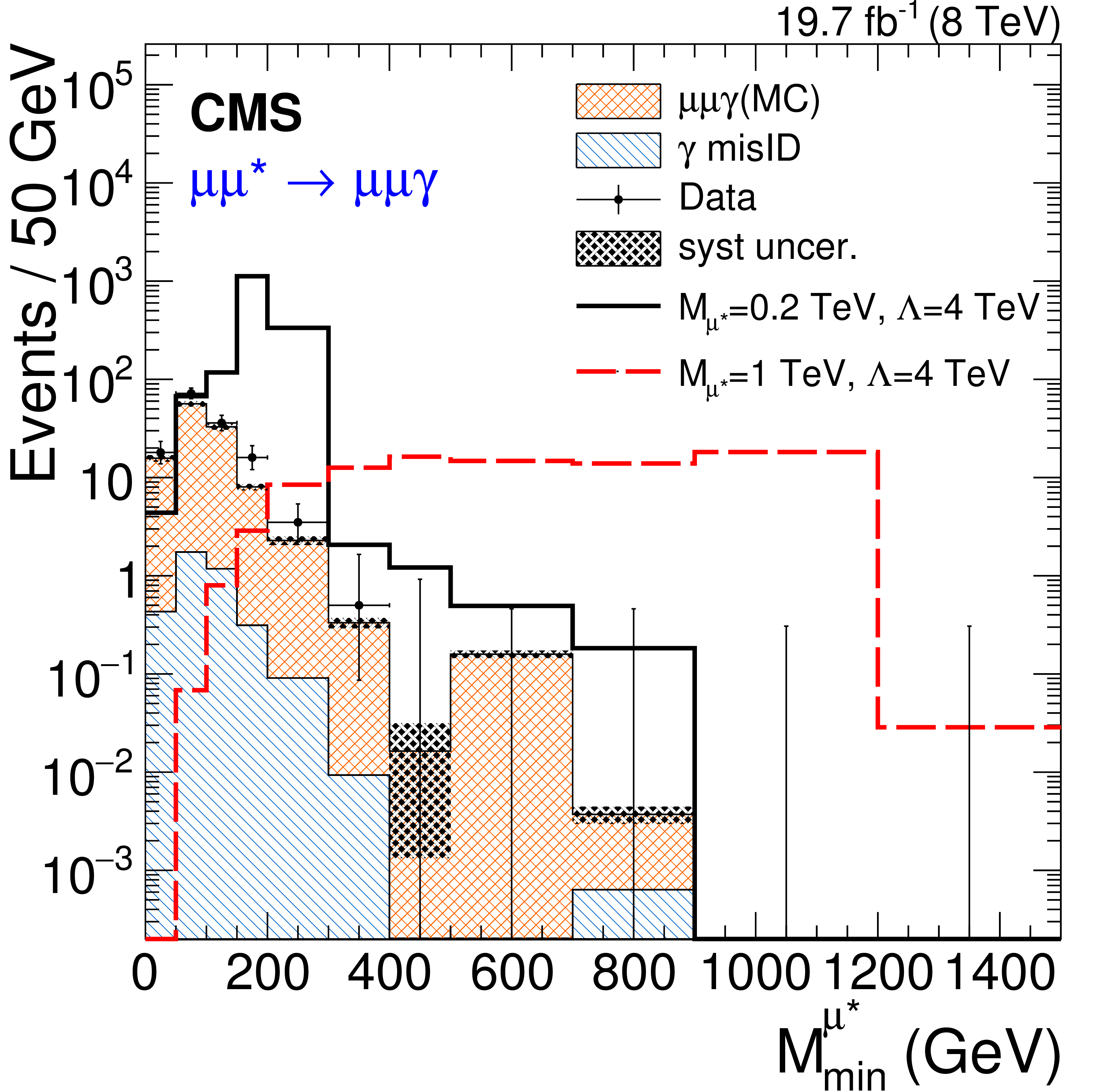
Figure 5-a:
Reconstructed minimum invariant mass from the vector boson ($\gamma $, $\mathrm{ Z } $) plus one muon for the four excited muon channels. a: $\mu \mu \gamma $, b: $2\mu 2 {\mathrm {j}} $, c: $4\mu $, d: $2\mu 2\mathrm{ e } $. Two signal distributions are shown for ${M_{\ell ^*}} =$ 0.2 and 1 TeV, except the $2\mu 2 {\mathrm {j}} $ channel where the trigger threshold only allows searches for $ {M_{\ell ^*}} >$ 0.5 TeV. The asymmetric error bars indicate the central confidence intervals for Poisson-distributed data and are obtained from the Neyman construction as described in Ref. [60]. |
png pdf |
Figure 5-b:
Reconstructed minimum invariant mass from the vector boson ($\gamma $, $\mathrm{ Z } $) plus one muon for the four excited muon channels. a: $\mu \mu \gamma $, b: $2\mu 2 {\mathrm {j}} $, c: $4\mu $, d: $2\mu 2\mathrm{ e } $. Two signal distributions are shown for ${M_{\ell ^*}} =$ 0.2 and 1 TeV, except the $2\mu 2 {\mathrm {j}} $ channel where the trigger threshold only allows searches for $ {M_{\ell ^*}} >$ 0.5 TeV. The asymmetric error bars indicate the central confidence intervals for Poisson-distributed data and are obtained from the Neyman construction as described in Ref. [60]. |
png pdf |
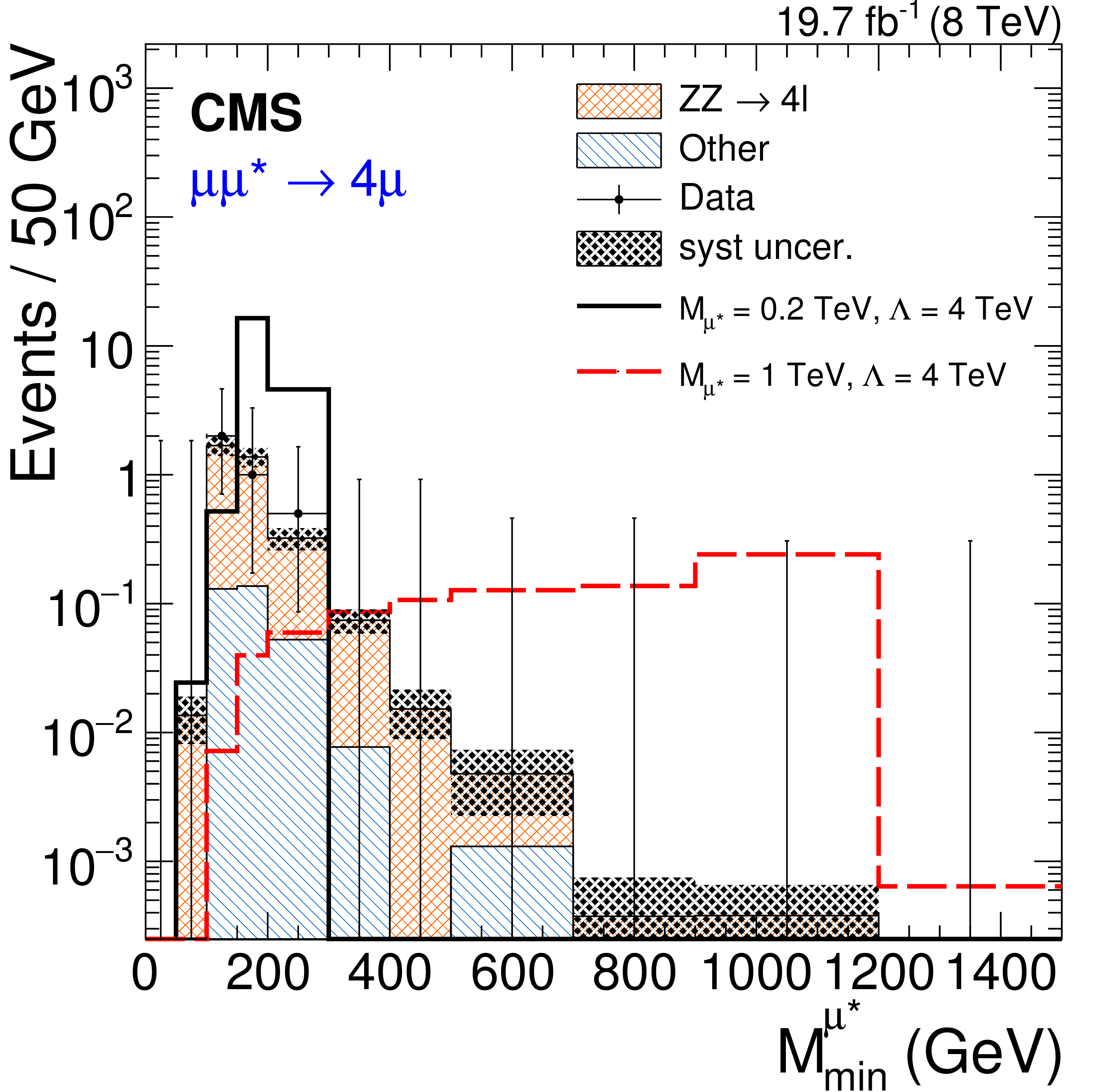
Figure 5-c:
Reconstructed minimum invariant mass from the vector boson ($\gamma $, $\mathrm{ Z } $) plus one muon for the four excited muon channels. a: $\mu \mu \gamma $, b: $2\mu 2 {\mathrm {j}} $, c: $4\mu $, d: $2\mu 2\mathrm{ e } $. Two signal distributions are shown for ${M_{\ell ^*}} =$ 0.2 and 1 TeV, except the $2\mu 2 {\mathrm {j}} $ channel where the trigger threshold only allows searches for $ {M_{\ell ^*}} >$ 0.5 TeV. The asymmetric error bars indicate the central confidence intervals for Poisson-distributed data and are obtained from the Neyman construction as described in Ref. [60]. |

png pdf |
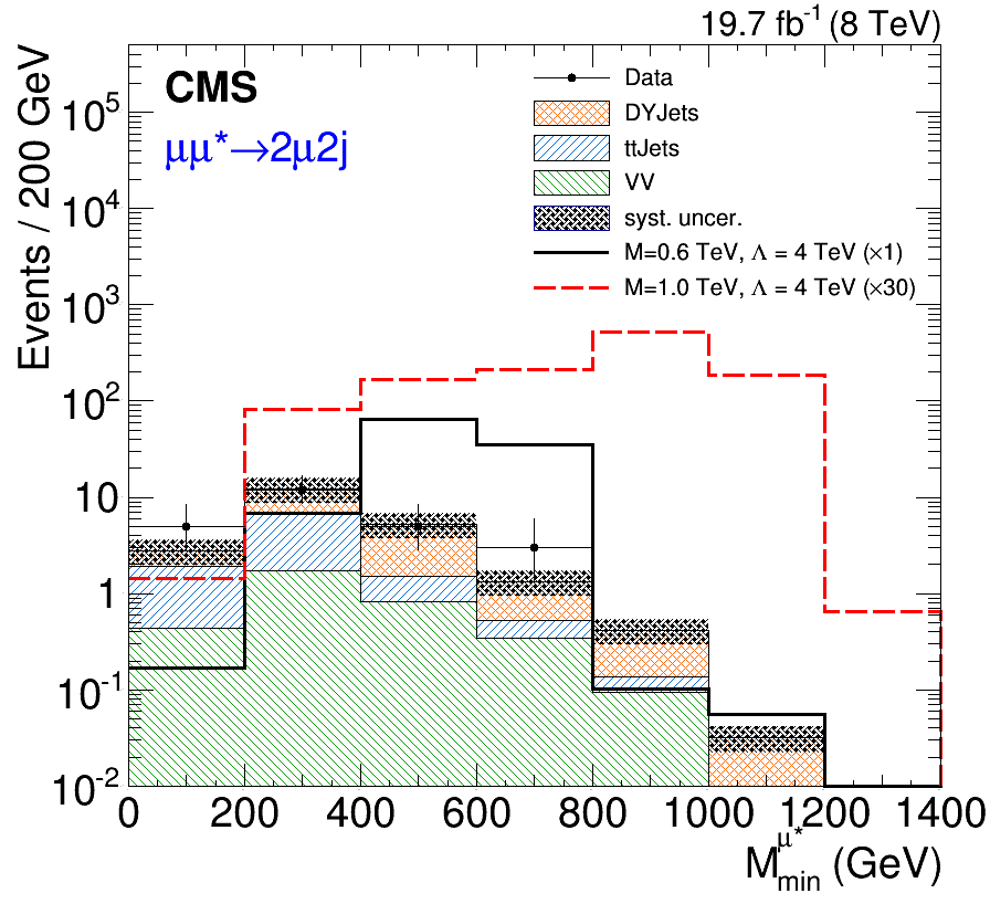
Figure 5-d:
Reconstructed minimum invariant mass from the vector boson ($\gamma $, $\mathrm{ Z } $) plus one muon for the four excited muon channels. a: $\mu \mu \gamma $, b: $2\mu 2 {\mathrm {j}} $, c: $4\mu $, d: $2\mu 2\mathrm{ e } $. Two signal distributions are shown for ${M_{\ell ^*}} =$ 0.2 and 1 TeV, except the $2\mu 2 {\mathrm {j}} $ channel where the trigger threshold only allows searches for $ {M_{\ell ^*}} >$ 0.5 TeV. The asymmetric error bars indicate the central confidence intervals for Poisson-distributed data and are obtained from the Neyman construction as described in Ref. [60]. |

png pdf |
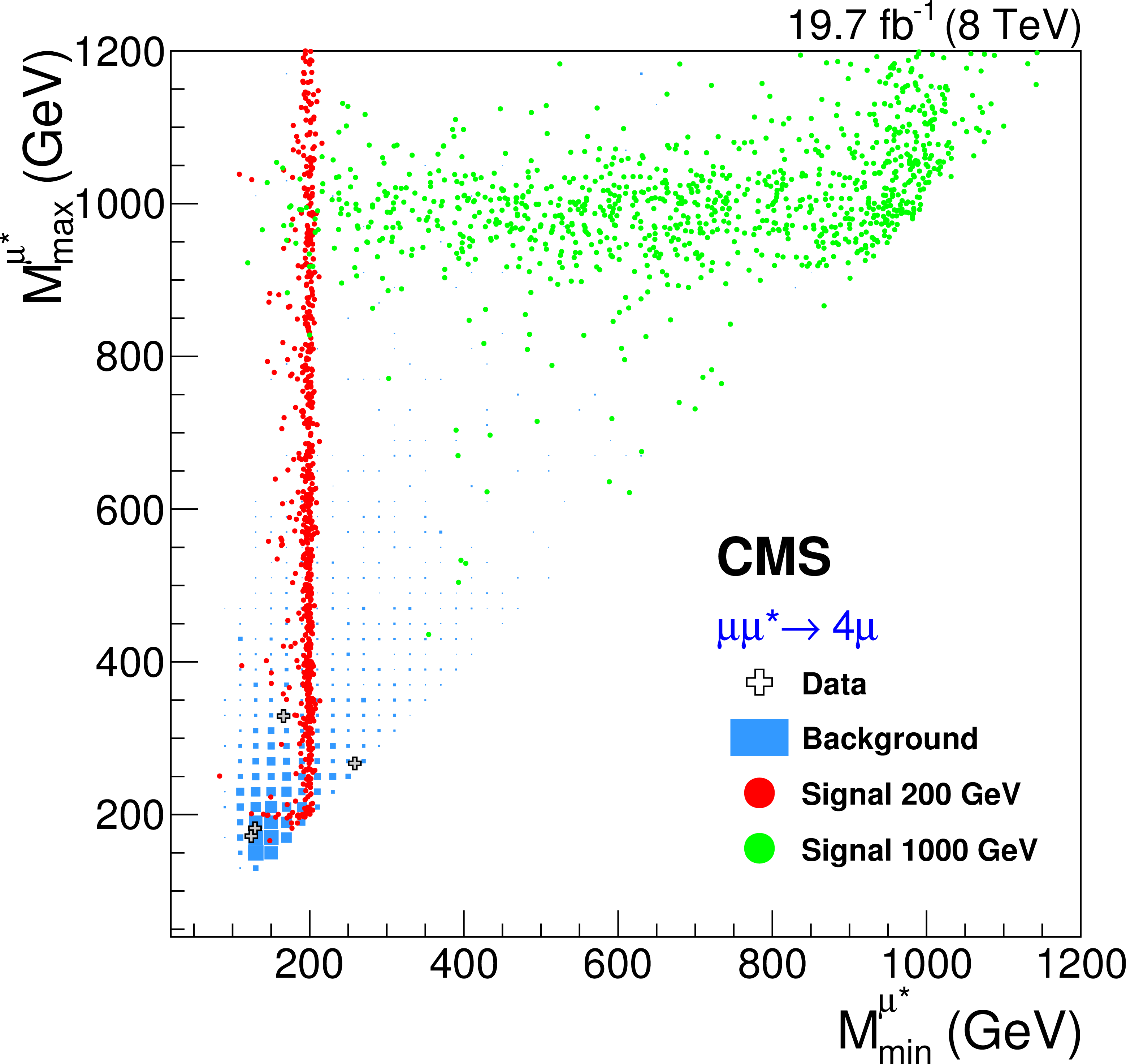
Figure 6-a:
Illustrative two dimensional minimal-versus-maximal invariant-mass distribution for the ${ \mathrm{ e } \mathrm{ e } ^* \to \mathrm{ e } \mathrm{ e } \gamma }$ (a) and the $4\mu $ channel (b). It can be seen that the resolution worsens with increasing signal mass and that the channels have different resolutions. The left plot clearly shows the effect of the additional Z-veto that is applied in this channel. Background contributions are normalized to the given integrated luminosity, while the normalization of the signal was chosen to enhance visibility. |
png pdf |
Figure 6-b:
Illustrative two dimensional minimal-versus-maximal invariant-mass distribution for the ${ \mathrm{ e } \mathrm{ e } ^* \to \mathrm{ e } \mathrm{ e } \gamma }$ (a) and the $4\mu $ channel (b). It can be seen that the resolution worsens with increasing signal mass and that the channels have different resolutions. The left plot clearly shows the effect of the additional Z-veto that is applied in this channel. Background contributions are normalized to the given integrated luminosity, while the normalization of the signal was chosen to enhance visibility. |
png pdf |
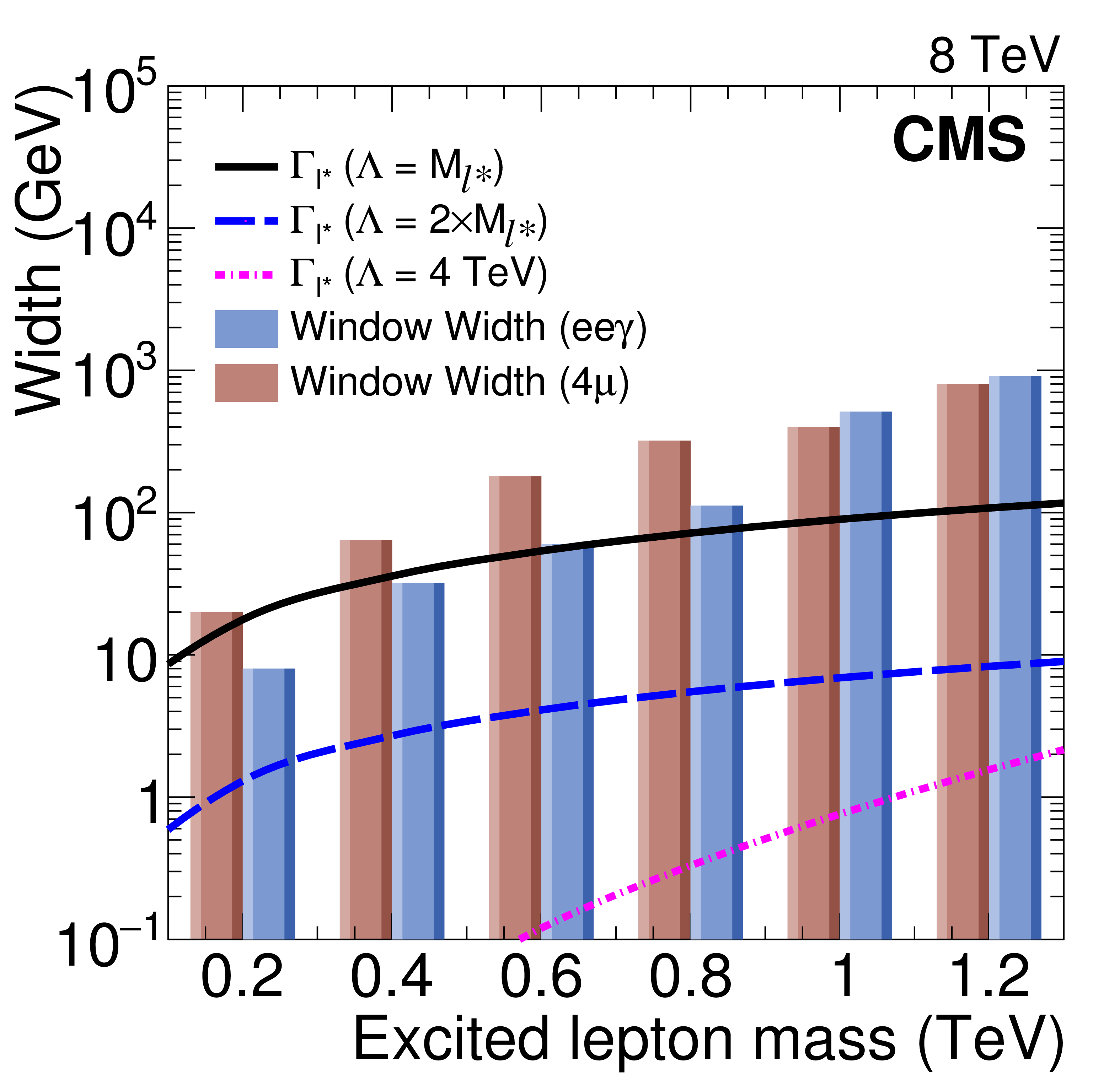
Figure 7:
Width of the widest search window ($4\mu $ channel) and of a narrow one ($\mathrm{ e } \mathrm{ e } \gamma $) compared with the intrinsic decay width of the excited lepton, as a function of the ${\ell ^*}$ mass and for different values of $\Lambda $. The latter shows the width of the excited leptons as defined in Ref. [7], including GM and CI decays, for the case $f = -f^{\prime } = $ 1. |

png pdf |
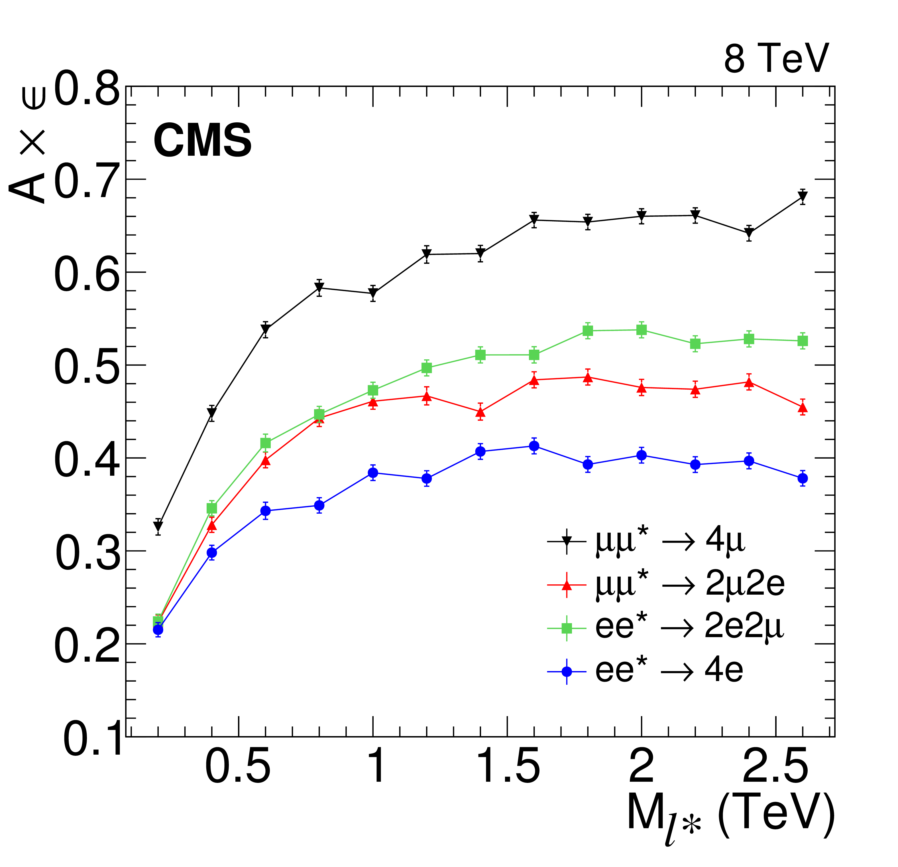
Figure 8-a:
The product of acceptance and efficiency after L-shape selection. In the left panel, the efficiencies for the ${\ell \ell ^* \to \ell \ell \gamma }$ and $2\ell 2 {\mathrm {j}} $ channels are shown while the right panel gives the efficiencies of the four-lepton channels. For the $2\ell 2 {\mathrm {j}} $ and $4\ell $ channels, the values do not include the branching fractions for the specific Z boson decay channel. |
png pdf |
Figure 8-b:
The product of acceptance and efficiency after L-shape selection. In the left panel, the efficiencies for the ${\ell \ell ^* \to \ell \ell \gamma }$ and $2\ell 2 {\mathrm {j}} $ channels are shown while the right panel gives the efficiencies of the four-lepton channels. For the $2\ell 2 {\mathrm {j}} $ and $4\ell $ channels, the values do not include the branching fractions for the specific Z boson decay channel. |
png pdf |
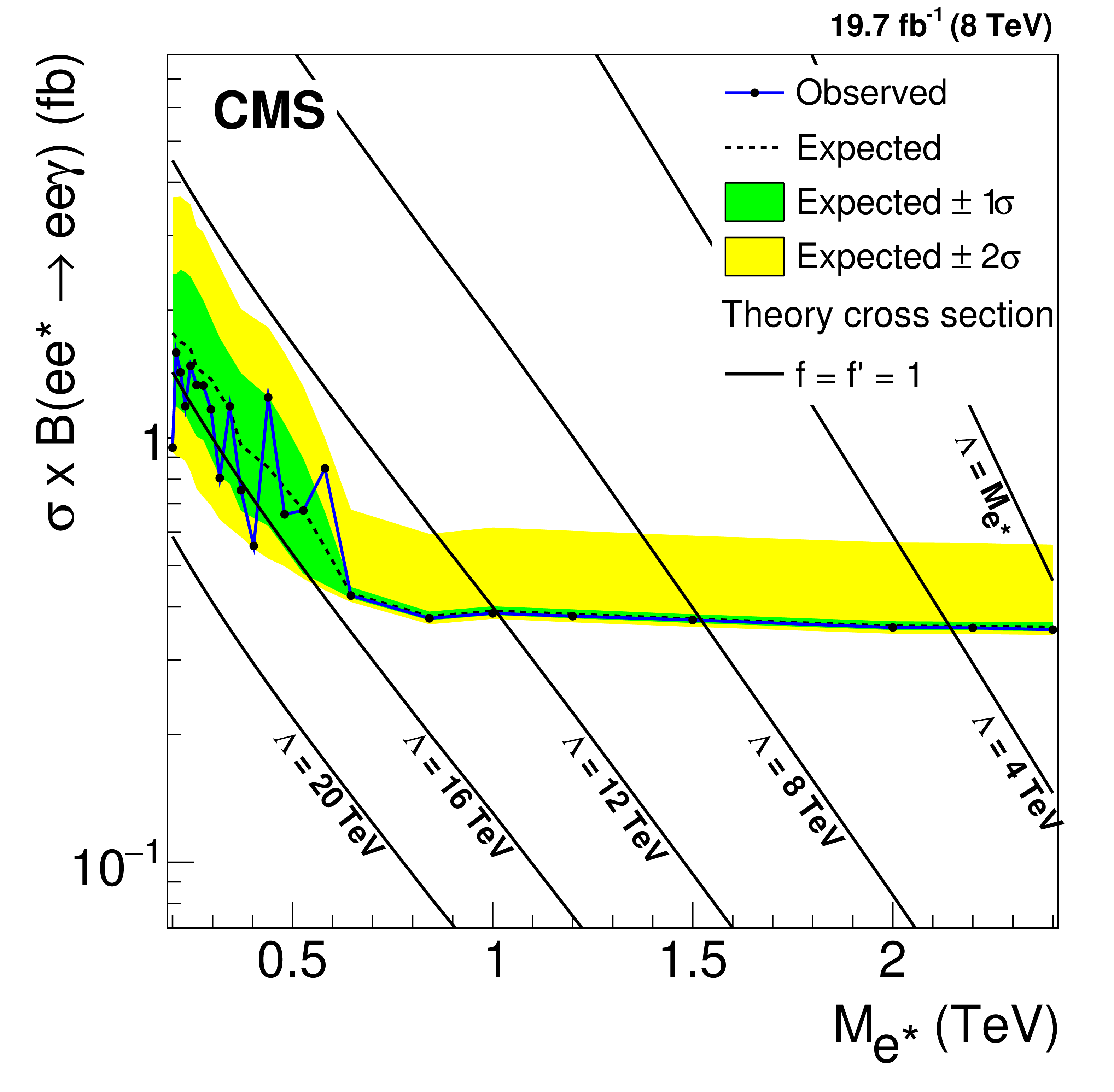
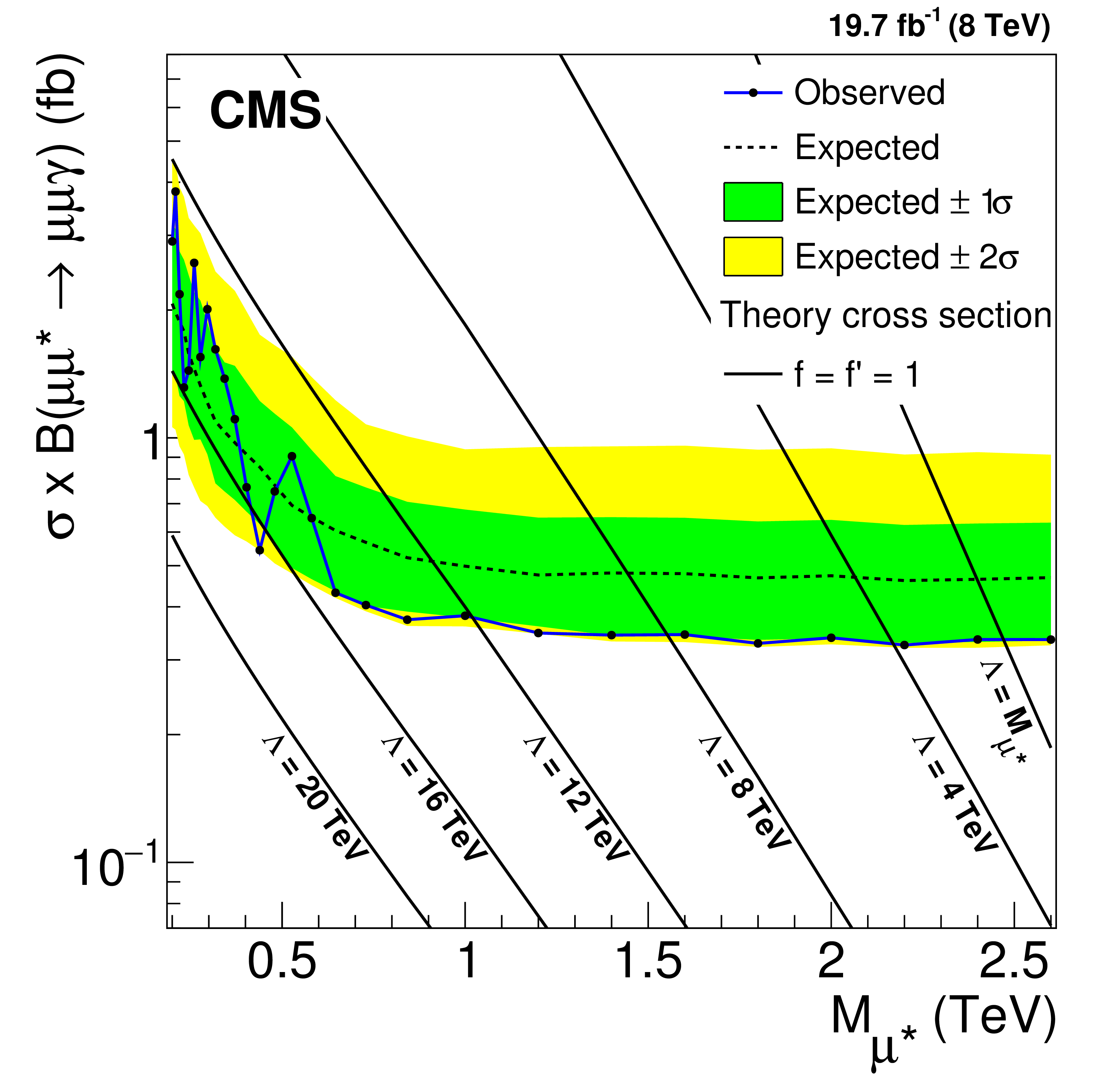
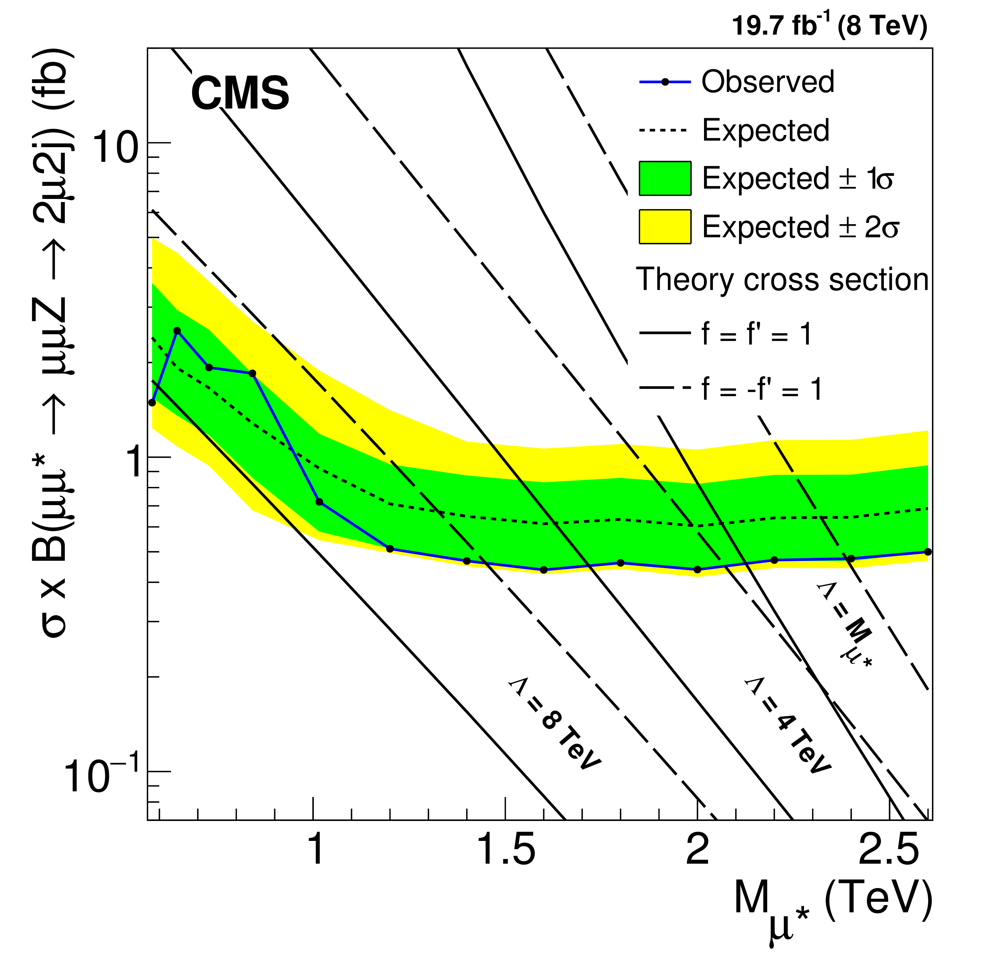
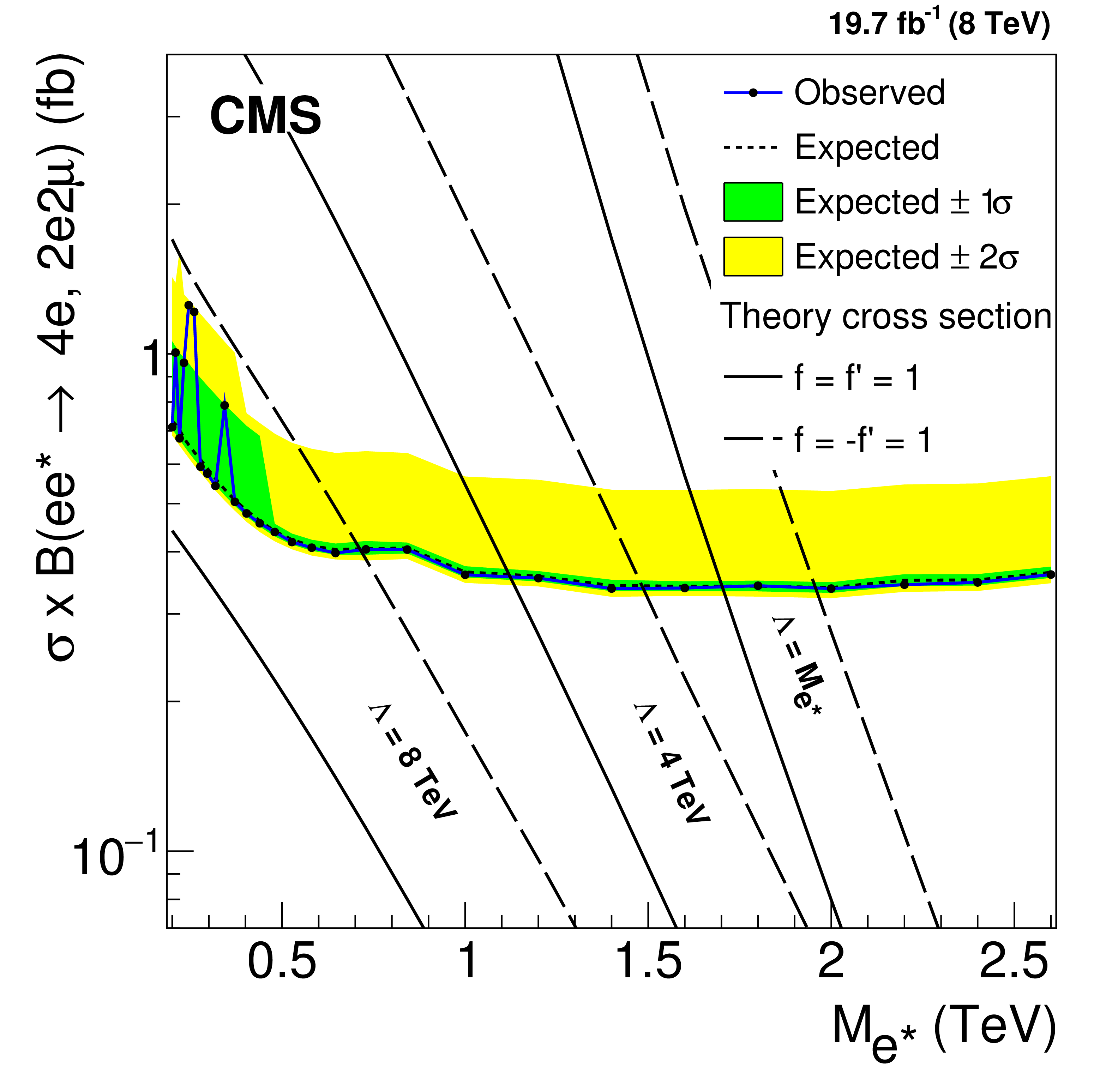
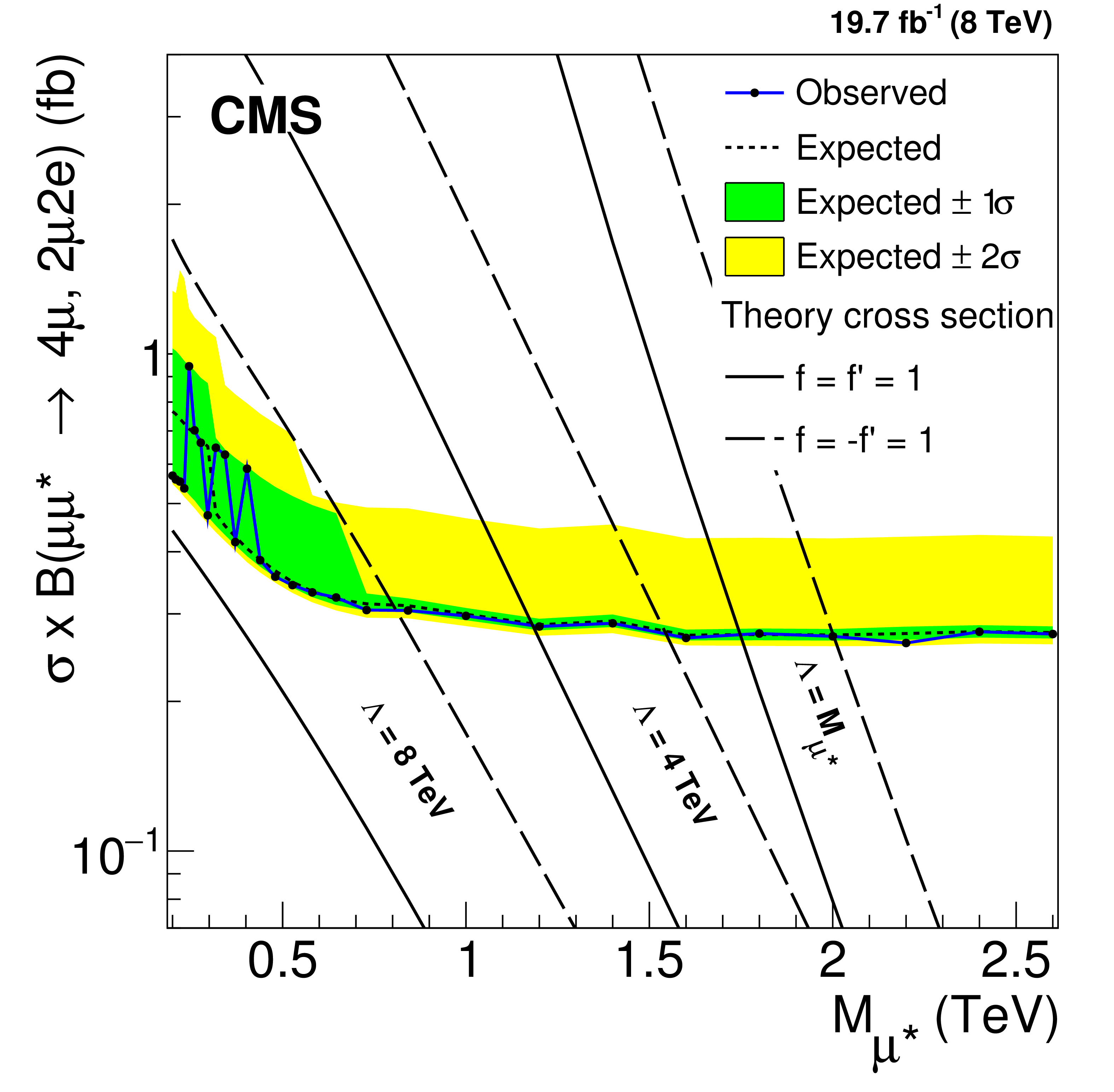
Figure 9-a:
Upper limits at 95% CL on the product of the production cross section and branching fraction for excited electrons (a,c,e) and excited muons (b,d,f). a,b: ${\ell \ell ^* \to \ell \ell \gamma } $, c,d: ${\ell \ell ^* \to \ell \ell \mathrm{ Z } \to 2\ell 2 {\mathrm {j}} } $, e,f: combined four-lepton results. It is assumed that the signal efficiency is independent of $\Lambda $. Theory curves are shown as solid or dashed lines. |
png pdf |
Figure 9-b:
Upper limits at 95% CL on the product of the production cross section and branching fraction for excited electrons (a,c,e) and excited muons (b,d,f). a,b: ${\ell \ell ^* \to \ell \ell \gamma } $, c,d: ${\ell \ell ^* \to \ell \ell \mathrm{ Z } \to 2\ell 2 {\mathrm {j}} } $, e,f: combined four-lepton results. It is assumed that the signal efficiency is independent of $\Lambda $. Theory curves are shown as solid or dashed lines. |

png pdf |
Figure 9-c:
Upper limits at 95% CL on the product of the production cross section and branching fraction for excited electrons (a,c,e) and excited muons (b,d,f). a,b: ${\ell \ell ^* \to \ell \ell \gamma } $, c,d: ${\ell \ell ^* \to \ell \ell \mathrm{ Z } \to 2\ell 2 {\mathrm {j}} } $, e,f: combined four-lepton results. It is assumed that the signal efficiency is independent of $\Lambda $. Theory curves are shown as solid or dashed lines. |
png pdf |
Figure 9-d:
Upper limits at 95% CL on the product of the production cross section and branching fraction for excited electrons (a,c,e) and excited muons (b,d,f). a,b: ${\ell \ell ^* \to \ell \ell \gamma } $, c,d: ${\ell \ell ^* \to \ell \ell \mathrm{ Z } \to 2\ell 2 {\mathrm {j}} } $, e,f: combined four-lepton results. It is assumed that the signal efficiency is independent of $\Lambda $. Theory curves are shown as solid or dashed lines. |
png pdf |
Figure 9-e:
Upper limits at 95% CL on the product of the production cross section and branching fraction for excited electrons (a,c,e) and excited muons (b,d,f). a,b: ${\ell \ell ^* \to \ell \ell \gamma } $, c,d: ${\ell \ell ^* \to \ell \ell \mathrm{ Z } \to 2\ell 2 {\mathrm {j}} } $, e,f: combined four-lepton results. It is assumed that the signal efficiency is independent of $\Lambda $. Theory curves are shown as solid or dashed lines. |
png pdf |
Figure 9-f:
Upper limits at 95% CL on the product of the production cross section and branching fraction for excited electrons (a,c,e) and excited muons (b,d,f). a,b: ${\ell \ell ^* \to \ell \ell \gamma } $, c,d: ${\ell \ell ^* \to \ell \ell \mathrm{ Z } \to 2\ell 2 {\mathrm {j}} } $, e,f: combined four-lepton results. It is assumed that the signal efficiency is independent of $\Lambda $. Theory curves are shown as solid or dashed lines. |
png pdf |
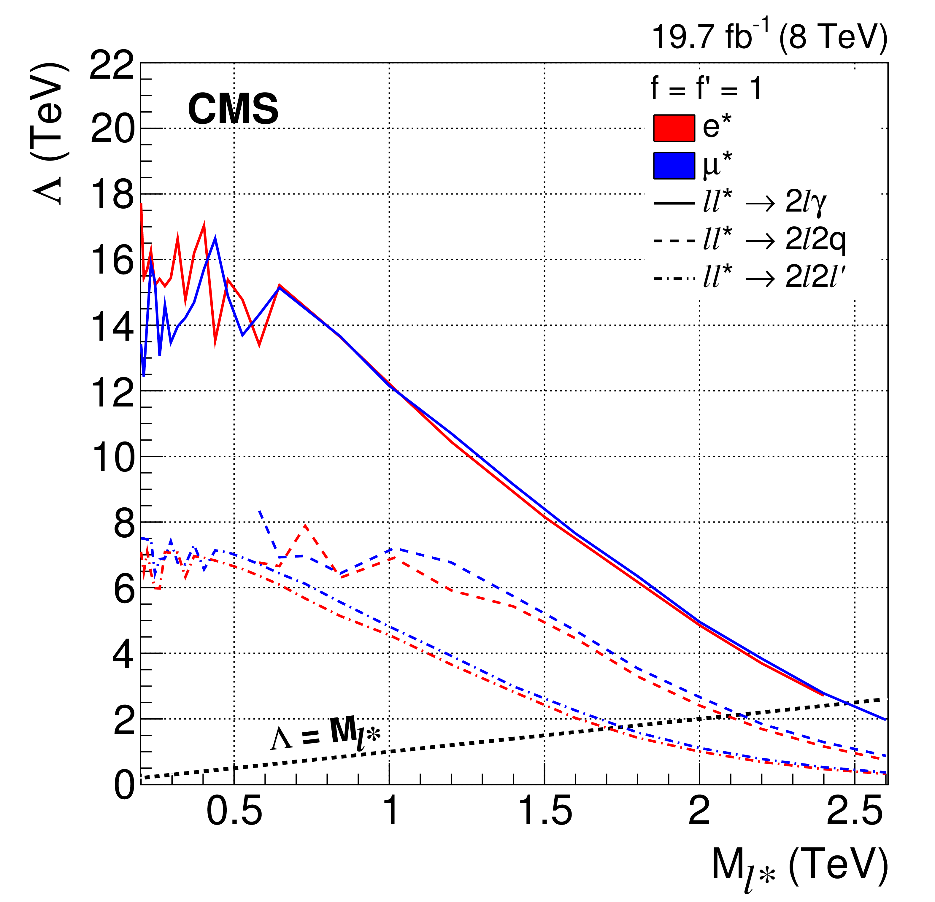
Figure 10-a:
Observed 95% CL limits on the compositeness scale $\Lambda $ for the cases $f = f^{\prime } =$ 1 and $f = -f^{\prime } =$ 1, as a function of the excited lepton mass for all channels. The excluded values are below the curves. |

png pdf |
Figure 10-b:
Observed 95% CL limits on the compositeness scale $\Lambda $ for the cases $f = f^{\prime } =$ 1 and $f = -f^{\prime } =$ 1, as a function of the excited lepton mass for all channels. The excluded values are below the curves. |
png pdf |
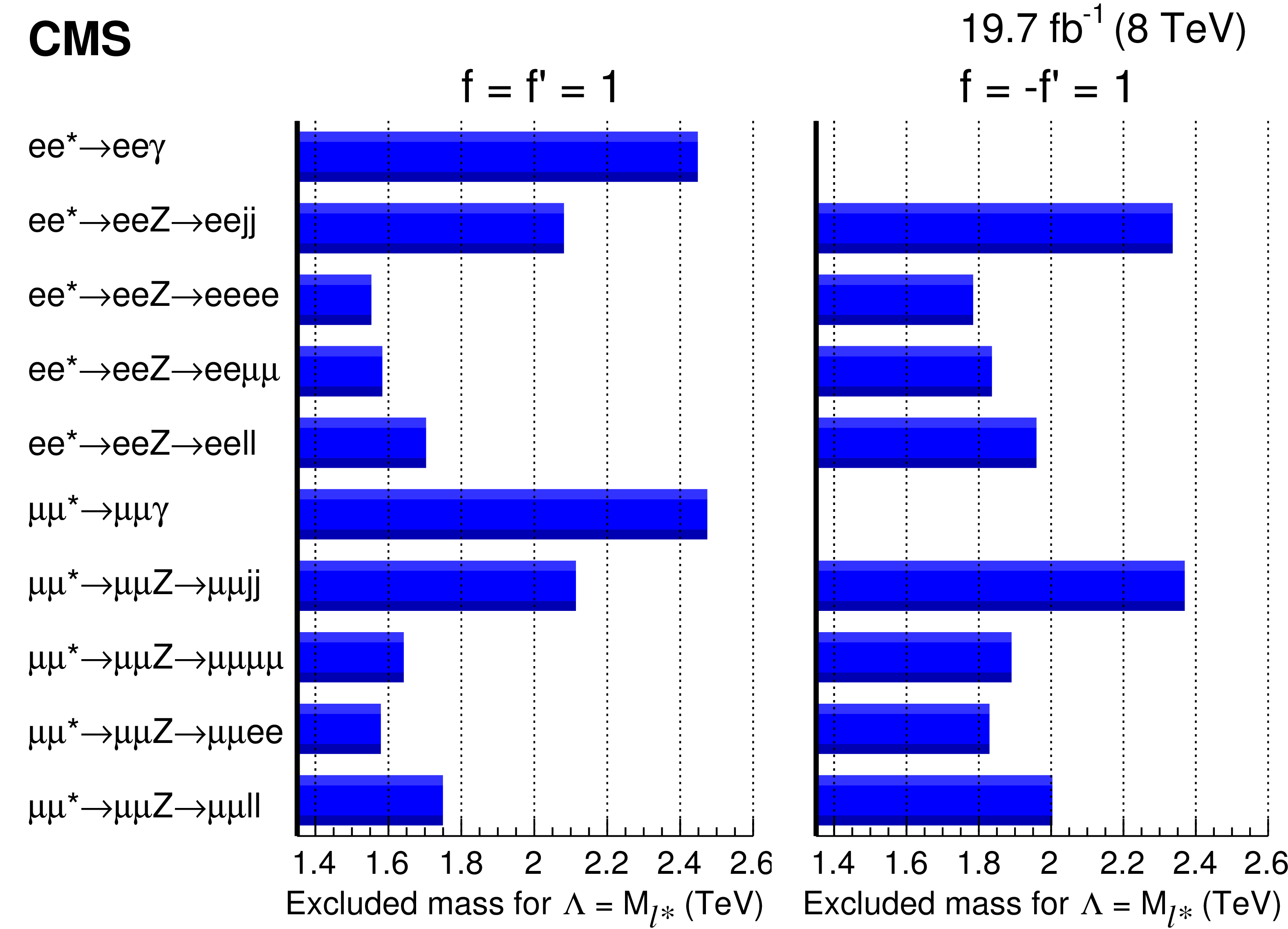
Figure 11:
Summary of all mass limits for the various channels and, including the combination of the four lepton channels, for $M_{\ell ^{*}} = \Lambda $. |
| Tables | |
png pdf |
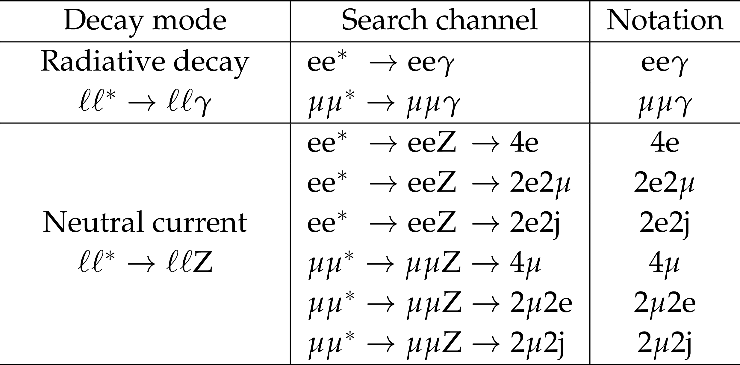
Table 1:
Final states for excited lepton searches considered in this analysis, where $\ell = \mathrm{ e } $, $\mu $. The notation for a specific channel is provided in the right most column. For neutral currents, the last two characters in this notation refer to particles from the decay of the Z boson. |

png pdf |
Table 2:
Excited lepton production cross section, and product of cross section and branching fraction for each of the three processes investigated, as a function of the mass of the excited lepton. The values of the k-factors are taken from Ref. [26]. The case $f = -f^{\prime } =$ 1 does not apply to the ${\ell \ell ^* \to \ell \ell \gamma }$ channel. |
png pdf |
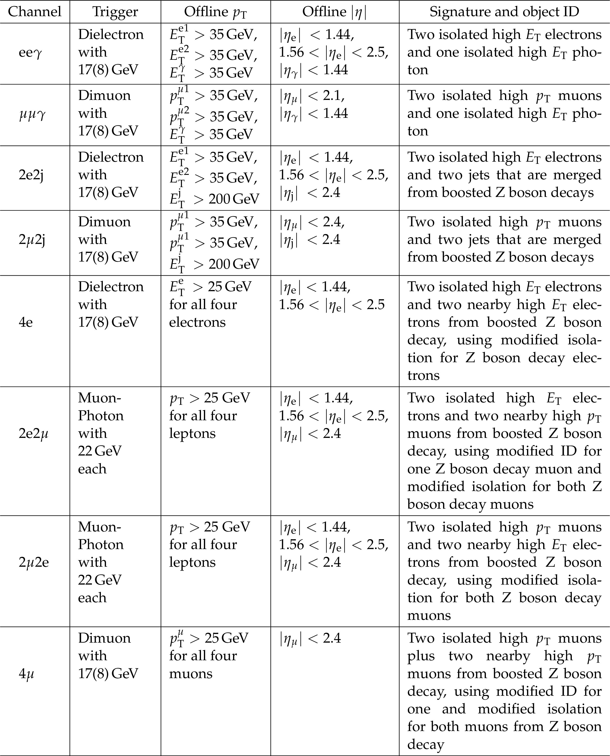
Table 3:
Trigger requirement, offline $ {p_{\mathrm {T}}} $ and $\eta $-selection criteria, and event signature for all final state channels of the ${\ell ^*}$ production and decay. |
png pdf |
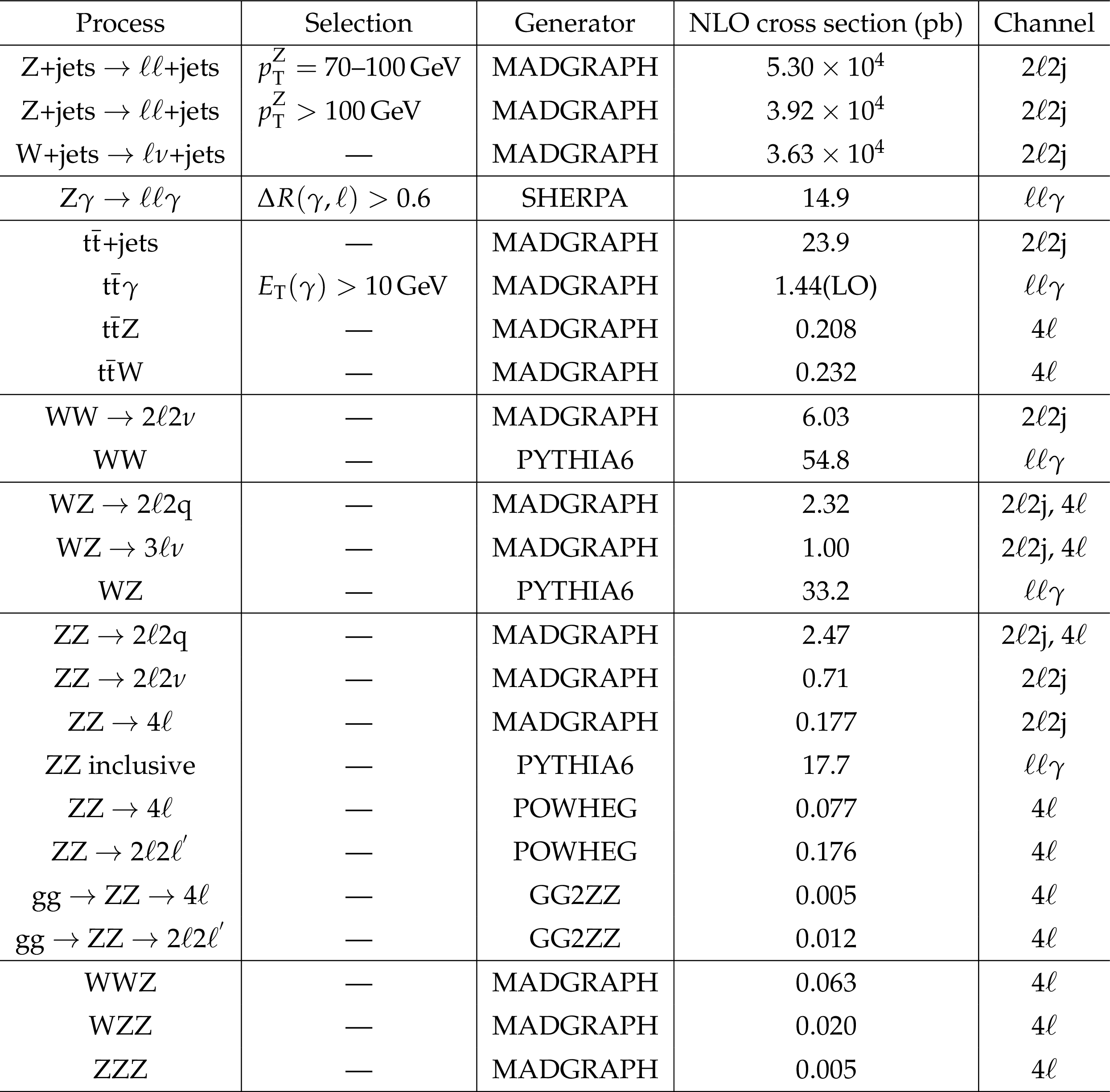
Table 4:
Background samples with the corresponding generator and cross sections used for the various channels. Specific generator selections are shown where important for the interpretation of the quoted cross sections. |
png pdf |
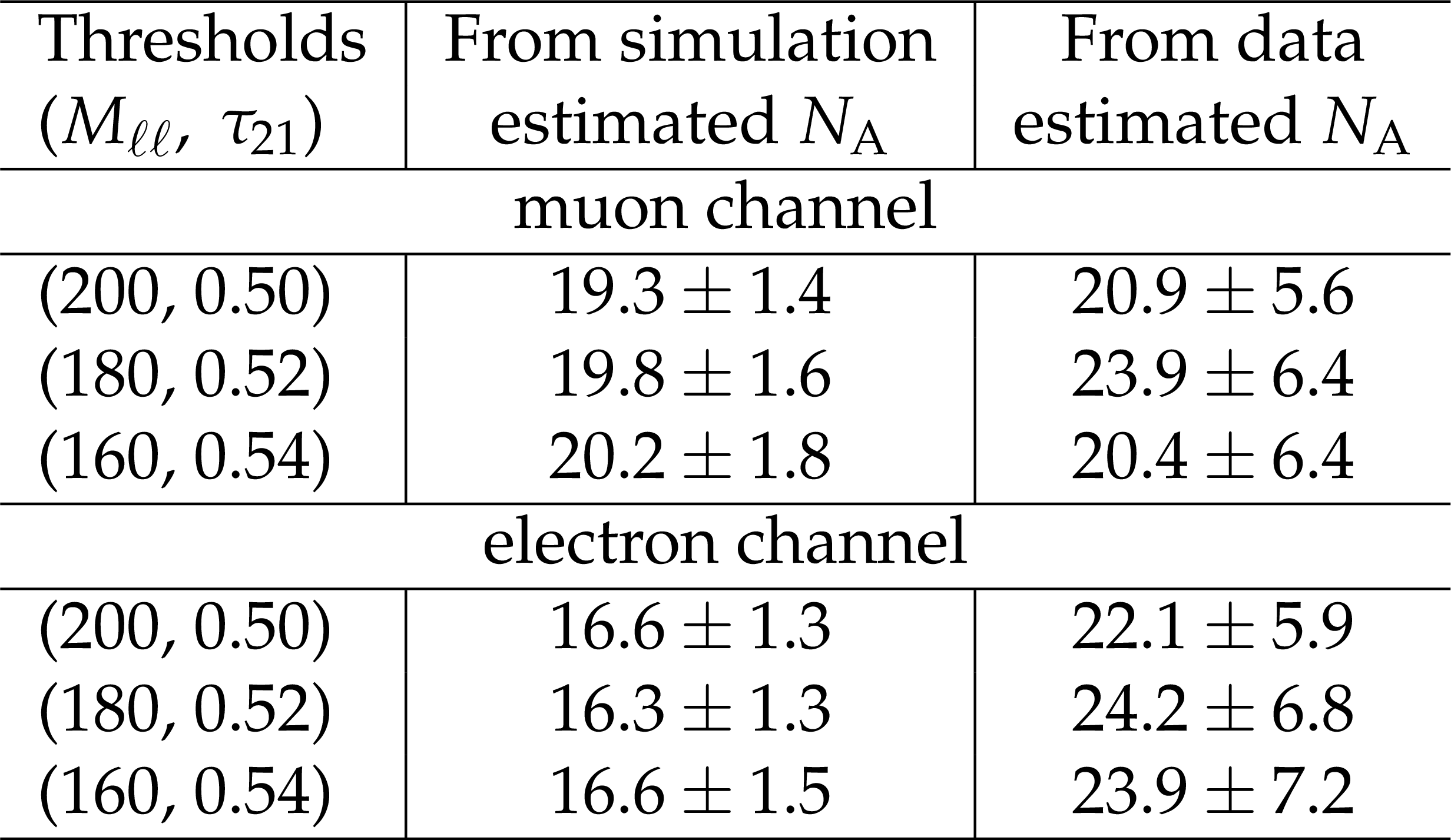
Table 5:
Events estimated in the region A by applying the ABCD method to simulated samples of DY+jets, $ {\mathrm{ t \bar{t} } } $+jets, and di-boson events, as well as to data: each time with a different set of defining boundaries for regions B, C and D. The true number of events in region A is 19.2 $\pm$ 1.3 and 15.0 $\pm$ 1.1 for the muon and electron channel, respectively. |
png pdf |
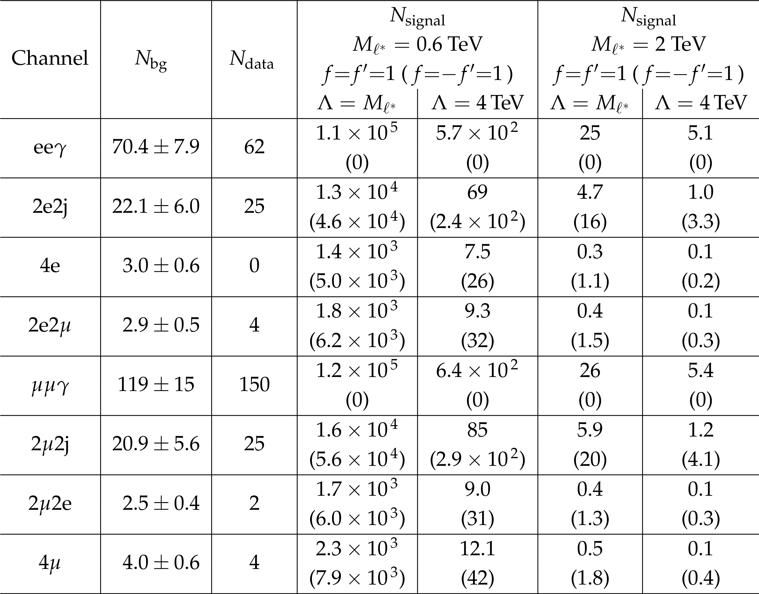
Table 6:
Expected background events, measured data events and expected signal yields for various channels before the L-shape optimization. Quoted uncertainties are the quadratic sum of statistical and systematic errors. The signal yields are presented for different values of $\Lambda $, for the cases $f = f^{\prime } =$ 1 and $f = -f^{\prime } =$ 1. No signal is expected in ${\ell \ell ^* \to \ell \ell \gamma }$ for $f = -f^{\prime } =$ 1. |
png pdf |
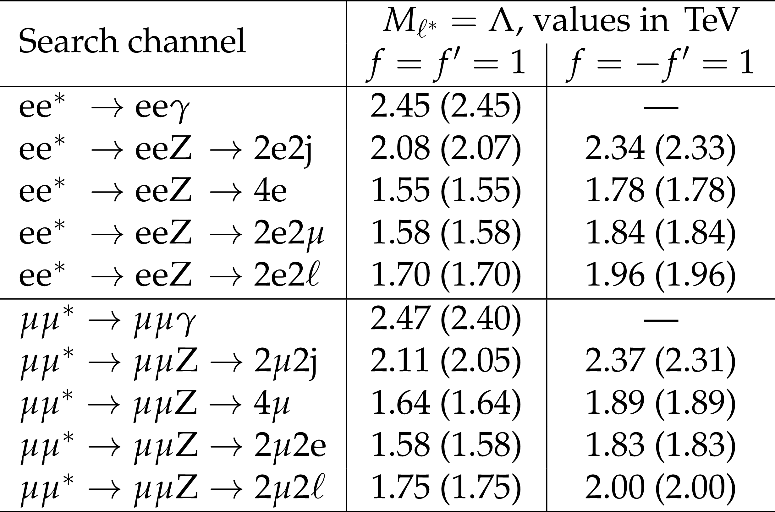
Table 7:
Summary of the observed (expected) limits on ${\ell ^*}$ mass, assuming ${M_{\ell ^*}} = \Lambda $, for the cases $f = f^{\prime } =$ 1 and $f = -f^{\prime } =$ 1. The latter case is not applicable to ${\ell \ell ^* \to \ell \ell \gamma } $. |
png pdf |
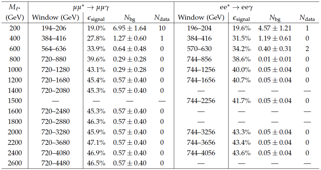
Table A1:
Final numbers used to calculate the cross section limits for the excited lepton channels resulting in photon emission, $\mu \mu ^* \rightarrow \mu \mu \gamma $ and $ \mathrm{e} \mathrm{e} ^* \rightarrow \mathrm{e} \mathrm{e} \gamma $ . |
png pdf |
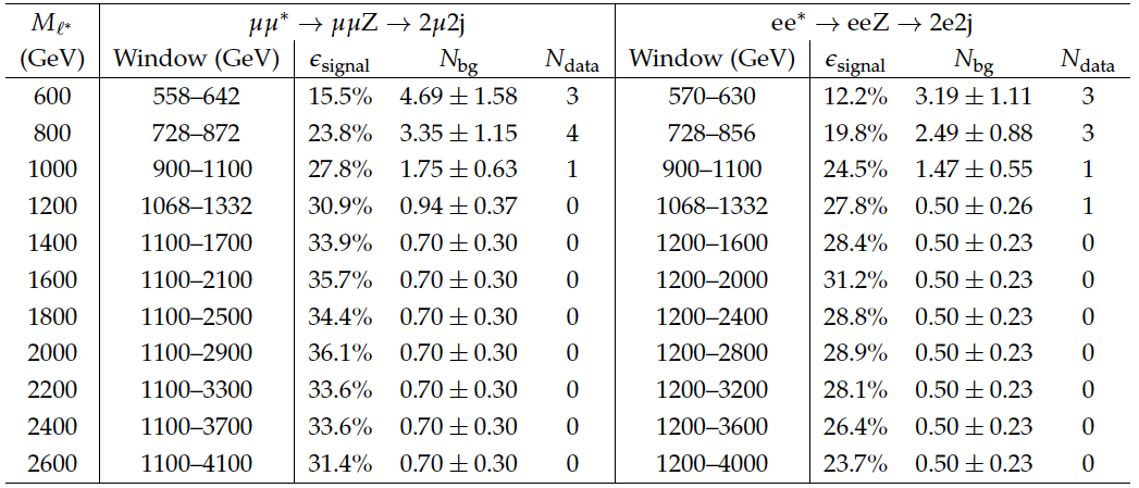
Table A2:
Final numbers used to calculate the cross section limits for the excited lepton channels resulting in the emission of a Z boson that decays to two jets, $\mu \mu ^* \rightarrow \mu \mu \mathrm{Z} \rightarrow 2\mu 2\mathrm{j}$ and $\mathrm{e} \mathrm{e} ^* \rightarrow \mathrm{e} \mathrm{e} \mathrm{Z} \rightarrow 2\mathrm{e} 2\mathrm{j}$ . |
png pdf |
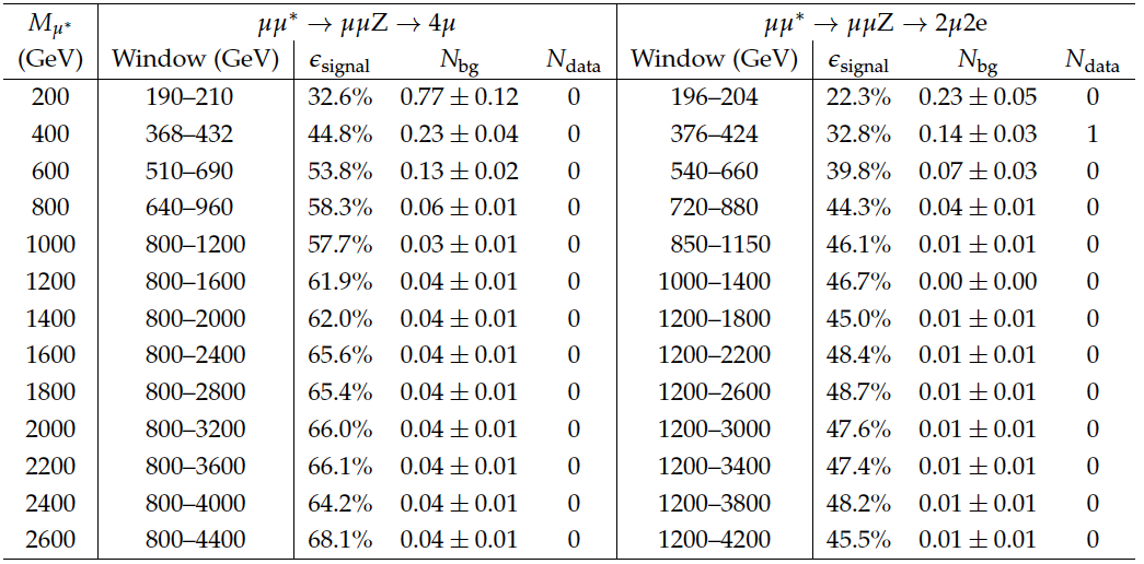
Table A3:
Final numbers used to calculate the cross section limits for the two excited muon channels in the 4$\ell $ final states. |

png pdf |
Table A4:
Final numbers used to calculate the cross section limits for the two excited electron channels in the 4$\ell $ final states. |
| Summary |
|
A comprehensive search for excited leptons, $ \mathrm{e} ^{*} $ and $ \mu ^{*} $, in various channels has been performed using 19.7 fb$^{-1}$ of pp collision data at $ \sqrt{s} = $ 8 TeV. The excited lepton is assumed to be produced via contact interactions in conjunction with the corresponding standard model lepton. Decaying to its ground state, the excited lepton may emit either a photon or a Z boson. No evidence of excited leptons is found and exclusion limits are set on the compositeness scale $\Lambda$ as a function of the excited lepton mass $ M_{\ell ^{*}} $. The $ \ell \ell \gamma $ final state has the largest production cross section and has therefore previously been used for searches. Following convention, the limits for the assumption $\Lambda = M_{\ell ^{*}} $ are included here. This final state yields the best limits, excluding excited electrons up to 2.45 TeV and excited muons up to 2.47 TeV, at 95% confidence level. These limits place the most stringent constraints to date on the existence of excited leptons. The $ \ell ^{*} \to \ell \mathrm{Z} $ decay channel has been examined for the first time at hadron colliders, allowing the case where couplings between standard model leptons and excited leptons $f = -f =$ 1 can be studied. The leptonic and hadronic (2-jet) final states of the Z boson are used in this search; these final states are Lorentz boosted, requiring a dedicated reconstruction strategy. The observed 95% exclusion limits extend to 2.34 (2.37) TeV for excited electrons (muons), for $f = -f^\prime =$ 1. |
|
|
Compact Muon Solenoid LHC, CERN |
|

|

|

|

|

|